Growth principles of natural hypergraphs
Abstract
Several systems can be represented by hypergraphs, an extension of graphs with associations between any number of vertices. These natural hypergraphs doe not appear at once. They are generated by some dynamical process of hypergraph evolution. Here I investigate what are the minimal growth principles of natural hypergraphs. I postulate edge duplication and vertex addition at edge duplications as the key principles of hypergraph growth. The implementation of these two principles induce the emergence of preferential attachment, power law degree distribution, the small-world property, high clustering coefficient and the founder effect. This work clarifies the distinction between principles, emergent properties and context specific details in the context of hypergraph growth dynamics.
I Introduction
In recent years there has been an increased interest in higher order associations beyond pairwise interactions Battiston et al. 2020; Battiston et al. 2021. Higher order associations have been represented by hypergraphs and simplicial complexes. Hypergraphs are combinatorial objects that generalizes graphs to include associations between more than two elements. Simplicial complexes are families of higher order associations that are closed under taking subsets (e.g., nodes, edges, triangles, …) and they are the building blocks of topological spaces. These mathematical constructions have been around for quite some time. The novelty is in how they appear in natural and human related systems Wang et al. 2010; Petri and Barrat 2018; Iacopini et al. 2019; Coutinho et al. 2020; Civilini et al. 2021; St-Onge et al. 2021; Neuhäuser et al. 2021, how they can be generated by random ensembles Chodrow et al. 2021; Young et al. 2021 and how they impact the behavior of process on such structures Vazquez 2009; Ghoshal et al. 2009; Courtney and Bianconi 2018.
When studying models of natural or human related systems we should make a distinction between principles, emergent properties and details. Let us take as an example preferential attachment in the context of networks Barabási and Albert 1999. There is no doubt preferential attachment is a distinctive feature in the dynamics of real networks. Yet, preferential attachment is an emergent property of local evolution rules on networks Vazquez 2003. When navigating a network the transversed links bias the walk to nodes with a higher number of neighbors (degree), with a bias proportional to the degree. New links generated by local walks on an existing network lead to preferential attachment Vazquez 2001. Making copies of existing nodes (e.g., web pages or proteins) generates preferential attachment as well Kleinberg et al. 1999; Pastor-Satorras et al. 2003; Vázquez et al. 2003; Chung et al. 2003. The local rules do more, they generate the small world property, high clustering coefficient and degree correlations Vazquez 2003.
In line with the timeline of growth models of networks, preferential attachment has been extended to the context hypergraph growth models Wang et al. 2010. Yet again, as in the context of networks, I would expect that preferential attachment is an emergent property of dynamical systems with a hypergraph structure. The basic mechanism should be rooted on some local dynamics.
Here I investigate the principles of natural hypergraphs growth dynamics. I have gotten inspiration from previous work on the topic Courtney and Bianconi 2018; Kovalenko et al. 2021. My contribution is to establish a clear separation between principles and consequence, cause and effect. I start in Section II postulating the principles of hypergraph evolution. I follow in Section III with an analysis of hypergraph properties derived from those principles. The emphasis is on the emergent properties: preferential attachment Barabási and Albert 1999, scale-free degree distribution Albert et al. 1999, small-world and high clustering coefficient Watts and Strogatz 1998. In Section III.3 I elaborate on the founder effect as another emergent property. Finishing with concluding remarks in Section IV.
II Principles
Preferential attachment and scale-free degree distributions are consequencse of network dynamics with local evolution rules Vazquez 2003. In a nutshell, whenever we transverse an edge we are performing a bias sampling towards vertices with higher degrees. Selecting an edge, rather than a vertex, is what drives the preferential attachment to vertices with higher degree. Since many of the networks studied in the past are actually projections of latent hypergraphs (e.g., co-autorships and metabolic networks), I expect that similar principles apply to the dynamics of natural and human related hypergraphs.
A hypergraph is composed by a set of vertices and a set of edges , where edges are sets with one or more vertices. When there are not two edges with the same vertex composition we call it a simple hypergraph, or a multi-hypergraph otherwise. Following the principles of network evolution, I focus on local and edge centric evolution principles of hypegraphs. Local means that the evolution rules are based on one or a few edges in a local neighborhood of the hypergraph. The simplest local rule of hypergraph growth is edge duplication
| (1) |
There are several natural and human related scenarios that are represented in this rule. Starting with the obvious resemblance with asexual reproduction by cell division. If vertices are genes and edges are cells then Eq. (1) is a model of cell division. In the context of human behavior an edge can be an instance of a recurrent activity involving a group of people (the vertices). Examples include scientific publications, scientific meetings and working days at institutions departments. Notice that Eq. (1) generates multi-hypergraphs or temporal hypergraphs if we add a time stamp label to each edge.
We need a second rule to model the addition of new vertices. The simplest of local edge centric rules is duplication with vertex addition at the duplicate
| (2) |
In asexual reproduction this rule represents gene duplication, an event that can happen during the genome replication preceding cell division. In the context of human behavior Eq. (2) represents a new individual joining a group at their next group meeting. We could spell further evolution rules involving two or more edges that are adjacent (thus local) leading to edge composition mixing. Here I will stop at the two simplest rules (1)-(2) and investigate the structure of hypergraphs they generate.
III Emergent properties
To investigate the emergent properties from the hypergraph growth principles I introduce a specific model. At time we start with hypergraph . At each subsequent time step, we select an edge sampled with equal probability among all current edges. To this edge we apply (1) with probability or (2) otherwise. When (1) is applied, we create a new edge with the exact same vertex composition. When (2) is applied, we add a new vertex and a new edge with the composition of plus the new vertex. We continue until the hypergraph has vertices. Since new vertices are added with probability , represents the vertex growth rate per edge duplication. Each hypergraph ensemble is parametrized by .
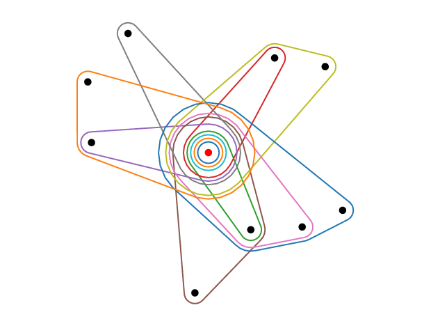
A Python implementation is listed in Appendix A. A hypergraph example generated with this code is shown in Fig. 1. The star-like shape already anticipates the heterogeneity in the vertices connectivity and the small world property.
III.1 Preferential attachment
The degree of a vertex is the number of edges containing that vertex and it will be denoted by . At each step one edge is selected for duplication, with or without vertex addition. The probability that a vertex with degree is in the selected edge, and therefore increases its degree, is
| (3) |
where is the number of edges at step . That is preferential attachment: new edges are added at vertices with a bias by their degree.


III.2 Power law degree distribution
For large hypergraphs (), the rate equation describing the evolution of the number of vertices with degree is
| (4) | |||||
Since an edge is added at each step and vertices are added at rate , and for . In such a case Eq. (4) has the steady state solution , where satisfies the recursive equation
| (5) |
Iterating this equation with the boundary condition I obtain
| (6) |
The degree distribution of hypergraphs generated by (1)-(2) have a power low tail with exponent -2. This is corroborated by numerical simulations (Fig. 2).
In many applications the hypergraph is projected into a graph, where two vertices are connected if there is at least one edge containing them (on-vertex projection). The vertex degree in this graph is the number of nearest neighbors, the number of other vertices that can be reached via the edges containing the vertex. Although I do not have an analytical derivation for the number of neighbors distribution, I expect it is characterized by the same power law tail with exponent -2. This seems to be the cased based on numerical simulations (Fig. 3)


III.3 Founder effect
Visual inspection of Fig. 1 indicates that the seeding vertex is part of all edges. This is indeed the case. If we start with one edge containing one or more vertices then all other edges will contain those starting vertices. The founders persist in all edges.
This behavior can be relaxed if we specify further rules. For example, during the growth of organizations large departments are split and new managers are brought in to maintain communication between the new departments. This can be modeled by duplication with edge split and vertex addition
| (7) |
where . A specific implementation with random and balance edge split is found in Appendix B. Figure 4 shows an example with edges constrained to size 2. The vertex in the far right does not share an edge with the founder (in red). Yet, the founder is still connected to most vertices.
A founder is basically a member that joined the system early in its evolution and it has a high connectivity at later times. This is illustrated in Fig. 5, with the founder highlighted in red. In fact, that plot is an operational method to identify putative founders. They are found in the upper left corner.

III.4 Small-world property
The founder effect induces the small-world property. The hypergraphs generated by (1)-(2) have diameter 2. Any two vertices are at most two edges away, each edge containing the founder. This singular behavior of constant diameter is relaxed after adding the edge split rule (7). When a cap is imposed in the edge size there is a logarithmic increase in the average shortest path distance with increasing the number of vertices (Fig. 6), the typical behavior of small-world networks Amaral et al. 2000. Furthermore, the larger the maximum allowed edge size the smaller the hypergraph, getting closer to the unconstrained case (Fig. 6, blue symbols).
III.5 High clustering coefficient
The hypergraph extension to include edges with size larger than 2 induces a high clustering coefficient in the associated graph on-vertex projection. Not surprisingly hypergraphs evolving through the growth principles introduced here have a high clustering coefficient. The numerical estimates of the average clustering coefficient are above 0.5 for the range of parameters investigated (see Table 1).
| H1 | 2 | 0.1 | 2.25 | 0.55 | -0.53 |
| H1 | 2 | 0.5 | 4.54 | 0.76 | -0.07 |
| H1 | 2 | 0.9 | 4.69 | 0.74 | -0.07 |
| H1 | 0 | 0.1 | 2.00 | 0.55 | -0.59 |
| H1 | 0 | 0.5 | 1.99 | 0.91 | -0.22 |
| H1 | 0 | 0.9 | 1.99 | 0.92 | -0.15 |
| H10 | 2 | 0.1 | 2.14 | 0.93 | 0.07 |
| H10 | 2 | 0.5 | 3.31 | 0.80 | 0.05 |
| H10 | 2 | 0.9 | 4.25 | 0.75 | 0.18 |
| H10 | 0 | 0.1 | 1.98 | 0.98 | -0.01 |
| H10 | 0 | 0.5 | 1.97 | 0.97 | -0.03 |
| H10 | 0 | 0.9 | 1.97 | 0.95 | -0.03 |
III.6 Degree correlations
Degree correlations inform about degree mixing between connected vertices Pastor-Satorras et al. 2001; Newman 2002. Degree correlations are quantified by the Pearson correlation of the degree of connected vertices, denoted by Newman 2002. When we say there is assortative mixing, whereby connected vertices tend to have similar degrees. When we say there is disassortative mixing, whereby connected vertices tend to have dissimilar degrees. For hypergraphs we can use the same quantity, interpreting connected vertices as vertices sharing at least one hyper-edge.
The hypergraphs generated by (1)-(2) or (1)+(7) have variable values of ranging from negative to positive values (Tab. 1). is modulated by the founder effect. For example, when the starting hypergraph has one edge containing one vertex then for all values of and the maximum edge size that I have simulated. In contrast, when the starting hypergraph has one edge containing 10 vertices then for but for , for all simulated values of . Therefore degree correlations are sensitive to parameters and initial conditions. They are context depending.
IV Conclusions
Edge duplication and vertex addition at edge duplication are natural principles of hypergraph evolution. The universal properties of real world networks that are projections of hypergraphs are emergent properties from these two growth principles.
The evolution of natural or human related hypergraphs is richer. I have illustrated the impact of adding a constraint on the maximum edge size. Higher order evolution rules can involve two or more edges. These variations will modulate the emergent properties described above. They could modify the exponent of the power law tail in the degree distribution or increase the diameter. Yet, as long as the hypergraph growth principles of edge duplication and vertex addition at edge duplication are part of the system dynamics the emergent properties will persist.
The founder effect modulates the hypergraph properties. The founder effect is a typical property of natural systems that grow from a small initial seed. Biological populations of organisms is the canonical example. The founder effect is observed during the creation of new academic fields or institutions. Based on this work, the founder effect is an emergent property of the hypergraph growth principles.
Acknowledgements
Nodes & Links did not have any role in the study design, data collection and analysis, decision to publish, or preparation of the manuscript.
Appendix A
Implementation of (1)-(2) in Python
import numpy as np
import hypernetx as hnx
def HGP(n, mu, E0, seed):
    # hypergraph by growth principles
    np.random.seed(seed)
    E = E0
    i = max([j for e in E for j in e]) + 1
    while i<n:
        e = E[np.random.randint(len(E))]
        if np.random.random() < mu:
            E.append(e + [i])
            i += 1
        else:
            E.append(e)
    return E
E = HP1(10, 0.5, [[0]], 100)
H = hnx.Hypergraph(E)
hnx.drawing.draw(H)
Appendix B
Implementation of (1)+(7) inPpython
import numpy as np
import hypernetx as hnx
def HGPSC(n, mu, E0, seed, sc):
    # hypergraph growth principles
    #   with edge size constraint
    np.random.seed(seed)
    E = E0
    i = max([j for e in E for j in e]) + 1
    while i<n:
        e = E[np.random.randint(len(E))]
        if np.random.random() < mu:
            if len(e)<sc:
                E.append(e + [i])
            else:
                split = np.array_split(
                    np.random.permutation(e),2)
                E.append(list(split[0])+[i])
                E.append(list(split[1])+[i])
            i += 1
        else:
            E.append(e)
    return E
E = HGPSC(10, 0.5, [[0]], 100, 2)
H = hnx.Hypergraph(E)
hnx.drawing.draw(H)
References
- Battiston et al. (2020) F. Battiston, G. Cencetti, I. Iacopini, V. Latora, M. Lucas, A. Patania, J.-G. Young, and G. Petri, Physics Reports 874, 1 (2020).
- Battiston et al. (2021) F. Battiston, E. Amico, A. Barrat, G. Bianconi, G. Ferraz de Arruda, B. Franceschiello, I. Iacopini, S. Kéfi, V. Latora, Y. Moreno, M. M. Murray, T. P. Peixoto, F. Vaccarino, and G. Petri, Nature Physics 17, 1093 (2021).
- Wang et al. (2010) J.-W. Wang, L.-L. Rong, Q.-H. Deng, and J.-Y. Zhang, Eur. Phys. J. B 77, 493 (2010).
- Petri and Barrat (2018) G. Petri and A. Barrat, Phys. Rev. Lett. 121, 228301 (2018).
- Iacopini et al. (2019) I. Iacopini, G. Petri, A. Barrat, and V. Latora, Nature Comm. 10, 2485 (2019).
- Coutinho et al. (2020) B. C. Coutinho, A.-K. Wu, H.-J. Zhou, and Y.-Y. Liu, Phys. Rev. Lett. 124, 248301 (2020).
- Civilini et al. (2021) A. Civilini, N. Anbarci, and V. Latora, Phys. Rev. Lett. 127, 268301 (2021).
- St-Onge et al. (2021) G. St-Onge, H. Sun, A. Allard, L. Hébert-Dufresne, and G. Bianconi, Phys. Rev. Lett. 127, 158301 (2021).
- Neuhäuser et al. (2021) L. Neuhäuser, R. Lambiotte, and M. T. Schaub, Phys. Rev. E 104, 064305 (2021).
- Chodrow et al. (2021) P. S. Chodrow, N. Veldt, and A. R. Benson, Science Adv. 7, eabh1303 (2021).
- Young et al. (2021) J.-G. Young, G. Petri, and T. P. Peixoto, Comm. Phys. 4, 1 (2021).
- Vazquez (2009) A. Vazquez, J. Stat. Mech.: Theory Exp. 2009, P07006 (2009).
- Ghoshal et al. (2009) G. Ghoshal, V. Zlatić, G. Caldarelli, and M. E. J. Newman, Phys. Rev. E 79, 066118 (2009).
- Courtney and Bianconi (2018) O. T. Courtney and G. Bianconi, Phys. Rev. E 97, 052303 (2018).
- Barabási and Albert (1999) A.-L. Barabási and R. Albert, Science 286, 509 (1999).
- Vazquez (2003) A. Vazquez, Phys. Rev. E 67, 056104 (2003).
- Vazquez (2001) A. Vazquez, Europh. Lett. 54, 430 (2001).
- Kleinberg et al. (1999) J. M. Kleinberg, R. Kumar, P. Raghavan, S. Rajagopalan, and A. S. Tomkins, in Computing and Combinatorics, Lecture Notes in Computer Science, edited by T. Asano, H. Imai, D. T. Lee, S.-i. Nakano, and T. Tokuyama (Springer, Berlin, Heidelberg, 1999) pp. 1–17.
- Pastor-Satorras et al. (2003) R. Pastor-Satorras, E. Smith, and R. V. Solé, J. Theor. Biol. 222, 199 (2003).
- Vázquez et al. (2003) A. Vázquez, A. Flammini, A. Maritan, and A. Vespignani, Complexus 1, 38 (2003).
- Chung et al. (2003) F. Chung, L. Lu, T. G. Dewey, and D. J. Galas, J. Comp. Biol. 10, 677 (2003).
- Kovalenko et al. (2021) K. Kovalenko, I. Sendiña-Nadal, N. Khalil, A. Dainiak, D. Musatov, A. M. Raigorodskii, K. Alfaro-Bittner, B. Barzel, and S. Boccaletti, Comm. Phys. 4, 1 (2021).
- Albert et al. (1999) R. Albert, H. Jeong, and A.-L. Barabási, Nature 401, 130 (1999).
- Watts and Strogatz (1998) D. J. Watts and S. H. Strogatz, Nature 393, 440 (1998).
- Amaral et al. (2000) L. A. N. Amaral, A. Scala, M. Barthélémy, and H. E. Stanley, Proceedings of the National Academy of Sciences 97, 11149 (2000).
- Pastor-Satorras et al. (2001) R. Pastor-Satorras, A. Vázquez, and A. Vespignani, Phys. Rev. Lett. 87, 258701 (2001).
- Newman (2002) M. E. J. Newman, Phys. Rev. Lett. 89, 208701 (2002).