Enhancing the Robustness via Adversarial Learning and Joint Spatial-Temporal Embeddings in Traffic Forecasting
Conference: Proceedings of the 32nd
ACM International Conference on Information and Knowledge
Management; October 21–25, 2023; Birmingham, United KingdomProceedings of the 32nd ACM International Conference on
Information and Knowledge Management (CIKM ’23), October 21–25, 2023,
Birmingham, United KingdomPrice: 15.00DOI: 10.1145/3583780.3614868ISBN: 979-8-4007-0124-5/23/10CCS: Information systems Spatial-temporal systemsCCS: Networks Network robustness
Abstract.
Traffic forecasting is an essential problem in urban planning and computing. The complex dynamic spatial-temporal dependencies among traffic objects (e.g., sensors and road segments) have been calling for highly flexible models; unfortunately, sophisticated models may suffer from poor robustness especially in capturing the trend of the time series (1st-order derivatives with time), leading to unrealistic forecasts. To address the challenge of balancing dynamics and robustness, we propose TrendGCN, a new scheme that extends the flexibility of GCNs and the distribution-preserving capacity of generative and adversarial loss for handling sequential data with inherent statistical correlations. On the one hand, our model simultaneously incorporates spatial (node-wise) embeddings and temporal (time-wise) embeddings to account for heterogeneous space-and-time convolutions; on the other hand, it uses GAN structure to systematically evaluate statistical consistencies between the real and the predicted time series in terms of both the temporal trending and the complex spatial-temporal dependencies. Compared with traditional approaches that handle step-wise predictive errors independently, our approach can produce more realistic and robust forecasts. Experiments on six benchmark traffic forecasting datasets and theoretical analysis both demonstrate the superiority and the state-of-the-art performance of TrendGCN. Source code is available at https://github.com/juyongjiang/TrendGCN.
Keywords:
Spatial-Temporal Embeddings; Robustness; Traffic Forecasting1. Introduction
Traffic forecasting, as one of the essential parts of the intelligent transportation system, plays an irreplaceable role in developing a smart city (Jiang and Luo 2021; Jiang et al. 2021). It aims to accurately predict future traffic data, e.g., traffic flow and speed, given historical traffic data recorded by sensors on a road network (Li et al. 2018). It is a highly challenging task due to dynamic spatial and temporal dependencies within the road network. As shown in Fig. 1, spatially, the traffic conditions of nearby sensors have dynamic dependencies on each other. Temporally, current traffic data are dependent on historical observations in a dynamic way. Spatial and temporal dependencies vary with time due to various factors, e.g., weather and traffic accidents.

Many approaches have been proposed for traffic forecasting, continuously improving from shallow machine learning (Williams and Hoel 2003; Zivot and Wang 2006; Wu et al. 2004) to recurrent neural network (RNN) and convolutional neural network (CNN) based deep learning (SHI et al. 2015; Ma et al. 2017; Yu et al. 2017). Although these works can capture temporal dependencies and regular spatial dependencies, they can not adequately model non-Euclidean spatial dependencies dominated by irregular road networks. Towards this problem, graph neural networks (GNN) (Thomas N. Kipf 2017) have been introduced in traffic forecasting owing to their superior ability to deal with irregular graph-structured data. These GNN-based works normally represent sensors as nodes and spatial dependencies between sensors as edges and leverage adjacency matrices to describe spatial dependencies of road networks (Wu et al. 2021; Jiang and Luo 2021). Recently, spatial-temporal graph neural networks (STGNNs) (Li et al. 2018; Yu et al. 2018; Guo et al. 2019; Zheng et al. 2020; Guo et al. 2021; Lan et al. 2022), a group of approaches integrating GNNs to model spatial dependencies with RNNs, CNNs, or Attentions to model temporal dependencies, have shown the state-of-the-art performance for traffic forecasting.
Despite the success, there are still some limitations with current STGNNs, which we discuss below.
Firstly, most existing STGNNs rely on a basic assumption that spatial dependencies are fixed over time. Therefore, static graphs, e.g., distance graphs (Yu et al. 2018; Guo et al. 2019; Guo et al. 2021), temporal similarity graphs (Li and Zhu 2021a; Fang et al. 2021), static adaptive graphs (Bai et al. 2020; Wu et al. 2020a), and their combinations (Wu et al. 2019; Geng et al. 2019; Khaled et al. 2022), are typically used to model spatial dependencies. These works do not cater to the changing nature of dependencies between nodes (shown in Fig. 1(a)) and cannot handle dynamic spatial dependencies. Some attempts (Zhang et al. 2020; Li et al. 2023; Lan et al. 2022) have tried to model such dynamics for traffic forecasting. They design feature extraction mechanisms to quantify changing patterns from the data, and with the help of domain knowledge (e.g., road occupancy rates and weather conditions) to construct time-varying spatial graphs. Compared to those based on static graphs, these works can make more realistic predictions. However, when there exist outlier points or interrupts, they could generate bad predictions, due to the sensitivity to the temporal changes (see Fig. 2(b)). Such a phenomenon calls for effective constraints on global properties for robust time series forecasting.
Intuitively, since the trend of traffic data represents the average traffic conditions over time, we take the trend as a representative global property of time series. However, most existing STGNNs (Wu et al. 2021; Jiang and Luo 2021; Jiang et al. 2021) adopt the mean absolute error (MAE) as a loss function to evaluate the predictions and supervise the model training, which treats each predicted result individually and can not take the trends for global constraints. As illustrated in Fig. 2(a), the blue and the pink curves have the same magnitude . The blue curve looks less desirable than the pink one when a sudden change happens around , as its trend is opposite to that of the ground truth, while the pink curve is consistent with the ground truth. Therefore, we should introduce more reliable constraints on trends. In particular, we term the phenomenon that predictions have different trends with the same loss values as trend discrepancy.
Recently, a few works (Wu et al. 2020b; Khaled et al. 2022) have been proposed to eliminate trend discrepancies via GAN. They construct the true and fake samples for discriminators by concatenating inputs with predictions (from the generator) and ground truth (from the dataset), respectively. Since these works take the whole sequence in error evaluation, they can eliminate trend discrepancies and error accumulation to some extent. However, the dynamic spatial dependencies in the generator are not fully taken into account, which are crucial to capturing the changing nature of traffic systems. Moreover, spatial dependencies in the predicted results are not modelled explicitly. Since spatial dependencies reflect the hidden correlations between the trends of traffic data, they should also align with the dependencies in the ground truth.

To this end, we propose TrendGCN to solve the two aforementioned problems: 1) how to model dynamic spatial dependencies concisely and effectively; 2) how to coordinate the trend discrepancies with dynamic modeling to improve the robustness. The main contributions of our work are summarized as follows:
- •
We propose TrendGCN, a new scheme combing the flexibility of GCNs and the capacity of generative and adversarial loss in sequential data with inherent statistical correlations. It employs simultaneous spatial (node-wise) embedding and temporal (time-wise) embedding to account for heterogeneous space-and-time convolutions.
- •
We introduce adversarial training to systematically evaluate both the trend-level and dependency-level discrepancies between the true data and the predicted results, thus being more robust in generating a desired trend than handling step-wise prediction errors independently.
- •
We evaluate the proposed model on six benchmarks traffic forecasting datasets. Extensive experiments and theoretical analysis both demonstrate the superiority and the state-of-the-art performance of TrendGCN.
2. Related Work
2.1. STGNNs for Traffic Forecasting
Spatial-temporal graph neural networks (STGNNs) (Li et al. 2018; Yu et al. 2018; Geng et al. 2019; Guo et al. 2019; Zheng et al. 2020; Guo et al. 2021) have shown remarkable performance and achieved state-of-the-art in traffic forecasting. They mainly integrate GNNs to model non-Euclidean spatial dependencies with RNNs, CNNs, and Attentions to model temporal dependencies (Wu et al. 2021; Jiang and Luo 2021). However, many existing STGNNs utilize static adjacency matrices, which neglect the changing nature of spatial dependencies in road networks.
Some recent STGNNs (Cao et al. 2020; Lan et al. 2022; Li et al. 2023; Zhang et al. 2020) are designed to model dynamic spatial dependencies. For example, DGCNN (Diao et al. 2019) decomposes the static and dynamic components of traffic data based on a pre-trained tensor decomposition layer to obtain the dynamic Laplacian matrix at any time. SLCNN (Zhang et al. 2020) proposes global and local time-varying structure learning convolutional modules. Each module encodes the static structure by a learnable matrix, and the dynamic structure by a function taking the current samples as inputs. DCGRN (Li et al. 2023) adopts dynamic adjacency matrices by integrating dynamic context features, e.g., the speed and the time of day. DSTAGNN (Lan et al. 2022) obtains the dynamic adjacency matrix according to a cosine distance based distance adjacency matrix and an improved self-attention. However, these works usually rely on complex mechanisms to capture dynamic dependencies, which may introduce too many parameters and face the high risk of over-fitting. In addition, some of them depend on domain dynamic factors (e.g., road occupancy rates and weather conditions) heavily, losing the robustness and generalization of models for different applications to some extent. Therefore, how to design an architecture to model dynamic spatial dependencies concisely yet effectively is an open problem for both academic and industrial communities.
2.2. GANs for Times Series
Generative Adversarial Networks (GANs) can learn to produce realistic data adversarially. They have achieved remarkable success in computer vision (Wang et al. 2021) and natural language processing (Haidar et al. 2019), and have also shown promise in time series analysis. TimeGAN (Yoon et al. 2019) first introduces GANs to time series generation. It utilizes GANs based on a learned embedding space to generate time series that preserves temporal dynamics. AST (Wu et al. 2020b) promotes GANs for time series forecasting. It adopts a sparse transformer as the generator to learn a sparse attention map and uses a discriminator to eliminate the error accumulation at the sequence level. TrafficGAN (Zhang et al. 2021) utilizes GANs for traffic forecasting. It applies CNN and LSTM to capture the spatial-temporal dependencies, with adversarial training to learn the distribution of future traffic flows. More recently, TFGAN (Khaled et al. 2022) integrates GAN and GCNs for traffic forecasting, which uses GAN to learn the distribution of the time series data. Specifically, multiple static graphs are constructed within the generator to model spatial dependencies. The discriminator constructs the true and fake samples at the sequence level by concatenating inputs with predictions and ground truth, respectively.
These models typically use GANs for learning the distribution of time series data from a static perspective, but not fully catering to dynamic spatial dependencies in the generative or discrimination process. In addition, these methods barely explicitly consider the global properties of traffic data, e.g., the overall trend of each time series and the correlations between different sensors (or channels), which are critical for traffic forecasting.
3. Methodology
3.1. Problem Definition
In this paper, we aim to solve multi-step traffic forecasting problems, given the observed historical time series. Formally, we define these time series as a set , where denotes observed values with feature dimensions of nodes at time step , and represents the value of the -th node at time step . Our target is to find a mapping function to forecast the next steps data based on the past steps data. Thus, the traffic forecasting problem can be formulated as follows:
| (1) |
where , denotes the forecasting horizon and is the output feature dimensions of each node. is the mapping function, and denotes all learnable parameters in the model.
3.2. Model Overview
Fig. 3 shows the architecture of TrendGCN that mainly consists of a generator with dynamic adaptive graph generation for capturing dynamic spatial dependencies and two discriminators for evaluating and trying to eliminate the trend-level and dependency-level discrepancies
3.3. Dynamic Adaptive Graph Generation
Recently, adaptive graph generation methods have been prevalent for traffic forecasting, as they can learn spatial dependencies from data automatically and help to find some hidden patterns. Particularly, some works (Wu et al. 2019; Bai et al. 2020; Chen et al. 2023) learn graphs in a simple way. They parameterize the representations of all nodes directly using learnable node-wise embeddings, calculate the pairwise similarity of these representations, and treat this similarity matrix as the adjacency matrix of nodes. However, these works can only obtain static graphs and can not model the changing spatial dependencies among nodes. Therefore, we propose a Dynamic Adaptive Graph Generation module to model dynamic spatial dependencies concisely yet effectively in an adaptive fashion.
Inspired by the positional embeddings of Transformers (Dai et al. 2019; Jiang et al. 2020), we utilize two types of embeddings, spatial embeddings and temporal embeddings to denote the unique representations of each node and each time step, respectively. In detail, the th row of denotes the representations of the th node, the th row of denotes the representations of the th time step, and is the hidden dimension of spatial and temporal embeddings.
We introduce a unified scheme to effectively couple the spatial (node-wise) and temporal (time-wise) embeddings through a gate module and use the integrated embeddings to construct graphs changing over time. The process can be formulated as:
| (2) |
where denote two operators selected from a set of candidate operators: addition, Hadamard production, and concatenation, abbreviated as ; the LN and Dpt denote Layer Normalization and Dropout operation, respectively. denotes the inner product, and represents the important weights of each kind of information term. The choices of can be the same or different, and the corresponding experiment results and analysis about their combinations are in the Appendix. In particular, when , Eq. 2 can be expanded as:
| (3) | ||||
This formulation allows not only homogeneous interactions in the spatial and temporal domains, respectively, but also allows the embedding of the th node and the th time step to interact directly with each other. Thus, the construed graph can represent the spatial, temporal, and spatial-temporal interactions simultaneously, which has a stronger representative ability than a static adaptive graph that only focuses on spatial interactions. In particular, a static adaptive graph is a special case of our graph when and are equal to zero.
Finally, following previous works (Bai et al. 2020; Yu et al. 2022), we employ order Chebyshev polynomial expansion to approximate graph convolution with parameters that are specific to the combinations of spatial and temporal embeddings , then the graph convolution can be formulated as:
| (4) |
| (5) |
where is the identity connection of nodes, Norm is normalization; and represents a weight pool and a bias pool, respectively. During training, and are updated. Thus, the constructed graphs are dynamics, and the parameters of the graph convolution operation and are specific to nodes and time steps.
3.4. Dynamic Graph Convolutional GRU
Following prior works (Bai et al. 2020; Yu et al. 2022), we integrate the proposed DAGG module to Gated Recurrent Units (GRU) (Chung et al. 2014) by replacing the MLP layers in GRU. Then, we stack several GRU layers followed by a linear transformation (MLP) to project the -th output of GRU to achieve steps ahead predictions in the manner of sequence to sequence, which significantly decreases the cost of time and error accumulation. Formally, it can be formulated as:
| (6) | ||||
| (7) |
where and represent input and hidden representation of GRU at time step , denotes the concatenation operation, and denote reset gate and update gate at time step , respectively. Three represents DAGG module with different learnable parameters , , and . and are weight parameters in linear transformation (MLP). denotes the predicted future steps and is the final prediction results.
3.5. Adversarial Dynamic Trend Alignment
We introduce two discriminators with adversarial training to take the global properties (trends and inherent statistical correlations) into consideration, which systematically evaluate trend-level and dependency-level discrepancies and further improve the robustness. Specifically, the discriminator focuses on the trend of individual time series, and the discriminator emphasizes the correlation of multivariate time series. Both discriminators consist of three fully connected linear layers (Wu et al. 2020b) with . Formally, the loss functions of this min-max optimization problem are formulated as:
| (8) | ||||
| (9) | ||||
| (10) | ||||
Here, and denote the ground truth (real) sampled from distribution , and is the predicted (fake) time series sampled from distribution . and denote the transpose and concatenation operations, respectively, is normalization operation. and represent the trade-off weights to balance the importance of and .
3.6. Multivariate Time Series Prediction
We utilize L1 loss as training objective and jointly optimize the loss with the adversarial training loss for the generator to make multi-step predictions. Thus, the overall loss of our TrendGCN is formulated as:
| (11) |
| (12) |
where and denote ground truth and predicted results of all nodes at time step , is all the learnable parameters in the model.
4. Theoretical Analysis
In this section, we theoretically show that models which individually and independently consider the absolute error between ground truth and predictions at different time steps will result in trend discrepancy, namely, different predictions have different trends from ground truth while having the same absolute error with ground truth (See Fig. 2(a)), and the functionality of introducing adversarial training.
Theorem 1.
Let denotes the optimal model with parameters to predict the next steps data , given the past steps data , i.e., , using L1 loss represents prediction errors. Then, there always exists another mapping function with the same loss between ground truth and predictions at each time step, but with the different derivative of the predicted time series at each time step (i.e., )
Proof of Theorem 1.
According to Eq. 12, the L1 loss of mapping function and can be formulated as:
| (13) |
Obviously, for we have the following inequality:
| (14) | |||
Further, when , , we have . Then, recall the definition of derivative, we obtain:
| (15) | ||||
Here, we use to denote the derivative of ground truth mapping function at time step. Obviously, , to have . It indicates that equal approximation error does not guarantee equal trend of the predicted time series, i.e., .
Moreover, if we explicitly minimize the trend loss between prediction and ground truth at each time step, formalized by
| (16) |
it is still sensitive to outlier values which leads to a spurious trend, as shown in Fig. 2(b). To solve the above problems, we introduce adversarial training to discriminate whether predictions have the same trend as ground truth from a higher level instead of constraining the trend consistency at each time step. ∎
| Dataset | PEMS03 | PEMS04 | PEMS07 | PEMS08 | METR-LA | PeMS-BAY |
| # of nodes | 358 | 307 | 883 | 170 | 207 | 325 |
| # of timesteps | 26,208 | 16,992 | 28,224 | 17,856 | 34,272 | 52,116 |
| # Granularity | 5min | 5min | 5min | 5min | 5min | 5min |
| # Start time | 9/1/2018 | 1/1/2018 | 5/1/2017 | 7/1/2016 | 3/1/2012 | 1/1/2017 |
| # End time | 11/30/2018 | 2/28/2018 | 8/31/2017 | 8/31/2016 | 6/30/2012 | 5/31/2017 |
| # Missing ratio∗ | 0.672% | 3.182% | 0.452% | 0.696% | 8.11% | 0.003% |
| # Signals ∗ | F | F,S,O | F | F,S,O | S | S |
5. Experiments
5.1. Dataset
To evaluate the proposed TrendGCN, we conduct extensive experiments with six traffic forecasting benchmarks, including PEMS03/04/07/08, METR-LA, and PeMS-BAY. The datasets PEMS03/04/07/08 and the preprocessing procedure are provided by (Guo et al. 2021). The datasets METR-LA/PeMS-BAY and the preprocessing procedure are provided by (Li et al. 2018). The dataset statistics are summarized in Table 1.
5.2. Baselines
We compare TrendGCN with 22 baselines of three categories. The details of the baselines are as follows:
- •
The following simple temporal models are considered: ARIMA (Williams and Hoel 2003), considering moving average and autoregressive components; FC-LSTM (SHI et al. 2015), using fully connected LSTMs to capture the nonlinear temporal dependencies; TCN (Bai et al. 2018), consisting of a stack of causal convolutional layers with exponentially enlarged dilation factors for sequence modeling tasks;
- •
The following graph-based models are included: DCRNN (Li et al. 2018), integrating diffusion convolution with sequence-to-sequence architecture; STGCN (Yu et al. 2018), merging graph convolution with gated temporal convolutions; ASTGCN (Guo et al. 2019), integrating attention mechanisms to capture dynamic spatial-temporal patterns; Graph WaveNet (Wu et al. 2019), combining graph convolution with dilated casual convolution; STG2Seq (Bai et al. 2019), using a hierarchical graph convolutional structure to capture both spatial and temporal correlations simultaneously; STSGCN (Song et al. 2020), utilizing localized spatial-temporal subgraph module to model localized correlations independently; AGCRN (Bai et al. 2020), using adaptive adjacency matrix for graph convolution and GRU to model temporal correlations; LSGCN (Huang et al. 2020), using a spatial gated block and gated linear units convolution to capture complex spatial-temporal features; MTGNN (Wu et al. 2020a), extracting the uni-directed relations among variables through a graph learning module; STFGNN (Li and Zhu 2021a), fusing various spatial and temporal graphs to handle long sequences; Z-GCNETs (Chen et al. 2021), integrating the new time-aware zigzag topological layer into time-conditioned GCNs; STGODE (Fang et al. 2021), capturing spatial-temporal dynamics through a tensor-based ODE; DCGRN (Li et al. 2023), adopts dynamic adjacency matrices by integrating dynamic context features, e.g., the speed and the time of day. STG-NCDE (Choi et al. 2022), designing two NCDEs for learning the temporal and spatial dependencies; DSTAGNN (Lan et al. 2022), designing a new spatial-temporal attention module to exploit the dynamic spatial correlation within multi-scale neighborhoods; RGSL (Yu et al. 2022), incorporating both explicit prior structure and implicit structure together to learn a better graph structure.
- •
The following GAN-based models are included: TimeGAN (Yoon et al. 2019), utilizing GANs based on a learned embedding space to generate time series that preserves temporal dynamics. AST (Wu et al. 2020b), adopting a sparse transformer as the generator to learn a sparse attention map and uses a discriminator to eliminate the error accumulation at the sequence level. TFGAN (Khaled et al. 2022), applying multiple GCNs and one GRU within the generator to model spatial and temporal dependencies, respectively.
| Model | PEMS03 | PEMS04 | PEMS07 | PEMS08 | ||||||||
| MAE | RMSE | MAPE | MAE | RMSE | MAPE | MAE | RMSE | MAPE | MAE | RMSE | MAPE | |
| ARIMA (JTE 2003) | 35.41 | 47.59 | 33.78 % | 33.73 | 48.80 | 24.18% | 38.17 | 59.27 | 19.46% | 31.09 | 44.32 | 22.73% |
| FC-LSTM (NeurIPS 2015) | 21.33 | 35.11 | 23.33% | 26.77 | 40.65 | 18.23% | 29.98 | 45.94 | 13.20% | 23.09 | 35.17 | 14.99% |
| TCN (ICLR 2018) | 19.32 | 33.55 | 19.93% | 23.22 | 37.26 | 15.59 % | 32.72 | 42.23 | 14.26% | 22.72 | 35.79 | 14.03% |
| DCRNN (ICLR 2018) | 17.99 | 30.31 | 18.34% | 21.22 | 33.44 | 14.17% | 25.22 | 38.61 | 11.82% | 16.82 | 26.36 | 10.92% |
| STGCN (IJCAI 2018) | 17.55 | 30.42 | 17.34% | 21.16 | 34.89 | 13.83% | 25.33 | 39.34 | 11.21% | 17.50 | 27.09 | 11.29% |
| ASTGCN (AAAI 2019) | 17.34 | 29.56 | 17.21% | 22.93 | 35.22 | 16.56% | 24.01 | 37.87 | 10.73% | 18.25 | 28.06 | 11.64% |
| aGraphWaveNet (IJCAI 2019) | 19.12 | 32.77 | 18.89% | 24.89 | 39.66 | 17.29% | 26.39 | 41.50 | 11.97% | 18.28 | 30.05 | 12.15% |
| STG2Seq (IJCAI 2019) | 19.03 | 29.83 | 21.55% | 25.20 | 38.48 | 18.77% | 32.77 | 47.16 | 20.16% | 20.17 | 30.71 | 17.32% |
| STSGCN (AAAI 2020) | 17.48 | 29.21 | 16.78% | 21.19 | 33.65 | 13.90% | 24.26 | 39.03 | 10.21 % | 17.13 | 26.80 | 10.96% |
| bAGCRN (NeurIPS 2020) | 16.03 | 28.52 | 14.65% | 19.89 | 32.86 | 13.37% | 22.37 | 35.70 | 9.55 % | 16.13 | 25.52 | 10.21 % |
| LSGCN (IJCAI 2020) | 17.94 | 29.85 | 16.98 % | 21.53 | 33.86 | 13.18% | 27.31 | 41.46 | 11.98% | 17.73 | 26.76 | 11.20% |
| cMTGNN (KDD 2020) | 15.10 | 25.93 | 15.67% | 19.32 | 31.57 | 13.52% | 22.07 | 35.80 | 9.21% | 15.71 | 24.62 | 10.03% |
| STFGNN (AAAI 2021) | 16.77 | 28.34 | 16.30% | 19.83 | 31.88 | 13.02% | 22.07 | 35.80 | 9.21% | 16.64 | 26.22 | 10.60% |
| dZ-GCNETs (ICML 2021) | 16.64 | 28.15 | 16.39 % | 19.50 | 31.61 | 12.78 % | 21.77 | 35.17 | 9.25% | 15.76 | 25.11 | 10.01% |
| STGODE (KDD 2021) | 16.50 | 27.84 | 16.69% | 20.84 | 32.82 | 13.77% | 22.59 | 37.54 | 10.14% | 16.81 | 25.97 | 10.62% |
| eSTG-NCDE (AAAI 2022) | 15.57 | 27.09 | 15.06% | 19.21 | 31.09 | 12.76% | 20.53 | 33.84 | 8.80% | 15.45 | 24.81 | 9.92 % |
| f∗DSTAGNN (ICML 2022) | 15.57 | 27.21 | 14.68 % | 19.30 | 31.46 | 12.70% | 21.42 | 34.51 | 9.01% | 15.67 | 24.77 | 9.94% |
| gRGSL (IJCAI 2022) | 15.65 | 27.98 | 14.67% | 19.19 | 31.14 | 12.69% | 20.73 | 34.48 | 8.71% | 15.49 | 24.80 | 9.96% |
| h∗DGCRN (TKDD 2023) | 15.98 | 27.41 | 17.73% | 20.39 | 32.34 | 14.64% | 20.52 | 33.56 | 9.09% | 16.22 | 26.10 | 12.06% |
| TrendGCN (ours) | 14.77 | 25.66 | 13.92% | 18.81 | 30.68 | 12.25% | 20.43 | 34.32 | 8.51% | 15.15 | 24.26 | 9.51% |
5.3. Experimental Settings
We first split each dataset into the training set, validation set, and test set by a ratio of 6:2:2 for PEMS03/04/07/08 and a ratio of 7:1:2 for METR-LA/PeMS-BAY. We use the historical one-hour data () to forecast the next-hour data (). Three metrics are utilized to evaluate model performance, i.e., MAE, RMSE, and MAPE. For the hyper-parameters of TrendGCN, we set the number of hidden units to 64 for GRU cells, GRU layers to 2, GCN layers to 2 by default. The numbers of input features are (flow) for PEMS03/04/07/08 and for METR-LA/PeMS-BAY (speed and time stamps) following (Bai et al. 2020) and (Li et al. 2018), respectively. The number of the output feature is for all datasets. We use , , and in Eq. 3 using by default. We set and to trade-off the importance of sequence and graph level adversarial training, Adam optimizer with learning rate and batch size 64, and the spatial and temporal embedding dimension are both set to 4, 6, 10, 4, 10, and 10 for PEMS03, PEMS04, PEMS07, PEMS08, METR-LA, and PeMS-Bay datasets, respectively. For the experimental results of baselines, we directly cite the best results from their original paper. Otherwise, we report results by running authors-provided source codes under optimal hyper-parameter settings they report in the paper. The experiments are conducted on a computer with a single 24GB NVIDIA GeForce RTX 3090 card.
5.4. Performance Comparison and Analysis
We report our model performance on average 5 times running. The average prediction performances of 12 horizons on PEMS03/04/07/08 are summarized in Table 2, we observe that TrendGCN achieves state-of-the-art on all datasets, except RMSE metrics on the PEMS07 dataset. We guess that it is difficult for GANs to discriminate useful signals since the PEMS07 dataset has a large number of traffic nodes (i.e., 883). Besides, we notice that adaptive graph-based methods, e.g., AGCRN, MTGNN, STG-NCDE, RGSL, and TrendGCN(ours) significantly outperform pre-defined graph-based methods, e.g., DCRNN, STGCN, and ASTGCN. The dynamic graph-based methods (DGCRN, DSTAGNN, and TrendGCN(ours)) have an advantage in average predictive performance compared to those using static graphs. In addition, we compare TrendGCN with other SOTA GAN-based models (Yoon et al. 2019; Wu et al. 2020b; Khaled et al. 2022) on METR-LA and PeMS-Bay. The results in Table. 3 demonstrates that TrendGCN outperforms best, which further indicates the effectiveness of modeling dynamics and jointly considering trends and dependencies.
| Model | METR-LA | PeMS-BAY | ||||
| MAE | RMSE | MAPE | MAE | RMSE | MAPE | |
| TimeGAN (NeurIPS 2019) | 4.43 | 8.67 | 13.53% | 2.35 | 5.16 | 5.59% |
| AST (NeurIPS 2020) | 4.05 | 8.14 | 12.80% | 2.27 | 4.96 | 5.43% |
| TFGAN (KBS 2022) | 3.83 | 7.98 | 12.72% | 1.97 | 4.48 | 4.63% |
| TrendGCN (ours) | 3.55 | 7.39 | 10.27% | 1.92 | 4.46 | 4.51% |
| TrendGCN | w/o | w/o | |
| PEMS04 | 18.81/30.68 | 19.04/31.62 | 43.32/64.89 |
| PEMS04 | TrendGCN | RGSL (IJCAI 2022) | DSTAGNN (ICML 2022) |
| # Parameters | 0.45M | 0.87M | 3.58M |
| # GPU Memory | 5.38GB | 7.72GB | 8.77GB |
| Training Cost (epoch) | 49.32s | 61.01s | 116.20s |
| Inference Cost (epoch) | 1.83s | 3.11s | 10.02s |
| Complexity (per Layer) | |||
| MAE/RMSE | 18.81/30.68 | 19.19/31.14 | 19.30/31.46 |


5.5. Ablation Study
We conduct an ablation study with its variants to verify the effectiveness of each component in TrendGCN. As shown in Fig. 4, variants with dynamic graphs outperform the ones with a static graph. Besides, adversarial training significantly improves the prediction performance of all variants. Adversarial training at the graph level is better than at the sequence level, which implies that the dependencies between all nodes may play a stronger role in eliminating discrepancies. In addition, we compare adversarial loss with in Table 4. It demonstrates that removing either or will result in a drop in prediction performance, and plays a vital role in supervised learning.
5.6. Hyperparameter Study
Since the embedding dimension (i.e., ) of spatial embeddings and temporal embeddings has a great impact on model performance and computational cost, we present prediction performance at different settings, as shown in Fig. 5. We observe that the basic principle is that should not be set too small (insufficient representation) and too large (over-fitting and time-consuming problem). The optimal embedding dimension should be set as 4, 6, 10, and 4 for PEMS03, PEMS04, PEMS07, and PEMS08 datasets, respectively. In addition, since adversarial learning is sensitive to weights, we discuss the influence of loss trade-off weights and of in Fig. 6(a). We find that on most datasets, the MSE is relatively stable when the trade off ratios are in the range .


| TrendGCN | RGSL (IJCAI 2022) | DSTAGNN (ICML 2022) | |
| PEMS04 | 18.81/30.68 | 19.19/31.14 | 19.30/31.46 |
| 24.91/37.36 | 27.98/40.81 | 27.22/40.28 | |
| errors | +32.43%/+21.77% | +45.81%/+31.05% | +41.04%/+28.04% |
5.7. Complexity Analysis and Cost
To compare the computation cost of TrendGCN and SOTA, we show their complexity and execution efficiency in Table 5 and Fig. 6. As can be seen, our approach has better efficiency in both training (12%-50% less time) and inference (50%-80% less time), and smaller memory footprint (20%-30% less) compared with SOTA. The results indicate that TrendGCN can achieve a good trade-off between computational cost and forecasting accuracy. Besides, our TrendGCN accomplishes an average of 6 times faster convergence speed compared with AGCRN, as shown in Fig. 6(b).

5.8. Robustness Exploration
To test the robustness of TrendGCN, we conduct experiments by injecting Gaussian noises into the raw traffic data of PEMS04 dataset. The results in Table 6 show the increasing errors of TrendGCN are much less than SOTA for the polluted data, verifying the robustness of TrendGCN. One of the possible reasons for such results is that TrendGCN can capture the global trend and local dynamics of traffic data, which helps to reduce the risk of local over-fitting.
5.9. Visualization
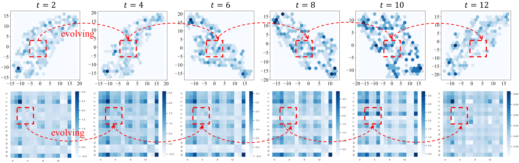
We compare the short (12 steps) and long (288 steps) term prediction curves between STSGCN, AGCRN, and our TrendGCN on a snapshot of the test data of four datasets, as shown in Fig. 8. We observe that our proposed TrendGCN can significantly bridge the trend discrepancy between prediction and ground truth for both short-term and long-term prediction, which confirms our intuition. In particular, for the fast-varying periods (dashed boxes), the predictions of TrendGCN are much closer to ground truth, which shows the stronger adaptive ability of TrendGCN for changes. Furthermroe, we visualize the learned dynamic adaptive graphs at the different time steps, aiming to discuss the interpretation of TrendGCN. For better visualization, we randomly select 16 nodes on PEMS04 dataset, as shown in Fig. 9. We have the following observations: 1) Although many methods using pre-defined graphs (static) have achieved comparable performance, they generally face the problem of data sparsity which harms the propagation of model’s gradient significantly; 2) Dynamic adaptive graphs can flexibly capture the complex spatial-temporal dependencies between all nodes at different time steps.
5.10. Graph Construction Discussion
We propose a unified scheme (see Eq. 2) to effectively couple the spatial (node-wise) and temporal (time-wise) embeddings through a gate module and use the integrated embeddings to construct graphs changing over time. The choices of can be the same or different. Here, four widely-used combinations with are discussed as follows:
| (17) | ||||
As can be seen in Fig. 7, we derive the following findings: (1) The default setting of in TrendGCN achieves optimal performance (see Table 2), which signifies the equal importance of homogeneous and heterogeneous interactions in the spatial-temporal domains. (2) TrendGCN is not sensitive to the choices of (the color bars are almost the same height) which further verifies our method enhances the robustness of traffic forecasting.
6. Conclusions and Future Work
In this paper, we proposed TrendGCN, a novel model for traffic forecasting that extends the flexibility of GCNs and the distribution-preserving capacity of generative and adversarial loss. Our approach addresses the challenges of capturing dynamics and maintaining robustness by introducing dynamic adaptive graph generation and adversarial dynamic trend alignment. Extensive experiments on six benchmarks and theoretical analyses demonstrate the superiority of TrendGCN. For further work, we will study the following two aspects: 1) investigating stronger methods to capture dynamic spatial-temporal dependencies, e.g., the mixture of experts (MoE); 2) exploring more effective approaches to enhance the robustness of traffic forecasting, e.g., taking higher-order derivatives of time series.
7. Acknowledgments
This work was partially supported by the National Natural Science Foundation of China (No. 62276099).
References
- (1)
- Bai et al. (2019) Lei Bai, Lina Yao, Salil S Kanhere, Xianzhi Wang, and Quan Z Sheng. 2019. STG2seq: spatial-temporal graph to sequence model for multi-step passenger demand forecasting. In Proceedings of the International Joint Conference on Artificial Intelligence. AAAI Press, Palo Alto, CA USA, 1981–1987.
- Bai et al. (2020) Lei Bai, Lina Yao, Can Li, Xianzhi Wang, and Can Wang. 2020. Adaptive graph convolutional recurrent network for traffic forecasting. In Advances in Neural Information Processing Systems. MIT Press, 17804–17815.
- Bai et al. (2018) Shaojie Bai, J Zico Kolter, and Vladlen Koltun. 2018. An empirical evaluation of generic convolutional and recurrent networks for sequence modeling. In International Conference on Learning Representations Workshop.
- Cao et al. (2020) Defu Cao, Yujing Wang, Juanyong Duan, Ce Zhang, Xia Zhu, Congrui Huang, Yunhai Tong, Bixiong Xu, Jing Bai, Jie Tong, and Qi Zhang. 2020. Spectral temporal graph neural network for multivariate time-series forecasting. Advances in Neural Information Processing Systems (2020), 17766–17778.
- Chen et al. (2023) Ling Chen, Donghui Chen, Zongjiang Shang, Binqing Wu, Cen Zheng, Bo Wen, and Wei Zhang. 2023. Multi-scale adaptive graph neural network for multivariate time series forecasting. IEEE Transactions on Knowledge and Data Engineering (2023).
- Chen et al. (2021) Yuzhou Chen, Ignacio Segovia, and Yulia R Gel. 2021. Z-GCNETs: Time zigzags at graph convolutional networks for time series forecasting. In International Conference on Machine Learning. 1684–1694.
- Choi et al. (2022) Jeongwhan Choi, Hwangyong Choi, Jeehyun Hwang, and Noseong Park. 2022. Graph neural controlled differential equations for traffic forecasting. In Proceedings of the AAAI Conference on Artificial Intelligence, Vol. 36. AAAI Press, Palo Alto, CA USA, 6367–6374.
- Chung et al. (2014) Junyoung Chung, Caglar Gulcehre, KyungHyun Cho, and Yoshua Bengio. 2014. Empirical evaluation of gated recurrent neural networks on sequence modeling. In Advances in Neural Information Processing Systems Workshop. MIT Press.
- Dai et al. (2019) Zihang Dai, Zhilin Yang, Yiming Yang, Jaime Carbonell, Quoc V Le, and Ruslan Salakhutdinov. 2019. Transformer-xl: Attentive language models beyond a fixed-length context. In Proceedings of the Annual Meeting of the Association for Computational Linguistics. 2978–2988.
- Diao et al. (2019) Zulong Diao, Xin Wang, Dafang Zhang, Yingru Liu, Kun Xie, and Shaoyao He. 2019. Dynamic spatial-temporal graph convolutional neural networks for traffic forecasting. In Proceedings of the AAAI conference on artificial intelligence, Vol. 33. AAAI Press, Palo Alto, CA USA, 890–897.
- Fang et al. (2021) Zheng Fang, Qingqing Long, Guojie Song, and Kunqing Xie. 2021. Spatial-temporal graph ode networks for traffic flow forecasting. In Proceedings of the ACM SIGKDD International Conference on Knowledge Discovery & Data Mining. Association for Computing Machinery, New York, NY, USA, 364–373.
- Geng et al. (2019) Xu Geng, Yaguang Li, Leye Wang, Lingyu Zhang, Qiang Yang, Jieping Ye, and Yan Liu. 2019. Spatiotemporal multi-graph convolution network for ride-hailing demand forecasting. In Proceedings of the AAAI Conference on Artificial Intelligence. AAAI Press, Palo Alto, CA USA, 3656–3663.
- Guo et al. (2019) Shengnan Guo, Youfang Lin, Ning Feng, Chao Song, and Huaiyu Wan. 2019. Attention based spatial-temporal graph convolutional networks for traffic flow forecasting. In Proceedings of the AAAI Conference on Artificial Intelligence. AAAI Press, Palo Alto, CA USA, 922–929.
- Guo et al. (2021) Shengnan Guo, Youfang Lin, Huaiyu Wan, Xiucheng Li, and Gao Cong. 2021. Learning dynamics and heterogeneity of spatial-temporal graph data for traffic forecasting. IEEE Transactions on Knowledge and Data Engineering (2021).
- Haidar et al. (2019) Md Haidar, Mehdi Rezagholizadeh, et al. 2019. Textkd-GAN: Text generation using knowledge distillation and generative adversarial networks. In Canadian conference on artificial intelligence. 107–118.
- Huang et al. (2020) Rongzhou Huang, Chuyin Huang, Yubao Liu, Genan Dai, and Weiyang Kong. 2020. LSGCN: Long Short-Term Traffic Prediction with Graph Convolutional Networks. In Proceedings of the International Joint Conference on Artificial Intelligence. AAAI Press, Palo Alto, CA USA, 2355–2361.
- Jiang et al. (2020) Juyong Jiang, Jie Zhang, and Kai Zhang. 2020. Cascaded semantic and positional self-attention network for document classification. In Conference on Empirical Methods in Natural Language Processing. Association for Computational Linguistics, 669–677.
- Jiang et al. (2021) Renhe Jiang, Du Yin, Zhaonan Wang, Yizhuo Wang, Jiewen Deng, Hangchen Liu, Zekun Cai, Jinliang Deng, Xuan Song, and Ryosuke Shibasaki. 2021. DL-Traff: Survey and benchmark of deep learning models for urban traffic prediction. In Proceedings of the ACM International Conference on Information & Knowledge Management. Association for Computing Machinery, New York, NY, USA, 4515–4525.
- Jiang and Luo (2021) Weiwei Jiang and Jiayun Luo. 2021. Graph neural network for traffic forecasting: A Survey. arXiv (2021).
- Khaled et al. (2022) Alkilane Khaled, Alfateh M Tag Elsir, and Yanming Shen. 2022. TFGAN: Traffic forecasting using generative adversarial network with multi-graph convolutional network. Knowledge-Based Systems 249 (2022), 108990.
- Lan et al. (2022) Shiyong Lan, Yitong Ma, Weikang Huang, Wenwu Wang, Hongyu Yang, and Pyang Li. 2022. DSTAGNN: Dynamic Spatial-Temporal Aware Graph Neural Network for Traffic Flow Forecasting. In International Conference on Machine Learning. PMLR, 11906–11917.
- Li et al. (2023) Fuxian Li, Jie Feng, Huan Yan, Guangyin Jin, Fan Yang, Funing Sun, Depeng Jin, and Yong Li. 2023. Dynamic Graph Convolutional Recurrent Network for Traffic Prediction: Benchmark and Solution. ACM Transactions on Knowledge Discovery from Data (TKDD) 17, 1 (2023).
- Li and Zhu (2021a) Mengzhang Li and Zhanxing Zhu. 2021a. Spatial-temporal fusion graph neural networks for traffic flow forecasting. In Proceedings of the AAAI Conference on Artificial Intelligence. AAAI Press, Palo Alto, CA USA, 4189–4196.
- Li and Zhu (2021b) Mengzhang Li and Zhanxing Zhu. 2021b. Spatial-temporal fusion graph neural networks for traffic flow forecasting. In Proceedings of the AAAI Conference on Artificial Intelligence, Vol. 35. AAAI Press, Palo Alto, CA USA, 4189–4196.
- Li et al. (2018) Yaguang Li, Rose Yu, Cyrus Shahabi, and Yan Liu. 2018. Diffusion convolutional recurrent neural network: Data-driven traffic forecasting. In International Conference on Learning Representations.
- Ma et al. (2017) Xiaolei Ma, Zhuang Dai, Zhengbing He, Jihui Ma, Yong Wang, and Yunpeng Wang. 2017. Learning traffic as images: A deep convolutional neural network for large-scale transportation network speed prediction. Sensors 17, 4 (2017), 818.
- SHI et al. (2015) Xingjian SHI, Zhourong Chen, Hao Wang, Dit-Yan Yeung, Wai-kin Wong, and Wang-chun WOO. 2015. Convolutional LSTM network: A machine learning approach for precipitation nowcasting. In Advances in Neural Information Processing Systems. MIT Press, 802–810.
- Song et al. (2020) Chao Song, Youfang Lin, Shengnan Guo, and Huaiyu Wan. 2020. Spatial-temporal synchronous graph convolutional networks: A new framework for spatial-temporal network data forecasting. In Proceedings of the AAAI Conference on Artificial Intelligence. AAAI Press, Palo Alto, CA USA, 914–921.
- Thomas N. Kipf (2017) Max Welling Thomas N. Kipf. 2017. Semi-supervised classification with graph convolutional networks. In International Conference on Learning Representations.
- Wang et al. (2021) Zhengwei Wang, Qi She, and Tomas E Ward. 2021. Generative adversarial networks in computer vision: A survey and taxonomy. ACM Computing Surveys (CSUR) 54, 2 (2021), 1–38.
- Williams and Hoel (2003) Billy M Williams and Lester A Hoel. 2003. Modeling and forecasting vehicular traffic flow as a seasonal ARIMA process: Theoretical basis and empirical results. Journal of transportation engineering 129, 6 (2003), 664–672.
- Wu et al. (2004) Chun-Hsin Wu, Jan-Ming Ho, and Der-Tsai Lee. 2004. Travel-time prediction with support vector regression. IEEE Transactions on Intelligent Transportation Systems 5, 4 (2004), 276–281.
- Wu et al. (2020b) Sifan Wu, Xi Xiao, Qianggang Ding, Peilin Zhao, Ying Wei, and Junzhou Huang. 2020b. Adversarial sparse transformer for time series forecasting. Advances in Neural Information Processing Systems (2020), 17105–17115.
- Wu et al. (2021) Zonghan Wu, Shirui Pan, Fengwen Chen, Guodong Long, Chengqi Zhang, and Philip S. Yu. 2021. A comprehensive survey on graph neural networks. IEEE Transactions on Neural Networks and Learning Systems 32, 1 (2021), 4–24.
- Wu et al. (2020a) Zonghan Wu, Shirui Pan, Guodong Long, Jing Jiang, Xiaojun Chang, and Chengqi Zhang. 2020a. Connecting the dots: multivariate time series forecasting with graph neural networks. In Proceedings of the ACM SIGKDD International Conference on Knowledge Discovery & Spec- tral temporal graph neural network for multivariate time- series forecasting. Association for Computing Machinery, 753–763.
- Wu et al. (2019) Zonghan Wu, Shirui Pan, Guodong Long, Jing Jiang, and Chengqi Zhang. 2019. Graph WaveNet for deep spatial-temporal graph modeling. In Proceedings of the International Joint Conference on Artificial Intelligence. AAAI Press, 1907–1913.
- Yoon et al. (2019) Jinsung Yoon, Daniel Jarrett, and Mihaela van der Schaar. 2019. Time-series generative adversarial networks. In Advances in Neural Information Processing Systems. 5508–5518.
- Yu et al. (2018) Bing Yu, Haoteng Yin, and Zhanxing Zhu. 2018. Spatio-temporal graph convolutional networks: A deep learning framework for traffic forecasting. In Proceedings of the International Joint Conference on Artificial Intelligence. AAAI Press, Palo Alto, CA USA, 3634–3640.
- Yu et al. (2022) Hongyuan Yu, Ting Li, Weichen Yu, Jianguo Li, Yan Huang, Liang Wang, and Alex Liu. 2022. Regularized Graph Structure Learning with Semantic Knowledge for Multi-variates Time-Series Forecasting. In Proceedings of the Thirty-First International Joint Conference on Artificial Intelligence. AAAI Press, 2362–2368.
- Yu et al. (2017) Haiyang Yu, Zhihai Wu, Shuqin Wang, Yunpeng Wang, and Xiaolei Ma. 2017. Spatiotemporal recurrent convolutional networks for traffic prediction in transportation networks. Sensors 17, 7 (2017), 1501.
- Zhang et al. (2020) Qi Zhang, Jianlong Chang, Gaofeng Meng, Shiming Xiang, and Chunhong Pan. 2020. Spatio-Temporal Graph Structure Learning for Traffic Forecasting. Proceedings of the AAAI Conference on Artificial Intelligence 34, 01 (2020), 1177–1185.
- Zhang et al. (2021) Yuxuan Zhang, Senzhang Wang, Bing Chen, Jiannong Cao, and Zhiqiu Huang. 2021. TrafficGAN: Network-scale deep traffic prediction with generative adversarial nets. IEEE Transactions on Intelligent Transportation Systems 22, 1 (2021), 219–230.
- Zheng et al. (2020) Chuanpan Zheng, Xiaoliang Fan, Cheng Wang, and Jianzhong Qi. 2020. GMAN: A graph multi-attention network for traffic prediction. In Proceedings of the AAAI Conference on Artificial Intelligence. AAAI Press, Palo Alto, CA USA, 1234–1241.
- Zivot and Wang (2006) Eric Zivot and Jiahui Wang. 2006. Vector autoregressive models for multivariate time series. Modeling financial time series with S-PLUS® (2006), 369–413.