Compressing (Multidimensional) Learned Bloom Filters

Kraska et al. [8] first suggested the idea of replacing indexes with deep learning models. Since this premise, a plethora of papers focus on improving traditional one-dimensional [4, 6, 7] and also multidimensional indexes [3, 5] with learned models. Since the idea of replacing a traditional Bloom filter [2] with a classification model [8], several improvements have been proposed. For instance, Vaidya et al. [11] use multiple more accurate learned filters based on classification score segments. Mitzenmacher [10] proposes a new sandwiched learned Bloom filter, including two surrounding Bloom filters for improved performance. Differently, Macke et al. [9] focus on extending the learned Bloom filter and show the benefits of having such an index for multidimensional data. Compressing the input of deep learning models has also been investigated for learned cardinality estimators. NeuroCard [12] uses a variable byte compression of columns to improve the proposed cardinality estimator. In our experiments, we compare only with the multidimensional learned filter since ideas like partitioning or sandwiching are orthogonal and can be used in combination with our approach.

Bloom filters are space-efficient data structures, used to test the existence of an element in a given dataset. Their probabilistic nature enforces the guarantees of no false negatives and tunable false positive rates. More specifically, a Bloom filter is an $m$ bit array (initially all bits are set to $0$), requiring $h$ well-defined hash functions. Upon adding an element, each of the $h$ hash functions maps the element to a position in the $m$ bit array and sets the bit to $1$. Evidently, the adaptation of a Bloom filter for multidimensional data would require indexing of all possible combinations of column values, to be able to accurately decide on the presence of subsets of values.

As an example for multidimensional data, consider a dataset containing vehicle information for a car rental agency. For simplicity, let us consider that the dataset has only three columns, the name of the car, the fuel type, and information on whether the car has been rented out. Intuitively, indexing multidimensional data would lead to a more comprehensive Bloom filter since the filter needs to answer membership queries involving subsets of the original records. As an example, considering the vehicles dataset described above, checking if there is an available car that runs on diesel can be done by querying for (${}?$,diesel,true) where "$?$" is a placeholder for any value. To answer this query, the Bloom filter needs to index all subsets of column values for a particular entry, including the ones where the column values are not specified, i.e., queries of the type ($?$,fuel_type,rented_out). Thus, the size of the Bloom filter will be directly affected by the possible combinations of co-occurring attributes that need to be covered by the index. On the other hand, when considering learned Bloom filters over multidimensional data, the model parameters are directly affected by the input dimensions, i.e., the distinct values of the columns. Hence, datasets in which columns have many distinctive values can result in higher memory consumption of the learned Bloom filter, although the space consumption will be still lower compared to traditional Bloom filter implementations [8, 9].

The number of inputs and their distinct values have a direct impact on the model parameters and, thus, the size of the model. One way to provide the inputs to the model is to use an embedding layer on every column. To accomplish this, proper mapping of string data to an integer value is performed for every column. However, the size of the embedding matrix will scale linearly with the number of unique values per column. Thus, even for a column with $10^{5}$ unique values, when using a $32$-dimensional embedding, the embedding matrix would take around $12.8$MB of space which is already much larger than a normal Bloom filter. By applying our proposed input compression, we aim at drastically reducing this space consumption.

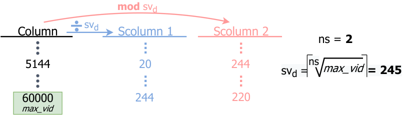
Consider a relation $R$ where $c_{1}$, $\dots$, $c_{n}$ represent columns with $v(c_{1})$, $\dots$, $v(c_{n})$ unique values. The main idea is to split a column into several subcolumns, together having fewer dimensions than the original column, contributing to a smaller encoding of the input and, thus, a smaller model size. The number of subcolumns is chosen based on the number of distinct column values, with the goal of smaller input dimensionality. For example, if the number of values for column $c_{i}$ is $v(c_{i})=10000$, two subcolumns are sufficient to efficiently compress the original column values whereas for a column with $10$ million unique values three or more subcolumns would be required to train the model. Our compression is based on the observation that we can reduce the input dimensionality by dividing the column values with a specific divisor. More specifically, to apply the encoding, we first identify the number of subcolumns $ns$ that a column should be split into. Then, we set as a divisor $sv_{d}$ to be the $ns^{th}$ root of the number of distinct values of the column, i.e., $sv_{d}\!=\left\lceil\!\sqrt[ns]{max\_vid\ }\ \right\rceil$. For compressing the column value $x$, we determine the quotient $sv_{q}$ and reminder $sv_{r}$ when dividing the value $x$ with $sv_{d}$. If $ns>2$, we repeat the same procedure for $x=sv_{q}$ and $max\_vid=max\_sv_{q}$, at the end reaching $ns$ subcolumns.

As an example, consider the column represented in Figure 1. As depicted, the number of distinct values for the column is $max\_vid=60000$ and we want to compress the value $x=5144$. If we want to split the column into two subcolumns, i.e., $ns=2$, then as the divisor we get $sv_{d}=245$ by calculating the squared root of $max\_vid$. Thus, the value $x=5144$ will be compressed in $sv_{q}=20$ and $sv_{r}=244$. In this case, all column values are split into two subvalues having maximal values $sv_{d}$ and $sv_{d}-1$. Through the compression, we reduce the number of dimensions needed to encode the input from $60000$ to $489$. When considering a $32$-dimensional embedding, we reduce the size of the embedding matrix from $7.8$MB to approximately $0.06$MB, which is a substantial space reduction.

We perform the compression over every column for which $v(c_{i})$ is greater than a compression threshold $\theta$. Unlike previous learned multidimensional Bloom filters, which encode the structure of the column through embeddings, we also allow a one-hot encoding in cases where the column has been already compressed to a smaller dimension and embedding matrices are no longer necessary.

Evidently, the proposed input compression would affect not only the model size but also the model accuracy. More specifically, parameter $ns$, which determines the number of subcolumns a column needs to be split into, allows a tradeoff between the model size and model accuracy. By increasing $ns$, although the unique column values are decreased, the number of input columns is increased. Consequently, the learning of the model will be negatively affected since it would need to learn across multiple columns with increased interconnection. Thus, we carefully set both $ns$ and the compression threshold $\theta$ for achieving an acceptable tradeoff.

References

- [1] . State of new york. vehicle, snowmobile, and boat registrations. catalog.data.gov/dataset/vehicle-snowmobile-and-boat-registrations, . Accessed: 2021-09-15.
- [2] Burton H. Bloom. Space/time trade-offs in hash coding with allowable errors. Commun. ACM, 13(7):422–426, 1970.
- [3] Angjela Davitkova, Evica Milchevski, and Sebastian Michel. The ml-index: A multidimensional, learned index for point, range, and nearest-neighbor queries. In EDBT, pages 407–410. OpenProceedings.org, 2020.
- [4] Jialin Ding, Umar Farooq Minhas, Jia Yu, Chi Wang, Jaeyoung Do, Yinan Li, Hantian Zhang, Badrish Chandramouli, Johannes Gehrke, Donald Kossmann, David B. Lomet, and Tim Kraska. ALEX: an updatable adaptive learned index. In SIGMOD Conference, pages 969–984. ACM, 2020.
- [5] Jialin Ding, Vikram Nathan, Mohammad Alizadeh, and Tim Kraska. Tsunami: A learned multi-dimensional index for correlated data and skewed workloads. Proc. VLDB Endow., 14(2):74–86, 2020.
- [6] Paolo Ferragina and Giorgio Vinciguerra. The pgm-index: a fully-dynamic compressed learned index with provable worst-case bounds. Proc. VLDB Endow., 13(8):1162–1175, 2020.
- [7] Andreas Kipf, Ryan Marcus, Alexander van Renen, Mihail Stoian, Alfons Kemper, Tim Kraska, and Thomas Neumann. Radixspline: a single-pass learned index. In aiDM@SIGMOD, pages 5:1–5:5. ACM, 2020.
- [8] Tim Kraska, Alex Beutel, Ed H. Chi, Jeffrey Dean, and Neoklis Polyzotis. The case for learned index structures. In SIGMOD Conference, pages 489–504. ACM, 2018.
- [9] Stephen Macke, Alex Beutel, Tim Kraska, M. Sathiamoorthy, D. Cheng, and Ed H. Chi. Lifting the curse of multidimensional data with learned existence indexes. In ML for Systems@NeurIPS, 2018.
- [10] Michael Mitzenmacher. A model for learned bloom filters and optimizing by sandwiching. In NeurIPS, pages 462–471, 2018.
- [11] Kapil Vaidya, Eric Knorr, Tim Kraska, and Michael Mitzenmacher. Partitioned learned bloom filter. CoRR, abs/2006.03176, 2020.
- [12] Zongheng Yang, Amog Kamsetty, Sifei Luan, Eric Liang, Yan Duan, Xi Chen, and Ion Stoica. Neurocard: One cardinality estimator for all tables. Proc. VLDB Endow., 14(1):61–73, 2020.