Boltzmann equations for astrophysical
Stochastic Gravitational Wave Backgrounds
scattering off of massive objects
Abstract
The goal of this work is to present a set of coupled Boltzmann equations describing the intensity and polarisation Stokes parameters of the SGWB. Collision terms (as discussed e.g. in Ref. [1]) which account for gravitational Compton scattering off of massive objects, are also included. This set resembles that for the CMB Stokes parameters, but the different spin nature of the gravitational radiation and the physics involved in the scattering process determine crucial differences. In the case of gravitational Compton scattering, due to the Rutherford angular dependence of the cross section, all the SGWB intensity multipoles of order are scattered out, therefore producing outgoing intensity anisotropies of any order if they are present in the incoming radiation. On the other hand, as already outlined in [1], SGWB linear polarisation modes can be expanded in a basis of spherical harmonics with and . This means that SGWB polarisation modes can be generated from unpolarised anisotropic radiation only with , therefore requiring at least a hexadecapole anisotropy () in the incoming intensity. Assuming a simplified toy model where scattering targets are localised in a small redshift range, we solve analytically the set of coupled Boltzmann equations to get explicit expressions for the intensity and polarisation angular power spectra. We confirm the contribution of the gravitational Compton scattering to the SGWB anisoptropies is extremely small for collisions with massive compact objects (BH and SMBH) in the frequency range of current and upcoming surveys. The system of coupled Boltzmann equations presented here provides a way to accurate estimate the total amount of anisotropies generated by multiple SGWB scattering processes off of massive objects, as well as the interplay between polarisation and intensity, during the GW propagation across the LSS of the universe. These results will be useful for the full treatment of the astrophysical SWGB anisotropies in view of upcoming gravitational waves observatories.
1 Introduction
The recent direct observations of Gravitational Wave (GW) signals [2, 3, 4, 5, 6, 7, 8, 9, 10, 11] have opened a new exciting era for astronomical and cosmological studies. The increase in sensitivity of current and upcoming detectors [12, 13, 14, 15, 16], both ground-based (e.g. the Laser Interferometer Gravitational Observatory, LIGO11 1 https://www.ligo.caltech.edu/, the VIRGO interferometer22 2 https://www.virgo-gw.eu/, the Kamioka Gravitational Wave Detector, KAGRA33 3 https://gwcenter.icrr.u-tokyo.ac.jp/en/, the Einstein Telescope, ET44 4 http://www.et-gw.eu, the Cosmic Explorer, CE55 5 https://cosmicexplorer.org/), and space-based (e.g. the Laser Interferometer Space Antenna, LISA66 6 https://www.lisamission.org/, and the Deci-hertz Interferometer Gravitational wave Observatory, DECIGO77 7 https://decigo.jp/index_E.html) will provide measurements of the Stochastic Gravitational Wave Background (SGWB) of both astrophysical and cosmological origins. In this context, a complete characterisation of the astrophysical SGWB and its evolution is crucial to distinguish it from the cosmological SGWB and obtain fundamental information about the very early universe. In particular, the analysis of the anisotropies in intensity (e.g. [17]) and polarisation (e.g. [18, 19]) of the latter would reveal the details of different physical processes in the inflationary era. The study of the SGWB intensity [20, 21, 22, 23, 24, 25, 26, 27, 28, 29, 30, 31, 32, 33, 34, 35] has been performed so far with approaches similar to those used for the Cosmic Microwave Background (CMB): its evolution is described by a phase-space distribution function obeying the collisionless Boltzmann equation in a background perturbed by the Large Scale Structure (LSS) of the universe [36, 37, 38, 39, 40]. This approximation applies in the so-called geometrical optics limit [41, 42, 43, 44, 45], i.e. when the GW wavelengths are much smaller than the typical spatial scale on which the perturbed background varies. As such, on cosmological scales, higher frequency gravitons behave as effectively spin-2 massless particles freely moving along geodesics. However, regarding the collisionless aspect of this treatment, as pointed out by Ref. [1], in the proximity of compact or extended massive objects, such as stars or black holes, graviton wavelengths could be much larger than the scale of variation of the spacetime generated by such structures, and wave effects, producing SWGB polarisation, need to be accounted for. In this respect, Ref. [1] has included the emissivity term in the Boltzmann equation of the SGWB intensity, but neglected the collision term, under the reasonable assumption that scattering effects, and the resultant SGWB polarisation, can be computed discarding the back reaction of polarisation on intensity.
In this work we present a set of Boltzmann equations for both the SGWB intensity and polarisation, with collision terms able to couple the system equations by including the SGWB scattering off of massive structures. To this aim, we exploit an approach similar to the treatment of CMB photons [46, 47, 48, 49, 50], where both the incoming and the scattered photons are considered free fields and the interaction term is a function of them [49]. In this case we consider the so-called Born approximation, i.e. we assume the GW propagation and scattering processes as characterised by two different length scales, the mean free path and the scattering length, with the assumption that, for weak enough couplings, the former is much larger than the latter. Under these hypotheses, for the gravitational scattering from massive objects, in the SGWB Boltzmann equations we consider as collision source the so-called Compton graviton-scalar scattering in the low-energy limit [51, 52, 53, 54, 55].
This paper is organised as follows: in Sec. 2 we report the definitions of the density matrix and Stokes parameters for GW backgrounds; in Sec. 3 we review the main features of the Compton cross-section entering the RHS of the collisional Boltzmann equations, in the case of the scattering of gravitons off of massive objects. We highlight the results obtained in the literature (e.g. [56, 1, 53, 54, 55]) and used in our computations; in Sec. 4 we derive the full set of Boltzmann equations for the Stokes parameters of GW backgrounds; in Sec. 5 we analyse the main features of the scattered SGWB intensity and polarisation anisotropies; in Sec. 6 we present and discuss the solution for the intensity and polarisation angular power spectra in the case of a simplified, toy-model scenario; finally, in the last Section we draw our conclusions.
2 Density matrix and Stokes parameters for gravitational radiation
The gravitational Stokes parameters (e.g. [43, 57, 58, 59]) provide, in analogy to the electromagnetic case, a way to completely characterise the intensity and polarisation content of the SGWB. The standard plane wave expansion of a generic GW, , in the so-called transverse traceless gauge, is given by
| (2.1) |
where is the unit sphere for the angular integral, the unit vector is the propagation direction, and is the basis for transverse-traceless tensors such that () where and are two unit vectors with a fixed spherical coordinate system. As the observed is real, one has a relation for the complex conjugate: . When replacing the direction , one has (even parity) and (odd parity). The covariance matrix, , between two polarisation modes, and , is given in terms of the GW Stokes parameters, , , , , as [57]:
| (2.2) |
where
| (2.3) | ||||
| (2.4) | ||||
| (2.5) | ||||
| (2.6) |
From now on, we omit the -dependence for simplicity. The symbol represents the ensemble average for a superposition of stationary incoherent waves, and is the delta function on the unit sphere. The parameter represents the total intensity of the SGWB, and are related to its linear polarisation, and to the circular polarisation. When the basis vectors, and , are rotated around the propagation direction, , by an angle , the parameters and are invariant (spin 0), while the combinations transform as , i.e. they are objects of spin [60].
Eq. (2.2) represents the so-called density matrix, in the linear polarisation basis , of an ensemble of gravitons in mixed state, and can be written in short notation as:
| (2.7) |
where is the identity matrix, and are the Pauli spin matrices. Thus the density matrix for an ensemble of gravitons contains the same information as the four Stokes parameters, and the time evolution of the density matrix provides the time evolution of the system.
In the considered quasi-classical limit, and for astrophysical SGWB, one can assume that the graviton phase-space distribution function, (treated in Sec. 4 below), is given by the Wigner distribution function, i.e. the Wigner transform of the density matrix [61, 62, 63, 64, 65, 66, 67]. Under such a hypothesis, in the following we will assume that, as for CMB photons, perturbations to the graviton density matrix correspond to perturbations to the classical gravitational Stokes parameters describing the intensity and polarisation of the astrophysical SGWB, and behaving as phase-space distribution functions which obey the respective Boltzmann equation with a collision term given by the gravitational Compton scattering from massive objects in the low energy limit [53].
3 Compton graviton-scalar scattering in the low energy limit
The process of GW scattering off of compact and massive objects, treated as spin-0 quantities, has been studied since the sixties via several methods, both from quantum-mechanical [52, 54, 53] and classical [68, 51, 55, 56] perspectives. Here we review results in the literature (e.g. [56, 1, 53, 54, 55]), which in turn will enter the collision term in the RHS of the SGWB Boltzmann equations representing the real novelty of this work. In particular, we will consider the long wavelength/weak-field limit of gravitational Compton scattering, i.e. when the wavelength, , of the incoming wave is assumed to be much larger than the Schwarzschild radius, , of the scattering object of mass , i.e. [55]. We use units of and, in first approximation, neglect any possible angular momentum of the compact object since it has been suggested that, to first order in , gravitational waves do not exhibit angular-momentum-induced effects [56].
In particular, considering a gravitational wave with polarisation tensor hitting, from the direction , a compact object of mass and zero angular momentum, the differential cross section, in the TT gauge and in the rest frame of the object, is [56]
| (3.1) |
where is the outgoing polarisation of the wave, and is the angle between the incoming and outgoing directions.
In the so-called scattering plane geometry, one can decompose the polarisation basis in terms of a pair of unit vectors normal to the direction of propagation, for the vector in the scattering plane and for the vector normal to it, and write
| (3.2) |
Using a similar decomposition for the incoming polarisation tensor , and the relation between the “primed” and “unprimed” vectors in terms of the incoming direction :
| (3.3) |
one then obtains the relations
| (3.4) |
Finally, using Eqs. (3.1)-(3), one can derive the polarisation-summed cross section averaged over the initial polarisation states, (unpolarised incident GWs), and summed over the final states, [56, 1, 53, 54, 55]
| (3.5) |
However, here we are interested in investigating how the GW components and get modified in the scattering event. It comes out that, similarly to the electromagnetic case, the plus and cross amplitudes need to be multiplied by their respective factors in Eq. (3), but a polarisation-independent angular dependence is also present, such that
| (3.6) |
Note that, unlike the electromagnetic case, in gravitational wave scattering the helicity is not conserved and the scattering cross section is nonzero in the backward direction, implying the existence of a helicity-reversing amplitude [56, 55]. Moreover, Eq. (3) diverges as for small scattering angles, i.e. in the forward scattering direction. This feature is the gravitational equivalent of the Rutherford’s angular dependence in electromagnetism, and, as pointed out in Refs. [51, 69, 1, 52], it is related to the long range nature of the gravitational interaction, or, alternatively, to the non-linear nature of Einstein’s equations [54].
In this work, in order to fix this divergence, we follow and summarise in this Section the method proposed by Ref. [1] which introduces a natural cutoff scale on , in order to deal with a well-defined total cross-section of the process. In particular, as pointed out in Ref. [1], this is a standard procedure when considering Boltzmann equations for systems where long range interactions are involved, such as the Coulomb scattering in plasma (e.g. Ref. [70] and references therein). The cutoff scale comes from the observation that wave-like effects are non-negligible only within a region whose size is given by the square root of the Kretschmann scalar, , associated to the metric generated by the scattering object. Assuming this is well approximated by a Schwarzschild metric, one has , where is the distance from the centre of the object. Therefore, for wavelengths , i.e. , wave-effects are non-negligible. The region, defined by , around the scattering object, depends on both its size and the wavelength of the incoming GW. In the far-field regime, the relation between the scattering angle, , and the impact parameter, , of a graviton geodesic, is given by . Therefore, if an upper bound exists for , one can find a corresponding lower bound on . The idea proposed by Ref. [1] is to choose , so that the minimum value of the scattering angle is given by . Analogously, Ref. [1] provides also an upper bound for the impact parameter of compact objects, which translates in a lower bound . Moreover, assuming that for sources corresponding to black holes, wave effects occur in a region , implying , it follows that a limit for the observed and redshifted wavelength, , of a GW scattered by a massive object of mass at redshift , is given by
| (3.7) |
Thus, GWs with relatively small wavelengths are affected only by scattering due to small mass objects, while GWs with large receive contribution from massive objects as well. In Tab. 1 we summarise the scattering masses of compact sources which fall in the observational ranges of ongoing and upcoming GW experiments.
| Detector | Mass | ||
|---|---|---|---|
| LIGO/VIRGO | |||
| ET | |||
| LGWA | |||
| LISA | |||
| PTA |
Finally, adopting the above limits on the scattering angle and integrating Eq. (3) over the solid angle, one obtains the total cross-section:
| (3.8) |
where
| (3.9) |
4 SGWB Boltzmann equations with collision terms
In the quasi-classical limit, the general approach to describe the evolution of the SGWB, travelling across the LSS of the universe, passes through the graviton Wigner function, i.e. the graviton phase-space distribution function, , where denotes the spacetime coordinates, is the four-momentum, and is an affine parameter along the graviton trajectories. This distribution function follows the Boltzmann equation (e.g. [36, 37, 38]):
| (4.1) |
where is the Liouville operator, is the collision term representing the interaction between GW and massive objects, and is a source term due to emission processes from astrophysical and cosmological GW sources. Here, we are interested in evaluating, in the Born approximation, which contributes both to the SGWB intensity and polarisation, while we ignore the contribution from the emissivity term, [37, 1], and possible effects of graviton scattering with other particles (see e.g. [78, 38]).
The approach followed in this work is based on the analogy with the standard treatment of CMB anisotropies [46, 47, 50]. In particular, we use the fact that, in the photon propagation description, the vector radiative transfer equation (VRTE) - which describes the rate of change of the Stokes parameters - is formally equivalent to the Boltzmann equations for CMB intensity and polarisation (see e.g. [49]). We apply the same treatment to the GW Stokes parameters defined via the density matrix in Eq. (2.2), for which, as the system becomes classical, can be interpreted as its Wigner transform.
We therefore consider the GWs Stokes vector and write the Boltzmann equation as [48, 47, 46]
| (4.2) |
where is the conformal time, is the flux of the outgoing radiation, and defines the "optical" thickness, in this case due to graviton scattering, of the medium through which the gravitational radiation is propagating. The dot indicates derivative with respect to . In the case of gravitational waves incoming over a distribution of massive objects, the optical thickness is given by [1]:
| (4.3) |
for an initial conformal time . In the above equation, is the physical density of massive objects which incoming GWs are scattered off at a given epoch , is the scale factor of the universe, and is the total cross-section of Eq. (3.8). Note that here we work in a simplified scenario of incoherent scattering [1] assuming all the massive scatters to have the same mass . In principle, one could refine this approximation by integrating, over reasonable mass ranges, the R.H.S of Eq. (4.2) times a weighting function that describes the mass distribution of the objects. However, as we will see in Sec. 5, this will not affect the overall results of our analysis.
After scattering, the outgoing radiation is given by:
| (4.4) |
with and n the incident and outgoing directions, respectively. All the physics of the scattering process is described by the scattering matrix, , which connects the incoming and the outgoing Stokes vectors. We derive an explicit expression for it in terms of Spin Weighted Spherical Harmonics (SWSH), , with spin and order (see Appendix A and e.g. [79, 46]):
| (4.5) |
where we have included circular polarisation terms () and made explicit the dependence on scalar and spin weighted spherical harmonics:
| (4.6) |
Computation details are given in Appendix B. A quick inspection of the null terms in the structure of reveals that the circular polarisation is not generated by the gravitational Compton scattering for an incident SGWB background without an initial circular polarisation; this is a feature in common with Thomson scattering between electrons and CMB photons [56, 55, 49, 1]. However, we highlight here three crucial differences with the CMB Thomson scattering process:
- •
First, the gravitational Compton scattering matrix is characterised by the presence of the overall factor coming from the Rutherford’s type denominator of the cross-section, Eq. (3.1), which complicates the angular dependence as compared to the CMB case.
- •
Second, the presence of SWSH of order 4 in is expected since transform under rotations as spin-4 quantities, thus they have to be decomposed in terms of spin-4 weighted spherical harmonics:
(4.7) Instead, in the photon case, the linear polarisations are spin-2 quantities (see e.g. [48]), thus the CMB scattering matrix contains SWSH of [46]. This is related to the nature of the propagating field (spin-1 in the case of photons and spin-2 in the case of gravitons).
- •
Third, in we see terms of order (hexadecapole) in scalar and spin-weighted spherical harmonics (instead of the quadrupole, , that characterises CMB Thomson scattering); this is a consequence of the spin-0 nature of the intensity, , and, again, the spin-4 nature of the polarisation, , in the graviton case.
4.1 The perturbed Boltzmann equations for gravitational Stokes parameters
We can now insert the scattering matrix, of Eq. (4.5), into the Boltzmann equation (4.2), and expand it to first order in terms of graviton energy and polarisation vectors88 8 The approach of dealing with density matrices and distributions functions is completely different from the usual one of considering GWs as linear metric perturbations and solve for their evolution by linearising the Einstein’s equations. Therefore, the graviton ensemble described by the density matrix perturbed at first order in energy and polarisation vectors can represent GWs beyond the linear regime in terms of the standard theory of cosmological perturbations. to obtain the evolution equation of the gravitational Stokes parameters in an inhomogeneous universe. For the sake of simplicity, in the LHS (Liouville part) of the Boltzmann equations (4.2) we consider only linear scalar metric perturbations over a flat FLRW background and neglect possible tensor metric perturbations, in order to avoid double counting (unless separated in distinct frequency ranges such that the geometrical optics limit still holds) the tensor perturbations in the SGWB described by the phase-space distribution function, , travelling on top of the perturbed background. In the conformal Newtonian gauge, the line element reads:
| (4.8) |
where and are and functions of the spacetime. The metric perturbations generate fluctuations, , to the unperturbed graviton density matrix, :
| (4.9) |
where, is the comoving momentum modulus, represents the uniform and unpolarised GW density matrix such that , and is the linear perturbation of Eq. (2.2). Therefore we expand at linear order the Stokes vector , associated to the density matrix , and, following the approach of Ref. [49], we define the linear perturbations of the SGWB Stokes parameters as
| (4.10) |
In the following, for simplicity of notation we retain only the n dependence of all the quantities. In Section 6 we explicitly recall the full dependence when needed. The above quantities represents linear order fluctuations in the Stokes parameters conveniently scaled by the energy density of the background graviton distribution. To obtain the perturbed R.H.S of the SGWB Boltzmann equation, Eq. (4.2), we substitute Eq. (4.5) into Eq. (4.4) and perturb the Stokes vector, , at linear order in terms of the quantities defined in Eq. (4.10). Moreover, similarly to [1], we introduce the following integrals, making here the dependence on the SWSH explicit:
| (4.11) |
The above quantities can be interpreted as averages over all directions of the incoming intensity and polarisation, weighted by the Rutherford’s type factor, , and by SWSH with and . Note that the integrals are not evaluated on the whole solid angle, but they are limited by the restriction given by the cutoff . Finally, to obtain the full set of linear Boltzmann equations for GWs, we consider Eq. (4.8) and expand, up to first order in the scalar metric perturbations, the L.H.S of Eq. (4.2), obtaining the usual Liouville-like term as for the CMB photon distribution function99 9 In this treatment we are neglecting first order corrections to the cross-section due to bulk velocities of the massive objects and to their angular momentum (see e.g. [53]). (e.g. [80, 46, 37, 50]).
We recall here we are working under two different assumptions: the geometrical optics limit, i.e. GW wavelengths being much smaller than the typical spatial scale on which linear metric perturbations vary, and the Born approximation, i.e. the mean free path of gravitons scattered off by massive objects being much larger than the scattering length.
Finally, the final set of linear Boltzmann equations for the gravitational Stokes parameters of the astrophysical SGWB read as
Intensity equation:
|
|
(4.12) |
Linear polarisation equation:
|
|
(4.13) |
Circular polarisation equation:
|
|
(4.14) |
Here we have exploited the fact that the solution of Eq.(4.2) at zeroth order in perturbation theory is simply the background uniform unpolarised density matrix, i.e. the redshifted intensity, , associated to the monopole of the SGWB. This cancels out between the L.H.S and R.H.S of Eqs. (4.12)-(4.14).
This system of coupled equations appears rather complicated due to the scattering terms in the R.H.S which include SWSH with and , plus the Rutherford’s type factor hidden in the integrals of Eq. (4.11). However, a direct inspection of Eqs. (4.12)-(4.14) reveals some interesting physical features, as described below.
5 Intensity and polarisation anistropies of the astrophysical SGWB
In a reference frame where the scattered wave is propagating along the axis, one can expand the intensity of unpolarised incoming waves in the basis of spherical harmonics:
| (5.1) |
where the tilde indicates that quantities are computed in the aligned frame. The coefficients are related to the in a generic direction as (e.g. [81]):
| (5.2) |
In Eq. (5.2), the quantities represent the (complex-conjugate) elements of the Wigner-D matrix (e.g. [82]), connecting a frame to another one obtained by rotating the former by an angle along the -axis and an angle along the -axis.
In the -alinged frame, the scattered intensity and linear polarisations are given by (see Eq. (B.4) and e.g. [1]):
| (5.3) |
| (5.4) |
The Stokes parameter remains everywhere zero if the incoming radiation is initially circularly unpolarised. Note that, each multipole, , with in gives a null contribution to Eq. (5.3), as the integral over vanishes.
In Thomson scattering for photons, regardless of the anisotropies of the incident radiation, only the monopole and the quadrupole are affected by the process, while the other multipoles integrate to zero via the orthogonality of spherical harmonics (thus, they remain unchanged with respect to the incident field). However, we stress here this is no more true for the gravitational Stokes parameters, since the Rutherford’s type divergence, , causes all the incoming multipoles (with ) to be scattered, therefore producing outgoing anisotropies of any order if they are present in input.
Regarding , the factor makes the integral in Eq. (5.4) identically zero unless incident radiation has a non-vanishing components, which implies : at least an hexadecapole anisotropy is needed to generate polarisation form an initially unpolarised radiation.
We now estimate the order of magnitude of the R.H.S. of Eqs. (4.12)–(4.13), by evaluating the cross-section and the expected comoving density of the scattering targets.
Given an observed wavelength, only objects for which the condition Eq. (3.7) holds contribute to the scattering. For Stellar mass Black Holes (StBH) with typical masses , the wavelengths involved satisfy , where, in Eq. (3.7), we have assumed that the scattering happens at an average redshift . This means that the contribution of StBH ideally affects the observations of all current and upcoming surveys. We consider , which is inside the LIGO/VIRGO band (see Tab. 1). From Eq. (3.8), the total cross-section is
| (5.5) |
Following e.g. [83, 1], we estimate the number density of StBH in the local universe to be ; this implies that the overall pre-factor multiplying the R.H.S. of Eqs. (4.12)–(4.13) is extremely small, as one can visually inspect in Fig. 1, where we show the full-sky maps for the outgoing and Stokes parameters1010 10 We generally refer to “outgoing” radiation as the total contribution in the R.H.S. of Eqs. (4.12)-(4.14), i.e. with the incoming radiation subtracted., as listed in the fourth and fifth columns of Tab. 2.

The incident radiation (top left panel of Fig. 1) is assumed to be unpolarised and given by a pure intensity hexadecapole, with , of order-unity:
where indicate the angles at which the incoming radiation is observed in the laboratory frame.
Assuming a value of unity for the incoming intensity, the order-of-magnitude of the collision term is for the intensity and for the linear polarisations.
Thus, as expected, the collision term due to GWs Compton scattering off of massive objects appears to provide a very small contribution to the R.H.S of Boltzmann equations for gravitons, at least when the scattering is sourced by stellar mass BH. An order-of-magnitude estimate of the polarisation produced by scattering off of various astrophysical objects can be found in Ref. [1], where it is shown that the SGWB polarisation produced by massive scatters is smaller by several orders of magnitude than the intensity anisotropies, for almost all frequency bands of ongoing and upcoming detectors. Nonetheless, we remark that in this work we are not only interested in the total polarisation as in Ref. [1], but rather we focus on the presentation of the system of coupled Boltzmann equations for SGWB intensity and polarisation anisotropies, which provides a way to estimate the correct, albeit very small, interplay between the two.
Note that an azimuthally-symmetric (i.e. independent of ) incoming SGWB field with an hexadecapole intensity anisotropy will generate a polarisation in the plane between the incoming and outgoing directions which is real () and proportional to , as one can directly verify by using the definitions of the Wigner-D symbols, and then computing the integrals of Eqs. (5.3)-(5.4). This differs from the electromagnetic case, where only a quadrupole intensity anisotropy is needed to generate linear polarisation via Thomson scattering.
It is important to stress that the integrals of Eq. (5.3) and Eq. (5.4) are limited by the cutoff . Thus, the larger is the wavelength considered in the scattering process, the smaller is the value of . In Tab. 2 we list the values of the optical depth and the corresponding order-of-magnitude values of the collision term for intensity and polarisation at different , generated from scattering of order-unity unpolarised incoming radiation. For all the wavelengths, we have considered GW collisions with a population of stellar mass BHs with at .
Moreover, it is worth noticing that a decrease in does not make the scattered polarisation, Eq. (5.4), to diverge, as the integral converges for (the limit of the ratio in the integrand is finite and equal to for ). However, Eq. (5.3) is divergent for small scattering angles, which means that the collisional term in Eq. (4.12) grows with increasing .
Note that a full numerical solution of the system of coupled SGWB Boltzmann Eqs. (4.12)–(4.14), would be needed to provide an accurate estimate of the total amount of polarisation generated by multiple scattering processes off of massive objects, as well as its interplay with intensity anisotropies, during the SGWB propagation across the LSS of the universe; this however is beyond the purpose of this paper. Nevertheless, it would be interesting to solve the set of equations in a simplified scenario. In the next Section, we provide analytical expressions for the angular power spectrum of intensity and polarisation perturbations, assuming unpolarised incoming radiation scattered off a uniform distribution of targets located in a small redshift interval.
| R.H.S | R.H.S | Detector | |||
|---|---|---|---|---|---|
| LIGO/VIRGO, ET | |||||
| LGWA, LISA | |||||
| PTA | |||||
6 Intensity and polarisation angular power spectra: a toy model
Consider a flux of incoming gravitational radiation propagating since an initial time over a cosmological perturbed FLRW background. These gravitational waves are then scattered by a population of massive compact objects within a small interval of redshifts , and then freely propagate towards the observer at the present time . We can formally solve1111 11 Note that we ignore circular polarisation modes, as they are not sourced in the scattering process. Eqs. (4.12)-(4.13) by working in Fourier space:
| (6.1) |
| (6.2) |
where we have defined
and
Note that when not needed, we keep as implicit the dependence on the variable ensemble . We have further introduced , the cosine between the wavenumber k and the direction of propagation n.
As in the collisionless case (e.g. [37] for the case of intenisties anisotropies alone) we can write the formal solution of the Boltzmann equations as:
| (6.3) |
| (6.4) |
In both equations we have used the fact that the optical depth in Eq. (4.3) is zero at by definition. The first terms in the RHS carry the information about initial conditions, weighted by the exponential of the optical depth. We now assume that the initial net polarisation anisotropy of the incoming radiation at is zero, i.e. the two terms depending on in and are zero, as well as the term in Eq. (6.4). The function is called visibility function and its integral from to gives the probability that a GW is scattered by massive objects between the initial and present times (see [1]). We now consider a simplified case in which the scattering targets are well localised in a small redshift interval , such that the visibility function is non-vanishing only if . We can therefore assume that all the other quantities do not change significantly in that time interval and evaluate them at . In this way, since for (see Tab. 1) one has:
the integrals in the RHS of Eqs. (6.3)-(6.4) become respectively:
| (6.5) |
| (6.6) |
By decomposing the incoming intensity in spherical harmonics
and using the properties under rotations of Eq. (5.2) to compute the integrals over the incoming directions in a frame aligned along the -axis, we can rewrite the collision terms , in Eqs. (6.5)-(6.6) in a more useful form:
| (6.7) |
| (6.8) |
where we have defined
Here, and represent the cut off range as defined in Sec. 4.1, and are the Legendre and associated Legendre polynomials, respectively, and using their properties it is possible to show that .
For the sake of simplicity, we now neglect the scalar perturbations of the metric in the time interval as in this toy model we are interested in estimating the contribution, to the intensity and polarisation angular power spectra observed today, of the collision terms alone. Moreover, we assume that the initial distribution of perturbations in the SGWB intensity is statistically isotropic, , i.e. it is represented by a monopole at the initial time , such that different moments measured by the observer at comes only from projection effects.
We introduce the two-point correlation function of the initial intensity anisotropy in Fourier space as (e.g. [37])
| (6.9) |
with the initial power spectrum, carrying out information about the physical processes generating the SGWB.
The intensity angular power spectrum observed today at the spacetime point is then obtained by decomposing the RHS of Eqs. (6.3)-(6.4) in terms of scalar and spin-weighted spherical harmonics with , respectively:
| (6.10) |
| (6.11) |
where we have generally indicated with , with , the RHS of Eqs. (6.3)-(6.4). After some mathematical manipulations, summarised in Appendix C, the above equations can be rearranged to give:
| (6.12) |
| (6.13) |
Note the presence of the Wigner 3j symbols:
which are connected to the Clebsch-Gordan coefficients and satisfy the triangular relation , together with .
The expression of and are quite cumbersome, even in the simplified scenario considered. In both Eqs. (6.12)-(6.13), the summed indices come from the incoming intensity monopole at which is scattered at and projected to (,), while are related to the outgoing radiation freely propagating from and observed at . The sums are further regulated by the selection rules of the Wigner 3j symbols.
The terms between square brackets which multiply the integral over encapsulate the effect of collisions. More in details, Eq. (6.12) can be seen as the sum of three contributions, , related to the three terms in square brackets. The first term, multiplied by the exponential , refers to the initial radiation propagating without being scattered, the second term is the contribution to the intensity power spectrum from SGWB scattering at , while the last term represents the cross correlation between the two. Considering a single multipole at a time at , , it is easy to evaluate the fractional overall contribution from GW Compton scattering with respect to the unscattered radiation in the angular power spectrum:
| (6.14) |
We remark here that all the terms in Eq. (6.14) implicitly depend on the GW frequency (wavelength) through the Rutherford-divergent cross section , as already pointed out in the previous sections.
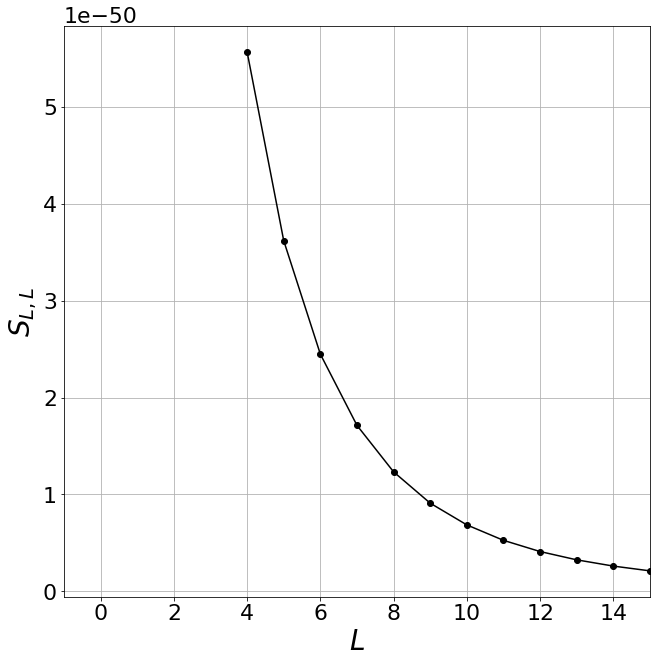
In the left panel of Fig. 2, we show as a function of the first 15 multipoles, for the case of a uniform distribution of stellar-mass black holes at with and . As expected, the contribution of the GW Compton scattering to the intensity angular power spectrum is extremely small. Moreover it drops rapidly when going to higher multipoles. We also observe that is dominated by the second term which arises from cross correlation between the incoming and scattered radiation.
The structure of Eq. (6.13) is very similar to Eq. (6.12), except for the presence of the three j symbols with . This is related to the spin 4-nature of and makes the term identically zero for , , as expected. The term in the square brackets of Eq. (6.13):
| (6.15) |
represents the order of magnitude of the polarisation generated by GW Compton scattering by massive objects. We can proceed as above and evaluate the contribution to the angular power spectrum for a single multipole, , at a time. In the right panel of Fig. 2 we show the value of of for , confirming that the amount of polarisation generated during a single scattering process is very small for wavelengths in the LIGO-VIRGO band, as already found in [1] using a different approach.
However, we stress here that the calculations presented in this section neglect scalar metric perturbations and their time derivative which affect the SGWB free-streaming from to . On the one hand, as pointed out in the literature (see e.g. [17]), metric perturbations produce intensity anisotropies of an even isotropic SGWB component. In turn, such intensity anisoptropies, changing in amplitude due to propagation on a perturbed background, enter the RHS of the coupled Boltzmann equations for intensity and polarisation, causing, at least via the change of during GW free-streaming among different collisions (but also with the generation of the terms), the change of the RHS in Eqs. (6.12)-(6.13), and therefore of the observed intensity and polarisation power spectra. On the other hand, despite we have worked with several simplifications, the formalism we developed here is completely general and independent of the initial conditions . Therefore our computation could be extended to the case of an angular-dependent initial intensity perturbation and to polarised incoming radiation. In principle, via our approach, one could also estimate the contribution of multiple scattering episodes by considering a series of independent collisions happening at different fixed redshift and assuming that the SGWB evolves freely between and .

7 Conclusions
In this paper we have provided, for the first time to date, a system of coupled Boltzmann equations describing the intensity and polarisation Stokes parameters of the astrophysical SGWB, including collision terms which account for gravitational Compton scattering off of massive objects. In analogy with Thomson scattering in the electromagnetic case, we have computed the full scattering matrix, Eq. (4.5), appearing in the collision term of the graviton Boltzmann equations in the low-energy limit of the graviton-scalar cross-section. The final set of equations, Eqs. (4.12)-(4.14), resembles that for the CMB Stokes parameters [49, 50, 46]; however, the different spin nature of the radiation and the physics involved in the scattering process determine crucial differences between photon and graviton stochastic backgrounds.
In particular, while photon Thomson scattering affects only anisotropies in the intensity of the incoming radiation with , due to orthogonality of spherical harmonics, in the case of gravitational Compton scattering with massive objects the Rutherford’s type term, , makes all multipoles (with ) to be scattered out, therefore producing outgoing anisotropies of any order if they are present in the intensity of the incident GW field.
Linear polarisation can be generated from unpolarised anisotropic radiation only with , which requires at least an hexadecapole anisotropy () in the incoming intensity; this is again a consequence of the fact that is a spin-4 quantity in the case of gravitons.
We have further provided an analytic solution for the angular power spectrum of intensity and polarisation anisotropies when the scattering targets are located in a small redshift range, under the assumption of unpolarised incoming monopole radiation and neglecting free-streaming effects due to metric scalar perturbations We explicitly computed the order of magnitude of the contribution of SGWB Compton scattering by massive objects to the intensity and polarisation power spectra as a function of the projected multipoles moments of the incoming radiation.
Our analysis confirms that the contribution of the gravitational Compton scattering to SGWB anisotropies is extremely small for collisions with massive compact objects (BH and SMBH) in the frequency range of current and upcoming surveys, as already found in previous studies with different methods [1]. This statement can be extended to other massive scatters as main sequence stars. However, in our simplified estimation of such contribution, we completely neglected effects sourced by the generation of further intensity and polarisation anisotropies during GW propagation on a perturbed FLRW background, which in turn enter the collision term in the RHS of the Boltzmann equations.
In conclusion, it is important to stress that the focus of this work relies on the set of coupled Boltzmann equations for SGWB intensity and polarisation Stokes parameters, which we present here for the first time in the literature. Beyond the simplified model described above, a full numerical integration of the coupled Eqs. (4.12)–(4.14) would provide a more accurate estimate of the total amount of anisotropies generated by multiple scattering processes off of massive objects, as well as the interplay between polarisation and intensity (including a polarised incoming background), during the SGWB propagation across the LSS of the universe. This will be investigated in future works.
Acknowledgments
CB and CC warmly thank Andrew Jaffe for very useful and interesting discussions since the initial concepts in 2006. LP ackwnoledges GBR and VB for useful comments and discussions. CB acknowledges support from the InDark INFN initiative. LP acknowledges support from the Czech Academy of Sciences under the grant number LQ100102101. LP and MC are partially supported by a 2019, 2020, 2021 and 2022 “Research and Education” grant from Fondazione CRT. The OAVdA is managed by the Fondazione Clément Fillietroz-ONLUS, which is supported by the Regional Government of the Aosta Valley, the Town Municipality of Nus and the “Unité des Communes valdôtaines Mont-Émilius”.
References
- [1] G. Cusin, R. Durrer and P.G. Ferreira, Polarization of a stochastic gravitational wave background through diffusion by massive structures, Phys. Rev. D 99 (2019) 023534 [1807.10620].
- [2] B.P. Abbott, R. Abbott, T.D. Abbott, M.R. Abernathy, F. Acernese, K. Ackley et al., Observation of Gravitational Waves from a Binary Black Hole Merger, Phys. Rev. Lett. 116 (2016) 061102 [1602.03837].
- [3] B.P. Abbott, R. Abbott, T.D. Abbott, F. Acernese, K. Ackley, C. Adams et al., GW170817: Observation of Gravitational Waves from a Binary Neutron Star Inspiral, Phys. Rev. Lett. 119 (2017) 161101 [1710.05832].
- [4] B.P. Abbott, R. Abbott, T.D. Abbott, F. Acernese, K. Ackley, C. Adams et al., Gravitational Waves and Gamma-Rays from a Binary Neutron Star Merger: GW170817 and GRB 170817A, ApJ 848 (2017) L13 [1710.05834].
- [5] R. Abbott, T.D. Abbott, S. Abraham, F. Acernese, K. Ackley, A. Adams et al., GWTC-2: Compact Binary Coalescences Observed by LIGO and Virgo during the First Half of the Third Observing Run, Physical Review X 11 (2021) 021053 [2010.14527].
- [6] The LIGO Scientific Collaboration, the Virgo Collaboration, the KAGRA Collaboration, R. Abbott, T.D. Abbott, F. Acernese et al., GWTC-3: Compact Binary Coalescences Observed by LIGO and Virgo During the Second Part of the Third Observing Run, arXiv e-prints (2021) arXiv:2111.03606 [2111.03606].
- [7] The LIGO Scientific Collaboration, the Virgo Collaboration, the KAGRA Collaboration, R. Abbott, T.D. Abbott, F. Acernese et al., The population of merging compact binaries inferred using gravitational waves through GWTC-3, arXiv e-prints (2021) arXiv:2111.03634 [2111.03634].
- [8] The LIGO Scientific Collaboration, the Virgo Collaboration, the KAGRA Collaboration, R. Abbott, H. Abe, F. Acernese et al., Tests of General Relativity with GWTC-3, arXiv e-prints (2021) arXiv:2112.06861 [2112.06861].
- [9] The LIGO Scientific Collaboration, the Virgo Collaboration, the KAGRA Collaboration, R. Abbott, H. Abe, F. Acernese et al., Constraints on the cosmic expansion history from GWTC-3, arXiv e-prints (2021) arXiv:2111.03604 [2111.03604].
- [10] F. Hernandez Vivanco, R. Smith, E. Thrane, P.D. Lasky, C. Talbot and V. Raymond, Measuring the neutron star equation of state with gravitational waves: The first forty binary neutron star merger observations, Phys. Rev. D 100 (2019) 103009 [1909.02698].
- [11] Z. Arzoumanian, P.T. Baker, H. Blumer, B. Bécsy, A. Brazier, P.R. Brook et al., The NANOGrav 12.5 yr Data Set: Search for an Isotropic Stochastic Gravitational-wave Background, ApJ 905 (2020) L34 [2009.04496].
- [12] M. Maggiore, C. Van Den Broeck, N. Bartolo, E. Belgacem, D. Bertacca, M.A. Bizouard et al., Science case for the Einstein telescope, J. Cosmology Astropart. Phys 2020 (2020) 050 [1912.02622].
- [13] J. Baker, T. Baker, C. Carbone, G. Congedo, C. Contaldi, I. Dvorkin et al., High angular resolution gravitational wave astronomy, arXiv e-prints (2019) arXiv:1908.11410 [1908.11410].
- [14] P. Amaro Seoane, M. Arca Sedda, S. Babak, C.P.L. Berry, E. Berti, G. Bertone et al., The effect of mission duration on LISA science objectives, General Relativity and Gravitation 54 (2022) 3 [2107.09665].
- [15] M. Evans, R.X. Adhikari, C. Afle, S.W. Ballmer, S. Biscoveanu, S. Borhanian et al., A Horizon Study for Cosmic Explorer: Science, Observatories, and Community, arXiv e-prints (2021) arXiv:2109.09882 [2109.09882].
- [16] S. Kawamura, T. Nakamura, M. Ando, N. Seto, T. Akutsu, I. Funaki et al., Space gravitational-wave antennas DECIGO and B-DECIGO, International Journal of Modern Physics D 28 (2019) 1845001.
- [17] N. Bartolo, D. Bertacca, S. Matarrese, M. Peloso, A. Ricciardone, A. Riotto et al., Anisotropies and non-Gaussianity of the cosmological gravitational wave background, Phys. Rev. D 100 (2019) 121501 [1908.00527].
- [18] V. Domcke, J. Garcia-Bellido, M. Peloso, M. Pieroni, A. Ricciardone, L. Sorbo et al., Measuring the net circular polarization of the stochastic gravitational wave background with interferometers, J. Cosmology Astropart. Phys 2020 (2020) 028 [1910.08052].
- [19] G. Orlando, Probing parity-odd bispectra with anisotropies of GW modes, arXiv e-prints (2022) arXiv:2206.14173 [2206.14173].
- [20] G. Cusin, C. Pitrou and J.-P. Uzan, Anisotropy of the astrophysical gravitational wave background: Analytic expression of the angular power spectrum and correlation with cosmological observations, Phys. Rev. D 96 (2017) 103019 [1704.06184].
- [21] G. Cusin, C. Pitrou and J.-P. Uzan, The signal of the gravitational wave background and the angular correlation of its energy density, Phys. Rev. D 97 (2018) 123527 [1711.11345].
- [22] G. Cusin, I. Dvorkin, C. Pitrou and J.-P. Uzan, First Predictions of the Angular Power Spectrum of the Astrophysical Gravitational Wave Background, Phys. Rev. Lett. 120 (2018) 231101 [1803.03236].
- [23] A.C. Jenkins, R. O’Shaughnessy, M. Sakellariadou and D. Wysocki, Anisotropies in the Astrophysical Gravitational-Wave Background: The Impact of Black Hole Distributions, Phys. Rev. Lett. 122 (2019) 111101 [1810.13435].
- [24] A.C. Jenkins, M. Sakellariadou, T. Regimbau and E. Slezak, Anisotropies in the astrophysical gravitational-wave background: Predictions for the detection of compact binaries by LIGO and Virgo, Phys. Rev. D 98 (2018) 063501 [1806.01718].
- [25] C. Pitrou, G. Cusin and J.-P. Uzan, Unified view of anisotropies in the astrophysical gravitational-wave background, Phys. Rev. D 101 (2020) 081301 [1910.04645].
- [26] D. Bertacca, A. Ricciardone, N. Bellomo, A.C. Jenkins, S. Matarrese, A. Raccanelli et al., Projection effects on the observed angular spectrum of the astrophysical stochastic gravitational wave background, Phys. Rev. D 101 (2020) 103513 [1909.11627].
- [27] A.C. Jenkins, J.D. Romano and M. Sakellariadou, Estimating the angular power spectrum of the gravitational-wave background in the presence of shot noise, Phys. Rev. D 100 (2019) 083501 [1907.06642].
- [28] A.C. Jenkins and M. Sakellariadou, Shot noise in the astrophysical gravitational-wave background, Phys. Rev. D 100 (2019) 063508 [1902.07719].
- [29] B. Allen and A.C. Ottewill, Detection of anisotropies in the gravitational-wave stochastic background, Phys. Rev. D 56 (1997) 545 [gr-qc/9607068].
- [30] A.C. Jenkins and M. Sakellariadou, Anisotropies in the stochastic gravitational-wave background: Formalism and the cosmic string case, Phys. Rev. D 98 (2018) 063509 [1802.06046].
- [31] G. Cusin and G. Tasinato, Doppler boosting the stochastic gravitational wave background, arXiv e-prints (2022) arXiv:2201.10464 [2201.10464].
- [32] G. Capurri, A. Lapi, C. Baccigalupi, L. Boco, G. Scelfo and T. Ronconi, Intensity and anisotropies of the stochastic gravitational wave background from merging compact binaries in galaxies, J. Cosmology Astropart. Phys 2021 (2021) 032 [2103.12037].
- [33] G. Capurri, A. Lapi and C. Baccigalupi, Detectability of the Cross-Correlation between CMB Lensing and Stochastic GW Background from Compact Object Mergers, Universe 8 (2022) 160 [2111.04757].
- [34] L. Boco, A. Lapi, A. Sicilia, G. Capurri, C. Baccigalupi and L. Danese, Growth of massive black hole seeds by migration of stellar and primordial black holes: gravitational waves and stochastic background, J. Cosmology Astropart. Phys 2021 (2021) 035 [2104.07682].
- [35] G. Galloni, N. Bartolo, S. Matarrese, M. Migliaccio, A. Ricciardone and N. Vittorio, Test of the Statistical Isotropy of the Universe using Gravitational Waves, arXiv e-prints (2022) arXiv:2202.12858 [2202.12858].
- [36] C.R. Contaldi, Anisotropies of gravitational wave backgrounds: A line of sight approach, Physics Letters B 771 (2017) 9 [1609.08168].
- [37] N. Bartolo, D. Bertacca, S. Matarrese, M. Peloso, A. Ricciardone, A. Riotto et al., Characterizing the cosmological gravitational wave background: Anisotropies and non-Gaussianity, Phys. Rev. D 102 (2020) 023527 [1912.09433].
- [38] L. Valbusa Dall’Armi, A. Ricciardone, N. Bartolo, D. Bertacca and S. Matarrese, Imprint of relativistic particles on the anisotropies of the stochastic gravitational-wave background, Phys. Rev. D 103 (2021) 023522 [2007.01215].
- [39] L. Valbusa Dall’Armi, A. Ricciardone and D. Bertacca, The Dipole of the Astrophysical Gravitational-Wave Background, arXiv e-prints (2022) arXiv:2206.02747 [2206.02747].
- [40] E. Dimastrogiovanni, M. Fasiello, A. Malhotra and G. Tasinato, Enhancing gravitational wave anisotropies with peaked scalar sources, arXiv e-prints (2022) arXiv:2205.05644 [2205.05644].
- [41] R.A. Isaacson, Gravitational Radiation in the Limit of High Frequency. I. The Linear Approximation and Geometrical Optics, Physical Review 166 (1968) 1263.
- [42] R.A. Isaacson, Gravitational Radiation in the Limit of High Frequency. II. Nonlinear Terms and the Effective Stress Tensor, Physical Review 166 (1968) 1272.
- [43] A.M. Anile and R.A. Breuer, Gravitational Stokes Parameters, ApJ 189 (1974) 39.
- [44] C.W. Misner, K.S. Thorne and J.A. Wheeler, Gravitation (1973).
- [45] S. Husa, Michele Maggiore: Gravitational waves. Volume 1: theory and experiments. Oxford University Press, 2007, 576p., GBP47.00, ISBN13: 978-0-19-857074-5, General Relativity and Gravitation 41 (2009) 1667.
- [46] R. Durrer, The Cosmic Microwave Background (2008).
- [47] W. Hu and M. White, CMB anisotropies: Total angular momentum method, Phys. Rev. D 56 (1997) 596 [astro-ph/9702170].
- [48] M. Zaldarriaga and U. Seljak, All-sky analysis of polarization in the microwave background, Phys. Rev. D 55 (1997) 1830 [astro-ph/9609170].
- [49] A. Kosowsky, Cosmic microwave background polarization., Annals of Physics 246 (1996) 49 [astro-ph/9501045].
- [50] P. Cabella and M. Kamionkowski, Theory of Cosmic Microwave Background Polarization, arXiv e-prints (2004) astro [astro-ph/0403392].
- [51] P.C. Peters, Differential cross sections for weak-field gravitational scattering, Phys. Rev. D 13 (1976) 775.
- [52] D.J. Gross and R. Jackiw, Low-Energy Theorem for Graviton Scattering, Physical Review 166 (1968) 1287.
- [53] E. Guadagnini, Graviton scattering from classical matter, Classical and Quantum Gravity 25 (2008) 095012 [0803.2855].
- [54] B.R. Holstein, Graviton physics, American Journal of Physics 74 (2006) 1002 [gr-qc/0607045].
- [55] S.R. Dolan, Scattering of long-wavelength gravitational waves, Phys. Rev. D 77 (2008) 044004 [0710.4252].
- [56] W.K. de Logi and J. Kovacs, S. J., Gravitational scattering of zero-rest-mass plane waves, Phys. Rev. D 16 (1977) 237.
- [57] N. Seto, Prospects for Direct Detection of the Circular Polarization of the Gravitational-Wave Background, Phys. Rev. Lett. 97 (2006) 151101 [astro-ph/0609504].
- [58] G. Gubitosi and J. Magueijo, Correlation between opposite-helicity gravitons: Imprints on gravity-wave and microwave backgrounds, Phys. Rev. D 95 (2017) 023520 [1610.05702].
- [59] C. Conneely, A.H. Jaffe and C.M.F. Mingarelli, On the amplitude and Stokes parameters of a stochastic gravitational-wave background, MNRAS 487 (2019) 562 [1808.05920].
- [60] G.B. Rybicki and A.P. Lightman, Radiative processes in astrophysics (1979).
- [61] E. Wigner, On the Quantum Correction For Thermodynamic Equilibrium, Physical Review 40 (1932) 749.
- [62] R.F. O’Connell and E.P. Wigner, Manifestations of Bose and Fermi statistics on the quantum distribution function for systems of spin-0 and spin- 1/2 particles, Phys. Rev. A 30 (1984) 2613.
- [63] M. Hillery, R.F. O’Connell, M.O. Scully and E.P. Wigner, Distribution functions in physics: Fundamentals, Phys. Rep. 106 (1984) 121.
- [64] E. Calzetta and B.L. Hu, Nonequilibrium quantum fields: Closed-time-path effective action, Wigner function, and Boltzmann equation, Phys. Rev. D 37 (1988) 2878.
- [65] E. Calzetta, S. Habib and B.L. Hu, Quantum kinetic field theory in curved spacetime: Covariant Wigner function and Liouville-Vlasov equations, Phys. Rev. D 37 (1988) 2901.
- [66] E. Calzetta and B.L. Hu, Wigner distribution function and phase-space formulation of quantum cosmology, Phys. Rev. D 40 (1989) 380.
- [67] J.-O. Gong and M.-S. Seo, Quantum nature of Wigner function for inflationary tensor perturbations, Journal of High Energy Physics 2020 (2020) 60 [2002.01064].
- [68] P.J. Westervelt, Scattering of Electromagnetic and Gravitational Waves by a Static Gravitational Field: Comparison Between the Classical (General-Relativistic) and Quantum Field-Theoretic Results, Phys. Rev. D 3 (1971) 2319.
- [69] N.E.J. Bjerrum-Bohr, B.R. Holstein, L. Planté and P. Vanhove, Graviton-photon scattering, Phys. Rev. D 91 (2015) 064008 [1410.4148].
- [70] L.-B. He and Y.-L. Zhou, Boltzmann Equation with Cutoff Rutherford Scattering Cross Section Near Maxwellian, Archive for Rational Mechanics and Analysis 242 (2021) 1631 [2009.07598].
- [71] LIGO Scientific Collaboration, J. Aasi, B.P. Abbott, R. Abbott, T. Abbott, M.R. Abernathy et al., Advanced LIGO, Classical and Quantum Gravity 32 (2015) 074001 [1411.4547].
- [72] F. Acernese, M. Agathos, K. Agatsuma, D. Aisa, N. Allemandou, A. Allocca et al., Advanced Virgo: a second-generation interferometric gravitational wave detector, Classical and Quantum Gravity 32 (2015) 024001 [1408.3978].
- [73] M. Punturo, M. Abernathy, F. Acernese, B. Allen, N. Andersson, K. Arun et al., The Einstein Telescope: a third-generation gravitational wave observatory, Classical and Quantum Gravity 27 (2010) 194002.
- [74] S. Hild, M. Abernathy, F. Acernese, P. Amaro-Seoane, N. Andersson, K. Arun et al., Sensitivity studies for third-generation gravitational wave observatories, Classical and Quantum Gravity 28 (2011) 094013 [1012.0908].
- [75] P. Amaro-Seoane, H. Audley, S. Babak, J. Baker, E. Barausse, P. Bender et al., Laser Interferometer Space Antenna, arXiv e-prints (2017) arXiv:1702.00786 [1702.00786].
- [76] J. Harms, F. Ambrosino, L. Angelini, V. Braito, M. Branchesi, E. Brocato et al., Lunar Gravitational-wave Antenna, ApJ 910 (2021) 1 [2010.13726].
- [77] J.P.W. Verbiest, L. Lentati, G. Hobbs, R. van Haasteren, P.B. Demorest, G.H. Janssen et al., The International Pulsar Timing Array: First data release, MNRAS 458 (2016) 1267 [1602.03640].
- [78] N. Bartolo, A. Hoseinpour, G. Orlando, S. Matarrese and M. Zarei, Photon-graviton scattering: A new way to detect anisotropic gravitational waves?, Phys. Rev. D 98 (2018) 023518 [1804.06298].
- [79] J.N. Goldberg, A.J. Macfarlane, E.T. Newman, F. Rohrlich and E.C.G. Sudarshan, Spin-s Spherical Harmonics and ð, Journal of Mathematical Physics 8 (1967) 2155.
- [80] A. Kosowsky, Cosmic microwave background polarization., Annals of Physics 246 (1996) 49 [astro-ph/9501045].
- [81] A. Kosowsky, Introduction to microwave background polarization, New A Rev. 43 (1999) 157 [astro-ph/9904102].
- [82] Y.-K. Chu, G.-C. Liu and K.-W. Ng, Spherical harmonic analysis of anisotropies in polarized stochastic gravitational-wave background with interferometry experiments, Phys. Rev. D 103 (2021) 063528 [2002.01606].
- [83] D.P. Caputo, N. de Vries, A. Patruno and S. Portegies Zwart, On Estimating the Total Number of Intermediate Mass Black Holes, MNRAS 468 (2017) 4000.
- [84] E.T.Newman and R.Penrose, Note on the Bondi-Metzner-Sachs Group, Journal of Mathematical Physics 7, 863 (1966) .
Appendix A Spin-weighted spherical harmonics for
To expand a spin-s component of a tensor field on the sphere, one employs the spin weighted spherical harmonics (SWSH), first introduced by [84], which are spin-s component of tensor field on the 2-sphere. In the standard spherical basis they are given in terms of irreducible representations of the rotation group by the Goldberg formula:
| (A.1) |
where the sum runs on all values of for which the binomials are non vanishing, which means . These functions are defined only for and as ordinary spherical harmonics. For each spin they form a comlpete orthogonal set, so that
| (A.2) |
As an important property, they satisfy the generalized addition theorem (e.g. [47]), which states that
| (A.3) |
where the triplet indentifies the Euler angles of the rotation that brings the vector on .
Last, two useful properties that can be derived from the Goldberg formula are
| (A.4) |
Here we list the explicit expressions of spin-4 spherical harmonics, calculated by using the Goldberg formula (A.1).
| (A.5) |
Appendix B Graviton-scalar scattering matrix for massive objects
Using the definitions of the gravitational Stokes parameters in Sec. 2, the differential cross-section in Sec. 3 and Eqs. (3), we can express the scattered Stokes vector in terms of the incident one as
| (B.1) |
where the scattering matrix reads as
| (B.2) |
| (B.3) |
The label SPG on the matrices refers to the fact that its expression has been found in the scattering plane geometry. To go from the scattering plane basis to the spherical basis in real space, one must perform rotations in the plane orthogonal to the propagating directions, both for the incoming and the outgoing wave. In general, these are given by two different angles and (see e.g. [46]), and using the transformation properties of the Stokes parameters we have
| (B.4) |
where each rotation matrix brings a factor to , due to their spin-4 nature.
|
|
(B.5) |
Eq. (B.5) can be further expressed in terms of the incoming and outgoing directions and in spherical basis by means of the generalised addition theorem for spin-weighted spherical harmonics of Eq. (A.3). This way, we obtain the form of the scattering matrix presented in Eq. (4.5).
Appendix C Derivation of the angular power spectrum for intensity and polarisation anisotropies
We start by computing the coefficients of the right-hand side of Eq. (6.5) as
Under the assumption that the initial distribution is isotropic, and neglecting the scalar perturbations of the metric, we obtain
| (C.1) |
where we have explicitly separated in the exponentials the free propagation of the waves from the time of generation to the time of scattering , and from the scattering to the present time .
Now, the angular dependence can be decomposed in terms of spherical Bessel functions , by means of the expansion formula for plane waves:
such that, using the orthogonality properties of spherical harmonics:
| (C.2) |
Note that the integral over the solid angle involves three spherical harmonics; this is often referred as the Gaunt coefficient, , and can be expressed in terms of the Wigner 3j-symbols:
| (C.3) |
Taking into account the relation between spherical harmonics and their complex conjugate, we obtain the final expression for the angular coefficients:
| (C.4) |
We can now insert the above equation in the two point correlation function to compute the angular power spectrum as
| (C.5) |
The expression above appears to be quite complicated, but it can be slightly simplified with some useful observations. First, the correlator is given by Eq. (6.9), where the Dirac delta can be used to remove one of the integrals over k. Then, one has to deal with the integral of four spherical harmonics, which can be written again in terms of Wigner 3j-symbols:
| (C.6) |
Note that the dependence on in Eq. (C.5) is all in the Wigner 3j-symbols. With the help of the summation properties and symmetries of Wigner 3j-symbols, it is therefore possible to use the sum over to obtain , which finally brings Eq. (C.5) into the result of Eq.(6.12).
The derivation of the angular power spectrum for linear polarisation anisotropies is very similar to the one we have shown in the case of intensity, but with the important caveat that the spin-4 nature of requires a decomposition in terms of spin-weighted spherical harmonics. In this case, the expression for the coefficients becomes:
| (C.7) |
The integral over now involves two spin-weighted and one scalar spherical harmonics; we can then use the fact that
| (C.8) |
if , as it is in our case, to get the expression:
| (C.9) |
The angular power spectrum of Eq. (6.13) can now be computed by multiplying Eq. (C.9) by its complex conjugate and performing the ensamble average, following the same steps discussed above for the intensity case.