Fishing massive black hole binaries with THAMES
Abstract
Hierarchical mergers in a dense environment are one of the primary formation channels of intermediate-mass black hole (IMBH) binary system. We expect that the resulting massive binary system will exhibit mass asymmetry. The emitted gravitational-wave (GW) carry significant contribution from higher-order modes and hence complex waveform morphology due to superposition of different modes. Further, IMBH binaries exhibit lower merger frequency and shorter signal duration in the LIGO detector which increases the risk of them being misclassified as short-duration noisy glitches. Deep learning algorithms can be trained to discriminate noisy glitches from short GW transients. We present the – a deep-learning-based end-to-end signal detection algorithm for GW signals from quasi-circular nearly edge-on, mass asymmetric IMBH binaries in advanced GW detectors. Our study shows that it outperforms matched-filter based searches for higher mass asymmetric, nearly edge-on IMBH binaries. The maximum gain in the sensitive volume-time product for mass ratio is by a factor of 5.24 (2.92) against () search at a false alarm rate of 1 in 100 years. Compared to the broad search this factor is for the . One of the reasons for this leap in volumetric sensitivity is its ability to discriminate between signals with complex waveform morphology and noisy transients, clearly demonstrating the potential of deep learning algorithms in probing into complex signal morphology in the field of gravitational wave astronomy. With the current training set, slightly underperforms with respect to -based searches targeting intermediate-mass black hole binaries with mass ratio and detector frame total mass .
I Introduction
GW (GW) observations of compact binary mergers have to date unveiled an emerging population of BBH, BNS and NSBH (Abbott et al. 2019; Nitz et al. 2019; Venumadhav et al. 2020; Zackay et al. 2021; Zackay et al. 2019; Nitz et al. 2020; Abbott et al. 2021a; Abbott et al. 2021b; Nitz et al. 2021a; Nitz et al. 2021b; Olsen et al. 2022). These detections have helped us gain insights into compact binaries’ nature, formation mechanism, population distribution, and demography. They have also allowed us to test our current understanding of gravity and have provided us with information that complements conventional astronomy and cosmology.
While most of these events correspond to canonical compact binary mergers with their components consistent with first-generation black holes formed from stellar collapse, there have been few exceptional events. Among them, GW190521 is particularly exciting (Abbott et al. 2020a; Abbott et al. 2020b). Despite being s long in the detector bandwidth, the event was detected at high confidence, with a FAR (FAR) of years (Szczepańczyk et al. 2021). Parameter estimation studies reveal that the source of this event is most likely a quasi-spherical merger of two highly spinning black holes with masses and . This indicates that at least the more massive of the two black holes has a high probability of being inside the pair-instability gap where no first-generation black holes can exist (Woosley and Heger 2021). Further, the merger remnant with a mass of is arguably the first unambiguously detected IMBH (IMBH) — black holes with masses between . These two make GW190521 a promising hierarchical merger candidate (Abbott et al. 2020b; Gerosa et al. 2021).
Hierarchical mergers usually occur in environments where the black hole number density is high such as stellar clusters, globular clusters, gaseous AGN disks, etc (Gerosa et al. 2021). Because of their origin, they contain at least one component black hole that originated in a previous merger. Therefore, these binaries tend to have both massive and high spin components, which is in stark contrast to “field binaries” composed purely of stellar remnants with lower masses and spins (Baibhav et al. 2020). Further, because of random pairing, these binaries are largely mass and spin asymmetric. All these complexities are directly reflected into the emitted signal, which depending on the binary’s orientation, and degree of asymmetry, can have both lower signal amplitude than their symmetric counterparts and a detectable amount of subdominant higher harmonics (Berti et al. 2007; Mills and Fairhurst 2021; Calderón Bustillo et al. 2016; Calderón Bustillo et al. 2017).
Confident detections of these higher-order harmonics can help in many ways. For example, the observation of higher-order modes enables us to measure the properties of the systems with higher accuracies (Varma et al. 2014; Calderón Bustillo et al. 2016; Usman et al. 2019; Vitale and Chen 2018). This is because different modes have different dependencies on the binary’s orientation and thus help break the degeneracy between certain combinations of the binary’s parameters. Secondly, if the source is massive, their frequency at merger and ringdown can be near the optimal sensitivity of the current detectors. Such an occurrence can allow us to test general relativity with higher-order modes of ringdown signals (Carullo et al. 2019; Isi et al. 2019; Bustillo et al. 2021). Thirdly, it also allows us to study important phenomena of astrophysical relevance, such as recoil kicks that play a decisive role in the black-hole growth process (Varma et al. 2020; Calderón Bustillo et al. 2018a). These make detecting and parametrizing higher-order modes necessary.
Current model-based searches use dominant harmonic of quasi-circular binary as templates that have an optimum response for the face-on/off binaries. As a result, these searches are inefficient in detecting nearly edge-on binary systems which carry measurable higher-order modes (Calderón Bustillo et al. 2016; Calderón Bustillo et al. 2017; Calderón Bustillo et al. 2018b). Therefore, recently, Chandra et al. 2022 developed and deployed the first-ever matched-filter-based search that uses higher-order mode templates. This helped them improve their detection efficiency, especially towards massive sources that emit a measurable amount of higher harmonics by a factor of almost 4.5 at a FAR of 1 in 100 years, compared to the PyCBC-IMBH search that uses just the dominant harmonics from quasi-circular binary (Chandra et al. 2021). However, like contemporary searches, they are also limited in sensitivity due to data quality issues resulting from the presence of non-Gaussian and/or non-stationary noisy transients or glitches. Despite using a combination of vetoes (Abbott et al. 2018), signal-noise discriminators (Allen 2005), and informed/automatic gating of loud glitches (Usman et al. 2016), these glitches continue to affect the sensitivity of searches adversely. Therefore, there is a pressing need to model these glitches well to identify and alleviate them better.
To this end, machine learning techniques, and in particular CNN (CNN), have been investigated as a method to complement or potentially replace traditional matched-filtering techniques (Cuoco et al. 2021). This approach takes advantage of CNN’s ability to recognize and classify distinct images. It also benefits from its ability to automatically detect and learn important features that might be otherwise difficult to model. We, in this work, develop the THAMES algorithm, derived from Transfer learning for Higher order modes from Asymmetric Massive Edge-on Systems, to perform a coincident analysis of third observing run data from Advanced LIGO detectors (Aasi et al. 2015). Our method includes generating a time-frequency representation of whitened time series using CWT (Flandrin 2018), fine-tuning the image recognition Inception-v3 model (Szegedy et al. 2014; Szegedy et al. 2015a) to address our classification problem, developing a set of signal-noise discriminators to mitigate the damaging effects of misclassified transient glitches and devising a novel coincident ranking statistic. We restrict ourselves to quasi-circular nearly edge-on mass asymmetric massive BBH with detector frame (redshifted) total masses between , the mass ratio between and binary inclination angle between . In terms of sensitive volume-time product, we find that our search, THAMES, outperforms optimized matched-filter-based search for binaries, PyCBC-IMBH, in overlapping target space at most by a factor of at a FAR of 1 in 100 years.
The remainder of this paper is organized as follows. In Sec. II, we briefly review our target signals and existing modeled search algorithms using either matched-filtering or CNN. We elaborate on the morphology of signals and transient noises in the time-frequency plane in Sec. III. We then motivate our target binary parameters in Sec. IV and discuss our datasets in Sec. V. In Sec. VI, we present the details of our search algorithm, THAMES. In the following section, we report our search sensitivity when deployed on a representative section of the O3 data from the Advanced LIGO detectors to which we have added simulated BBH waveforms. Next, we investigate the robustness of our model in Sec. VIII. Finally, we conclude with a summary and outlook in Sec. IX.
II Background
GW strain data from interferometric detectors are recorded as a collection of evenly spaced time-series with a spacing of seconds. If the sampling frequency is Hz and the data analysis time period is seconds, then the detector data consist of number of samples. We can model this strain data as a detector’s response, , to a GW signal that is buried in the wide-sense stationary noise which is polluted with intermittent non-Gaussian transients or “glitches” :
| (1) |
The noise term consists of contributions from a myriad of noise sources. It is assumed to obey a zero-mean, wide-sense stationary, Gaussian process with one-sided noise power spectral density . The glitch term is the detector’s response to noisy artifacts from either well-known causes or sources yet to be understood. On the other hand, the signal strain is deterministic and depends on parameters . It can be written down in terms of two polarizations as
| (2) |
Here, denotes the antenna response of the detectors to the two polarizations. They depend on the source’s sky-location and polarization angle . In general, , like the polarizations, depend on the Earth’s motion. However, for short-lived transients, we consider them to be constants in time for this work. In the above equation, the vector parameterizes the polarizations and determines the observed signal morphology, loudness, and evolution. We briefly review our target signals and their dependence on next.
II.1 Gravitational Waves from Massive Quasi-Circular Black Hole Binaries
The primary goal of this work is to develop a deployable modeled search that can efficiently identify signals from massive, mass asymmetric, nearly edge-on quasi-circular binaries with significant higher-order modes contributions that might be present in the detector data. We can conveniently represent signals from such sources using a single complex, dimensionless strain, that can be decomposed into a sum of emission modes, with weights that depend on the binary’s inclination and azimuthal angle :
| (3) |
The term denotes the luminosity distance to the source. The vector spans a four-dimensional parameter space characterised by detector frame total mass of the binary, mass ratio between the component masses (, ) and the component spins (, ) aligned with the orbital angular momentum. Together, the component masses and spins determine the waveform characteristics and the signal duration.
During most of the binary’s evolution, the quadrupole mode or dominates the sum in Eq. (3) (Blanchet 2014). However, during the late inspiral, merger, and ringdown stages, the contributions of the higher-order radiation multipoles become important. This is especially true if the binary is massive and mass asymmetric. Further, since the emission modes enter the polarization through the spin-2 weighted spherical harmonics, the relative amplitude also depends on the binary’s orbital geometry, particularly on the binary’s inclination as:
| (4) |
To illustrate the latter effect qualitatively, we, in Fig. 1, plot the whitened time-series strain with the Fourier domain representation as for a simulated quasi-circular binary black hole signal at three different inclinations. The signals are simulated using the multipolar waveform model SEOBNRv4HM (Cotesta et al. 2018).


The figure shows that when the binary is optimally oriented, i.e., (face-on), the strain is dominated by the dominant harmonic. However, the relative contributions from the higher-order modes increase for more generic orientations, which is evident in the bottom two panels of Fig. 1. Therefore, the amplitudes of the whitened strain due to waveforms with the higher-order modes are larger than those omitting it. The plots also show that the dominant harmonic cannot always adequately represent the full gravitational waveform, especially when the source is at a high inclination.
II.2 Review of Existing Modeled Search Methodology
The classic problem of signal detection involves identifying the presence of a weak signal in noisy data. In the context of data analysis, it has traditionally been solved using standard techniques of time series analysis, such as linear filtering and spectral analysis (Sathyaprakash and Dhurandhar 1991). Alternative approaches such as those involving coherent analysis of time-frequency representation of the detector data have also been successful, especially when detecting short-duration transients (Klimenko et al. 2016). The latter approaches are versatile and are better at detecting transient signals from a wide variety of sources, even those that are not sufficiently modeled. However, the presence of noisy glitches in the detector data limits both approaches’ sensitivity. So far, there is no optimal way to address this problem, especially when searching for massive black-hole binaries.
Therefore, more recently, deep-learning-based detection techniques are being explored as alternatives because of their lower computational cost, lower latency, and better promises at dealing with non-stationary instrumental artifacts. Like the linear filtering technique, they are also dependent on signal models. The main advantage of this approach is that a deep-learning-based detection algorithm learns the underlying features. This makes it better at detecting the various glitch morphologies, which are otherwise difficult to model, hence better classifying the data into signals and glitches.
II.2.1 Matched-Filter-based Searches
When the detector noise is Gaussian, and the amplitude and phase evolution of the target signal is well known, matched filtering provides the optimal solution to the signal detection problem. It involves cross-correlating the calibrated detector output with a template waveform, representing our best guess of the expected signal. Assuming that the noise is wide-sense stationary, the cross-correlation operation involves calculating the noise-weighted inner product between whitened detector data and whitened template as follows:
| (5) |
where and are the lower and upper frequency cut-offs, respectively and denotes the complex conjugation. By construction, this inner product operation is designed to suppress contributions coming from frequencies where the noise is large. We use the output of this noise-weighted inner product to define the matched-filter SNR (SNR) as:
| (6) |
where . The maximum possible value of is the optimal SNR , which gives a measure of the loudness of the signal. However, the signal parameters, in general, are not known a priori, requiring us to use a bank of template waveforms. As a result, we often use a sub-optimal template that may not perfectly match the signal in the data. Therefore, the detected SNR, is less than .
The signal waveform’s complexity determines the template bank’s size and the subsequent computational cost. Therefore, current matched-filter searches, like PyCBC-Broad (Usman et al. 2016) and PyCBC-IMBH (Chandra et al. 2021), make simplifying assumptions about the morphology of the expected signal. The former tries to find quasi-circular compact binary merger signals over a broad parameter space ranging from binary neutron stars to low-mass range binaries. The latter is optimized to specifically target only low mass range quasi-circular binaries with and . Both these searches assume that the incoming signal can be adequately modeled by the dominant quadrupole harmonic from a quasi-circular black hole binary. This allows them to express the observed signal in terms of an overall amplitude scaling, a time shift, and an overall phase shift, which we can easily maximize over. Since these overall factors are dependent on the sky-location angles, binary orientation angles, polarization angle, and distance, the searches only need to match-filter with an amplitude-phase maximized SNR statistic and waveforms that are parameterized entirely by . However, making such an assumption creates an “observational bias” against massive, mass asymmetric, nearly edge-on sources, which tend to emit GW with detectable higher-harmonics and are intrinsically less luminous. So, newly proposed matched-filter searches, like PyCBC-HM search (Chandra et al. 2022), use a generic detection statistic that allows the usage of template waveforms with higher harmonics that additionally depends on binary’s orientation parameters . In particular, like PyCBC-IMBH search, it targets quasi-circular binaries with and that are highly inclined with respect to the observer — .
A search claims a trigger detection if any of the matched-filter outputs from the template bank is above a predetermined threshold. In the presence of wide-sense stationary noise, a coincident observation of high SNR trigger across the detector network suffices to claim a confident detection. However, the detector data is plagued with glitches whose morphology resembles short-duration gravitational wave transient such as GW from binary merger. They are thus responsible for adversely affecting the search sensitivity. Therefore, current matched filter searches use a combination of vetoes (Abbott et al. 2018), glitch robust search statistics (Allen 2005; Babak et al. 2013; Nitz et al. 2017; Nitz 2018), gating/autogating (Usman et al. 2016) and glitch subtraction (Cornish et al. 2021) to mitigate their effects. Additionally, most modeled gravitational wave search routines demand that if a trigger is due to astrophysical origin, it must be seen across the detector network with the same best-matched template within appropriate time delays. This further reduces the number of spurious events due to noise, as coincident observation of glitches is highly unlikely.
The surviving coincident triggers are assigned a rank based on their matched-filter SNR and their response to multiple signal-glitch discriminator tests. Following the frequentist approach, a degree of confidence is assigned to each coincident trigger. We do so empirically using the “method of time-slides”, which involves introducing artificial time delays between the detector data and then looking for chance coincidences between a pair of triggers to create an empirical noise statistic. The resulting set of simulated coincident triggers are called as background triggers, and we use their rank distribution to estimate the FAR of an event (Babak et al. 2013):
| (7) |
Here is the number of background triggers with rank which is either greater than or equal to the rank of the event, and is the amount of background time generated by the time-shift analysis. A FAR of one per years implies the frequency of a noise event coincident between two detectors is as high as one in years. It also indicates that the statistical significance of the event is limited by the background statistics generated for the estimation process.
II.2.2 Existing Deep-Learning-based Approaches
As mentioned earlier, even though current searches are fortified against various glitch classes, these continue to adversely affect the search sensitivity, especially when looking for short-duration GW transients with complex morphology. Hence, in this work, we use the classification capability of machine learning techniques to better separate glitches from short-duration transients. Below, we briefly review existing deep-learning-based search methodologies.
Deep learning techniques have surpassed the efficiency of statistical techniques in computer vision (Arai and Kapoor 2020). This consistently evolving field has helped make impressive contributions to the dynamic field of data-driven astronomy (Mahabal et al. 2019; Sanchez Saez 2022; Vibho and Assaf 2022; Barchi et al. 2020; González et al. 2018; Duev et al. 2019). Machine learning has recently featured in many areas of research, including signal detection, signal characterization, glitch mitigation, etc. (for an overview, see Cuoco et al. 2021).
For the first time, George and Huerta 2017 illustrated that deep learning could have comparable detection sensitivity to optimal matched-filtering-based techniques in real LIGO detector data, with added benefits of lower computational expense and resilience to glitches. They developed and presented a method called Deep Filtering, which uses a curriculum learning strategy for stellar-mass black hole binaries signal detection and parameter estimation. Gabbard et al. 2018 demonstrated the similarity in the optimality of deep learning algorithms to that of matched-filter-based techniques in simulated Gaussian noise. They constructed a deep CNN, where the architecture developed using hyperparameter tuning alone emulated the sensitivity of matched-filtering.
Álvares et al. 2020 proposed a Residual Network (Resnet) based classification model for detecting black hole binaries and a Cross-Resnet regression architecture for parameter estimation. They use the data from the three detectors as color channels of the spectrograms for non-spinning, quasi-circular black hole binaries. Chatterjee et al. 2021 developed a CNN architecture with bidirectional Long Short-Term Memory (LSTM) denoising autoencoder in deep learning algorithms to extract GW from real LIGO detector noise. They affirmed the consistency of extracted waveforms with Numerical Relativity templates and robustness to glitches.
Gebhard et al. 2019 remarked on the possibility of deep learning algorithms rapidly flagging potential candidates. They developed a fully convolutional architecture for detecting spinning stellar-mass black hole binaries in real LIGO noise. They argued that one could not use CNN alone to claim statistically significant GW events because the prediction probability only represents the network’s confidence in a particular signal. However, given their high inference rate, we can utilize these algorithms to generate low-latency triggers.
In (Schäfer et al. 2022; Schäfer and Nitz 2022), the authors examined the impact of various training strategies on a detection model’s sensitivity in a single and multi-detector framework. They inferred that curriculum learning did not significantly enhance the network’s performance. They also established that fixed interval training with low SNR signals gives an optimal performance, with detection capability generalization to high SNR signals. Further, they also compared the detection efficiency when inferring data from multiple detectors independently and then running a coincidence search vs using a single neural network for coincidence search in multi-detector data. They illustrated that the fraction of retained matched-filter sensitivity significantly drops in the latter case, thus supporting the usage of a single-detector neural network to do an independent search on data from multiple detectors.
Furthermore, significant literature exists developing machine learning ideas for detecting GW from supernovae and classifying glitches. López et al. 2021 explored the capability of deep learning in detecting GW from core-collapse supernova explosions with a neural network architecture based on Mini-Inception Resnet modules. The authors trained this network on spectrograms of simulated phenomenological signals from core-collapse supernova with high SNR. George et al. 2018 explored the capacities of a fairly distinct regime of deep learning algorithms entitled Transfer Learning. They used deep transfer learning for glitch classification, where the features were transferred directly from multiple pre-trained models and fine-tuned based on domain-specific requirements.
Lopez et al. 2022 developed an alternative approach where the time-frequency-based unmodeled search, cWB (Klimenko et al. 2016), is used to project the data into a lower dimensional attribute space. The authors used a supervised Gaussian Mixture Model, developed in the likelihood ratio-based framework, to classify the data into short-duration GW transients vs noisy glitches. They tested the developed search on the first part of the third observing run, and the authors demonstrated that the algorithm could detect most of the massive binary black hole events in the data with improved sensitivity.
III Morphology of Transients in Time-Frequency Maps
To study the morphology of transients, we obtain the time-frequency maps by calculating the CWT (CWT) (Flandrin 2018):
| (8) |
of the whitened data in the Gabor-Morlet wavelet basis :
| (9) |
Here, is the center frequency of the mother wavelet and , where the parameter is the time translation parameter, and is a scaling parameter that controls compression or dilation state of a wavelet.
In what follows, we review the morphological characteristics of our target signals in the time-frequency domain, namely GW from binaries with mass asymmetry and a variety of noisy transients that affect the searches of massive black hole binaries.


III.1 Morphology of Gravitational Waves from Massive Quasi-Circular Binaries


Asymmetric massive black hole binaries emit GW with strong sub-dominant higher-order modes during and after the late-inspiral phase. This leads to a morphology complexity which one can best visualize in the time-frequency plane. Fig. 2 shows the time-frequency representation of the whitened time-domain signals in Fig. 1. The frequencies in the spectrograms are log-scaled between Hz to improve the visibility of low-frequency features. The top panel shows the CWT map of the signal when the source is face-on, while the bottom two panels correspond to cases when the orbital inclinations are higher. A clear double blob-like structure is prominent in the last two panels, which is absent when the binary is face-on. As expected, the time-frequency morphology aptly captures multi-modality features that are integrated in either time or frequency domain. Projecting the data in both the time and frequency domain provides the spectral and temporal location of various modes and their superposition quite effectively. Notably, this is also true for varying mass ratio as shown in Fig. 3. The plots make it evident that the double blob structure becomes more and more pronounced as the binary becomes more and more asymmetric at a fixed orbital inclination of . The plots also indicate that the net amplitude of the signal decreases with an increasing mass ratio, as indicated by the decreasing limits of in the color bar.
III.2 Glitch Morphology
A variety of noisy transients affect the GW transient searches. Some of these glitches are short-lived and reside in the frequency space of massive black hole binary signals, thus affecting both modeled and unmodeled searches. The main consequence is that they raise the number of false alarms and thus subsequently reduce the statistical significance of a putative candidate event. A large number of vetoes are developed in both modeled as well as unmodeled searches encapsulating the glitch characteristics in either frequency domain or time-frequency domain. Here, we focus on a few frequently-occurring glitches in the detector data with a morphology resembling from binaries. We aim to develop a deep learning detection technique that can leverage these glitches’ morphology and help improve our target signal’s detection sensitivity. For this purpose, we have identified seven classes of glitches. We show their representative CWT maps in Fig. 4 11 1 Samples of each glitch classes are a subset of Gravity Spy dataset (Zevin et al. 2017)..


A blip glitch is a sine-Gaussian transient with few short-duration loud cycles, tear-drop morphology, and large frequency bandwidth of 60-500 Hz (Zevin et al. 2017; Cabero et al. 2019; Davis 2019). They are frequently identified by binary templates and thus interfere with searches targeting systems with regime. Low-frequency blips have a blob-like appearance and are usually present in the frequency range 30-120 Hz (Soni et al. 2021), thus having a near-perfect overlap with peak frequencies of massive binaries. At times, both these blips are repeated with an irregular cadence ( s) and are labeled as Repeating blips (Zevin et al. 2017). Koi fish glitches also closely resemble massive black hole binary waveforms but have relatively higher SNR and larger frequency bandwidth of 10-1000 Hz (Davis 2019). Another class of frequently occurring glitches with a morphological resemblance to blips are Tomtes (Davis et al. 2021). They have comparatively lower SNR and relatively different spectral characteristics.
The comparably long-lived but frequently occurring whistle glitches look like a “V” or “W”. They are radio frequency signals that beat with the LIGO Voltage Controlled Oscillators (Abbott et al. 2016; Nuttall et al. 2015). They occur at frequencies Hz (Davis 2019). Therefore, they do not regularly hamper binary searches. Significant disturbances in the Advanced LIGO detectors cause extremely loud glitches, which are often the gated-out (Davis et al. 2021). They often leak out of the gated region due to their loudness, and these leaked features tend to fit binary templates, thus harming search sensitivity (Chandra et al. 2021). We use the gated-out region surrounding extremely loud glitches.
Despite morphological resemblance to IMBH binary signals, each of these glitch classes have distinct time-frequency features. Thus, we develop a CNN-based GW signal detection algorithm, which can learn these underlying features directly from the time-frequency maps without explicit modeling.
IV Dependence of the loudness of higher harmonics on binary’s parameters
As noted in the earlier sections, the two important binary parameters that determine the relative power in the higher-order modes are mass ratio and orbital inclination. To investigate these effects across the binary parameter space, we calculate the ratio of the optimal SNR between a waveform, including the harmonics and a waveform with just the dominant quadrupolar mode for a simulated population of massive non-spinning binary black hole mergers (Cotesta et al. 2018). As an example, we consider binary black hole systems with a fixed detector frame total mass, of 22 2 This is consistent with the detector-frame total mass of GW190521.. We set , and assume that the entire population is observed only at the Advanced Livingston detector at s and at fixed sky location with phase . We have also assumed that the sources are at a distance , and the polarization angle is fixed at . The mass ratio is chosen to be uniform in , and the inclination is isotropically sampled in .
The left panel of Fig. 5 shows the SNR ratio in the detector frame total mass and the effective aligned spin parameter (Santamaria et al. 2010)
| (10) |
space. Both these quantities, along with the detector noise power spectrum’s shape, govern the duration of the signal in the detector bandwidth. We see that the SNR becomes larger at high detector frame total mass and negative values of the effective spin parameter, implying that the contributions from higher harmonics are significant for such configuration. We can understand this by mapping the two-body dynamics to the motion of a test particle with a reduced mass of the two-body system in an effective Kerr spacetime characterized by , and . The total energy for a binary with fixed component masses is higher for an aligned system compared to its non-spinning counterpart, which in turn has higher total energy than its anti-aligned counterpart (Blanchet 2014). This is directly reflected in the higher amplitudes for aligned-spin systems.
Also, due to the “orbital hang-up” effect (Campanelli et al. 2006), black holes with aligned spin inspiral to much closer separations, thus resulting in a significantly longer higher SNR signal, as compared to a non-spinning counterpart. If we assume that the merger occurs close to the radius at innermost stable circular orbit, then general relativity predicts that the radius at innermost stable circular orbit, , is for a binary with and for . The corresponding orbital frequency in the detector frame is given by
| (11) |
which crucially depends on the and total binary mass. For a fixed total mass, the GW frequency of the dominant mode at innermost-stable circular orbit is for and for .
During the inspiral, the GW frequency of the emission mode is related to this orbital frequency as , meaning that the frequency of the mode is more than the mode. Therefore, the sub-dominant harmonics can contribute significantly even if the mode may lie below the optimal sensitivity of the detector. Thus, the SNR becomes large for signals with higher detector frame total mass and/or lower (either due to larger or anti-aligned spins), making the higher-order modes important. Therefore, the observed loudness of the signal depends on its amplitude and duration within the detector bandwidth, along with the detector’s noise PSD estimate. It also explains how the frequency content of each mode determines the relative strength of a given mode. The “fringe-shaped” pattern in the SNR ratio distribution is due to superposition between dominant mode and sub-dominant mode.
The right panel of Fig. 5 shows the variation in the SNR ratio in the plane . We find that the contribution from the higher-order harmonics is significant over most of the parameter space. For approximately of the cases, the full signal’s loudness is higher than the dominant harmonic by at least a factor of . Furthermore, these effects increase with an increase in binary’s mass ratio and nearly edge-on systems with a maximum SNR ratio value as high as 2.

V Dataset
Motivated by Fig. 5, we choose to target GW signals from nearly edge-on, mass asymmetric binaries. Our training set comprises of CWT maps of glitches discussed in Sec III.2, Gaussian Noise colored by Advanced LIGO O3 noise power spectrum, and simulated signals that are added to a representative section of O3 Advanced LIGO Livingston data. Table 1 lists our target parameter space and the waveform used to simulate these signals. The , , and are uniformly and independently sampled from the intervals listed in the table while the orbital inclination is isotropically sampled between . We obtain a uniform distribution of by re-scaling the simulated waveform’s SNR to desired values. This is physically equivalent to moving the source closer or further from the detector. Therefore, our choice in SNR distribution is equivalent to a uniform distribution in luminosity distance between Gpc and . Such a uniform distribution over distance, even though “unphysical” prevents biasing the trained model against intrinsically weaker mass asymmetric sources located at close distance. Also, we distribute these binaries isotropically over the sky-sphere and uniformly over the polarization angle and azimuth in the interval .
| Parameter | Symbol | Value |
|---|---|---|
| Waveform model | SEOBNRv4HM | |
| Mass ratio | (5, 18) | |
| Detector-frame total mass | (100, 500) | |
| Spin z-component | , | (-1, 1) |
| Orbital inclination | () | |
| Optimal SNR | (5, 40) |

To generate the CWT maps of our training set, we first downsample 100 s of data around the center time of the transient (time corresponding to the maximum amplitude of the transient) from its original sampling rate of 4096 Hz of the GWOSC data to 2048 Hz. This corrupts both the ends of the data, so we crop off four seconds of data from both edges. We then gate out flagged segments of loud non-Gaussianity by applying an inverse Tukey window (Usman et al. 2016) and then band-pass the gated data between 15 Hz and 1024 Hz to remove low and high-frequency noise. The lower-frequency cut-off is based on the trade-off between a decrease in the merger frequency () with increasing detector frame total mass (see Fig. 6) and a steep increase in noise power spectral density below 15 Hz for Advanced LIGO detectors (Abbott et al. 2022). We whiten the resulting data using its noise power spectrum so that any excess power within the desired frequency range becomes apparent. Subsequently, we create spectrograms with a duration of 2 s around the center time of the transient using CWT. We use a balanced training dataset with spectrograms in each training class to reduce false alarms during classification due to class imbalance.
VI Analysis Framework

This section elaborates on the deep learning analysis framework we use to classify the data into glitches, Gaussian noise, or an binary. Particularly, we use the deep transfer learning approach (Pratt 1992), where the convolutional base of the network has been optimally trained on a different dataset to extract generic features, such as edges, blobs, and corners. We optimize this network to extract abstract features specific to our dataset for prediction in the final output layers. This approach has several advantages — it saves training time, gives better baseline performance, and circumvents the need for large training datasets (Zhuang et al. 2019; Ribani and Marengoni 2019). In Sec. VI.1, we describe the deep learning model used. Next, we discuss our choice of detection statistic in Sec. VI.2. We further discuss the event time estimation technique and the time coincidence threshold used in our detection search in Sec. VI.3. We elaborate on our Max-CWT threshold, which we use to prevent misclassified glitches from hampering search sensitivity in Sec. VI.4. Lastly, we examine the improvement in the noise background distribution after applying these two thresholds in Sec. VI.5. The entire workflow of our search, THAMES is summarized in Fig. 7.
VI.1 Deep Learning Model
For the transfer learning model, we use the Inception-v3 network (Szegedy et al. 2015a) from the Inception family (Szegedy et al. 2014). The authors originally trained this network for classification on the ImageNet dataset, which has 1000 classes of natural images. We initialize the convolutional base weights with the pre-trained weights and randomly initialize the dense prediction layers. We present the data to the network in batches of 16. The data is scaled by a factor of 1/255 and augmented with shear, zoom, and width shift (Yang et al. 2022). We undergo 100 steps in each epoch and aim to maximize the F1-Score 33 3 F1-Score is the harmonic mean of precision and recall. The precision represents the fraction of correct identifications (TP/(TP+FP)), and recall is the fraction of actual positives that the model correctly identified (TP/(TP+FN)), where TP = true positives, FP = false positives, and FN = false negatives (Vakili et al. 2020).. We choose F1-Score as it optimizes both precision and recall simultaneously. We use callback functions during training for early stopping with the patience of 10 (Goodfellow et al. 2016) and train our model with a 4:1 train-test split.
Our model achieves a training (testing) accuracy of 86.87% (86.50%) and an F1-Score of 86.76% (85.96%), each of which is robust to train-test split ratios and training datasets with 1% uncertainty. We ensure that our model does not over-fit the training dataset by using 30% drop-out in fully convolutional layers for prediction and an early stopping regularization (Goodfellow et al. 2016). Further, the Inception-v3 network architecture is designed to prevent overfitting. We refer the readers to Appendix A for a concise discussion on Inception-v3 network architecture.
Fig. 8 shows our model’s confusion matrix, which is largely diagonal, indicating that most images are correctly classified. The fraction of correctly classified binaries is %. Most of the misclassified transients correspond to signals with . We put a threshold on the maximum absolute CWT value to mitigate these false alarms, as discussed in Sec. VI.4.
We use tensorflow (Abadi et al. 2016) backend for model development. The training time of this model is min which we can reduce by using Nvidia GPU, provided by Google Colab (Bisong 2019). The average inference time for a spectrogram is ms without GPU and parallelization.
VI.2 Detection Statistic
Our deep learning model allots a classification probability to each single detector trigger, in LIGO-Hanford (H1) and in LIGO-Livingston (L1). To rank all the possible candidates, we construct a detection statistic as
| (12) |
By construction, this statistic maximizes the rank when a trigger has high and , and heavily penalizes triggers that are inconsistent with trained signals in either of the two detectors. Fig. 9 displays the estimated IFAR (IFAR) as a function of the detection statistic’s constituents, demonstrating the separation between the high-rank signals and loud background triggers.

The detection statistic efficiently utilizes this feature which is evident in the sensitivity shown in Sec. VII.1. The patterns formed by the background triggers in this figure are due to the same single-detector trigger coinciding with multiple triggers in the other detector. For the sake of completion, we compare this construct against the routinely used joint probability statistic in Appendix B.
VI.3 Time Coincidence Threshold
To claim a signal detection, we impose the signal coincidence criterion; namely, astrophysical triggers must be seen across the detector network within physically allowed time delays. We assume that the time at the observed peak amplitude of the trigger corresponds to the spectrogram’s maximum energy. We identify the same by considering the mean temporal location of the top energetic pixels in the spectrogram 44 4 We locate these pixels using color image segmentation technique (Boldaji and Semnani 2021) and implement in THAMES using the OpenCV library.. Fig. 10 illustrates our trigger time estimation technique on GW190521 (Abbott et al. 2020a) data in Advanced LIGO Livingston detector. The estimated time delay between the two detectors, , for this event is 4.2 ms, which is appreciable, considering each pixel has a width of ms.
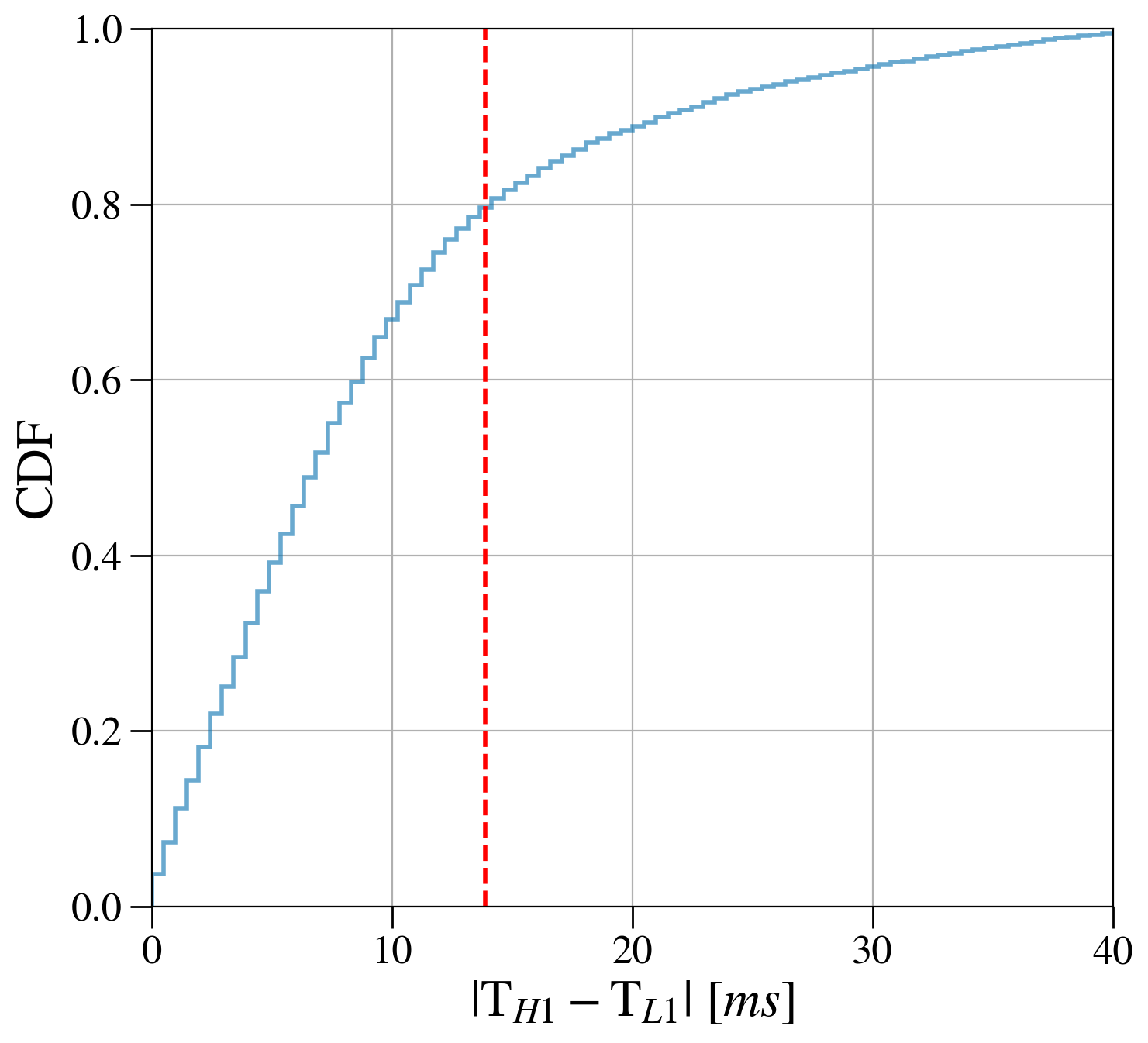
We compute the time delays by applying the trigger location algorithm to the simulated signals in the testing dataset. Fig. 11 shows the cumulative distribution of the measured time delays with a binning of ms. While physically, we expect the time delays to fall within ms duration owing to the maximum light travel time between the two LIGO detectors, it extends to ms for our dataset. Out of this, of the signals have a measured time delay ms. Those beyond this bound are largely due to incorrect trigger time estimation of low network SNR signals. Their estimated trigger time is compromised owing to poor contrast between the simulated signal and the Gaussian noise in the CWT maps. Thus, for time coincidence, we impose the criterion of ms for detection.


VI.4 Max-CWT Threshold

We observe that the SNR of the simulated signals and the corresponding maximum absolute CWT value max() follows a definite trend (see Fig. 12). Capitalizing on this information, we implement a Max-CWT Threshold to reject triggers with max() 120. The Max-CWT threshold is similar to the matched-filter SNR threshold often used in matched-filter searches. This constraint rejects approximately % of the total injections used, most with low optimal SNR. This also removes some of the noisy transients, thus improving our overall sensitivity.
VI.5 Efficacy of Thresholds
We compare the effectiveness of the time coincidence and Max-CWT thresholds by computing the distribution of the noise background in FAR vs rank space. For our purpose, we generate years of background data free of all coincident simulated signals and use it to estimate the FAR (see Eq. (7)). The results from our ablation study are shown in Fig. 13. A significant drop in FAR at low rank comes from the Max-CWT threshold. The time coincidence threshold reduces loud false alarms which are not coincident across the detectors. In THAMES we use both the time coincidence and Max-CWT thresholds.
VII Sensitivity Comparison with PyCBC-based searches
To assess the benefits of our newly developed search, we compare its performance against existing PyCBC-based modeled searches in overlapping target parameter space with the simulated signals. Later in this section, we also test the robustness of our search algorithm THAMES by testing it outside the target space.
VII.1 Detection Efficiency
We characterize the sensitivity of THAMES with the Receiver Operating Characteristics (ROC) curves. We compute the detection efficiency as the fraction of recovered simulated signals at a given FAR. We compare the sensitivity of THAMES with that of the PyCBC-IMBH and PyCBC-HM searches. The simulations used for this comparison are in the overlapping parameter space of mass ratio between these searches. The rest of the binary parameters of the simulated waveforms are similar to the ones in Table 1. These signals are isotropically distributed in sky location and uniformly in comoving volume with network optimal SNR in the range of 10-56.

Fig. 14 shows the result of our study. We find that THAMES outperforms the PyCBC-IMBH as well as the PyCBC-HM searches. At years and years, THAMES is 1.7 (1.22) and 2.66 (1.32) times more sensitive than PyCBC-IMBH (PyCBC-HM) respectively. This gain in detection efficiency is because THAMES is better equipped to detect signals and glitches than the other two searches, which allows it to discriminate glitches better. The improvement compared to PyCBC-IMBH is also because THAMES is trained on signals with higher harmonics as opposed to the latter, which uses the dominant harmonic of the binary as templates.
Since the only PyCBC-based search that overlaps with the training space of THAMES is PyCBC-Broad, we compare our search’s sensitivity against it. To do that, we use signals with but keep all the other parameters similar to the other comparison study. Fig. 14 summarizes the detection efficiency comparison results. We find that THAMES appreciably outperforms PyCBC-Broad search in this parameter space with an average sensitivity gain factor of 8.43 and 11.42 at IFAR = 100 years and IFAR = 1000 years, respectively, thus illustrating the capability of deep learning models to probe the complex signal morphology. The efficiency of PyCBC-Broad is low due to both look elsewhere effect and the omission of higher-order modes in the search templates.

In Fig. 15, we compare the detection efficiency as a function of the optimal coherent network SNR (Pai et al. 2001), at IFAR of 100 years. We observe that THAMES outperforms PyCBC-IMBH search at all values. However, as compared to the PyCBC-HM search, it outperforms only in mid-range values and performs comparably at high values of .
We also observe a progressive drop in the sensitivity of PyCBC-IMBH after achieving the peak sensitivity at of . This reduction in efficiency is due to an increased contribution from higher harmonics with increasing SNR, which PyCBC-IMBH search is not tuned to detect. However, the efficiency of PyCBC-HM search continues to increase with increasing SNR.
We observe a small decline in sensitivity of THAMES at high SNRs. A representative of these transients unveiled that model’s capacity to detect large SNR signals deteriorates slightly due to confusion with Koi Fishes and Extremely Loud glitch classes, especially at even higher SNRs. Here, the PyCBC-HM performs better than THAMES. Hence, a model trained on optimal SNR does not generalize to signals with higher optimal SNR, especially if the signal brings complex features with an increase in SNR. Further, the contrast between the signal transient and the background noise in a CWT map depends on the signal’s loudness, which is an inherent input to our machinery. We will investigate the latter in a future study.
VII.2 Sensitive Volume-Time Product

To compare the sensitivity of the four searches in the plane, we estimate the sensitive volume-time product (VTsen) using Monte-Carlo method (Usman et al. 2016). VTsen is the time and population-averaged spacetime volume to which the detector is sensitive at the chosen FAR threshold. The results from this analysis are summarized in Fig. 16. All the comparisons shown are carried out in the overlapping parameter set and using the same simulated signals discussed in Sec. VII.1.
The relative sensitivity of THAMES improves with an increase in detector frame total mass. This is due to THAMES’s better ability to discriminate glitches from binary signals, especially when the signal duration gets shorter with increasing detector frame total mass. The relatively poor VTsen at low detector frame total mass and low mass ratio (, ) is due to considerable confusion between loud (louder than the training set) IMBH binaries and blips. We observe that both matched-filter-based searches perform better than THAMES for and . THAMES improves over PyCBC-IMBH and PyCBC-HM by a factor of 5.24 and 2.92 respectively in range at an IFAR of 100 years. Further, THAMES outperforms PyCBC-Broad search at all detector frame total mass, with maximum gain in VTsen by a factor of for high detector frame total mass range.
Since a full analysis of the O3 (O3) run is beyond the scope of the current work, we approximate the statistical significance of a chosen set of O3a events. We summarize this in Appendix. C.
VIII Robustness Investigation
Typically the search algorithms are designed to target a subspace of the multi-dimensional signal parameter space. However, they are also tested outside their target space. Likewise, we perform two exercises to test the robustness of THAMES against various signals from asymmetric and binary systems. First, we consider signals from precessing binaries in the same parameter space. Second, we consider signals from binaries from all inclinations rather than only restricted to nearly edge-on binary orientations.
VIII.1 Susceptibility to Complex Morphology
Due to random pairing, hierarchically formed binaries are expected to have misalignment between the spins and the orbital angular momentum. Such a configuration induces relativistic precession effects, which causes the orbital plane to change its spatial orientation as the binary evolves. As a result, the emitted signal, depending on the binary’s orientation, can have a strong amplitude and phase modulation, which, in general, may not be sufficiently described by quasi-circular binary waveforms.
To check the detection efficiency of our search algorithm toward such generic sources, we simulated a population of quasi-spherical black hole binaries with mass, distance, binary orientation parameters, and optimal network SNRs similar to the ones used in Sec. VII.1. As for the spins, we sampled from a uniform distribution of spin magnitudes and isotropic distribution of spin orientations. Like before, we added the resulting set of simulated signals to the same representative section of Advanced LIGO detector data. We find that, at an IFAR of 100 years, our sensitive volume-time product drops from 0.52 Gpc3yr for non-precessing binaries to 0.30 Gpc3yr for precessing binaries, thus resulting in a 41.6% drop in sensitivity towards precessing sources as compared against a non-precessing binary population counterpart. This drop represents the inability of THAMES to capture the spin-precession signal morphology, which is distinct from the quasi-circular binary signals carrying only the higher-order modes. A detailed investigation on this is the topic for future work.
VIII.2 Generalization to All Inclination Angles
Most of the observed GW events are nearly optimally oriented since such sources are intrinsically loud and easier to detect. However, by construction, THAMES is designed to target almost edge-on sources with measurable higher-order mode content. We test our search’s capability to detect low-mass range binaries with binary parameters described in Table 1 but at an arbitrary inclination. The simulated sources have an isotropic distribution of inclinations between and , isotropic distribution over the sky sphere, and uniform distribution in comoving volume but with .
In Fig. 17, we observe an improvement in the model’s sensitivity to detect signals with inclinations beyond the training regime (black dashed lines). The recovered signals with IFAR above 100 years (and a rank greater than ) are distributed over all inclination angles (blue points). THAMES’s recovery outside the trained window is due to higher SNR and no additional morphological complexity in the signal.

However, we also observe that a small fraction of signals with high network optimal SNR are missed (red points), even for inclination angles in the training regime due to the similar reason explained in Sec. VII.1.
IX Conclusion
We describe the first end-to-end deep-learning-based modeled search, THAMES, to detect signals from mass asymmetric, nearly edge-on binaries. We use a deep learning model with Inception-v3 network architecture to classify the CWT maps of data from the interferometers into signals from non-optimally oriented mass asymmetric binaries and a variety of noisy glitches which resemble binary signals. We devise a novel quadrature-sum detection statistic based on the evidence provided by the deep learning model to rank all the simulated signals and background triggers. The primary rationale behind the construction is that the transients with inconsistent morphology with the trained signals are heavily penalized, and coincident signals with nearly equiprobability in both the LIGO detectors are rewarded. We utilize the time-coincidence condition and Max-CWT threshold to suppress the false alarms in terms of the noisy glitches.
The detection efficiency of our search is significantly greater than those of other modeled searches with overlapping parameter space. In fact, we find that our search is a factor of 5.24 () more sensitive than that of the PyCBC-IMBH (PyCBC-Broad) search at an IFAR = 100 years for systems with total mass in the range 400-500 . These matched-filter searches are primarily penalized due to the usage of templates without higher-order harmonics. Therefore, this demonstrates the capability of deep learning techniques to effectively probe complex signal morphologies inherent in signals from asymmetric, edge-on binary that carry higher-order modes. We also compared our search performance against that of the recently developed PyCBC-HM search and found that depending on the system’s total mass, the gain in sensitive volume-time is at most by a factor of 2.92. This clearly illustrates deep learning techniques’ better signal-noise discrimination power, especially for short-duration signals. However, we report that our search slightly underperforms for binaries with a low detector frame total mass of 100-200 . This is due to significant confusion with blips in this parameter space. Furthermore, THAMES is limited by its susceptibility to complex and loud signal morphology, which it is not trained on. Despite such limitations, deep learning techniques are up-and-coming due to their ability to leverage the morphology of glitches to better separate transient noises from signals and the ease of expanding to any search space.
We need to undergo a couple of upgrades to take advantage of the benefits offered by our deep-learning-based detection algorithm. There is a scope for improvement in our time estimation technique which currently misestimates the time for low SNR signals. At present, the least count of the image is five times the sampling interval of our data ( ms), which affects our trigger time estimation accuracy. Since the time-coincidence threshold is the root cause for the principle improvement in background trigger distribution, possibly an improvement in the time estimation technique will further improve the detection efficiency. Secondly, the current search uses continuous wavelet transform to generate spectrograms, which is time-consuming. More time-efficient approaches need to be explored.
Encouraged by the remarkable sensitivity of THAMES in detecting binary signals with higher-order modes, we look forward to extending this search to precessing and eccentric waveforms that carry additional signal complexity. We also plan on extending the search to a multi-detector network.

Acknowledgements.
We thank Ik Siong Heng and Juan Calderón Bustillo for comments on the manuscript. This research has made use of data, software, and/or web tools obtained from the Gravitational Wave Open Science Center (https://www.gw-openscience.org), a service of LIGO Laboratory, the LIGO Scientific Collaboration and the Virgo Collaboration. Virgo is funded by the French Centre National de Recherche Scientifique (CNRS), the Italian Istituto Nazionale della Fisica Nucleare (INFN), and the Dutch Nikhef, with contributions by Polish and Hungarian institutes. This material is based upon work supported by NSF’s LIGO Laboratory, which is a major facility fully funded by the National Science Foundation. The authors are grateful for computational resources provided by the LIGO Laboratory and supported by National Science Foundation Grants PHY0757058 and PHY-0823459. The authors thank the G-Suite products and Google Colaboratory for providing the powerful hardware option of GPU (https://colab.research.google.com/). KC acknowledges the MHRD, the Government of India, for the fellowship support. AP acknowledges the support from SERB-Power-fellowship grant SPF/2021/000036, DST, India. This document has LIGO DCC No LIGO-P2200227.Appendix A Network Architecture
The network proposed in THAMES uses transfer learning by reusing the Inception-v3 pre-trained model (Szegedy et al. 2015a; Szegedy et al. 2014). The key idea behind inception modules is to formulate convolution operations optimally to capture salient parts of an image. Smaller convolution kernels are optimal for capturing local features (with low size variations). Similarly, larger kernels are preferred to capture global features (with high size variations). To cater to this need, the use of multiple stacked convolution operations will make the network too deep, thus causing over-fitting and a tremendous increase in training time (Ying 2019; Salman and Liu 2019). Inception modules tackle these problems by having wider networks with various convolution sizes and max-pooling operations to downscale the image appropriately (Gholamalinezhad and Khosravi 2020). These max-pooling layers also have the added advantage of adding translation, rotation, and scale invariance to the deep learning model. Therefore, the construct of a Naive Inception Module will have various convolutional kernels (, , ) and a max-pooling filter (), the output from which will be concatenated and fed into the next layer (see top-left panel of Fig. 18). Since the time complexity of an convolution operation is , this construct of the naive inception module increases the computational cost. The developers of inception modules tackle this problem by adding convolutions before the and convolutions and after the max-pooling layer to reduce the number of input channels and hence, the computational cost. This construct is called Inception Module with Dimension Reductions. Despite this, the overall network is very deep, leading to a problem of vanishing gradients. This limitation is lifted by adding Auxiliary Classifiers so that the network takes into account an “auxiliary loss”, in addition to the training loss when learning (Szegedy et al. 2015b; Lee et al. 2015).
The computational cost of larger convolutions can be further reduced by factorizing them into two smaller convolution operations, such that the receptive fields of the two operations remains the same (Szegedy et al. 2015a). This way, a convolution can be factorized into two convolutions, thus reducing the computational complexity by , while retaining the same receptive field. We refer to the module with these amendments as Inception Module A. Similarly, we further modify this module by factorizing convolutions into and convolutions, thus reducing the computational complexity by which we refer as Inception Module B. The loss of information due to a stack of convolutions which significantly reduces the image’s dimensions can be fixed by expanding the filters. This we refer to as Inception Module C.
| Event Name | GPS Time [s] | [] | IFAR [yr] | |||||
|---|---|---|---|---|---|---|---|---|
| THAMES | PyCBC-IMBH | PyCBC-HM | GWTC-2 | IAS | ||||
| 55.5 | 1.34 | 47.52 | 62.66 | 60.60 | ||||
| 44.2 | 3.63 | 38.88 | - | 10.50 | ||||
| 315.4 | 1.39 | 2.12 | - | - | ||||
| 73.8 | 1.98 | 47.52 | - | 1.49 | ||||
| 154.2 | 1.65 | 4.95 | 31.35 | |||||
| 278.2 | 1.28 | 11.46 | 726.65 | - | ||||
| 92.6 | 1.27 | 4.94 | ||||||
| 172.2 | 1.62 | 915.02 | 2.07 | |||||
| 144.0 | 3.35 | 17.11 | - | - | ||||
Our detailed network architecture is represented in Fig. 18. Our deep learning network comprises three inception modules A, five inception modules B, and two inception modules C. The size of our CWT maps are 135 pixels 735 pixels 3 channels, which are fed into input convolutional layers, followed by inception modules with interleaved grid size reduction layers. As discussed above, an auxiliary classifier is used to avoid the vanishing gradients problem. All these layers are initialized with pre-trained weights and are only fine-tuned during training to extract generic features from our dataset. The features extracted from the input by our convolutional base have a size of .

These feature maps are then fed into a set of prediction layers, which are randomly initialized for training. Our first filter in this set of prediction layers is an average-pooling layer (Lin et al. 2013). Since the entire Inception-v3 network only uses max-pooling layers, which only retain the feature map’s most prominent (bright) attributes, we choose to use an average pooling layer in the end to get smooth features. Next, we use a densely connected layer since it passes information from each neuron in the previous layer to each neuron in the following layer, thus increasing each neuron’s receptive field to take into account features from the entire image before making any prediction (Huang et al. 2016). We also use a drop-out layer to avoid overfitting when using densely connected layers (Srivastava et al. 2014). Finally, we use a dense connected layer with softmax (Goodfellow et al. 2016) activation function to output the relative probability of a CWT map to belong to one of the nine trained classes.
Appendix B Detection Statistic Comparison
Here, we compare the benefits of the quadrature sum statistic defined in Eq. (12) with the conventionally used rank defined as the joint probability statistic under the assumption of uncorrelated noise between H1 and L1 as:
| (13) |
with , being the probability of the data containing an binary signal in H1 and L1, respectively. To understand their impact on search sensitivity, we, in Fig. 19, compare the detection efficiency of THAMES using these two different ranking statistics. We see that the quadrature sum statistic () performs better than the joint probability statistic (), reconfirming the ability of to separate the signal and noise transients, also shown in Fig. 9.
Appendix C Surrogate Open-Box Results
Though doing a full analysis of the O3 data of Advanced LIGO detectors is beyond the scope of the current work, we wish to get an estimate of what we should expect from the extended analysis. We, therefore, assume that the estimated background trigger distribution remains more or less the same during the duration of the first part of the O3 run. We use this to estimate the IFAR of a chosen set of statistically significant candidates already reported elsewhere (Abbott et al. 2021a; Olsen et al. 2022). Table 2 lists the events which are recovered by THAMES with IFAR year. We note that the (expected) reduced statistical significance of the reported events for those obtained by existing searches highlights that these candidates are outside our target parameter space.
References
- Abbott et al. (2019) B. P. Abbott et al. (LIGO Scientific, Virgo), Phys. Rev. X 9, 031040 (2019), arXiv:1811.12907 [astro-ph.HE] .
- Nitz et al. (2019) A. H. Nitz, C. Capano, A. B. Nielsen, S. Reyes, R. White, D. A. Brown, and B. Krishnan, Astrophys. J. 872, 195 (2019), arXiv:1811.01921 [gr-qc] .
- Venumadhav et al. (2020) T. Venumadhav, B. Zackay, J. Roulet, L. Dai, and M. Zaldarriaga, Phys. Rev. D 101, 083030 (2020), arXiv:1904.07214 [astro-ph.HE] .
- Zackay et al. (2021) B. Zackay, L. Dai, T. Venumadhav, J. Roulet, and M. Zaldarriaga, Phys. Rev. D 104, 063030 (2021), arXiv:1910.09528 [astro-ph.HE] .
- Zackay et al. (2019) B. Zackay, T. Venumadhav, L. Dai, J. Roulet, and M. Zaldarriaga, Phys. Rev. D 100, 023007 (2019), arXiv:1902.10331 [astro-ph.HE] .
- Nitz et al. (2020) A. H. Nitz, T. Dent, G. S. Davies, S. Kumar, C. D. Capano, I. Harry, S. Mozzon, L. Nuttall, A. Lundgren, and M. Tápai, Astrophys. J. 891, 123 (2020), arXiv:1910.05331 [astro-ph.HE] .
- Abbott et al. (2021a) R. Abbott et al. (LIGO Scientific, Virgo), Phys. Rev. X 11, 021053 (2021a), arXiv:2010.14527 [gr-qc] .
- Abbott et al. (2021b) R. Abbott et al. (LIGO Scientific, VIRGO, KAGRA), (2021b), arXiv:2111.03606 [gr-qc] .
- Nitz et al. (2021a) A. H. Nitz, C. D. Capano, S. Kumar, Y.-F. Wang, S. Kastha, M. Schäfer, R. Dhurkunde, and M. Cabero, Astrophys. J. 922, 76 (2021a), arXiv:2105.09151 [astro-ph.HE] .
- Nitz et al. (2021b) A. H. Nitz, S. Kumar, Y.-F. Wang, S. Kastha, S. Wu, M. Schäfer, R. Dhurkunde, and C. D. Capano, (2021b), arXiv:2112.06878 [astro-ph.HE] .
- Olsen et al. (2022) S. Olsen, T. Venumadhav, J. Mushkin, J. Roulet, B. Zackay, and M. Zaldarriaga, (2022), arXiv:2201.02252 [astro-ph.HE] .
- Abbott et al. (2020a) R. Abbott et al. (LIGO Scientific, Virgo), Phys. Rev. Lett. 125, 101102 (2020a), arXiv:2009.01075 [gr-qc] .
- Abbott et al. (2020b) R. Abbott et al. (LIGO Scientific, Virgo), Astrophys. J. Lett. 900, L13 (2020b), arXiv:2009.01190 [astro-ph.HE] .
- Szczepańczyk et al. (2021) M. Szczepańczyk et al., Phys. Rev. D 103, 082002 (2021), arXiv:2009.11336 [astro-ph.HE] .
- Woosley and Heger (2021) S. E. Woosley and A. Heger, Astrophys. J. Lett. 912, L31 (2021), arXiv:2103.07933 [astro-ph.SR] .
- Gerosa et al. (2021) D. Gerosa, N. Giacobbo, and A. Vecchio, Astrophys. J. 915, 56 (2021), arXiv:2104.11247 [astro-ph.HE] .
- Baibhav et al. (2020) V. Baibhav, D. Gerosa, E. Berti, K. W. K. Wong, T. Helfer, and M. Mould, Phys. Rev. D 102, 043002 (2020), arXiv:2004.00650 [astro-ph.HE] .
- Berti et al. (2007) E. Berti, V. Cardoso, J. A. Gonzalez, U. Sperhake, M. Hannam, S. Husa, and B. Bruegmann, Phys. Rev. D 76, 064034 (2007), arXiv:gr-qc/0703053 .
- Mills and Fairhurst (2021) C. Mills and S. Fairhurst, Phys. Rev. D 103, 024042 (2021), arXiv:2007.04313 [gr-qc] .
- Calderón Bustillo et al. (2016) J. Calderón Bustillo, S. Husa, A. M. Sintes, and M. Pürrer, Phys. Rev. D 93, 084019 (2016), arXiv:1511.02060 [gr-qc] .
- Calderón Bustillo et al. (2017) J. Calderón Bustillo, P. Laguna, and D. Shoemaker, Phys. Rev. D 95, 104038 (2017), arXiv:1612.02340 [gr-qc] .
- Varma et al. (2014) V. Varma, P. Ajith, S. Husa, J. C. Bustillo, M. Hannam, and M. Pürrer, Phys. Rev. D 90, 124004 (2014), arXiv:1409.2349 [gr-qc] .
- Usman et al. (2019) S. A. Usman, J. C. Mills, and S. Fairhurst, Astrophys. J. 877, 82 (2019), arXiv:1809.10727 [gr-qc] .
- Vitale and Chen (2018) S. Vitale and H.-Y. Chen, Phys. Rev. Lett. 121, 021303 (2018), arXiv:1804.07337 [astro-ph.CO] .
- Carullo et al. (2019) G. Carullo, W. Del Pozzo, and J. Veitch, Phys. Rev. D 99, 123029 (2019), [Erratum: Phys.Rev.D 100, 089903 (2019)], arXiv:1902.07527 [gr-qc] .
- Isi et al. (2019) M. Isi, M. Giesler, W. M. Farr, M. A. Scheel, and S. A. Teukolsky, Phys. Rev. Lett. 123, 111102 (2019), arXiv:1905.00869 [gr-qc] .
- Bustillo et al. (2021) J. C. Bustillo, P. D. Lasky, and E. Thrane, Phys. Rev. D 103, 024041 (2021), arXiv:2010.01857 [gr-qc] .
- Varma et al. (2020) V. Varma, M. Isi, and S. Biscoveanu, Phys. Rev. Lett. 124, 101104 (2020), arXiv:2002.00296 [gr-qc] .
- Calderón Bustillo et al. (2018a) J. Calderón Bustillo, J. A. Clark, P. Laguna, and D. Shoemaker, Phys. Rev. Lett. 121, 191102 (2018a), arXiv:1806.11160 [gr-qc] .
- Calderón Bustillo et al. (2018b) J. Calderón Bustillo, F. Salemi, T. Dal Canton, and K. P. Jani, Phys. Rev. D 97, 024016 (2018b), arXiv:1711.02009 [gr-qc] .
- Chandra et al. (2022) K. Chandra, J. Calderón Bustillo, A. Pai, and I. Harry, (2022), arXiv:2207.01654 [gr-qc] .
- Chandra et al. (2021) K. Chandra, V. Villa-Ortega, T. Dent, C. McIsaac, A. Pai, I. W. Harry, G. S. C. Davies, and K. Soni, Phys. Rev. D 104, 042004 (2021), arXiv:2106.00193 [gr-qc] .
- Abbott et al. (2018) B. P. Abbott et al. (LIGO Scientific, Virgo), Class. Quant. Grav. 35, 065010 (2018), arXiv:1710.02185 [gr-qc] .
- Allen (2005) B. Allen, Phys. Rev. D 71, 062001 (2005), arXiv:gr-qc/0405045 .
- Usman et al. (2016) S. A. Usman et al., Class. Quant. Grav. 33, 215004 (2016), arXiv:1508.02357 [gr-qc] .
- Cuoco et al. (2021) E. Cuoco et al., Mach. Learn. Sci. Tech. 2, 011002 (2021), arXiv:2005.03745 [astro-ph.HE] .
- Aasi et al. (2015) J. Aasi et al. (LIGO Scientific), Class. Quant. Grav. 32, 074001 (2015), arXiv:1411.4547 [gr-qc] .
- Flandrin (2018) P. Flandrin, Explorations in Time-Frequency Analysis (Cambridge University Press, 2018).
- Szegedy et al. (2014) C. Szegedy et al., “Going deeper with convolutions,” (2014), arXiv:1409.4842 [cs.CV] .
- Szegedy et al. (2015a) C. Szegedy et al., “Rethinking the inception architecture for computer vision,” (2015a), arXiv:1512.00567 [cs.CV] .
- Blanchet (2014) L. Blanchet, Living Rev. Rel. 17, 2 (2014), arXiv:1310.1528 [gr-qc] .
- Cotesta et al. (2018) R. Cotesta, A. Buonanno, A. Bohé, A. Taracchini, I. Hinder, and S. Ossokine, Phys. Rev. D 98, 084028 (2018), arXiv:1803.10701 [gr-qc] .
- Sathyaprakash and Dhurandhar (1991) B. S. Sathyaprakash and S. V. Dhurandhar, Phys. Rev. D 44, 3819 (1991).
- Klimenko et al. (2016) S. Klimenko et al., Phys. Rev. D 93, 042004 (2016), arXiv:1511.05999 [gr-qc] .
- Babak et al. (2013) S. Babak et al., Phys. Rev. D 87, 024033 (2013), arXiv:1208.3491 [gr-qc] .
- Nitz et al. (2017) A. H. Nitz, T. Dent, T. Dal Canton, S. Fairhurst, and D. A. Brown, Astrophys. J. 849, 118 (2017), arXiv:1705.01513 [gr-qc] .
- Nitz (2018) A. H. Nitz, Class. Quant. Grav. 35, 035016 (2018), arXiv:1709.08974 [gr-qc] .
- Cornish et al. (2021) N. J. Cornish, T. B. Littenberg, B. Bécsy, K. Chatziioannou, J. A. Clark, S. Ghonge, and M. Millhouse, Phys. Rev. D 103, 044006 (2021), arXiv:2011.09494 [gr-qc] .
- Arai and Kapoor (2020) K. Arai and S. Kapoor, eds., Advances in Computer Vision (Springer International Publishing, 2020).
- Mahabal et al. (2019) A. Mahabal et al., Publications of the Astronomical Society of the Pacific 131, 038002 (2019).
- Sanchez Saez (2022) P. Sanchez Saez, in SciOps 2022: Artificial Intelligence for Science and Operations in Astronomy (SCIOPS). Proceedings of the ESA/ESO SCOPS Workshop held 16-20 May (2022) p. 17.
- Vibho and Assaf (2022) A. Vibho and R. Assaf, Astron. Comput. 39, 100566 (2022).
- Barchi et al. (2020) P. H. Barchi, R. R. de Carvalho, R. R. Rosa, R. A. Sautter, M. Soares-Santos, B. A. D. Marques, E. Clua, T. S. Gonçalves, C. de Sá-Freitas, and T. C. Moura, Astron. Comput. 30, 100334 (2020), arXiv:1901.07047 [astro-ph.IM] .
- González et al. (2018) R. González, R. Muñoz, and C. Hernández, Astronomy and Computing 25, 103 (2018).
- Duev et al. (2019) D. A. Duev et al., Monthly Notices of the Royal Astronomical Society 486, 4158 (2019).
- George and Huerta (2017) D. George and E. A. Huerta, in NiPS Summer School 2017 (2017) arXiv:1711.07966 [gr-qc] .
- Gabbard et al. (2018) H. Gabbard, M. Williams, F. Hayes, and C. Messenger, Phys. Rev. Lett. 120, 141103 (2018), arXiv:1712.06041 [astro-ph.IM] .
- Álvares et al. (2020) J. a. D. Álvares et al. (2020) arXiv:2011.10425 [gr-qc] .
- Chatterjee et al. (2021) C. Chatterjee, L. Wen, F. Diakogiannis, and K. Vinsen, Phys. Rev. D 104, 064046 (2021), arXiv:2105.03073 [gr-qc] .
- Gebhard et al. (2019) T. D. Gebhard, N. Kilbertus, I. Harry, and B. Schölkopf, Phys. Rev. D 100, 063015 (2019).
- Schäfer et al. (2022) M. B. Schäfer, O. Zelenka, A. H. Nitz, F. Ohme, and B. Brügmann, Phys. Rev. D 105, 043002 (2022), arXiv:2106.03741 [astro-ph.IM] .
- Schäfer and Nitz (2022) M. B. Schäfer and A. H. Nitz, Phys. Rev. D 105, 043003 (2022).
- López et al. (2021) M. López, M. Drago, I. D. Palma, F. Ricci, and P. Cerdá-Durán, in International Conference on Content-Based Multimedia Indexing (2021).
- George et al. (2018) D. George, H. Shen, and E. A. Huerta, Phys. Rev. D 97, 101501 (2018).
- Lopez et al. (2022) D. Lopez, V. Gayathri, A. Pai, I. S. Heng, C. Messenger, and S. K. Gupta, Phys. Rev. D 105, 063024 (2022), arXiv:2112.06608 [gr-qc] .
- Zevin et al. (2017) M. Zevin et al., Class. Quant. Grav. 34, 064003 (2017), arXiv:1611.04596 [gr-qc] .
- Cabero et al. (2019) M. Cabero et al., Class. Quant. Grav. 36, 15 (2019), arXiv:1901.05093 [physics.ins-det] .
- Davis (2019) D. Davis, Improving the Sensitivity of Advanced Ligo Through Detector Characterization, Ph.D. thesis, Syracuse U., Syracuse U. (2019).
- Soni et al. (2021) S. Soni et al., Class. Quant. Grav. 38, 195016 (2021), arXiv:2103.12104 [gr-qc] .
- Davis et al. (2021) D. Davis et al. (LIGO), Class. Quant. Grav. 38, 135014 (2021), arXiv:2101.11673 [astro-ph.IM] .
- Abbott et al. (2016) B. P. Abbott et al. (LIGO Scientific, Virgo), Class. Quant. Grav. 33, 134001 (2016), arXiv:1602.03844 [gr-qc] .
- Nuttall et al. (2015) L. Nuttall et al., Class. Quant. Grav. 32, 245005 (2015), arXiv:1508.07316 [gr-qc] .
- Santamaria et al. (2010) L. Santamaria et al., Phys. Rev. D 82, 064016 (2010), arXiv:1005.3306 [gr-qc] .
- Campanelli et al. (2006) M. Campanelli, C. O. Lousto, and Y. Zlochower, Phys. Rev. D 74, 041501 (2006), arXiv:gr-qc/0604012 .
- Abbott et al. (2022) R. Abbott et al. (LIGO Scientific, VIRGO, KAGRA), Astron. Astrophys. 659, A84 (2022), arXiv:2105.15120 [astro-ph.HE] .
- Pratt (1992) L. Y. Pratt, in Advances in Neural Information Processing Systems, Vol. 5, edited by S. Hanson, J. Cowan, and C. Giles (Morgan-Kaufmann, 1992).
- Zhuang et al. (2019) F. Zhuang, Z. Qi, K. Duan, D. Xi, Y. Zhu, H. Zhu, H. Xiong, and Q. He, “A comprehensive survey on transfer learning,” (2019).
- Ribani and Marengoni (2019) R. Ribani and M. Marengoni, in 2019 32nd SIBGRAPI Conference on Graphics, Patterns and Images Tutorials (SIBGRAPI-T) (2019) pp. 47–57.
- Yang et al. (2022) S. Yang, W. Xiao, M. Zhang, S. Guo, J. Zhao, and F. Shen, “Image data augmentation for deep learning: A survey,” (2022).
- Vakili et al. (2020) M. Vakili, M. Ghamsari, and M. Rezaei, “Performance analysis and comparison of machine and deep learning algorithms for iot data classification,” (2020).
- Goodfellow et al. (2016) I. Goodfellow, Y. Bengio, and A. Courville, Deep Learning (MIT Press, 2016) http://www.deeplearningbook.org.
- Abadi et al. (2016) M. Abadi et al., (2016), arXiv:1603.04467 [cs.DC] .
- Bisong (2019) E. Bisong, “Google colaboratory,” in Building Machine Learning and Deep Learning Models on Google Cloud Platform: A Comprehensive Guide for Beginners (Apress, Berkeley, CA, 2019) pp. 59–64.
- Boldaji and Semnani (2021) M. N. Boldaji and S. H. Semnani, “Color image segmentation using multi-objective swarm optimizer and multi-level histogram thresholding,” (2021).
- Pai et al. (2001) A. Pai, S. Dhurandhar, and S. Bose, Phys. Rev. D 64, 042004 (2001), arXiv:gr-qc/0009078 .
- Ying (2019) X. Ying, Journal of Physics: Conference Series 1168, 022022 (2019).
- Salman and Liu (2019) S. Salman and X. Liu, “Overfitting mechanism and avoidance in deep neural networks,” (2019).
- Gholamalinezhad and Khosravi (2020) H. Gholamalinezhad and H. Khosravi, “Pooling methods in deep neural networks, a review,” (2020).
- Szegedy et al. (2015b) C. Szegedy et al., in 2015 IEEE Conference on Computer Vision and Pattern Recognition (CVPR) (2015) pp. 1–9.
- Lee et al. (2015) C.-Y. Lee, S. Xie, P. Gallagher, Z. Zhang, and Z. Tu, in Proceedings of the Eighteenth International Conference on Artificial Intelligence and Statistics, Proceedings of Machine Learning Research, Vol. 38, edited by G. Lebanon and S. V. N. Vishwanathan (PMLR, San Diego, California, USA, 2015) pp. 562–570.
- Lin et al. (2013) M. Lin, Q. Chen, and S. Yan, “Network in network,” (2013).
- Huang et al. (2016) G. Huang, Z. Liu, L. van der Maaten, and K. Q. Weinberger, “Densely connected convolutional networks,” (2016).
- Srivastava et al. (2014) N. Srivastava, G. Hinton, A. Krizhevsky, I. Sutskever, and R. Salakhutdinov, Journal of Machine Learning Research 15, 1929 (2014).