Towards Generating Large Synthetic Phytoplankton Datasets
for Efficient Monitoring of Harmful Algal Blooms

Nitpreet Bamra Affiliation: University of Waterloo, Vikram Voleti Affiliation: Blue Lion Labs, Affiliation: Mila, University of Montreal{nbamra, jdeglint}@uwaterloo.ca Alexander Wong Affiliation: University of Waterloo, Affiliation: Blue Lion Labs, Jason Deglint Affiliation: University of Waterloo, Affiliation: Blue Lion Labs,

Abstract

Climate change is increasing the frequency and severity of harmful algal blooms (HABs), which cause significant fish deaths in aquaculture farms. This contributes to ocean pollution and greenhouse gas (GHG) emissions since dead fish are either dumped into the ocean or taken to landfills, which in turn negatively impacts the climate. Currently, the standard method to enumerate harmful algae and other phytoplankton is to manually observe and count them under a microscope. This is a time-consuming, tedious and error-prone process, resulting in compromised management decisions by farmers. Hence, automating this process for quick and accurate HAB monitoring is extremely helpful. However, this requires large and diverse datasets of phytoplankton images, and such datasets are hard to produce quickly. In this work, we explore the feasibility of generating novel high-resolution photorealistic synthetic phytoplankton images, containing multiple species in the same image, given a small dataset of real images. To this end, we employ Generative Adversarial Networks (GANs) to generate synthetic images. We evaluate three different GAN architectures: ProjectedGAN, FastGAN, and StyleGANv2 using standard image quality metrics. We empirically show the generation of high-fidelity synthetic phytoplankton images using a training dataset of only 961 real images. Thus, this work demonstrates the ability of GANs to create large synthetic datasets of phytoplankton from small training datasets, accomplishing a key step towards sustainable systematic monitoring of harmful algal blooms.

Introduction

When different phytoplankton and algae species grow uncontrollably, they can form harmful algal blooms (HABs). These HABs can produce lethal toxins and hypoxic “dead” zones, causing catastrophic impacts on various industries such as aquaculture and real estate [\citeauthoryearBrooks et al.2016], as well as negatively impacting wildlife and the environment [\citeauthoryearGranéli and Turner2006]. Further, research shows that climate change is increasing the frequency and severity of these HABs [\citeauthoryearWells et al.2020]. For example, in 2016, a HAB outbreak in Chile killed over 27 million farmed trout and salmon [\citeauthoryearMontes et al.2018]. Furthermore, from 2015-2019, farmed salmon deaths due to fatal diseases caused by HABs increased by 27.8% from 41.3 to 52.8 million [\citeauthoryearPersson et al.2022]. When millions of fish die due to HABs and other diseases, they are disposed of by being dumped back into the ocean, causing ocean pollution, or being brought to landfills, causing increased greenhouse gas (GHG) emissions [\citeauthoryearArmijo et al.2020, \citeauthoryearBustos, Ramírez, and Rudolf2021]. Furthermore, as GHG emissions increase, the surface temperature and acidity of water bodies increase simultaneously, creating an ideal environment for HABs to grow, thereby leading to an endless cycle of increasing GHG emissions [\citeauthoryearMoore et al.2008].

A promising solution to mitigate this problem is quicker and more consistent monitoring of HABs. This would improve farm yields, as well as reduce ocean pollution and GHG emissions. However, rapid identification is challenging due to the extremely time-consuming, tedious and error-prone process for a taxonomist to manually analyze and classify these algae species [\citeauthoryearMcQuatters-Gollop et al.2017].

Given digital microscopy and novel deep learning methods, it is possible to improve both the speed and accuracy of current algae detection methods [\citeauthoryearSalido et al.2020]. However, such methods require the collection of large and diverse phytoplankton datasets, which is both expensive and tedious, thereby limiting the effectiveness of current HAB monitoring as shown in the “Current Method” section of Figure 4. Moreover, it is important that such datasets match real images as far as possible, so they should ideally include multiple phytoplankton species in the same image.

In this work, we propose a framework to generate high-fidelity and diverse synthetic datasets of phytoplankton, motivated by the potential to expedite, improve, and standardize algae and phytoplankton detection. This is shown in the “Proposed Method” section of Figure 4. We utilize Generative Adversarial Networks (GANs) to generate novel synthetic images, but in principle any image generation technique could be used. Our main contributions in this work are: (1) we explore three state-of-the-art (SOTA) GAN architectures for generating synthetic datasets of image samples containing multiple phytoplankton species, (2) we evaluate the generated images using standard image quality metrics, and (3) we validate the novelty of generated images by checking for memorization of the training images.

Refer to caption — Figure 1: The current (top) and proposed (bottom) deep learning algae detection methods. Our proposed framework leads to improved HAB monitoring, the initial step being the generation of a large and synthetic algae dataset.

Related Works

GANs are some of the most effective machine learning frameworks for generating synthetic outputs from random noise inputs [\citeauthoryearGoodfellow et al.2014]. A GAN model contains two sub-models: a generator $G$ and a discriminator $D$ . The generator works to create realistic synthetic images from a random noise input, and the discriminator deciphers whether an image is real or generated. To improve the quality of the generated images, the two sub-models compete against each other in a two-player min-max game, the objective is calculated using Equation 1:

\mathop{min}_{{G}}\mathop{max}_{{D}}(E_{x}[\log D(x)]+E_{z}[log(1-D(G(z)))])

(1)

In Equation 1, $D(x)$ and $D(G(z))$ denote the probability that an instance of real data $x$ or generated images $G(z)$ from noise instance $z$ is from the real dataset or the generator. $E_{x}$ and $E_{z}$ denote the expected values from all real data inputs to the discriminator and random noise inputs to the generator, respectively.

A study published in 2017 [\citeauthoryearWang et al.2017] suggested that convolutional neural networks tend to be biased towards larger specimen classes. It then proposed to use the ConditionalGAN model [\citeauthoryearMirza and Osindero2014] to generate synthetic images of plankton species to address the hardships of species generation given few per-class examples.

Another study published in 2021 [\citeauthoryearLi et al.2021] explores the use of the CycleGAN model [\citeauthoryearZhu et al.2017] to address the imbalance within the classes of plankton species by generating more of the low-class species. The CycleGAN architecture allows for image-to-image translation by learning and interchanging the mapping features of the two images.

Lastly, a 2022 study from Inje University [\citeauthoryearAbdullah et al.2022] focused on using the DCGAN model [\citeauthoryearRadford, Metz, and Chintala2016] to generate microscopic images of phytoplankton to enhance the size of their dataset. The DCGAN model is an extension of the original GAN model, the main difference being the use of deep convolutional neural networks for both the discriminator and generator, instead of fully connected layers. This study used a dataset of 400 single-organism microscopic images of 4 different algae species. They fed these 400 images to the DCGAN, using it as an “advanced augmentation” tool to successfully double their dataset.

In contrast, our investigation focuses on generating a novel high-quality synthetic dataset of 11 organism types, in which each image contains multiple algae species. Furthermore, we explore three different SOTA GAN architectures, and generate high-resolution images.

Methodology

GAN Architectures

Three GAN models that have proven to produce high-fidelity synthetic images consistently are ProjectedGAN [\citeauthoryearSauer et al.2021], FastGAN [\citeauthoryearLiu et al.2021], and StyleGANv2 [\citeauthoryearKarras et al.2019].

Projected GAN. The ProjectedGAN [\citeauthoryearSauer et al.2021] works by projecting features from both generated and real images into a pre-trained feature space instead of the standard input space. The min-max equation of ProjectedGAN differs from that of vanilla GAN by introducing projections of different feature vectors $P_{\iota}(x)$ into the discriminator’s original input space, and is calculated using Equation 2:

\mathop{min}_{{G}}\mathop{max}_{{D_{\iota}}}\Sigma_{\iota\epsilon\zeta}(E_{x}[\log D_{\iota}(P_{\iota}(x))]\\ +E_{z}[log(1-D_{\iota}(P_{\iota}(G(z))))])

(2)

In Equation 2, $D_{\iota}$ denotes a set of independent discriminators which operate on distinct projected features and $\Sigma_{\iota\epsilon\zeta}$ denotes the summation of all components in the equation.

FastGAN. The FastGAN [\citeauthoryearLiu et al.2021] model reduces the significant computational needs and the large number of training images required for a GAN to train, by incorporating a Skip-Layer channel-wise Excitation (SLE) module. The SLE module is calculated using Equation 3, where $y$ is the output feature map of the SLE model, $W_{i}$ is the weight which needs to be learned by the model, and $x_{low}$ / $x_{high}$ represent the low/high resolution feature maps, respectively.

y=F(x_{low},(W_{i}))*x_{high}\vskip-8.53581pt

(3)

StyleGANv2. StyleGANv2 [\citeauthoryearKarras et al.2019] is one of the SOTA GAN models that consistently produces high-fidelity synthetic images without using pre-trained feature spaces. This is achieved by first transforming the input noise vector into an “ intermediate latent code” using a mapping network. These intermediate codes represent multiple distinct “styles”, which allows for the GAN to generate images with multiple layers of details, ranging from course details like algae shape and orientation, to fine details like algae flagella and cilia. These “styles” are then processed through an adaptive instance normalization (AdaIN) process, as explained in Equation 4:

AdaIN(x_{i},y)=y_{s,i}\frac{x_{i}-\mu(x_{i})}{\sigma(x_{i})}+y_{b,i}

(4)

In Equation 4, $x_{i}$ represents a feature map, $y_{b}$ and $y_{s}$ represent corresponding scalar component from the respective style and $\mu$ / $\sigma$ represent scalable factors for input normalization [\citeauthoryearHuang and Belongie2017].

Table 1: Image quality and computational metrics from each GAN model. The SytleGANv2 consistently yields the lowest FID and KID scores (see bold values) supporting that the SytleGANv2 generated the best synthetic images.

GAN Model	Data Size	Resolution	Iterations	Batch Size	Training Time	FID	KID	GPU model
ProjectedGAN	1922	256x256	1,427,400	64	04d 00h 45m	113.107	0.050	GTX TITAN X
ProjectedGAN	1922	256x256	1,008,000	64	02d 20h 33m	226.317	0.093	GTX TITAN X
FastGAN	961	1024x1024	50,000	8	21h 33m	186.690	0.163	GTX TITAN X
	9610	1024x1024	25,000	8	10h 46m	130.201	0.090	GTX TITAN X
	9610	1024x1024	50,000	8	16h 00m	166.062	0.083	GTX TITAN X
	9610	3208x2200	50,000	8	08h 02m	190.040	0.115	$2\mathbf{x}$ RTX 2080 Ti
StyleGANv2	1922	512x512	3,000,000	4	02d 14h 58m	29.330	0.014	$2\mathbf{x}$ RTX 2080 Ti
StyleGANv2	19220	1024x1024	824,000	4	08d 04h 48m	43.423	0.015	GTX TITAN X

Image Quality Metrics

Overall, since each GAN model has distinct advantages and disadvantages, the effectiveness of each GAN can be evaluated using both image quality and computational metrics.

In terms of computational statistics, the metrics measured in this investigation are: dataset size, dataset image resolution, number of iterations, batch size and time to train. In terms of image quality, the two metrics evaluated in this investigation are Fréchet inception distance (FID) and Kernel-inception distance (KID).

In this investigation, some industry standard image quality metrics, such as Structure similarity (SSIM) [\citeauthoryearWang et al.2004] and Mean-squared error (MSE) [\citeauthoryearYang et al.2017], are not appropriate since these metrics directly compare the corresponding pixel values of a real image and generated image. This is because the generated plankton images should have plankton in various locations across the image. FID and KID compare the feature vectors between the generated and real images, providing better insight into the similarities between the two image distributions. Lower FID and KID numbers indicate more similarity in the image distributions.

Fréchet Inception Distance. The FID metric [\citeauthoryearHeusel et al.2017] compares the distribution of generated images with the distribution of authentic images by calculating the difference between the feature vectors for the generated and real images as shown in Equation 5:

d^{2}((m,C),(m_{w},C_{w}))={||m-m_{w}||}_{2}^{2}\\ +Tr(C+C_{w}-2(CC_{w})^{1/2}

(5)

In Equation 5, $m$ and $C$ are the mean and covariance feature polynomial from the generated images, $m_{w}$ and $C_{w}$ is the mean and covariance feature polynomial acquired from the training dataset, and $Tr$ is the linear trace function.

Kernel Inception Distance. The KID metric [\citeauthoryearBińkowski et al.2018] is similar to FID, with the main difference being that KID measures the squared maximum mean discrepancy $MMD$ between the real image feature representations $f_{real}$ and fake image feature representations $f_{fake}$ , as shown in Equation 6:

KID=MMD(f_{real},f_{fake})^{2}

(6)

Datasets

The dataset used in this investigation contains eleven different phytoplankton species, including Entomoneis paludosa, Alexandrium catenella, Porphyridium purpurem, Navicula sp., Heterosigma akashiwo, Alexandrium ostenfeldii, Porphyridium purpureum, Dolichospermum, Phaeodactylum tricornutum M1 and Phaeodactylum tricornutum M2. The dataset had 961 distinct microscope specimen photos, each at a resolution of 3208x2200 pixels. These images were then further manipulated to create two different datasets, one consisting of all 961 images being center-cropped and the other consisting of the 961 images being randomly cropped ten times, to create a larger dataset of 9610 images. Furthermore, when testing the ProjectedGAN and StyleGANv2 models, each image within the two datasets was flipped on the x-axis, thereby doubling the dataset to 1922 and 19220 images, respectively. Lastly, the GANs in this investigation were trained on two different PCs, one with a single 12GB Nvidia GeForce GTX TITAN X GPU and the other with two 11GB GeForce RTX 2080 Ti GPUs.

Results & Discussion

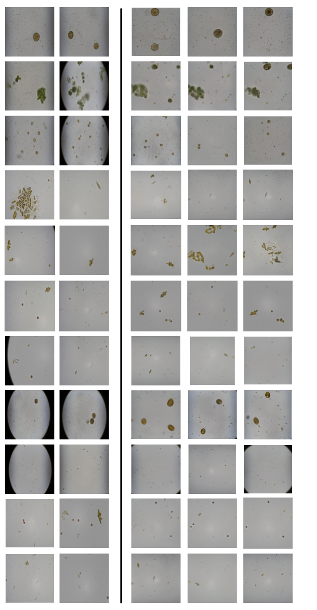
Qualitative Comparison. Figure 2 shows a visual comparison of the real algae images and the synthetic generated algae for each GAN model trained in this investigation. Based on visual inspection, conclusions can be made about each model’s effectiveness. Figure 2(a) shows the results from the ProjectedGAN model. All the generated images are entirely blank, implying that the GAN had experienced mode collapse. In contrast, the generated images from FastGAN in Figure 2(b) are somewhat similar to the real images in Figure 2(d), however, the noise within the generated images is still apparent. Lastly, Figure 2(c) shows the results from the StyleGANv2 model, and it is clear that the generated images are very similar to the real images.

Image Quality Metric Comparison. Beyond a strictly visual comparison, both the image quality and computational metrics can be seen in Table 1. When comparing the image quality metrics, the StyleGANv2 model yielded the lowest FID and KID scores by a significant margin compared to the other GAN models. The lowest FID score from the StyleGANv2 was 29.330, compared to 130.201 and 113.107 from the FastGAN and ProjectedGAN, respectively. The lowest KID score from the StyleGANv2 was 0.014 compared to 0.083 from the FastGAN and 0.050 from the ProjectedGAN. Therefore, it can be concluded that the quality of generated images from the StyleGAN was about four to five times better than that of the other tested GANs.

Computational Metric Comparison. Although the StyleGANv2 model can generate the highest fidelity images; it is at the expense of longer training times and more extensive computational requirements. For example, it took over two days to train the StyleGAN2 model for three million iterations using a 512x512 resolution dataset on a dual RTX 2080 Ti and over eight days to train for 824,000 iterations using a 1024x1024 resolution dataset on a single GTX TITAN X GPU. Conversely, the FastGAN model trains the fastest but converges at the highest FID and KID values. Lastly, the ProjectedGAN model took around two to four days to train for about 1,000,000 iterations on the GTX GPU; however, in both instances, the GAN had clearly failed during training.

Investigating Potential GAN Failure

Since the StyleGANv2 yielded the best results in this investigation, the model was further tested to ensure that images generated by the GAN are novel. When working with GAN models trained with a limited number of training images, the model may potentially memorize images from the dataset instead of generating novel images. Therefore, we checked the nearest neighbours of generated images in the real dataset, nearness being measured in (a) pixel space and (b) feature space. We provide one example each in Figure 3, the nearest-neighbour analysis of the StyleGANv2 model shows that the synthetic images are indeed novel.

Conclusions & Future Works

This work provides a framework for integrating synthetic datasets into the critical application of HAB monitoring. We investigate the effectiveness of GANs in generating high-resolution novel photorealistc synthetic phytoplankton images from a small dataset of real images. We explored three SOTA GAN architectures, and found StyleGANv2 to be quite reliable qualitatively and quantitatively.

Given the outcomes of this paper, the immediate future work includes (1) labelling the real and generated datasets, and then (2) training a classifier with the original and the combined original and new datasets to evaluate model performance. Finally, careful consideration must be taken on how these models are deployed in the field to ensure reliable and consistent predictions are provided to end users, such as aquaculture farmers. This will help mitigate the impacts of climate change by contributing a key step towards quick and accurate HAB monitoring.

Acknowledgements

This research was funded by the Waterloo AI Institute and the Mitacs Accelerate Program. The dataset was provided by Blue Lion Labs, and the computing resources were provided by the Vision and Image Processing (VIP) Lab at the University of Waterloo.

References

[\citeauthoryearAbdullah et al.2022] Abdullah; Khan, Z.; Mumtaz, W.; Mumtaz, A. S.; Bhattacharjee, S.; and Kim, H.-C. 2022. Multiclass-classification of algae using dc-gan and transfer learning. In 2022 2nd International Conference on Image Processing and Robotics (ICIPRob), 1–6.
[\citeauthoryearArmijo et al.2020] Armijo, J.; Oerder, V.; Auger, P.-A.; Bravo, A.; and Molina, E. 2020. The 2016 red tide crisis in southern chile: Possible influence of the mass oceanic dumping of dead salmons. Marine Pollution Bulletin 150:110603.
[\citeauthoryearBińkowski et al.2018] Bińkowski, M.; Sutherland, D. J.; Arbel, M.; and Gretton, A. 2018. Demystifying mmd gans.
[\citeauthoryearBrooks et al.2016] Brooks, B. W.; Lazorchak, J. M.; Howard, M. D.; Johnson, M.-V. V.; Morton, S. L.; Perkins, D. A.; Reavie, E. D.; Scott, G. I.; Smith, S. A.; and Steevens, J. A. 2016. Are harmful algal blooms becoming the greatest inland water quality threat to public health and aquatic ecosystems? Environmental Toxicology and Chemistry 35(1):6–13.
[\citeauthoryearBustos, Ramírez, and Rudolf2021] Bustos, B.; Ramírez, M. I.; and Rudolf, M. 2021. Scalar Implications of Circular Economy Initiatives in Resource Peripheries, the Case of the Salmon Industry in Chile. Cham: Springer International Publishing. 183–200.
[\citeauthoryearGoodfellow et al.2014] Goodfellow, I. J.; Pouget-Abadie, J.; Mirza, M.; Xu, B.; Warde-Farley, D.; Ozair, S.; Courville, A.; and Bengio, Y. 2014. Generative adversarial networks.
[\citeauthoryearGranéli and Turner2006] Granéli, E., and Turner, J. 2006. Ecology of harmful algae.
[\citeauthoryearHeusel et al.2017] Heusel, M.; Ramsauer, H.; Unterthiner, T.; Nessler, B.; and Hochreiter, S. 2017. Gans trained by a two time-scale update rule converge to a local nash equilibrium.
[\citeauthoryearHuang and Belongie2017] Huang, X., and Belongie, S. 2017. Arbitrary style transfer in real-time with adaptive instance normalization.
[\citeauthoryearKarras et al.2019] Karras, T.; Laine, S.; Aittala, M.; Hellsten, J.; Lehtinen, J.; and Aila, T. 2019. Analyzing and improving the image quality of stylegan.
[\citeauthoryearLi et al.2021] Li, Y.; Guo, J.; Guo, X.; Hu, Z.; and Tian, Y. 2021. Plankton detection with adversarial learning and a densely connected deep learning model for class imbalanced distribution. Journal of Marine Science and Engineering 9(6).
[\citeauthoryearLiu et al.2021] Liu, B.; Zhu, Y.; Song, K.; and Elgammal, A. 2021. Towards faster and stabilized gan training for high-fidelity few-shot image synthesis.
[\citeauthoryearMcQuatters-Gollop et al.2017] McQuatters-Gollop, A.; Johns, D. G.; Bresnan, E.; Skinner, J.; Rombouts, I.; Stern, R.; Aubert, A.; Johansen, M.; Bedford, J.; and Knights, A. 2017. From microscope to management: The critical value of plankton taxonomy to marine policy and biodiversity conservation. Marine Policy 83:1–10.
[\citeauthoryearMirza and Osindero2014] Mirza, M., and Osindero, S. 2014. Conditional generative adversarial nets. arXiv preprint arXiv:1411.1784.
[\citeauthoryearMontes et al.2018] Montes, R. M.; Rojas, X.; Artacho, P.; Tello, A.; and Quiñones, R. A. 2018. Quantifying harmful algal bloom thresholds for farmed salmon in southern chile. Harmful Algae 77:55–65.
[\citeauthoryearMoore et al.2008] Moore, S.; Trainer, V.; Mantua, N.; Parker, M.; Laws, E.; Backer, L.; and Fleming, L. 2008. Impacts of climate variability and future climate change on harmful algal blooms and human health. BioMed Central Ltd.
[\citeauthoryearPersson et al.2022] Persson, D.; Nødtvedt, A.; Aunsmo, A.; and Stormoen, M. 2022. Analysing mortality patterns in salmon farming using daily cage registrations. Journal of Fish Diseases 45(2):335–347.
[\citeauthoryearRadford, Metz, and Chintala2016] Radford, A.; Metz, L.; and Chintala, S. 2016. Unsupervised representation learning with deep convolutional generative adversarial networks. In Bengio, Y., and LeCun, Y., eds., 4th International Conference on Learning Representations, ICLR 2016, San Juan, Puerto Rico, May 2-4, 2016, Conference Track Proceedings.
[\citeauthoryearSalido et al.2020] Salido, J.; Sánchez, C.; Ruiz-Santaquiteria, J.; Cristóbal, G.; Blanco, S.; and Bueno, G. 2020. A low-cost automated digital microscopy platform for automatic identification of diatoms. Applied Sciences 10(17).
[\citeauthoryearSauer et al.2021] Sauer, A.; Chitta, K.; Müller, J.; and Geiger, A. 2021. Projected gans converge faster.
[\citeauthoryearWang et al.2004] Wang, Z.; Bovik, A.; Sheikh, H.; and Simoncelli, E. 2004. Image quality assessment: from error visibility to structural similarity. IEEE Transactions on Image Processing 600–612.
[\citeauthoryearWang et al.2017] Wang, C.; Yu, Z.; Zheng, H.; Wang, N.; and Zheng, B. 2017. Cgan-plankton: Towards large-scale imbalanced class generation and fine-grained classification. In 2017 IEEE International Conference on Image Processing (ICIP), 855–859.
[\citeauthoryearWells et al.2020] Wells, M. L.; Karlson, B.; Wulff, A.; Kudela, R.; Trick, C.; Asnaghi, V.; Berdalet, E.; Cochlan, W.; Davidson, K.; De Rijcke, M.; Dutkiewicz, S.; Hallegraeff, G.; Flynn, K. J.; Legrand, C.; Paerl, H.; Silke, J.; Suikkanen, S.; Thompson, P.; and Trainer, V. L. 2020. Future hab science: Directions and challenges in a changing climate. Harmful Algae 91:101632. Climate change and harmful algal blooms.
[\citeauthoryearYang et al.2017] Yang, S.; Xie, L.; Chen, X.; Lou, X.; Zhu, X.; Huang, D.; and Li, H. 2017. Statistical parametric speech synthesis using generative adversarial networks under a multi-task learning framework.
[\citeauthoryearZhu et al.2017] Zhu, J.-Y.; Park, T.; Isola, P.; and Efros, A. A. 2017. Unpaired image-to-image translation using cycle-consistent adversarial networks. In Proceedings of the IEEE international conference on computer vision, 2223–2232.

Towards Generating Large Synthetic Phytoplankton Datasets
for Efficient Monitoring of Harmful Algal Blooms

Abstract

Introduction

Related Works