A Multi-Dimensional Matrix Pencil-Based
Channel Prediction Method for
Massive MIMO with Mobility
Abstract
This paper addresses the mobility problem in massive multiple-input multiple-output systems, which leads to significant performance losses in the practical deployment of the fifth generation mobile communication networks. We propose a novel channel prediction method based on multi-dimensional matrix pencil (MDMP), which estimates the path parameters by exploiting the angular-frequency-domain and angular-time-domain structures of the wideband channel. The MDMP method also entails a novel path pairing scheme to pair the delay and Doppler, based on the super-resolution property of the angle estimation. Our method is able to deal with the realistic constraint of time-varying path delays introduced by user movements, which has not been considered so far in the literature. We prove theoretically that in the scenario with time-varying path delays, the prediction error converges to zero with the increasing number of the base station (BS) antennas, providing that only two arbitrary channel samples are known. We also derive a lower-bound of the number of the BS antennas to achieve a satisfactory performance. Simulation results under the industrial channel model of 3GPP demonstrate that our proposed MDMP method approaches the performance of the stationary scenario even when the users’ velocity reaches 120 km/h and the latency of the channel state information is as large as 16 ms.
Index Terms:
Massive MIMO, mobility, channel prediction, CSI delay, matrix pencil, MDMP prediction method, channel structure.I Introduction
Massive multiple-input multiple-output (MIMO) technology is playing a key role in enhancing the spectral efficiency of the fifth generation (5G) mobile communication systems [2]. Compared to the conventional MIMO, massive MIMO greatly improves the capacity and reliability of mobile communication system by deploying more antenna elements at the base station (BS) [3].
Theoretically, the performance of massive MIMO is governed by the accuracy of the channel state information (CSI). In practice, there are several causes of inaccurate CSI, including pilot contamination [4], imperfect CSI feedback in frequency division duplexing (FDD) mode [2], the mobility problem [5] (or the “curse of mobility”), etc. Although a rich body of literature has addressed the problems of pilot contamination and CSI feedback in FDD, e.g., in [6, 7, 8, 9], the mobility problem has received relatively little attention so far, and is still a challenging problem to be solved. Such a problem mainly results from the mobility of user equipment (UE) and the delay of CSI [5]. The movement of the UE makes the estimation of CSI outdated and unusable for multi-user precoding, particularly in high-mobility scenario with large CSI delay. Some papers have focused on the effect of CSI delay and prove that it is harmful for the spectral efficiency performance of massive MIMO [10, 11, 12, 13].
One way to overcome this problem is by channel prediction, which has been investigated in the literature. The work in [14] proposes a spatial-temproal basis expansion model (ST-BEM) method to predict the downlink (DL) channel. The authors of [15] propose a compressed sensing channel prediction method. An efficient approximated maximum likelihood estimator is proposed in [16]. However, the aforementioned literature generally assumes the channel parameters are time-invariant, which might be questionable in practical mobility scenarios. The time-varying delay in Wi-Fi communication scenario is studied in [17], where the authors propose an iterative channel estimator basing on a two-dimensional (2-D) subspace spanned by the discrete prolate spheroidal (DPS) sequence. The DPS sequence has less spectrum leakage than the discrete Fourier transform (DFT) sequence. However, the DPS sequence needs to meet two specific requirements in applications: and , where is the maximum Doppler, denotes the maximum delay, is the duration of sample, and represents the sub-carrier spacing. These requirements might not be easily full-filled in practice.
Recently, machine-learning (ML) and neural network (NN) algorithms, such as recurrent NN, conventional NN and deep NN, have been applied to predict the channel through the trained network with the historical data [18, 19, 20, 21]. The authors in [21] propose a data-driven channel prediction method by adopting complex-valued NN algorithm. However, these algorithms usually need enormous data, which cannot be collected easily in realistic systems. Additionally, these algorithms may perform well in static and low-mobility scenarios, yet they might not achieve the expected performance in high-mobility scenario due to the long training time. Moreover, the trained network may not perform ideally in the varying environment, due to the challenge of network generalization.
By transforming the wideband channel into angular-delay domain, the paper [5] proposes a Prony-based angular-delay domain (PAD) prediction method and proves that it can overcome the problem of CSI aging. However, it does not take the effect of time-varying path delay into consideration and assumes the CSI delay to be an integral multiple of the pilot interval. To the best of our knowledge, the realistic effect of time-varying path delay is overlooked in most of the existing literature. Such an effect makes the path delay difficult to track and leads to the distortion of the traditional time-domain multipath channel structure.
In order to break the limitations above and tackle the mobility problem, we propose a novel matrix pencil (MP) based super-resolution channel prediction method. The super-resolution property of our method comes from the super-accurate parameters estimated by MP algorithm. In the literature, some papers adopt MP algorithm to estimate channel parameters. In [22] the authors adopt 2-D MP algorithm to estimate 2-D frequencies. The work in [23] estimates the path angle and delay in the IEEE 802.11ac context. The elevation angle of departure (EOD), azimuth angle of departure (AOD) and delay are estimated in [24]. Compared to other traditional super-resolution algorithms, e.g., multiple signal classification (MUSIC) [25] and estimation of signal parameters via rational invariance techniques (ESPRIT) [26], MP algorithm has some distinct advantages: it does not search and find peak value in space, and it needs less channel samples. However, the traditional MP algorithm cannot be directly applied to solve the mobility problem of massive MIMO, because of the time-varying path delay and the multi-dimensional structure of the wideband massive MIMO channel.
In order to achieve more accurate channel predictions in this paper, we extend the traditional MP method to multi-dimensional algorithm that extracts the EOD, AOD, time-varying delay and Doppler simultaneously. Specifically, we first introduce a three-dimensional (3-D) MP algorithm to estimate the EOD, AOD, and delay on the angular-frequency domain, and then put forward another 3-D MP algorithm to estimate the EOD, AOD and Doppler on the angular-time domain. Based on the super-resolution property of the estimated EOD and AOD, we propose a pairing algorithm to pair the path delay and Doppler. The future CSI is reconstructed with the estimated parameters. To the best of our knowledge, our proposed multi-dimensional matrix pencil (MDMP) method is the first attempt to estimate the EODs, AODs, Doppler and the time-varying delays of multiple paths simultaneously.
The contributions of this paper are summarized as follows:
- •
We propose a super-resolution MDMP prediction method to address the mobility problem with time-varying path delays, which estimates the multipath EODs, AODs, delays and Doppler simultaneously through angular-time-domain and angular-frequency-domain structures of the channel. Compared to the traditional methods, significant gains of our proposed method are confirmed in simulations.
- •
We prove that the prediction error of the MDMP method converges to zero in mobility scenario with arbitrary CSI delay, when the number of the BS antennas and the bandwidth are large enough. Our proposed method breaks the limitation of the PAD method whose CSI delay is an integral multiple of the pilot interval.
- •
We also prove that the prediction error converges to zero providing that only two arbitrary samples are known, when the number of the BS antennas is large enough. Our proposed MDMP method does not necessarily require the samples to be neighboring ones, yet it is a common assumption in most existing works.
- •
We derive a lower-bound of the number of the BS antennas in a wideband channel to give a satisfactory performance of the MDMP method. The lower-bound is correlated with the number of samples. As the number of samples increases, the lower-bound decreases.
This paper is organized as follows: Sec. II introduces the channel model. In Sec. III, MDMP prediction method is proposed. The performance of MDMP method is analyzed in Sec. IV. The simulation results are shown in Sec. V, and Sec. VI concludes the paper.
Notations: We use boldface to represent vectors and matrices, where , , and denote zero matrix, identity matrix, anti-identity matrix and all-ones matrix. Let , , , and denote the transpose, conjugate, conjugate transpose, inverse and Moore-Penrose pseudoinverse of the matrix , respectively. denotes the number of the elements in a set. denotes the rank of a matrix. stands for the Frobenius norm. and take the real and imaginary components of a complex number. is the expectation operation. denotes the diagonal operation of a matrix. is the extending matrix of and . and denote the Hadamard product and Kronecker product of and .
II Channel Model
We consider a wideband time division duplexed (TDD) massive MIMO system, where a BS serves multiple UEs. In such a system, the BS estimates the CSI from the uplink (UL) pilot, and the DL CSI is acquired based on channel reciprocity.
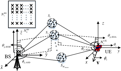
Fig. 1 illustrates the channel between the BS and the UE. In most 5G commercial systems, the BS is equipped with a uniform planar array (UPA), which consists of columns and rows of antenna elements. The numbers of the BS antennas and the UE antennas are respectively and . There are different clusters, which are denoted by , . Each cluster contains many scattering rays. The UL and DL channels share the same bandwidth, which is composed of subcarriers with spacing .
The DL MIMO channel between the BS and the UE is expressed as , where denotes the channel frequency response between the -th column and the -th row of the BS antenna array and the -th antenna of the UE, and is modeled as [27]
| (1) |
where denotes the number of paths, and is the complex amplitude of the -th path. Also, is the wavelength, where is the central carrier frequency and is the speed of light. Furthermore, and denote the spherical unit vectors of the UE and the BS, and are expressed as
| (2) |
| (3) |
where , , and are the elevation angle of arrival (EOA), azimuth angle of arrival (AOA), EOD and AOD, respectively. Additionally, and are the location vectors of the BS and the UE antennas:
| (4) |
where is the horizontal antenna spacing, and is the vertical antenna spacing. Moreover, represents the Doppler, and is the velocity vector of the UE:
| (5) |
where is the speed, is the elevation angle of velocity, and is the azimuth angle of velocity. The -th path delay is time-varying and modeled as [27]
| (6) |
where is the initial value, and denotes the changing rate of the path delay. Notice that, besides the time domain, Doppler also has an effect on the frequency domain. The 3-D steering vector is expressed as
| (7) |
where and are and for simplicity. Furthermore, and denote the spatial signatures in the directions of and , which are expressed as
| (8) |
| (9) |
Let denote the channel between all BS antennas and the -th UE antenna at time and frequency :
| (10) |
In the time domain, the channels at all subcarriers are expressed as
| (11) |
where is the frequency of the -th subcarrier:
| (12) |
Based on the angular-frequency-domain channel structure, is rewritten as
| (13) |
where contains the 3-D steering vectors of all paths:
| (14) |
The frequency-domain matrix is expressed as
| (15) |
where denotes the delay response vector at the -th subcarrier:
| (16) |
The diagonal matrix is expressed as
| (17) |
According to the angular-time-domain channel structure, is also rewritten as
| (18) |
where is a diagonal matrix:
| (19) |
The matrix is composed of the initial delay response vectors at all subcarriers:
| (20) |
where is for the -th subcarrier:
| (21) |
The time-domain matrix is expressed as
| (22) |
where , is defined as:
| (23) |
Notice that Eq. (18) is different from the result in [5], as we simultaneously consider the effect of Doppler on time domain and frequency domain. The multipath delays, angles and Doppler will be estimated jointly by our proposed MDMP method in the next section.
III The Proposed MDMP Prediction Method
In this section, we introduce our proposed MDMP super-resolution method for channel prediction. In general, our approach first estimates the EOD, AOD, delay, and Doppler information by exploiting the angular-frequency-domain and angular-time-domain structures of the channel, and then performs a path pairing procedure to determine the corresponding parameters of the paths. Finally the BS predicts the CSI by reconstructing the future channel with the estimated parameters. To ease the exposition, we briefly introduce here the derivations in Sec. III-A and Sec. III-B. Since Sec. III-A and Sec. III-B have similar derivations, we take Sec. III-A for example. The derivation mainly contains five steps, i.e., generating the 3-D MP matrix from the channels, transforming the 3-D complex MP matrix to a real matrix, determining the number of paths, estimating the path delays, and estimating the EODs and the AODs.
III-A The 3-D Angle-Delay Estimation
We first generate a 3-D MP matrix. For ease of exposition, we start with the one-dimensional (1-D) setting of the matrix pencil method, and then move on to the 2-D and 3-D cases. More specifically, we first generate a 1-D MP matrix only containing the information of , by windowing the BS antenna panel in the horizontal direction. Then, we generate a 2-D MP matrix by adding the second window in the vertical direction of the BS antenna panel, which also contains the information of . Finally, based on the 2-D MP matrix, we generate a 3-D MP matrix by adding the third window in the frequency domain, which contains the information of path delay. More details will be shown below.
Based on the angular-frequency-domain channel structure, a 1-D MP matrix is generated by sliding a horizontal window within the BS antenna panel. Such a MP matrix is defined as
| (24) |
which is composed of the channels between the -th UE antenna and all horizontal antennas in the -th row of the BS antenna panel at the -th subcarrier, and is the pencil size that satisfies . Based on Eq. (13), the 1-D MP matrix is rewritten as
| (25) |
where the -th column of and the -th row of , are the steering vectors of two subsets of antenna array with size and in the BS antenna panel, respectively. The two matrices and are defined as
| (26) |
| (27) |
where , . The matrix contains the phase differences between two neighboring subcarriers for the paths:
| (28) |
Likewise, denotes the matrix of the phase differences between two neighboring vertical BS antennas for the paths:
| (29) |
The matrix is defined as
| (30) |
By adding a new window along the vertical direction of the BS antenna panel, a 2-D MP matrix is introduced
| (31) |
which is composed of the channels between the -th UE antenna and all BS antennas at the -th subcarrier, and contains the angular information of the paths. The corresponding pencil size is denoted by that satisfies . Substituting Eq. (25) into Eq. (31), is rewritten as
| (32) |
where the -th column of and the -th row of are the 3-D steering vectors of two subsets of antenna array with size and on the BS antenna panel, respectively. They are defined as
| (33) |
| (34) |
Adding the third window in the frequency domain, a 3-D MP matrix is generated from and expressed as
| (35) |
where is the pencil size that satisfies . The matrix is composed of the channels between the -th UE antenna and all BS antennas at all subcarriers, and also contains the angular and delay information of the paths. For notational simplicity, we define and . According to the channel angular-frequency-domain structure in Eq. (13), is rewritten as
| (36) |
where and are defined as
| (37) |
| (38) |
The physical meaning of is the EOD-AOD steering vectors of a subset of antenna array with size on the BS antenna panel at the -th subcarrier of the paths. Likewise, is the EOD-AOD steering vectors of a subset of antenna array with size on the BS antenna panel at the -th subcarrier for the paths. The 3-D MP matrix contains the information of multipaths, if its rank satisfies . In this case, the three pencil sizes yield
| (39) |
Then, we transform the 3-D MP matrix to a real matrix by the unitary matrix pencil (UMP) method [28], which reduces the computational complexity without losing accuracy. The real matrix is transformed by
| (40) |
where
| (41) |
We define and as two unitary matrices depending on the size of and . Taking for example, if is even,
| (42) |
and if it is odd,
| (43) |
Next we will determine the number of paths by the singular value decomposition (SVD) of : , where , , and . Without loss of generality, we assume the diagonal elements of are in non-increasing order. To determine the number of non-negligible paths, we define a set
| (44) |
where the positive threshold is close to zero. The number of non-negligible paths .
Hereinafter, we estimate the path delay, which contains two substeps, i.e., generating a real matrix, and the EVD. We first define a matrix , which is generated by selecting the columns from . A real matrix related to the path delays is defined as
| (45) |
where and . The unitary matrix only depends on the size , and is expressed as Eq. (42) or Eq. (43). We also introduce a matrix , which contains the delay information:
| (46) |
The two matrices and are similarity matrices that share the same eigenvalues [28]. Then, the path delay will be estimated by the EVD of : , where is an eigenvectors collection of . Since and are similarity matrices, can be calculated by . According to the angular-frequency-domain channel structure in Eq. (13), the estimated diagonal elements in may reflect the multipath delay phase differences between two neighboring subcarriers. Thus, the -th path delay is estimated as
| (47) |
where denotes the -th estimated diagonal element of . Moreover, the delay changing rate is estimated with two different time samples:
| (48) |
Up to now, the multipath delays have been estimated. Next, we estimate the multipath EODs and AODs mainly by two substeps, i.e., introducing some shuffling matrices, generating two real matrices related to the EODs and the AODs. Since contains the angular information of the paths, we only need to permute to generate two new 3-D MP matrices and . First, four shuffling matrices , , and are introduced as
| (49) |
| (50) |
| (51) |
| (52) |
where , is an unit vector with the -th element being one. Permuted from , the two matrices and are expressed as and , respectively. Notice that in practice, the two 3-D MP matrices and , as well as the two shuffling matrices and , are not needed. In fact, the EODs and the AODs might be estimated by only introducing and .
Then, we will focus on the generation of the two real matrices related to the EODs and the AODs. By following a similar procedure to generate from , i.e., from Eq. (40) to Eq. (45), we may obtain two real matrices and , which are generated from and respectively. The matrices and are defined by
| (53) |
| (54) |
where , , , and . The two unitary matrices and are defined in Eq. (42) or Eq. (43) according to their sizes and .
Define two real diagonal matrices and , which contain the angular information
| (55) |
| (56) |
The diagonal elements in reflect the phase differences between the two neighboring antenna elements in the horizontal direction of the BS antenna panel of the paths. Likewise, reflects the phase differences between the two neighboring antenna elements, in the vertical direction of the BS antenna panel for the paths.
Finally, we will estimate the EODs and the AODs as follows: The two real matrices and are similar to and , respectively, i.e., and share the same eigenvalues, and also share the same eigenvalues. Thus, we may obtain and via the EVDs of and . Note that , , and share the same eigenvectors, since and are simply permuted versions of . More specifically, we may denote the EVDs by and , where contains the eigenvectors of . As a result, and are calculated as and . The EOD and the AOD are estimated by
| (57) |
| (58) |
where and denote the -th estimated diagonal elements of and , respectively. So far, the EODs, AODs and delays have been estimated by our proposed 3-D angle-delay estimation scheme, which is summarized in Algorithm 1. Notice that as an input of Algorithm 1 is a historical sample obtained from the UL sounding reference signal (SRS). With Algorithm 1, we will estimate the channel parameters, which are used for reconstructing and predicting the future DL channel.
We now analyze the computational complexity of this algorithm in terms of time and memory. The time complexity is dominated by step 3 - step 8. The complexity of step 3 is . The main complexity of step 4 is the SVD, i.e., . Step 5 contains the matrix inversion and multiplications, and has a complexity order of . In step 6, the computation complexity is dominated by the EVD, i.e., . The complexity of step 7 is , which mainly contains the matrix inversion and multiplication. Similar to step 6, step 8 has a complexity order of . According to the conditions of pencil sizes in Eq. (39), we may obtain the global time complexity of Algorithm 1 as . Then, the memory complexity of Algorithm 1 is dominated by step 3, i.e., the two matrices and in step 3 lead to the total memory complexity order of .
III-B The 3-D Angle-Doppler Estimation
With the angular and delay information obtained in Sec. III-A, we now estimate the multipath angles and Doppler in this section. Since the duration of the channel sample is , the -th sample time is denoted by . Similar to Sec. III-A, we start by defining a 3-D MP matrix as
| (59) |
where is the number of samples, and is the pencil size satisfying . The matrix is composed of the channels between the -th UE antenna and all BS antennas at the first subcarrier and all sample times. For simplicity, we define and . The 2-D MP matrix , consists of the channels between the -th UE antenna and all BS antennas at the first subcarrier and the -th sample. We rewrite as
| (60) |
where denotes the phase differences between two neighboring samples of the paths:
| (61) |
where
| (62) |
The matrix is defined as
| (63) |
where and are shown in Eq. (19) and Eq. (21). According to the angular-time-domain channel structure in Eq. (18), is rewritten as
| (64) |
where and are defined as
| (65) |
| (66) |
The physical meaning of , is the 3-D steering vectors of a subset of antenna array with size on the BS antenna panel at the -th sample. Likewise, , is the 3-D steering vectors of a subset of antenna array with size on the BS antenna panel at the -th sample.
The three pencil sizes in yield
| (67) |
By following the similar estimation procedures of Sec. III-A, we then transform to a real matrix as . The step of determining the number of paths is not needed, because this work has been finished in Sec. III-A. Next, we will estimate the parameter by generating a real matrix and the EVD. More specifically, a real matrix related to Doppler is given by
| (68) |
where , and . The two unitary matrices and depending on the size of and , are expressed as Eq. (42) or Eq. (43). Perform the SVD of : . We select the columns from as , which follows the similar procedure of in Sec. III-A. The matrix and a real diagonal matrix are similarity matrices, and share the same eigenvalues. The matrix containing the Doppler information is defined as
| (69) |
The diagonal elements in reflect the phase differences between two samples of the paths.
Until now, the real matrix has been generated, and the following step is the EVD. We perform the EVD of : , where is composed of the eigenvectors of . The matrix is calculated as . The parameter is thus estimated by
| (70) |
where denotes the -th estimated diagonal element of . Likewise, we will estimate the EODs and the AODs as follows: The two real matrices related to the EODs and the AODs are given by
| (71) |
| (72) |
where , , , and . Define and as two new shuffling matrices that share the similar expressions with and in Eq. (49) and Eq. (51). The two shuffling matrices and are generated by replacing the parameter with in Eq. (49) and Eq. (51). The two matrices and are similar to two real diagonal matrices and :
| (73) |
| (74) |
which are given by and . The EOD and the AOD are estimated by
| (75) |
| (76) |
where and denote the -th estimated diagonal elements of and .
The procedures of our proposed 3-D angle-Doppler estimation scheme are summarized in Algorithm 2. Similar to the time and memory complexity analysis of Algorithm 1, we may obtain the time complexity of Algorithm 2 as , and the memory complexity as .
III-C The Proposed Angle-Delay-Doppler Pairing Scheme
We propose to pair the angles, delay, and Doppler of the paths, with the super-resolution property of the angle estimation. Let some vectors , , , , , and denote the corresponding estimated parameters of multipaths. A pairing matrix is defined to map the relationship between and as
| (77) |
where , is a unit vector with only one element being one. Denote the -th row of as . By solving the minimization problem
| (78) |
we may obtain . Specifically, is the error vector between and , and is the error vector between and . The row index of satisfying the minimize value of is the row index of the only non-zero entry in .
By reordering the entries of with the pairing result, the Doppler is obtained as
| (79) |
Now, and are paired correctly and associated with the corresponding paths. With the estimated parameters, the future channel at time can be reconstructed as .
Our proposed MDMP method is summarized in Algorithm 3. The step 3 - step 6 of Algorithm 3 has a time complexity order of , and a memory complexity order of . The time complexity of channel reconstruction in step 7 is . The memory complexity of step 7 is . The time and memory complexity of the MDMP method are primarily determined by Algorithm 1 and Algorithm 2. Therefore, the global time complexity of the MDMP method is . The MDMP method has a global memory complexity order of . The PAD method in [5] has a complexity order of , where , and denote the prediction order of the PAD method and the number of the predicted samples. The MDMP method may have a larger time complexity compared to the PAD method. However, the MDMP method has better performance and is applicable in more general settings, i.e., the CSI delay does not have to be an interval multiple of the pilot interval, the historical channel samples are not necessarily neighboring ones. The detailed proofs will be shown in the next section.
IV Performance Analysis of the MDMP Prediction Method
In this section, we show the performance analysis of our proposed MDMP prediction method. Denote the observation sample at time by . The vectorized forms of , and are denoted respectively by , , and , i.e., , and . Before the asymptotic performance analysis, we introduce an assumption.
Assumption 1.
The observation sample yields
| (80) |
where is the independent identically distributed (i.i.d.) Gaussian white noise with zero mean and element-wise variance . As , the variance converges to zero, such that:
| (81) |
Remarks: This technical assumption means the normalized channel sample error converges to zero when the number of the BS antennas and the bandwidth increase. In fact, the condition of Eq. (81) can be achieved even in the multi-user multi-cell scenario with pilot contamination, by some non-linear signal processing technologies [29].
For simplicity, we also introduce a vector in Definition 1.
Definition 1.
Define a vector containing the parameters of multipaths as
| (82) |
where , .
Theorem 1.
Under Assumption 1, for an arbitrary CSI delay , the asymptotic performance of MDMP prediction method yields:
| (83) |
providing that the pencil sizes satisfy , , , and .
Proof.
The proof can be found in Appendix A.
Remarks: Theorem 1 indicates that the channel prediction error converges to zero when the number of the BS antennas and the bandwidth are large. Note that the CSI delay in Theorem 1 does not have to be an integral multiple of the pilot interval, which indicates our proposed MDMP method is more general than the PAD method in [5] because the PAD achieves asymptotically error-free performance when the CSI delay is an integral multiple of the channel sampling interval.
If , the least number of samples in Theorem 1 should satisfy . The number of paths might be large in rich scattering environment. In such cases, Theorem 1 indicates that we may need a large number of samples to achieve asymptotically error-free prediction. In the following, we will show the asymptotic performance of the prediction error with only two arbitrary samples known.
Theorem 2.
Under Assumption 1, if the EOD and the AOD satisfy , , the number of subcarriers satisfies , and the configuration of the BS antennas satisfies and , then with only two arbitrary samples and known, the asymptotic performance of the MDMP prediction method yields:
| (84) |
Proof.
The proof can be found in Appendix B.
Remarks: Theorem 2 requires that the angles of any two paths are different, which is a stronger assumption than in Theorem 1. However a better result is obtained since only two samples are needed. Note that the two samples are not necessarily neighboring ones, which is also more general than the PAD method.
In Theorem 1 and Theorem 2, the conditions of the BS antennas, e.g., and , ensure the rank of the 3-D MP matrices satisfy . If and , the least number of the BS antennas is , which seems to be large. Next, by assuming known, we derive a lower-bound of the BS antennas to give a satisfactory performance. In order to do so, we introduce two functions.
Definition 2.
Define two functions and .
| (85) |
where and satisfy
| (86) |
and . The other function is defined as
| (87) |
with
| (88) |
Next, we derive a lower-bound of the number of the BS antennas in Proposition 1 to achieve a satisfactory performance. For an arbitrary given , we derive the bound of the total number of the BS antennas . In a wideband system, and usually satisfy . According to Eq. (39) and Eq. (67), the lower-bound of the number of the BS antennas is determined by in Eq. (67). The lower-bound of consists of two sub-bounds and , where is derived from the 3-D MP matrix in estimating Doppler, and is derived from the 3-D MP matrix in estimating angles.
Proposition 1.
In a wideband channel, for a given , a lower-bound of the number of the BS antennas is given as
| (89) |
where
| (90) |
and , are defined as
| (91) |
| (92) |
and , , and . The value is defined as
| (93) |
where
| (94) |
and
| (95) |
| (96) |
Proof.
The proof can be found in Appendix C.
Remarks: In Proposition 1, for a given , we derive the lower-bound of . Such a bound means that the MDMP method does not work if the BS antenna configuration cannot satisfy the lower-bound. As a remedy, the lower-bound can be made smaller to satisfy the antenna configuration, by increasing the number of channel samples . Note that if is given, the lower-bound of can also be derived. The detailed derivation is omitted.
V Numerical Results
In this section, the simulation results of our proposed method are shown. The clustered delay line (CDL) channel model of 3GPP is adopted. The number of scattering clusters is 9. Each cluster contains 20 rays and the total number of propagation paths is 180. According to [27], the -th path delay is modeled as , where is the cluster delay, and denotes the initial delay and is modeled as a spatially random variable related to the correlation distance. The root mean square (RMS) angular spreads of AOD, EOD, AOA and EOA are , , and , respectively. The main simulation parameters are listed in Table I. Considering the 3-D Urban Macro (3-D UMa) scenario, the UEs have certain velocity, e.g., 60 km/h and 120 km/h. The central frequency is 3.5 GHz and the bandwidth is 100 MHz, which is composed of 273 resource blocks (RBs) in frequency domain. The duration of a slot is 0.5 ms, which contains 14 OFDM symbols. One channel sample is available for each slot.
| Scenario | 3D Urban Macro (3D UMa) |
|---|---|
| Carrier frequency (GHz) | 3.5 |
| Bandwidth (MHz) | 100 (273 RBs) |
| Subcarrier spacing (kHz) | 30 |
| Number of UEs | 16 |
| BS antenna configuration | , |
| UE antenna configuration | , the polarization angles are and |
| Delay Spread (ns) | 616 |
| CSI delay (ms) | 12, 16 |
| UEs speed (km/h) | 60, 120 |
The antenna configuration is denoted by , where each antenna panel has rows and columns of antenna elements; is the number of polarizations; is the number of panels in a row and is the number of panels in a column. In the horizontal and vertical directions, the antenna spacings are and respectively. The pencil sizes such as , , and , are set as 6, 5, 137 and 15, respectively. The DL precoder is eigen-based zero-forcing (EZF) [30]. Two performance metrics are evaluated, which are the DL spectral efficiency and the prediction error. The DL spectral efficiency is calculated by , where is the number of UEs, is the signal-to-noise ratio of the -th UE, and the expectation is taken over frequency and time. The DL prediction error is defined by , where and are the predicted and exact channels, respectively, and the expectation is taken over time, frequency and UEs.
Let CDL-TID and CDL-TVD denote the simulated CDL model with time-invariant and time-varying path delay, respectively. In Fig. 2(a) and (b), we show the spectral efficiencies and prediction errors of different methods with the UEs moving at the speed of 120 km/h. In Fig. 2(a), the CSI delay is relatively large, e.g., 12 ms and 16 ms, while in Fig. 2(b), the CSI delay is within the range of 4 to 20 ms. The ideal case of the stationary setting is also shown as a reference curve labeled as “Stationary channel”, which is the upper-bound of the performance. The curves labeled with “No prediction” mean channel predictions are not carried out. In Fig. 2(a), the different performances of the PAD method in CDL-TID and CDL-TVD show that time-varying delay brings an observable decrease of the spectral efficiency. However, our proposed MDMP method is able to deal with the time-varying path delay, as it approaches the ideal case of the stationary setting in the scenario with a large CSI delay of 16 ms and high velocity level of 120 km/h.
Fig. 3 compares the spectral efficiencies of different methods with UEs moving at 60 km/h and 120 km/h, respectively. The curves labeled as “APF-RNS”, are the prediction performance of an adaptive and parameter-free recurrent neural structure (APF-RNS) [31], which uses 19 historical sequential channel samples to predict the channel at the next moment. In CDL-TVD, it can be observed that the performance of PAD method will decrease more obviously at higher velocity because of the faster varying delay and Doppler. However, our proposed MDMP method is close to the upper-bound of the stationary setting even in high-mobility scenarios.
Fig. 4 shows the spectral efficiencies of the MDMP and PAD methods with multiple-speed UEs, where every four UEs move at 30 km/h, 60 km/h, 90 km/h and 120 km/h, respectively. One may observe that our proposed MDMP method still performs well in this setting.
Fig. 5 gives the prediction errors of MDMP and PAD methods with different numbers of the BS antennas, e.g., 64, 128, 192, 256, 320 and 384. The corresponding antenna configurations are , , , , and , respectively. One may notice that the prediction error of our MDMP method decreases obviously with the increasing numbers of the BS antennas. One may notice the error floor of the MDMP method. This is because the bandwith is fixed and not large enough.
By adding a line-of-sight (LOS) path, CDL-TVD is changed to a new model named CDL-LOSTVD, which contains 181 propagation paths. The RMS angular spreads of AOD, EOD, AOA and EOA are updated to , , and , respectively. The spectral efficiencies of different methods in CDL-LOSTVD are shown in Fig. 6. It is clear that our proposed MDMP method is capable of dealing with the effect of time-varying delay in this setting, and nearly approaches the upper-bound of the stationary setting.
VI Conclusion
In this paper, we addressed the challenge of mobility under the industrial channel model with time-varying path delay in massive MIMO. We proposed a novel multi-dimension matrix pencil channel prediction method, which estimates the angles, delay and Doppler simultaneously by exploiting the angular-time-domain and angular-frequency-domain structures of the wideband massive MIMO channel. We also proposed a pairing method to associate the paths with the estimated angles, delay and Doppler by exploiting the super-resolution property of the angle estimation. In the theoretical analysis, we proved that the proposed MDMP method asymptotically achieves the error-free performance with arbitrary CSI delay, providing that only two arbitrary samples are known. We also derived a lower-bound of the number of the BS antennas for this method to work. By increasing the number of channel samples, the bound can be made lower. Simulation results demonstrated that our proposed MDMP method in high-mobility scenarios with a large CSI delay, is very close to the performance of the stationary setting.
-A Proof of Theorem 1
For ease of exposition, we will first calculate the estimations of parameters with the observation channel samples, and then we prove that the estimations of parameters converge to the exact ones.
Firstly, the channel parameters are estimated as follows: After an arbitrary CSI delay , is updated as . The channel in Eq. (13) is rewritten as
| (97) |
where is the sample noise matrix. The matrix is introduced by UE movement during , and is expressed as
| (98) |
The matrix contains multipath delay response vectors and is given by
| (99) |
where
| (100) |
Then, the 3-D MP matrix is expressed as
| (101) |
where is generated by , and
| (102) |
| (103) |
| (104) |
and
| (105) |
As , and , and contains the angular and path delay information of the paths. The SVD of is , where , , and the diagonal elements of are in non-increasing order. Without loss of generality, we let , and . We set a new threshold to determine the number of the non-negligible paths as . Define the corresponding columns of as .
We select columns from to form . Since , they may satisfy a mapping relationship as , where is a full-rank matrix. Define the first rows and the last rows from as and , respectively, which satisfy
| (106) |
where . The matrix and the diagonal matrix are similarity matrices, and share the same eigenvalues. With the UMP method, , , and are transformed to , and , respectively, where is defined as
| (107) |
and is generated from . The diagonal matrix and the matrix are introduced by
| (108) |
| (109) |
where is the columns from , and is calculated by the SVD of :
| (110) |
where , , , and . Obviously, and are similarity matrices. With the EVD of , we may estimate by , where contains the eigenvectors of . After CSI delay , the path delay is estimated as
| (111) |
where is the -th estimated diagonal element of . The changing rate of path delay is estimated by two different samples as
| (112) |
The other parameters, i.e., Doppler, EODs and AODs can also be estimated by the similar estimation procedure of , and the details are omitted. So far, the parameters have been estimated with the observation samples. Then, we derive the asymptotic performance of parameter estimations under Assumption 1.
When the number of the BS antennas and the bandwidth are large, the correlation matrix of is calculated by
| (113) |
where , , and is the expectation over the BS antennas and bandwidth. By performing the SVD of , we obtain
| (114) |
where and
| (115) |
| (116) |
Under Assumption 1, we may obtain
| (117) |
where , and
| (118) |
In other words, the -th diagonal elements in and satisfy: . According to Eq. (110), we may obtain and . According to Eq. (110), we denote the columns of as and may obtain
| (119) |
where and is a unitary vector with the -th element being . The real matrix related to path delays asymptotically converges to
| (120) |
where is generated by the sample without noise:
| (121) |
Obviously, and are similar and share the same eigenvalues. In other words, despite the observation noise, the estimation of the -th path delay asymptotically converges to the exact value, i.e.,
| (122) |
Likewise,
| (123) |
With the estimated parameters in , the channel after is reconstructed as . Then, we may obtain
| (124) |
Thus, Theorem 1 is proved.
-B Proof of Theorem 2
We first derive the least number of samples below. The 2-D MP matrix generated by the observation samples, is defined as
| (125) |
where is the noise matrix. The 3-D MP matrix is introduced by
| (126) |
where . Since and , . Therefore, and contain the angular information. Based on the expression of in Eq. (60), .
Based on Eq. (65), by applying the inequalities
| (127) |
| (128) |
with and , the rank of satisfies
| (129) |
and , since . Consequently, . Likewise, . Based on Eq. (127), satisfies:
| (130) |
| (131) |
Thus, , which still holds if .
Likewise, we may derive that the smallest number of subcarriers satisfies . The estimations of parameters can be calculated by setting and . The details are omitted. Following the similar proof procedure in Appendix -A between Eq. (113) and Eq. (122), we may prove
| (132) |
In other words, we may obtain
| (133) |
Thus, Theorem 2 is proved.
-C Proof of Proposition 1
During the procedure of Doppler estimation, according to Eq. (67), should satisfy . Under the condition , we define a Lagrange function as
| (134) |
Letting , we obtain the two extreme points of and : and , which are shown in Eq. (91) and Eq. (92). If , and are ignored. In addition, the condition of and in Eq. (86) covers three extra extreme points e.g., , , and . By substituting these extreme points into , satisfies , where is shown in Eq. (90).
Up to now, the sub-bound of Doppler estimation is derived. Next, we derive the sub-bound of angle estimation.
In the procedure of angle estimation, and satisfy
| (135) |
Based on the different sizes of , the condition of in Eq. (88) (, and ) is divided into four different conditions, i.e., i) ; ii) ; iii) ; iv) , which lead to as in Eq. (93). If , we may obtain and , shown in Eq. (95) and Eq. (96). Depending on the value of , i.e., , and , is obtained as in Eq. (94).
Finally, the lower-bound of is determined by , and Proposition 1 is proved.
References
- [1] W. Li, H. Yin, and M. Debbah, “A super-resolution channel prediction approach based on extended matrix pencil method,” in Proc. IEEE Int. Conf. Commun. (IEEE ICC), Seoul, South Korea, May 2022.
- [2] T. L. Marzetta, “Noncooperative cellular wireless with unlimited numbers of base station antennas,” IEEE Trans. Wireless Commun., vol. 9, no. 11, pp. 3590–3600, Nov. 2010.
- [3] F. Boccardi, R. W. Heath, A. Lozano, T. L. Marzetta, and P. Popovski, “Five disruptive technology directions for 5G,” IEEE Commun. Mag., vol. 52, no. 2, pp. 74–80, Feb. 2014.
- [4] J. Jose, A. Ashikhmin, T. L. Marzetta, and S. Vishwanath, “Pilot contamination and precoding in multi-cell TDD systems,” IEEE Trans. Wireless Commun., vol. 10, no. 8, pp. 2640–2651, Aug. 2011.
- [5] H. Yin, H. Wang, Y. Liu, and D. Gesbert, “Addressing the curse of mobility in massive MIMO with prony-based angular-delay domain channel predictions,” IEEE J. Sel. Areas Commun., vol. 38, no. 12, pp. 2903–2917, Dec. 2020.
- [6] H. Yin, D. Gesbert, M. Filippou, and Y. Liu, “A coordinated approach to channel estimation in large-scale multiple-antenna systems,” IEEE J. Sel. Areas Commun., vol. 31, no. 2, pp. 264–273, Feb. 2013.
- [7] R. R. Müller, L. Cottatellucci, and M. Vehkaperä, “Blind pilot decontamination,” IEEE J. Sel. Topics Signal Process., vol. 8, no. 5, pp. 773–786, Oct. 2014.
- [8] A. Adhikary, J. Nam, J. Y. Ahn, and G. Caire, “Joint spatial division and multiplexing the large-scale array regime,” IEEE Trans. Inf. Theory, vol. 59, no. 10, pp. 6441–6463, Oct. 2013.
- [9] Z. Jiang, A. F. Molisch, G. Caire, and Z. Niu, “Achievable rates of FDD massive MIMO systems with spatial channel correlation,” IEEE Trans. Wireless Commun., vol. 14, no. 5, pp. 2868–2882, May 2015.
- [10] K. T. Truong and R. W. Heath, “Effects of channel aging in massive MIMO systems,” Journal of Communications and Networks, vol. 15, no. 4, pp. 338–351, Aug. 2013.
- [11] J. Zheng, J. Zhang, E. Björnson, and B. Ai, “Impact of channel aging on cell-free massive MIMO over spatially correlated channels,” IEEE Trans. Wireless Commun., vol. 20, no. 10, pp. 6451–6466, Oct. 2021.
- [12] R. Chopra, C. R. Murthy, H. A. Suraweera, and E. G. Larsson, “Performance analysis of FDD massive MIMO systems under channel aging,” IEEE Trans. Wireless Commun., vol. 17, no. 2, pp. 1094–1108, Feb. 2018.
- [13] C. Kong, C. Zhong, A. K. Papazafeiropoulos, M. Matthaiou, and Z. Zhang, “Sum-rate and power scaling of massive MIMO systems with channel aging,” IEEE Trans. Commun., vol. 63, no. 12, pp. 4879–4893, Dec. 2015.
- [14] J. Zhao, H. Xie, F. Gao, W. Jia, S. Jin, and H. Lin, “Time varying channel tracking with spatial and temporal BEM for massive MIMO systems,” IEEE Trans. Wireless Commun., vol. 17, no. 8, pp. 5653–5666, Aug. 2018.
- [15] S. Uehashi, Y. Ogawa, T. Nishimura, and T. Ohgane, “Prediction of time-varying multi-user MIMO channels based on DOA estimation using compressed sensing,” IEEE Trans. Veh. Technol., vol. 68, no. 1, pp. 565–577, Jan. 2019.
- [16] L. Gaudio, M. Kobayashi, G. Caire, and G. Colavolpe, “On the effectiveness of OTFS for joint radar parameter estimation and communication,” IEEE Trans. Wireless Commun., vol. 19, no. 9, pp. 5951–5965, Sept. 2020.
- [17] T. Zemen, L. Bernado, N. Czink, and A. F. Molisch, “Iterative time-variant channel estimation for 802.11p using generalized discrete prolate spheroidal sequences,” IEEE Trans. Veh. Technol., vol. 61, no. 3, pp. 1222–1233, Mar. 2012.
- [18] Y. Zhu, X. Dong, and T. Lu, “An adaptive and parameter-free recurrent neural structure for wireless channel prediction,” IEEE Trans. Commun., vol. 67, no. 11, pp. 8086–8096, Nov. 2019.
- [19] J. Yuan, H. Q. Ngo, and M. Matthaiou, “Machine learning-based channel prediction in massive MIMO with channel aging,” IEEE Trans. Wireless Commun., vol. 19, no. 5, pp. 2960–2973, May 2020.
- [20] M. Najla, Z. Becvar, P. Mach, and D. Gesbert, “Predicting device-to-device channels from cellular channel measurements: a learning approach,” IEEE Trans. Wireless Commun., vol. 19, no. 11, pp. 7124–7138, Nov. 2020.
- [21] C. Wu, X. Yi, Y. Zhu, W. Wang, L. You, and X. Gao, “Channel prediction in high-mobility massive MIMO: from spatio-temporal autoregression to deep learning,” IEEE J. Sel. Areas Commun., vol. 39, no. 7, pp. 1915–1930, July 2021.
- [22] Y. Hua, “Estimating two-dimensional frequencies by matrix enhancement and matrix pencil,” IEEE Trans. Signal Process., vol. 40, no. 9, pp. 2267–2280, Sept. 1992.
- [23] A. Gaber and A. Omar, “A study of wireless indoor positioning based on joint TDOA and DOA estimation using 2-D matrix pencil algorithms and IEEE 802.11ac,” IEEE Trans. Wireless Commun., vol. 14, no. 5, pp. 2440–2454, May 2015.
- [24] ——, “Joint estimation of time delays and directions of arrival using proper set of antenna elements of a high-order antenna array,” Digit. Signal Process., vol. 94, pp. 114–124, Nov. 2019.
- [25] R. Schmidt, “Multiple emitter location and signal parameter estimation,” IEEE Trans. Antennas Propag., vol. 34, no. 3, pp. 276–280, Mar. 1986.
- [26] R. Roy and T. Kailath, “ESPRIT-estimation of signal parameters via rotational invariance techniques,” IEEE Trans. Acoust., Speech, Signal Process., vol. 37, no. 7, pp. 984–995, July 1989.
- [27] 3GPP, Study on channel model for frequencies from 0.5 to 100 GHz (Release 16). Technical Report TR 38.901, available: http://www.3gpp.org.
- [28] K. C. Huarng and C. C. Yeh, “A unitary transformation method for angle-of-arrival estimation,” IEEE Trans. Signal Process., vol. 39, no. 4, pp. 975–977, Apr. 1991.
- [29] H. Yin, L. Cottatellucci, D. Gesbert, R. R. Müller, and G. He, “Robust pilot decontamination based on joint angle and power domain discrimination,” IEEE Trans. Signal Process., vol. 64, no. 11, pp. 2990–3003, June 2016.
- [30] L. Sun and M. R. McKay, “Eigen-based transceivers for the MIMO broadcast channel with semi-orthogonal user selection,” IEEE Trans. Signal Process., vol. 58, no. 10, pp. 5246–5261, Oct. 2010.
- [31] Y. Zhu, X. Dong, and T. Lu, “An adaptive and parameter-free recurrent neural structure for wireless channel prediction,” IEEE Trans. Commun., vol. 67, no. 11, pp. 8086–8096, Nov. 2019.