An Algorithm for Ennola’s Second Theorem and Counting Smooth Numbers in Practice
Abstract
Let count the number of positive integers such that every prime divisor of is at most . There are a number of applications where values of are needed, such as in optimizing integer factoring and discrete logarithm algorithms [9, 19] and generating factored smooth numbers uniformly at random [3]. Note that such numbers are useful in at least one post-quantum cryptography protocol [8, 21].
Given inputs and , what is the best way to estimate ? We address this problem in three ways: with a new algorithm to estimate , with a performance improvement to an established algorithm, and with empirically based advice on how to choose an algorithm to estimate for the given inputs.
Our new algorithm to estimate is based on Ennola’s second theorem [10], which applies when for . It takes arithmetic operations of precomputation and operations per evaluation of .
We show how to speed up Algorithm HT [16], which is based on the saddle-point method of Hildebrand and Tenenbaum [14], by a factor proportional to , by applying Newton’s method in a new way.
And finally we give our empirical advice based on five algorithms to compute estimates for . The challenge here is that the boundaries of the ranges of applicability, as given in theorems, often include unknown constants or small values of , for example, that cannot be programmed directly.
1 Introduction
Let count the number of integers such that the largest prime divisor of is . There are a variety of algorithms to estimate the value of in the literature [4, 5, 6, 7, 10, 16, 17, 20, 22, 24, 25, 27]. All these methods have one drawback or another. Some have very slow runtimes, some are inaccurate in practice, and some have very limited ranges of applicability. To make this even more difficult, in most cases, the theorems that provide a region of the plain where the algorithm’s accuracy has a guarantee is not specified explicitly. This makes the boundaries of such regions impossible to program.
In this paper, we try to determine the best way to estimate for specific values of and in practice. To do this, we implemented many algorithms for and explored their boundaries of applicability empirically. We present these results in §4.
In the process of our study, we noticed that the second theorem in Ennola’s paper [10] had not been tried, to our knowledge. The first theorem in that paper is well known and is quoted, for example, in [26, §5.2]. We found that the range of applicability of this second theorem, in practice, far, far exceeds its proven guarantee. So we begin with an exposition of our algorithm based on Ennola’s second theorem, and we analyze its running time below in §2. We believe this algorithm is completely new.
We also show, in §3, how to trim a factor proportional to from the running time of Algorithm HT [16].
We conclude in §5 with some comments.
2 An Algorithm Based on Ennola’s Second Theorem
We begin this section by reviewing Ennola’s second theorem, then we present the algorithm, we give an analysis of the running time and the space used, and we conclude with some practical notes and data on the algorithm’s accuracy in practice.
2.1 Ennola’s Theorem
Let . Ennola’s theorem applies when is very small, namely when for .
We need a few definitions.
First, define the sequence with , , for , and
| (1) |
for ; here is the Riemann zeta function.
Next, define to be the coefficient of in the following power series:
| (2) |
Finally, define
Theorem 1 (Ennola [10])
Let with . Then
Ennola also gave an upper bound for the tail of the sum defining , which will enable us to compute with only the first few terms. Let be an integer with . In practice, we ended up using almost always.
Lemma 1.1
Let where . If , then
Note that since , the first term of the sum is , and in fact Ennola showed that [10, (23),(28)]. Given this, it is not too surprising that Ennola was able to show that if then we have
Below, we will choose , allowing us to compute in place of with no ill effect on the overall relative error.
2.2 The Algorithm
2.2.1 Precomputation
Computing the coefficients is the bottleneck of the algorithm, but we can precompute them since they are the same for all input pairs with the same value. And in fact, if we know beforehand the maximum we will need to accept as input, we can find the coefficients for all along the way for no extra cost, aside from the space needed to store the coefficients.
Normally we use for precomputation, unless we have a reasonably tight range of values for that we can bound beforehand. We address this situation further below and give a tighter runtime analysis for precomputation for when this is the case.
- 1.
Compute the list of primes up to using a sieve.
- 2.
Compute for integers , . We do this by noting that and using the recurrence
- 3.
Compute the for using (1).
- 4.
Next, we compute the for . Recall that is defined as the coefficient of in (2).
Define the polynomial for a prime. Compute as follows:
; for each prime , : ; The coefficients for are then the coefficients of .
To save the coefficients for , one simply pulls their values off in the last step immediately after all primes have been processed.
2.2.2 The Algorithm
With the coefficients precomputed, the algorithm is as follows.
- 1.
Set .
- 2.
Compute using (3).
- 3.
Compute and output the estimate .
2.3 Complexity Analysis
We assume basic arithmetic operations on integers and floating-point numbers, such as addition and multiplication, take constant time. We also assume that basic special functions, like and take constant time. In practice, we used the standard long double data type in C/C++.
To maintain a relative error of , we need at least bits of precision in all our calculations. We will measure space in the number of machine words, under the assumption that each word holds one floating point number of the necessary precision.
2.3.1 Precomputation
- 1.
The primes up to can be found using arithmetic operations; see [1]. Storing these primes takes words of space.
- 2.
This takes time. words are required to store the function values.
- 3.
This is operations if you are careful about how the powers of are computed. Again, words of space are needed for the values.
- 4.
Computing each takes operations, if the terms are computed from low degree to high.
operations are needed for the convolutions to compute a single polynomial product, using FFT techniques.
The total time, then, is for this step. It uses words of space.
In practice we used a simple algorithm for polynomial multiplication.
The total time for precomputation is or, when , for all precomputation up to .
The total space is to store all the coefficients for all .
2.3.2 The Algorithm
- 1.
This is constant time and space.
- 2.
Computing takes operations. Note that powers of and the factorial denominators should be computed in opposite directions first.
Again, words of space suffice for this step.
- 3.
Computing takes operations and constant space.
So after precomputation, the time is operations to compute an estimate for , independent of (or ).
If we know , or have a bound on its range relative to ,
then computing may save a bit of precomputation time in some cases,
as the following table shows.
Ranges for
Time (ops)
or
( is smaller)
All cases are bounded by .
Note that the last row of the table is outside the guaranteed
range given in Ennola’s second theorem.
2.4 Practical Notes
2.4.1 Computing
In practice, computing steps 2 and 3 of the main algorithm, especially 2, can lead to overflow or underflow if using fixed precision floating point numbers, such as the long double datatype in C++. In addition to this, if one is careful, it is possible to evaluate in time linear in , as we will now show.
Define
Then we have when , and . This gives us
The following pseudocode fragment will compute this:
| ; | |
| if | |
| then | |
| else | |
| endif; | |
| for downto do: | |
| ; | |
| if then ; endif; | |
| endfor; | |
| ; | |
| for each prime do: | |
| ; | |
| endfor; | |
| output ; |
Accuracy
We conclude this section with empirical results on the accuracy of this new algorithm. In the table below we give the ratio of the value given by our new algorithm over the exact value of for various values of .
| 0.999972 | 1.00009 | 1.00001 | 0.999978 | 0.999998 | |
| 1.0083 | 0.995777 | 1.00115 | 0.999969 | 1.00052 | |
| – | 1.00219 | 1.00472 | 0.994501 | 1.00183 |
Note that when , for Ennola’s second theorem to apply, we would require that ; this would imply , a 44-digit number. So this method seems to apply to a much wider range than is currently proven. And, although its preprocessing makes it very slow for larger , it seems to be as accurate, if not more accurate, than Algorithm HT [16].
3 Improving Algorithm HT
At a high level, Algorithm HT [16] uses Newton’s method to find the zero, , of a continuous function. Our idea to improve the algorithm is to first find an approximation to , called , using the version of Algorithm HT that assumes the Riemann Hypothesis to bound the error when estimating the distribution of primes, allowing for faster summing of functions of primes [22]. Then, starting from , Newton’s method is applied in the context of the original Algorithm HT, allowing for much faster convergence, often requiring only one iteration in practice, yet providing the same level of accuracy as Algorithm HT.
We begin this section with a review of Algorithms HT and HT-fast, then present our new twist, Algorithm HT, and wrap up the section with some implementation results.
3.1 Algorithm HT and Algorithm HT-fast
A theorem from Hildebrand and Tenenbaum [14] gives us
uniformly for , where
and is the unique solution to
Here,
Algorithm [16]:
- 1.
Find all primes .
- 2.
Starting at , approximate by , where is the solution to where
using Newton’s Method. We require that where .
- 3.
Output .
The overall running time is
We have
So, our iteration function for Newton’s Method is
- •
This algorithm has a running time of : iterations of Newton’s method to converge, with each iteration requiring a sum over the primes to evaluate .
- •
In practice, 5-6 iterations suffice for Newton’s Method to converge.
Algorithm HT-fast [22] estimates the functions using the prime number theorem; the Riemann Hypothesis is used to bound the error. The error is also controlled by evaluating an initial segment over the primes up to .
- •
Set . We have where
The functions are similarly approximated. This version of the algorithm is much faster, taking time proporional to , but gives estimates that, though still good, are not quite as accurate as Algorithm HT in practice.
3.2 Our New Algorithm HT
Here are the steps, following the idea outlined at the beginning of this section.
- 1.
Find all primes
- 2.
Starting at , compute an approximation to the solution of where
We must have .
- 3.
Using as a starting point, compute the approximation to the solution of where
as before. We must have
- 4.
Output
The running times for each of the steps of Algorithm HT are as follows:
- 1.
- 2.
- 3.
per iteration
- 4.
Observations:
- •
We can often treat step (1) as a preprocessing step. In practice, we often already have a list of primes available.
- •
In practice, we observed that step (3) will only run for 1-2 iterations.
- •
In theory, one iteration suffices for step (3) if , as the accuracy guarantee for HT-fast matches that of HT to within a factor of , which matches , the relative error of Algorithm HT, in this case. In general, however, iterations may be required if is extremely small compared to , but in this case Algorithm HT is already fast.
- •
In no situation should Algorithm HT be slower than Algorithm HT.
- •
Algorithm HT-fast relies on the Riemann Hypothesis (RH) for correctness, but HT only relies on the RH for running time.
Thus, our overall running time is reduced to , under the assumption we have a list of primes available and is not extremely small compared to .
3.3 Implementation Results
Algorithm HT has comparable error to Algorithm and a faster running time.
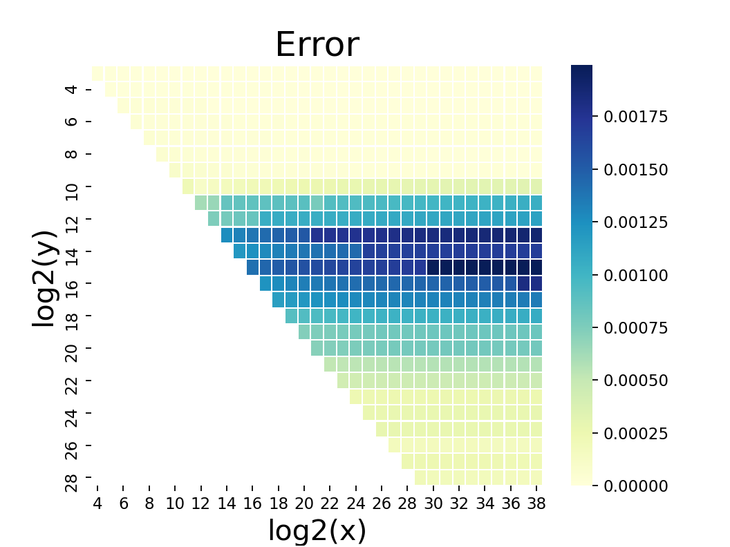 |
 | |
| (HT time)-(HT time) |
The following table is a comparison of error, time (in seconds) and Newton’s Method iterations (Its.) per algorithm and by step in the case of HT. Here :
| HT | HT | ||||||
|---|---|---|---|---|---|---|---|
| Time | Its. | Time | Its. (2) | Its. (3) | |||
| 1.004 | 0.027 | 5 | 1.014 | 0.0006 | 6 | 1 | |
| 1.031 | 0.765 | 6 | 1.034 | 0.002 | 6 | 1 | |
| 1.018 | 18.599 | 6 | 1.019 | 6.978 | 6 | 1 | |
The graphs in Figure 1 give a bit more data visually.
4 Estimating
In this section, we give advice on the best way to compute values of for various ranges of and in practice.


We considered the following algorithms to estimate , roughly ordered by how large is relative to , starting with methods that work best for small .
- •
Buchstab’s Identity, stated below, directly implies a simple recursive algorithm that gives exact values of . However, with a running time roughly proportional to the value of , it is only useful for very small inputs.
In practice, we supplement with the base case as well.
- •
Ennola’s Second Theorem was discussed in detail in §2. It is provably useful for when , but in practice we found it to be perfectly fine so long a its running time is tolerable. Precomputation requires an running time, which is quite high, but if this information is saved, then the time to compute specific values drops to a more reasonable time. It is highly accurate in practice.
- •
Algorithm HT (or HT) was discussed above in §3. This method is provably accurate for , but is a bit slow with a running time roughly linear in . Its running time is similar to Ennola’s method if precomputation is allowed, and much faster if not. Also, less extra space is required for Algorithm HT. Ennola’s method is a bit more accurate, but not provably so.
- •
Algorithm HT-fast is the version of the previous algorithm where sums of primes are estimated using the Riemann Hypothesis to bound the error. It is a bit less accurate than Algorithm HT, but much faster with a running time proportional to and the same wide range of applicability.
- •
The Dickman estimate gives
where and is the unique solution the the following equations:
Note that in the literature, one normally sees
but we find adding the second term is worthwhile in improved accuracy. This estimate is valid when , with assuming the Extended Riemann Hypothesis (ERH). Without the ERH, the lower limit on is much larger, for [13]. This method is very fast; with precomputaion of the function, evaluations of take constant time. can be computed reasonably quickly using numeric integration; see [27, 16]. It is the least accurate of the methods presented here, but its very fast computing time make it desireable, especially for large , where its accuracy is tolerable in practice.
In Figures 2 and 3 are plots indicating approximately where we recommend one uses each method to compute . They are plotted using a logarithmic scale (base 2) in both and . The key to the graphs is as follows:
![[Uncaptioned image]](2208.01725v1/indigo.png) |
Use Buchstab’s identity | ![[Uncaptioned image]](2208.01725v1/bl.png) |
Buchstab takes 1.5 seconds |
![[Uncaptioned image]](2208.01725v1/purple.png) |
Use Ennola’s Second Theorem | ![[Uncaptioned image]](2208.01725v1/pl.png) |
|
![[Uncaptioned image]](2208.01725v1/hash.PNG) |
Use HT (Ennola’s is accurate too) | ![[Uncaptioned image]](2208.01725v1/al.png) |
Ennola max (gets slow) |
![[Uncaptioned image]](2208.01725v1/aqua.png) |
Use HT (or HT) | ![[Uncaptioned image]](2208.01725v1/gl.png) |
Switch from HT to HT-Fast |
![[Uncaptioned image]](2208.01725v1/green.png) |
Use HT-Fast | ![[Uncaptioned image]](2208.01725v1/rl.png) |
|
![[Uncaptioned image]](2208.01725v1/red.png) |
Use | ![[Uncaptioned image]](2208.01725v1/kl.png) |
Methodology and Notes
- •
We implemented all the algorithms in C++, we used the standard GNU g++ compiler, and the code was run on a Linux server using standard Intel hardware.
- •
In [16] it was shown that Algorithm HT is extremely accurate in practice, and so we used either Buchstab’s algorithm, or Algorithm HT when Buchstab was too slow, as a baseline for accuracy.
- •
We collected data on the accuracy and speed of all the algorithms over the range of values shown in the graphs, except for some algorithms that got too slow.
- •
After the data was collected, we determined the ranges where each algorithm was reasonably accurate in practice.
- •
We varied the value of in the ERH cutoff for the Dickman method to see what worked best in practice.
5 Concluding Remarks
- •
- •
We currently have no theory as to why the algorithm based on Ennola’s second theorem has, in practice, applicability on a range as wide as that of Algorithm HT. It may be that a closer examination of Ennola’s proof may yield a way to improve the range.
- •
- •
In [4] it was shown how to use LMO summation to improve the running time of Algorithm HT to . It stands to reason that HT-fast can be done in time as well. As far as the authors are aware, this has not yet been implemented.
Acknowledgements
The first author was supported in part by the Butler Summer Institute (Summer 2021) and the Mathematics Research Camp (August 2021) at Butler University.
This work was presented by the first author at the Young Mathematicians Conference at The Ohio State University, August 2021, and at the Undergraduate Research Conference at Butler University, April 2022.
References
- [1] A. O. L. Atkin and D. J. Bernstein. Prime sieves using binary quadratic forms. Mathematics of Computation, 73:1023–1030, 2004.
- [2] Eric Bach and Jeffrey O. Shallit. Algorithmic Number Theory, volume 1. MIT Press, 1996.
- [3] Eric Bach and Jonathan Sorenson. An algorithm to generate random factored smooth integers, 2020. Available on arxiv.org at https://arxiv.org/abs/2006.07445.
- [4] Eric Bach and Jonathan P. Sorenson. Approximately counting semismooth integers. In Proceedings of the 38th International symposium on symbolic and algebraic computation, ISSAC ’13, pages 23–30, New York, NY, USA, 2013. ACM.
- [5] Daniel J. Bernstein. Enumerating and counting smooth integers. Chapter 2, PhD Thesis, University of California at Berkeley, May 1995.
- [6] Daniel J. Bernstein. Bounding smooth integers. In J. P. Buhler, editor, Third International Algorithmic Number Theory Symposium, pages 128–130, Portland, Oregon, June 1998. Springer. LNCS 1423.
- [7] Daniel J. Bernstein. Arbitrarily tight bounds on the distribution of smooth integers. In Bennett, Berndt, Boston, Diamond, Hildebrand, and Philipp, editors, Proceedings of the Millennial Conference on Number Theory, volume 1, pages 49–66. A. K. Peters, 2002.
- [8] J. Couveignes. Hard homogeneous spaces. 2006.
- [9] R. Crandall and C. Pomerance. Prime Numbers, a Computational Perspective. Springer, 2001.
- [10] V. Ennola. On numbers with small prime divisors. Ann. Acad. Sci. Fenn. Ser. A I, 440, 1969. 16pp.
- [11] Andrew Granville. Smooth numbers: computational number theory and beyond. In Algorithmic number theory: lattices, number fields, curves and cryptography, volume 44 of Math. Sci. Res. Inst. Publ., pages 267–323. Cambridge Univ. Press, Cambridge, 2008.
- [12] Harald Andrés Helfgott. An improved sieve of Eratosthenes. Mathematics of Computation, 89:333–350, 2020.
- [13] A. Hildebrand. On the number of positive integers and free of prime factors . Journal of Number Theory, 22:289–307, 1986.
- [14] A. Hildebrand and G. Tenenbaum. On integers free of large prime factors. Trans. AMS, 296(1):265–290, 1986.
- [15] A. Hildebrand and G. Tenenbaum. Integers without large prime factors. Journal de Théorie des Nombres de Bordeaux, 5:411–484, 1993.
- [16] Simon Hunter and Jonathan P. Sorenson. Approximating the number of integers free of large prime factors. Mathematics of Computation, 66(220):1729–1741, 1997.
- [17] D. E. Knuth and L. Trabb Pardo. Analysis of a simple factorization algorithm. Theoretical Computer Science, 3:321–348, 1976.
- [18] J. D. Lichtman and C. Pomerance. Explicit estimates for the distribution of number free of large prime factors. Journal of Number Theory, 183:1–23, 2018.
- [19] A. J. Menezes, P. C. van Oorschot, and S. A. Vanstone. Handbook of Applied Cryptography. CRC Press, Boca Raton, 1997.
- [20] Scott Parsell and Jonathan P. Sorenson. Fast bounds on the distribution of smooth numbers. In Florian Hess, Sebastian Pauli, and Michael Pohst, editors, Proceedings of the 7th International Symposium on Algorithmic Number Theory (ANTS-VII), pages 168–181, Berlin, Germany, July 2006. Springer. LNCS 4076, ISBN 3-540-36075-1.
- [21] A. Rostovtsev and A. Stoblunov. Public-key cryptosystem based on isogenies. 2006.
- [22] Jonathan P. Sorenson. A fast algorithm for approximately counting smooth numbers. In W. Bosma, editor, Proceedings of the Fourth International Algorithmic Number Theory Symposium (ANTS IV), pages 539–549, Leiden, The Netherlands, 2000. LNCS 1838.
- [23] Jonathan P. Sorenson. Two compact incremental prime sieves. LMS Journal of Computation and Mathematics, 18(1):675–683, 2015.
- [24] K. Suzuki. An estimate for the number of integers without large prime factors. Mathematics of Computation, 73:1013–1022, 2004. MR 2031422 (2005a:11142).
- [25] K. Suzuki. Approximating the number of integers without large prime factors. Mathematics of Computation, 75:1015–1024, 2006.
- [26] Gérald. Tenenbaum. Introduction to Analytic and Probabilistic Number Theory, volume 46 of Cambridge Studies in Advanced Mathematics. Cambridge University Press, english edition, 1995.
- [27] J. van de Lune and E. Wattel. On the numerical solution of a differential-difference equation arising in analytic number theory. Mathematics of Computation, 23:417–421, 1969.