Towards R-learner with Continuous Treatments

Let $\{Z_{i}=(X_{i},T_{i},Y_{i})\}_{i=1}^{n}$ be independent and identically distributed samples from the distribution of $(X,T,Y)$, where $X=(X^{(1)},\dots,X^{(d)})$ is a $d$-dimensional vector of covariates. Under Rubin’s causal model framework (Rubin 1974), $Y^{(t)}$ is the potential outcome had the unit received treatment level $T=t\in\mathbb{R}$. The causal estimand is $\tau(x,t)$ defined in (1). Due to the fundamental problem in causal inference that not all potential outcomes can be observed for a particular unit, $\tau(x,t)$ is not identifiable without further assumptions. We employ common assumptions for continuous treatments (Kennedy et al. 2017).

We summarize the notation used throughout the paper. For any vector $v$, $\|v\|$ denotes its $\ell_{2}$ norm. For any random variable $W\in\mathbb{W}$, $f(w)$ and $\mathcal{P}(w)$ denote its probability density function and probability measure. For any function $g(w)$, $P_{n}\{g(W)\}=\sum_{i=1}^{n}g(W_{i})/n$ denotes its empirical expectation and $\|g\|_{\mathcal{L}^{2}}=\{\int_{w\in\mathbb{W}}g^{2}(w)dw\}^{1/2}$, $\|g\|_{\mathcal{L}^{2}_{\mathcal{P}}}=\{\int_{w\in\mathbb{W}}g^{2}(w)d\mathcal{P}(w)\}^{1/2}$, $\|g\|_{\mathbb{W}}=\sup_{w\in\mathbb{W}}|g(w)|$ denote its $\mathcal{L}^{2}$, $\mathcal{L}^{2}_{\mathcal{P}}$ and $\mathcal{L}^{\infty}$ norms. $\mathcal{L}_{\mathcal{P}}^{2}(W)$ represents the function space of all $g(w)$ with a bounded $\mathcal{L}^{2}_{\mathcal{P}}$ norm. When $g(w)$ is a multivariate function, denote $\|g\|_{\mathbb{W}}=\sup_{w\in\mathbb{W}}\|g(w)\|$. We require two nuisance functions, the conditional outcome mean and generalized propensity score:

$\displaystyle m(x)=E(Y\mid X=x),\quad\varpi(t\mid x)=f(T=t\mid X=x).$

We denote the full conditional outcome mean model $\mu(x,t)=E(Y\mid X=x,T=t)$, and hereby define the observation noises,

$\displaystyle\varepsilon_{i}=Y_{i}-\mu(X_{i},T_{i}),\quad i=1,\dots,n,$

(2)

where $E(\varepsilon_{i}\mid X_{i},T_{i})=0$, following the definition of $\mu(x,t)$.

We first generalize the idea of the Robinson’s residual (Robinson 1988; Nie and Wager 2021) to the continuous-treatment scenario. The unconfoundedness and stable unit and treatment value imply

$\displaystyle Y_{i}^{(T_{i})}$

$\displaystyle=\mu(X_{i},T_{i})+\varepsilon_{i}=\mu(X_{i},0)+\tau(X_{i},T_{i})+\varepsilon_{i},$

(3)

where the first equality follows from Assumption 2 and equation (2), and the second equality follows from Assumption 1 and the definition of $\tau(x,t)$. Model (3) is nonparametric and free of any additional structural assumptions. Given $X_{i}$, taking the conditional expectation on (3) leads to

$\displaystyle m(X_{i})=E\big(Y^{(T_{i})}\mid X=X_{i}\big)=\mu(X_{i},0)+E_{\varpi}\{\tau(X,T)\mid X=X_{i}\},$

(4)

where the last equality is followed by the law of total expectation such that $E(\varepsilon_{i}\mid X_{i})=E\big\{E(\varepsilon_{i}\mid X_{i},T_{i})\mid X_{i}\big\}=E\big(0\mid X_{i}\big)=0.$ The notation $E_{\varpi}\{\tau(X,T)\mid X=X_{i}\}$ in (4) highlights the dependency of the conditional expectation on the generalized propensity score as $E_{\varpi}\{\tau(X,T)\mid X=X_{i}\}=\int_{t\in\mathbb{T}}\tau(X_{i},t)\varpi(t\mid X_{i})dt$. By subtracting (4) from (3) on both left- and right-hand sides, we have

$$\displaystyle Y_{i}^{(T_{i})}-m(X_{i})=\tau(X_{i},T_{i})-E_{\varpi}\{\tau(X,T)\mid X=X_{i}\}+\varepsilon_{i}.$$

(5)

By treating the left-hand side of (5) as the response and the right-hand side except $\varepsilon_{i}$ as the mean function, we derive the following population loss function,

$\displaystyle L_{c}(h)=E\big[Y-m(X)-h(X,T)+E_{\varpi}\{h(X,T)\mid X\}\big]^{2},$

(6)

which is minimized at $h=\tau$. The above derivation parallels that of the binary-treatment R-learner. In fact, a similar loss function to $L_{c}(h)$ appears in Nie and Wager 2021 under the multi-treatment setting. We view $L_{c}(h)$ as a natural generalization of the binary-treatment R-loss function (Nie and Wager 2021, $\mathsection$2) to the continuous-treatment setting, and thus refer to $L_{c}(h)$ as the generalized R-loss. In particular, under the binary-treatment case, $\tau(x,t)$ reduces to $\{\tau(x,0),\tau(x,1)\}$, where $\tau(x,0)=E(Y^{(0)}-Y^{(0)}\mid X=x)=0$ for any $x\in\mathbb{X}$, and $\tau(x,1)$ is the conditional average treatment effect of interest. It suffices to estimate $\tau(x,1)$ by solving the $h(\cdot,1)$ that minimizes (6), after imposing a zero condition of $h(\cdot,0)$:

$\displaystyle h(x,0)=0,\quad\text{for any }x\in\mathbb{X}.$

(7)

More specifically, observing that under (7) one has $h(X,T)-E_{e}\{h(X,T)\mid X\}=\{T-e(X)\}h(X,1)$ a.s., where $e(x)=\text{pr}(T=1\mid X=x)$ is the propensity score, the R-loss function (6) reduces to

$\displaystyle L_{b}(h)=E\big[Y-m(X)-\{T-e(X)\}h(X,1)\big]^{2}$

(8)

as in Nie and Wager 2021, which is also minimized at $h=\tau$.

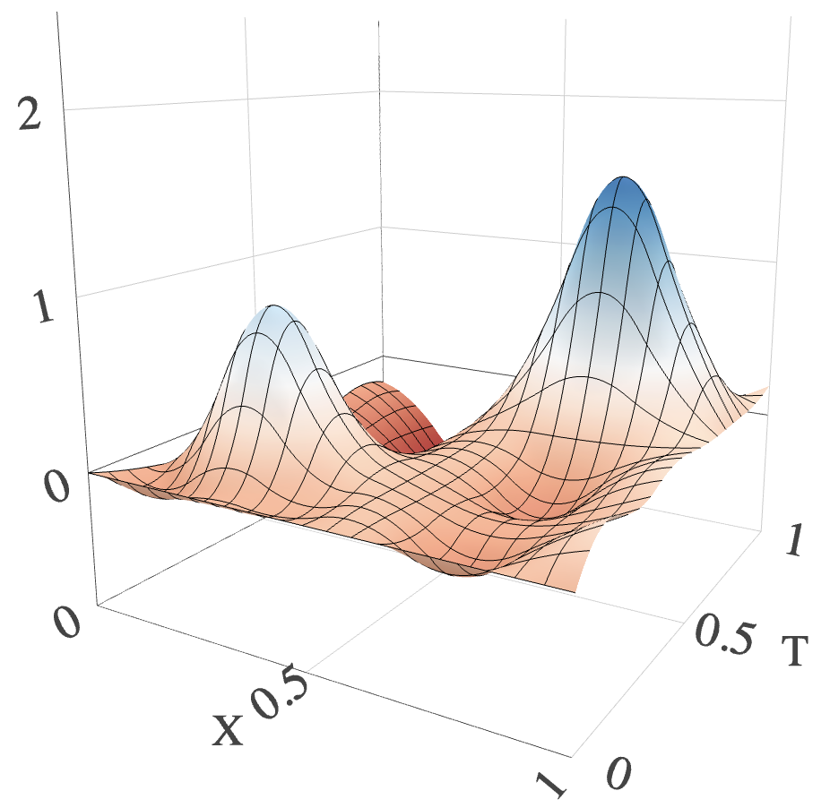
The generalization of the R-loss from the binary treatment to the continuous treatment is natural, which however results in a transition of the identifiability of $\tau(x,t)$. Suppose we construct $\hat{\tau}(x,t)$ by directly minimizing the empirical analogy of $L_{c}(\cdot)$ following Nie and Wager 2021. The R-learner for continuous treatment will have poor estimation performance, due to the non-unique identifiability of the generalized R-loss. To illustrate, we conduct a simple simulation study where we use B-splines for the nonparametric approximation of $\hat{\tau}(x,t)$. The R-learner approximates $\tau(x,t)$ well when the treatment is binary (Fig. 1a) and poorly when the treatment is continuous (Fig. 1c). The simulation details are deferred to $\mathsection$S5.

We provide a theoretical explanation for the success and failure of the identifiabilities of the R-learner for binary treatment and generalized R-learner for continuous treatment, respectively. Denote

$\displaystyle\mathcal{S}=\{h\mid h(X,T)=\tau(X,T)+s(X)\,\text{a.s., for any }s\in\mathcal{L}^{2}_{\mathcal{P}}(X)\}.$

(9)

It is easy to check that for any $h\in\mathcal{S}$,

$$Y-m(X)-[h(X,T)-E_{\varpi}\{h(X,T)\mid X\}]=Y-m(X)-[\tau(X,T)-E_{\varpi}\{\tau(X,T)\mid X\}]\quad\text{a.s.}.$$

From (6), any function $h\in\mathcal{S}$ minimizes the generalized R-loss $L_{c}(\cdot)$. Therefore, when $T$ is continuous, directly minimizing the generalized R-loss fails to uniquely identify the target estimand $\tau(x,t)$, as there are infinitely many solutions in $\mathcal{S}$. This result theoretically substantiates the ill-posedness of estimating $\tau(x,t)$ by minimizing the empirical counterpart of $L_{c}(\cdot)$ using nonparametric estimators, and also explains the failure-to-estimate issue illustrated in Fig. 1.

Part (i) of Proposition 1 below rigorously proves that $\mathcal{S}$ in fact contains all minima of $L_{c}(\cdot)$ in $\mathcal{L}_{\mathcal{P}}^{2}(X,T)$. In contrast, minimizing the binary-treatment R-loss (8) which incorporates the zero condition (7), can successfully identify $\tau$, because (7) narrows the general solution set $\mathcal{S}$ into

$\displaystyle\mathcal{S}^{\natural}=\{h\mid h(X,T)=\tau(X,T)\text{ a.s.}\}$

(10)

with a formal proof relegated to $\mathsection$S7.4 in the Supplementary Material. Despite the popular use of R-loss (8) in literature (Zhao et al. 2022; Nie and Wager 2021), the corresponding identification problem has not been rigorously discussed. Part (ii) of Proposition 1 fulfills this gap.

The contrast between Proposition 1 (i) and (ii) suggests that, in order to identify $\tau(x,t)$ nonparametrically for the continuous-treatment R-learner, it can be beneficial to leverage the zero condition (7) satisfied by $\tau(x,t)$. A straightforward way to impose the zero condition is to solve (11) among all functions satisfying (7). From a population level, one may consider to solve the following one-step optimization problem with a functional zero constraint:

$\displaystyle\argmin_{h\in\mathcal{L}_{\mathcal{P}}^{2}(X,T)\cap\{h\mid h(x,0)=0\text{ for any }x\in\mathbb{X}\}}L_{c}(h).$

(12)

However, Proposition 2 shows that, this strategy continues to fail in achieving a nonparametric identification of $\tau(x,t)$.

The failure of (12) to identify $\tau$, stems from the fundamental nature that the solutions of (11) in $\mathcal{S}$ take the form of $\tau+s$ in an almost-surely sense rather than in an exact sense. Consequently, imposing the zero condition (7) is insufficient to eliminate the solutions in $\mathcal{S}$ that manifest as $\check{\tau}(x,t\mid s)$ as long as the density function of $(X,T)$ is bounded. More specifically, any $\check{\tau}(x,t\mid s)$ can satisfy the zero condition (7) while still belong to $\mathcal{S}$. Thus the functional minima of (13) are non-unique, and the subsequent empirical nonparametric estimation procedure based on (12) still suffers severe ill-posedness due to such non-uniqueness. To be more specific, the B-spline functions satisfying the zero condition, can approximate any minimum $\check{\tau}(x,t\mid s)$ with smooth $\tau(x,t)$ and $s(x)$ arbitrarily well, as the number of basis grows; see Proposition 6(ii) for details. So for an R-learner formulated through the empirical resolution of (12) with B-spline functions, although it can satisfy the zero condition (7), it is still ill-posed. We demonstrate such ill-posedness by continuing our numerical experiment in $\mathsection$2.2. The new R-learner satisfies the zero condition yet still fails to approximate $\tau(x,t)$ well (Fig. 1d). As shown in $\mathsection$S5 in the Supplementary File, after increasing the sample size, it continuously yields poor estimation performance.

To resolve the ill-posedness of nonparametrically estimating $\tau(x,t)$ through the one-step R-loss optimization (12), it is necessary to address the non-uniqueness of the optimization solutions. Tikhonov $\ell_{2}$-regularization (Tikhonov 1963), originally developed in non-linear functional analysis, aims to identify a specific solution for the functional least-squares problems with non-unique solutions (Zeidler 2013, $\mathsection$37.14). Tikhonov regularization, together with the idea of the functional zero constraint in $\mathsection$2.3, inspires our two-step identification strategy for $\tau(x,t)$.

In Step I, from the population level, we solve the $\ell_{2}$-regularized variant of (11) with some given $\rho>0$,

$\displaystyle{\tau}_{\rho}=\argmin_{h\in\mathcal{L}_{\mathcal{P}}^{2}(X,T)}L_{c,\ell_{2}}(h\mid\rho)$

$\displaystyle=\argmin_{h\in\mathcal{L}_{\mathcal{P}}^{2}(X,T)}L_{c}(h)+\rho\|h\|_{\mathcal{L}_{\mathcal{P}}^{2}}^{2}.$

(14)

The new loss $L_{c,\ell_{2}}(h\mid\rho)$ is strictly convex over $\mathcal{L}_{\mathcal{P}}^{2}(X,T)$ due to the addition of a strictly convex functional $\rho\|h\|_{\mathcal{L}^{2}_{\mathcal{P}}}^{2}=\rho E\{h^{2}(X,T)\}$. Thus minimizing $L_{c,\ell_{2}}(h\mid\rho)$ becomes well-posed and yields a unique functional minimum ${\tau}_{\rho}$. Theorem 1 explicitly characterizes this unique minimum.

Theorem 1 implies that we can identify an intermediary function in $\mathcal{S}$, namely, $\tilde{\tau}$ in (15), by augmenting $\tau_{\rho}$ with a factor of $(1+\rho)$, i.e., $\tilde{\tau}=(1+\rho)\tau_{\rho}$. The $\tilde{\tau}$ is a solution for the original R-loss $L_{c}(h)$. We defer a more detailed discussion on the intuition behind why minimizing the $\ell_{2}$-regularized R-loss helps to identify this specific solution $\tilde{\tau}$ for the original R-loss, to Section S1 in the Supplementary File.

In Step II, we transform $\tilde{\tau}$ through a zero-constraining operator $\mathscr{C}(\cdot):\mathcal{L}_{\mathcal{P}}^{2}(X,T)\mapsto\mathcal{L}_{\mathcal{P}}^{2}(X,T)$ such that $\mathscr{C}(h)(x,t)=h(x,t)-h(x,0)$ for any $h\in\mathcal{L}_{\mathcal{P}}^{2}(X,T)$. Then we have

$$\mathscr{C}(\tilde{\tau})(x,t)=\mathscr{C}((1+\rho)\tau_{\rho})(x,t)=(1+\rho)\left\{{\tau}_{\rho}(x,t)-{\tau}_{\rho}(x,0)\right\}.$$

The operator $\mathscr{C}(\cdot)$ ensures that any function undergoing its transformation will satisfy the zero condition (7). Because ${\tau}$ is the only function in $\mathcal{S}$ that satisfies the zero condition (7), transforming any function in the solution set $\mathcal{S}$ will indeed identify $\tau$. Thus with $\tilde{\tau}\in\mathcal{S}$, $\mathscr{C}(\tilde{\tau})$ in our second step ultimately identifies $\tau$. Formally, we have the following theoretical justification.

Our two-step identification strategy for $\tau(x,t)$ based on Tikhonov $\ell_{2}$-regularization, differs from the classical expectation-based identification approach, where the causal estimand is identified by the expectation of a specific estimating function, and the estimator is the empirical average of that function; see e.g., the augmented inverse propensity score weighting estimator for average treatment effect (Robins et al. 1994), or the debiased estimator for a general estimand (Chernozhukov et al. 2023). Our two-step identification relies on a sequence of functionals indexed by $\rho$, and any fixed and positive $\rho$ with $n$ is sufficient to develop a well-posed empirical R-learner. On the other hand, a fast vanishing $\rho$ will introduce large estimation variance. Intuitively, a small $\rho$ will result in a weak $\ell_{2}$-regularization. Then with finite samples, such weak $\ell_{2}$-regularization can not make the minimization of the empirical analogy of $L_{c,\ell_{2}}(h\mid\rho)$ significantly different from naively minimizing the empirical analogy of $L_{c}(h)$, which is ill-posed as shown in $\mathsection$2.2. Such phenomenon will also be revealed by Theorem 3, where a fast vanishing $\rho$ cannot yield a well-controlled error rate of our proposed estimator, while a fixed $\rho>0$ could.

Our identification strategy leads to an $\ell_{2}$-regularized R-learning procedure, briefly, the $\ell_{2}$-regularized R-learner. Formal algorithm and implementation details of $\ell_{2}$-regularized R-learner are deferred to $\mathsection$S1 in Supplementary File. The newly proposed R-learner inherits many practical and theoretical advantages from the original R-learner (Nie and Wager 2021). Practically, minimizing the empirical analogy of $L_{c,\ell_{2}}(h\mid\rho)$ separates the process of estimating the nuisance functions and that of estimating the target estimand, both of which can be implemented by flexible machine learning methods. Theoretically, when $\tau(x,t)$ is approximated by the method of sieve, our proposed R-learner is theoretically robust to slow convergence rates of the nuisance estimators. Notably, this paper mainly implements our $\ell_{2}$-regularized R-learner with the method of sieve for our asymptotical and numerical analysis. Nevertheless, our estimation strategy and general Algorithm 1 are not tied on the method of sieve. In fact, any loss-minimization method, e.g., the regularized nonparametric regression, deep neural networks, and boosting can be flexibly used to specify $\mathcal{H}$ and minimize (S2) in Algorithm 1, for $\tau(x,t)$ estimation. For future research, it is interesting to explore the practical and theoretical performances of the $\ell_{2}$-regularized R-learner, implemented with other machine learning algorithms for $\tau(x,t)$ approximation.

Continuing with the numerical experiment in $\mathsection$2.2, we demonstrate the effectiveness of the proposed $\ell_{2}$-regularized R-learner (Fig. 1e), which well approximates the true $\tau(x,t)$ (Fig. 1b). We further generalize the S-learner and X-learner proposed in Künzel et al. 2019 into the continuous-treatment case, with details introduced in $\mathsection$S4. The $\tau(x,t)$ estimators by the generalized S- and X-learners for the numerical experiment in $\mathsection$2.2, are reported in Fig. S2, and we can see our proposed R-learner also outperforms these two generalized meta-learners.

References

- Aizerman et al. (1964) Aizerman, M. A., E. M. Braverman, and L. I. Rozonoer (1964). Theoretical foundation of potential functions method in pattern recognition. Avtomat. i Telemekh. 25(6), 917–936.
- Belloni et al. (2019) Belloni, A., V. Chernozhukov, D. Chetverikov, and I. Fernández-Val (2019). Conditional quantile processes based on series or many regressors. J. Econom. 213(1), 4–29.
- Belloni et al. (2015) Belloni, A., V. Chernozhukov, D. Chetverikov, and K. Kato (2015). Some new asymptotic theory for least squares series: Pointwise and uniform results. J. Econom. 186(2), 345–366.
- Bhatia (2013) Bhatia, R. (2013). Matrix Analysis, Volume 169. Springer Science & Business Media.
- Cai and Zhang (2018) Cai, T. T. and A. Zhang (2018). Rate-optimal perturbation bounds for singular subspaces with applications to high-dimensional statistics. Ann. Stat. 46(1), 60–89.
- Chen (2007) Chen, X. (2007). Large sample sieve estimation of semi-nonparametric models. Handbook of Econometrics 6, 5549–5632.
- Chen and Christensen (2015) Chen, X. and T. M. Christensen (2015). Optimal uniform convergence rates and asymptotic normality for series estimators under weak dependence and weak conditions. J. Econom. 188(2), 447–465.
- Chernozhukov et al. (2018) Chernozhukov, V., D. Chetverikov, M. Demirer, E. Duflo, C. Hansen, W. Newey, and J. Robins (2018). Double/debiased machine learning for treatment and structural parameters: Double/debiased machine learning. Econom. J. 21(1), C1–C68.
- Chernozhukov et al. (2023) Chernozhukov, V., W. K. Newey, and R. Singh (2023). A simple and general debiased machine learning theorem with finite-sample guarantees. Biometrika 110(1), 257–264.
- Cui et al. (2020) Cui, Y., H. Pu, X. Shi, W. Miao, and E. T. Tchetgen (2020). Semiparametric proximal causal inference. arXiv:2011.08411.
- Davis and Kahan (1970) Davis, C. and W. M. Kahan (1970). The rotation of eigenvectors by a perturbation. iii. SIAM J. Numer. Anal. 7(1), 1–46.
- Douglas et al. (1975) Douglas, J., T. Dupont, and L. Wahlbin (1975). Optimal error estimates for galerkin approximations to solutions of two-point boundary value problems. Math. Comput. 29(130), 475–483.
- Eckart and Young (1936) Eckart, C. and G. Young (1936). The approximation of one matrix by another of lower rank. Psychometrika 1(3), 211–218.
- Geman and Hwang (1982) Geman, S. and C.-R. Hwang (1982). Nonparametric maximum likelihood estimation by the method of sieves. Ann. Stat. 10, 401–414.
- Golub et al. (1979) Golub, G. H., M. Heath, and G. Wahba (1979). Generalized cross-validation as a method for choosing a good ridge parameter. Technometrics 21(2), 215–223.
- Golub and Van Loan (2013) Golub, G. H. and C. F. Van Loan (2013). Matrix Computations, Volume 3. JHU Press.
- Hansen (2014) Hansen, B. E. (2014). Nonparametric sieve regression: Least squares, averaging least squares, and cross-validation. Handbook of Applied Nonparametric and Semiparametric Econometrics and Statistics, 215–248.
- Hill (2011) Hill, J. L. (2011). Bayesian nonparametric modeling for causal inference. J. Comput. Graph. Stat. 20(1), 217–240.
- Hoerl and Kennard (1970) Hoerl, A. E. and R. W. Kennard (1970). Ridge regression: Biased estimation for nonorthogonal problems. Technometrics 12(1), 55–67.
- Horn and Johnson (1991) Horn, R. A. and C. R. Johnson (1991). Topics in Matrix Analysis. Cambridge University Press.
- Huang et al. (2003) Huang, J. Z. et al. (2003). Local asymptotics for polynomial spline regression. Ann. Stat. 31(5), 1600–1635.
- Ichimura and Todd (2007) Ichimura, H. and P. E. Todd (2007). Implementing nonparametric and semiparametric estimators. Handb. Econom. 6, 5369–5468.
- Kennedy (2023) Kennedy, E. H. (2023). Towards optimal doubly robust estimation of heterogeneous causal effects. Electron. J. Stat. 17(2), 3008–3049.
- Kennedy et al. (2020) Kennedy, E. H., S. Balakrishnan, and M. G’Sell (2020). Sharp instruments for classifying compliers and generalizing causal effects. Ann. Stat. 48(4), 2008–2030.
- Kennedy et al. (2017) Kennedy, E. H., Z. Ma, M. D. McHugh, and D. S. Small (2017). Non-parametric methods for doubly robust estimation of continuous treatment effects. J. R. Stat. Soc. Ser. B 79(4), 1229–1245.
- Kunoth et al. (2018) Kunoth, A., T. Lyche, G. Sangalli, and S. Serra-Capizzano (2018). Splines and PDEs: from Approximation Theory to Numerical Linear Algebra. Springer.
- Künzel et al. (2019) Künzel, S. R., J. S. Sekhon, P. J. Bickel, and B. Yu (2019). Metalearners for estimating heterogeneous treatment effects using machine learning. Proc. Natl. Acad. Sci. U.S.A. 116(10), 4156–4165.
- Newey (1997) Newey, W. K. (1997). Convergence rates and asymptotic normality for series estimators. J. Econom. 79(1), 147–168.
- Neyman (1990) Neyman, J. (1923/1990). On the application of probability theory to agricultural experiments. Statist. Sci. 5, 465–472. Essay on principles. Section 9. Translated by Dabrowska, D.M. and Speed, T.P.
- Nie and Wager (2021) Nie, X. and S. Wager (2021). Quasi-oracle estimation of heterogeneous treatment effects. Biometrika 108(2), 299–319.
- O’Sullivan (1986) O’Sullivan, F. (1986). A statistical perspective on ill-posed inverse problems. Statist. Sci. 1, 502–518.
- Robins (1994) Robins, J. M. (1994). Correcting for non-compliance in randomized trials using structural nested mean models. Commun. Stat. - Theory Methods 23(8), 2379–2412.
- Robins et al. (1994) Robins, J. M., A. Rotnitzky, and L. P. Zhao (1994). Estimation of regression coefficients when some regressors are not always observed. J. Am. Stat. Assoc. 89(427), 846–866.
- Robinson (1988) Robinson, P. M. (1988). Root-n-consistent semiparametric regression. Econometrica 56, 931–954.
- Rubin (1974) Rubin, D. B. (1974). Estimating causal effects of treatments in randomized and nonrandomized studies. J. Educ. Psychol. 66(5), 688.
- Rudelson (1999) Rudelson, M. (1999). Random vectors in the isotropic position. J. Funct. Anal. 164(1), 60–72.
- Rudin (1991) Rudin, W. (1991). Functional Analysis. McGraw-Hill Science/Engineering/Math.
- Schacke (2004) Schacke, K. (2004). On the kronecker product. Master’s thesis, University of Waterloo.
- Schick (1986) Schick, A. (1986). On asymptotically efficient estimation in semiparametric models. Ann. Stat., 1139–1151.
- Shalit et al. (2017) Shalit, U., F. D. Johansson, and D. Sontag (2017). Estimating individual treatment effect: generalization bounds and algorithms. In Proc. 34th Int. Conf. Mach. Learn. (ICML 2017), pp. 3076–3085. PMLR.
- Shi et al. (2022) Shi, C., S. Zhang, W. Lu, and R. Song (2022). Statistical inference of the value function for reinforcement learning in infinite-horizon settings. J. R. Stat. Soc. Ser. B 84(3), 765–793.
- Tikhonov (1963) Tikhonov, A. N. (1963). On the solution of ill-posed problems and the method of regularization. In Doklady Akademii Nauk, Volume 151, pp. 501–504. Russian Academy of Sciences.
- Tikhonov et al. (1995) Tikhonov, A. N., A. Goncharsky, V. Stepanov, and A. G. Yagola (1995). Numerical Methods for the Solution of Ill-posed Problems, Volume 328. Springer Science & Business Media.
- Van der Laan et al. (2007) Van der Laan, M. J., E. C. Polley, and A. E. Hubbard (2007). Super learner. Stat. Appl. Genet. Mol. Biol. 6(1).
- Wager and Athey (2018) Wager, S. and S. Athey (2018). Estimation and inference of heterogeneous treatment effects using random forests. J. Am. Stat. Assoc. 113(523), 1228–1242.
- Wasserman (2004) Wasserman, L. (2004). All of Statistics: a Concise Course in Statistical Inference, Volume 26. Springer.
- Wasserman (2006) Wasserman, L. (2006). All of Nonparametric Statistics. Springer Science & Business Media.
- Weyl (1912) Weyl, H. (1912). Das asymptotische verteilungsgesetz der eigenwerte linearer partieller differentialgleichungen (mit einer anwendung auf die theorie der hohlraumstrahlung). Math. Ann. 71(4), 441–479.
- Yadlowsky et al. (2018) Yadlowsky, S., H. Namkoong, S. Basu, J. Duchi, and L. Tian (2018). Bounds on the conditional and average treatment effect with unobserved confounding factors. arXiv:1808.09521.
- Zeidler (2013) Zeidler, E. (2013). Nonlinear Functional Analysis and Its Applications: III: Variational Methods and Optimization. Springer Science & Business Media.
- Zhao et al. (2022) Zhao, Q., D. S. Small, and A. Ertefaie (2022). Selective inference for effect modification via the lasso. J. R. Stat. Soc. Ser. B 84(2), 382–413.
Supplementary material for “Towards R-learner with Continuous Treatments”
Supplementary material includes formal algorithms and implementation details of the proposed -regularized R-learner, general asymptotic results, generalized S- and X-learners with continuous treatments, a cross-validation-based tuning parameter selection method, details of all numerical experiments, an introduction to B-splines, and all technical proofs.
S1 -regularized R-learner: Formal algorithm and more discussions
In this section, we introduce the general -regularized R-learner in details, developed based on the identification strategy described in Section 2.4. Let denote the function class used to approximate , which can be implemented using various machine learning algorithms, such as linear regression, random forests, or neural networks.
To approximate the population loss