WIMP and FIMP Dark Matter in Singlet-Triplet Fermionic Model Preprint: IP/BBSR/2022-05
Abstract
We present an extension of the SM involving three triplet fermions, one triplet scalar and one singlet fermion, which can explain both neutrino masses and dark matter. One triplet of fermions and the singlet are odd under a symmetry, thus the model features two possible dark matter candidates. The two remaining -even triplet fermions can reproduce the neutrino masses and oscillation parameters consistent with observations. We consider the case where the singlet has feeble couplings while the triplet is weakly interacting and investigate the different possibilities for reproducing the observed dark matter relic density. This includes production of the triplet WIMP from freeze-out and from decay of the singlet as well as freeze-in production of the singlet from decay of particles that belong to the thermal bath or are thermally decoupled. While freeze-in production is usually dominated by decay processes, we also show cases where the annihilation of bath particles give substantial contribution to the final relic density. This occurs when the new scalars are below the TeV scale, thus in the reach of the LHC. The next-to-lightest odd particle can be long-lived and can alter the successful BBN predictions for the abundance of light elements, these constraints are relevant in both the scenarios where the singlet or the triplet are the long-lived particle.In the case where the triplet is the DM, the model is subject to constraints from ongoing direct, indirect and collider experiments. When the singlet is the DM, the triplet which is the next-to-lightest odd particle can be long-lived and can be probed at the proposed MATHUSLA detector. Finally we also address the detection prospects of triplet fermions and scalars at the LHC.
1 Introduction
Numerous cosmological and astrophysical observations indicate that of the energy budget of the universe is in the form of dark matter (DM). However, we are still in the dark about the nature and the origin of the dark matter. The absence of a DM candidate within the Standard Model (SM) gives compelling evidence for physics beyond the Standard Model (BSM). Weakly Interacting Massive Particles (WIMP) have been the leading candidate for DM for decades. WIMPs have a mass around the electroweak scale and interact with constituents of the plasma in the early Universe via electroweak interactions. WIMPs decouple from the thermal bath through the freeze-out mechanism and can naturally explain the DM relic density extracted from precise measurements of the Cosmic Microwave Background Ade:2015xua. However the null results from various direct and indirect searches for WIMP DM motivate the exploration of alternative DM production mechanisms. The production of DM through the thermal freeze-in mechanism Hall:2009bx is one of the most popular alternatives. This mechanism involves a Feebly Interacting Massive Particle (FIMP) which interacts so feebly that it never attains chemical equilibrium with the thermal bath. The DM is produced through decay and/or annihilations of SM and BSM particles which are in equilibrium with the thermal plasma. Another possibility is to have DM produced at a late epoch of the Universe through the out-of-equilibrium decay of particles that have themselves frozen-in or frozen-out. The latter is known as the superWIMP mechanism Feng:2003xh.
In addition to the DM problem, the SM fails to address the issue of neutrino masses and mixings for which their exist strong experimental evidence. One of the most promising model to explain the neutrino masses relies on an extension of the SM with fermion triplets that generate the active neutrino masses through the Type-III seesaw mechanism Foot:1988aq. In order to incorporate a DM candidate, this model can further be extended with a dark sector comprising a fermion triplet having gauge interaction with SM states and a gauge singlet fermionic state . The dark sector is odd under a symmetry which ensures that either of the neutral components or is stable depending on their masses and can thus be a good dark matter candidate. In addition, this model also contains a scalar triplet () having zero hypercharge. Electroweak symmetry breaking (EWSB) induces a vev for the neutral component of , this vev then generates a mixing between and N. The neutrino singlet-triplet fermionic model (STFM) can thus explain neutrino masses while providing a DM candidate that can either be the singlet or the triplet.
The properties of WIMP DM in the singlet-triplet fermionic model were studied in Choubey:2017yyn; Chardonnet:1993wd. It was shown that the presence of the additional state in the dark sector impacts significantly the phenomenology as compared with scenarios with only a singlet or a triplet of fermions in the dark sector. In this article we explore further avenues for DM formation in the STFM model and entertain the possibility that the singlet state in the dark sector is feebly interacting. This requires that the Yukawa coupling between the singlet and triplet dark states and the triplet scalar be feeble. Under these conditions, DM can be either a FIMP, when the singlet is lightest, or a WIMP, when the triplet is lightest. In this model, several mechanisms can contribute to DM formation. The WIMP can be produced through the freeze-out mechanism and through the decay of the heavier FIMP in the dark sector, we refer to the latter as non-thermal freeze-in production. When the singlet FIMP is the lightest state, it can be produced through the decay or scattering of any SM or BSM particle in the thermal bath, this is thermal freeze-in production, or can also receive a contribution from the out-of-equilibrium decay of the heavier WIMP produced through freeze-out, also called non-thermal freeze-in production.
To explore all possibilities for DM formation we consider two scenarios. In the first scenario, is the DM candidate and N is the next-to-lightest odd particle (NLOP). In the minimal DM model with only a fermion triplet, it was shown that the triplet is required to be rather heavy, Cirelli:2005uq to have a large enough relic abundance. Indeed the thermally averaged cross section increases as the mass of the decreases, thus for lower values of the relic density of is below the observed value. The presence of the singlet NLOP can change this conclusion. The NLOP which never attains thermal and chemical equilibrium with bath particles can be produced through the freeze-in mechanism and at late times decay into , thus increasing the relic density of .
In the second scenario, N is the lightest dark sector particle and the DM candidate while is the NLOP. The production of through the freeze-in mechanism is directly proportional to the dark sector Yukawa coupling , for large enough coupling this can be sufficient to reproduce the DM relic density. When the Yukawa coupling is small N can also be produced through out-of-equilibrium decay of . For this to be efficient the abundance of must be large enough, which requires . In both scenarios the production of the FIMP can arise from decays or from scattering of particles in the thermal bath, an important contribution from annihilation processes however requires that the new scalar fields be rather light, at the TeV scale or below. In this context, the discovery prospects of scalar triplets () at the LHC are improved.
The late decay of the heavier state in the dark sector for the two scenarios considered can disrupt the successful predictions of big bang nucleosynthesis (BBN). In particular, constraints from hadronic energy injection become important when the lifetime of the late decaying particle exceeds 100 sec. The impact of these constraints on the model parameters is elaborately discussed. Moreover when the triplet is long-lived, the charged component can be searched for at the LHC through its disappearing track signature.
The manuscript is organised as follows. The model is described in Section 2. In Section 3 and 4, we discuss theoretical constraints on the scalar sector as well as constraints on DM from astrophysical, cosmological and collider observables. Section 5 contains most of our results, dark matter production is explored in detail for the two scenarios considered and a subsection is dedicated to the case where the BSM scalar sector is light. Moreover the impact of BBN constraints arising from the late production of DM through out-of-equilibrium decay is investigated. The prospects for searches for triplet fermions and triplet scalars at the LHC are presented in Section 6. We present our conclusions in Section 7. Necessary calculational details are provided in the Appendix A.
2 The Model
In addition to the SM fields, the STFM model contains triplet fermions , a SM gauge singlet fermion and a triplet scalar field . We show the particle content of the model in Table. 1. The Lagrangian possesses a discrete symmetry, in addition to the SM gauge symmetries. The latter is required to stabilise the DM fields. The SM fields, the scalar triplet and two of the fermionic triplets are even under this symmetry while one of the fermionic triplet are odd under the symmetry and form the dark sector. The Lagrangian reads,
|
|
|
| ||||||||||||||||||||||||||||||||||||||||||||||||||||||||||||||||||||||||
where the triplet fermion takes the following form,
| (2) |
The triplet scalar field is represented as
| (3) |
where is a single real field and and are charge conjugate to each other. Note that does not include the potential for the standard Higgs field . With and , the scalar potential of the model has the following form,
| (4) | |||||
In general, a term is also allowed by the gauge symmetry, however, this term can be decomposed into two terms which are similar to the quartic coupling associated with and . Hence, we do not include this term in the Lagrangian. The quadratic and quartic couplings associated with the potential obey the following conditions,
| (5) |
The neutral real component of acquires a vacuum expectation value, , and breaks the electroweak symmetry. The field acquires an induced vev , which obeys the following relation,
| (6) |
Note that, for or the electroweak vev , the vev of will also vanish. Hence, the vev depends heavily on the electroweak vev. We expand the fields and as follows,
| (7) |
2.1 Neutral and charged scalar masses and mixings
After symmetry breaking, the mass matrix for the CP even neutral Higgs in the basis and has the following form,
| (8) |
The above mass matrix can be diagonalised by a unitary matrix and the mass basis fields , are related to the fields , in the following way,
| (9) |
where is the mixing angle between the neutral scalar fields. We denote the masses of by , respectively,
The fields of the SM Higgs doublet is “eaten” by the SM gauge boson and the gauge boson acquires mass. The charged scalars and also mix and one becomes the Goldstone boson “eaten” by . The physical charged scalar fields are related to the fields and in the following way,
| (11) |
where is the mixing angle and depends on the ratio of the vevs of the doublet and triplet,
| (12) |
In the above is the charged Goldstone and is the physical charged scalar field with mass ,
| (13) |
In the following we will use the masses, mixing angles and vevs as fundamental parameters, the quadratic and quartic couplings can be expressed in terms of these as,
| (14) |
Once the SM Higgs doublet and the triplet Higgs acquired vevs, then the W-boson mass and Z-boson mass take the following form,
| (15) |
The extra vev shifts the electroweak precision parameter as follows,
| (16) |
Note that the vev of the Higgs triplet is constrained by precision electroweak data. Recent results from a global fit to the SM lead to ParticleDataGroup:2020ssz. From this, a upper bound GeV can be derived. The improvement over the previous bound Erler:2004nh; Erler:2008ek on is due partly to a more precise determination of . However, if we rescale using the W-boson mass announced by the CDF-II collaboration CDF:2022hxs then the bound on the vev is relaxed to GeV. In our scans we will take even a wider range to allow for potential BSM effects in the electroweak precision fit, namely we consider GeV, which is obtained using of Erler:2004nh; Erler:2008ek while neglecting the scalar loop contributionsChen:2008jg. Note however that the DM analysis that we perform is mostly independent of the choice of .
2.2 Dark Matter Mass
The two neutral fermionic states and mix and the mixing term is proportional to . The mass matrix for the neutral fermions has the following form,
| (17) |
and the mass eigenstates and weak eigenstates are related as follows:
| (18) |
Diagonalising Eq. (17), the tree level mass eigenstates can be expressed as,
where the mixing angle is
| (20) |
The Yukawa coupling can further be expressed in terms of and ,
| (21) |
where . In Eq. (), is the Yukawa term which relates the fermionic triplet with the fermionic singlet. Here we are exploring the regime where the coupling is feeble , . Hence, the mixing angle is heavily suppressed, and the masses of and simplify to
| (22) |
The state and therefore primarily consist of the singlet and triplet fermions, respectively with a very tiny admixture. In this paper, we consider both scenarios, where either or is the DM, with a basic difference that is a WIMP DM and is a FIMP DM particle.
2.3 Neutrino Mass
The state is the DM candidate and does not participate in neutrino mass generation. However, the other two states mix with active neutrinos and generate light neutrino masses via the seesaw mechanism. Since only two triplet fermions participate in neutrino mass generation, hence, the Dirac mass term has the following form,
| (23) |
We consider a basis of where the mass matrix of neutral triplet fermion is diagonal,
| (24) |
The light neutrino mass has the following expression,
| (25) |
where represents the mass matrix for active light neutrinos, . We denote the physical masses of by , which has the following form,
| (26) |
Note that if we consider all the elements of and matrices as real then we have eight independent variables. The constraints from measurements of the oscillation parameters impose five conditions on the neutrino masses and mixings namely three mixing angles , , and two mass square differences , . Moreover, there is a bound the sum of the light neutrino masses from cosmology, eV Ade:2015xua. Since the neutrino sector contains eight variables and six constraints, the latter can easily be satisfied. The mass of the triplet fermion is constrained from LHC searches as GeV ATLAS:2022yhd. This LHC search is based on the multi lepton searches from the decay of produced via electroweak gauge bosons. When the collider bound is satisifed it is straightforward to obtain eV scale neutrino mass, for example for TeV one needs GeV. We refrain from further detailed analysis on the neutrino mass as this does not have any effect on the DM phenomenology that we study in the following. The free parameters of the model relevant to the dark sector and in particular for obtaining the DM relic density are taken as,
| (27) |
3 Constraints on the scalar sector
In this section, we briefly discuss the theoretical constraints which are relevant in our analysis of the scalar sector. Specifically, we consider the bounds which arise in order to keep the quartic couplings of the scalar potential in the perturbative regime. The choice of quartic couplings, scalar masses and mixings heavily influence our subsequent analysis of DM production, since in this work DM production significantly depends on the choice of BSM Higgs mass.


As discussed before, and are the two mixing angles in the scalar sector, being the neutral BSM Higgs mixing and is the charged Higgs mixing angle. In Fig. (1), we show scatter plots in the and planes after demanding the quartic couplings to be in the perturbative regime and positive . From the left panel(LP), where we consider random values for the masses of the BSM Higgs states i.e., , , it is evident that there is a sharp correlation between and and that they can not be chosen arbitrarily. Throughout our analysis, we consider to be consistent with the perturbative constraint. In the right panel(RP), we show the scatter plot in the plane where the variation in the color bar represents the charged Higgs mixing angle . We can see that for higher values of a large mass gap is disallowed in order to keep the quartic coupling in the perturbative regime. In our analysis we have considered these bounds on the masses of and , and throughout the paper we set degenerate masses for the charged and neutral Higgs i.e., . Note that it would be possible to relax our assumptions and consider for the lower mass range of , however is not a crucial parameter for DM observables thus it would not affect our conclusions.
There are a number of experimental constraints which are applicable on the neutral and charged BSM Higgs masses and , as well as on the mixing angle between CP even neutral Higgs. We discuss these constraints in detail in Section. 6. We have specifically considered these following searches
- •
Higgs signal strength measurements from TeV LHC searches ATLAS:2020qdt
- •
Higgs to di-photon ATLAS:2018hxb
- •
BSM Higgs search via ATLAS:2020tlo, ATLAS:2020fry
The choice of model parameters that we consider for the DM analysis is consistent with these experimental searches.
4 DM Constraints
In this work, we consider scenarios where either the WIMP () or the FIMP () forms DM. Hence, depending on our choice, different constraints apply on the DM and on the next to lightest odd particle (NLOP).
4.1 DM relic density
The DM relic density has been determined precisely by PLANCK measurements of the CMB Ade:2015xua,
| (28) |
We will in general impose this bound from the relic density on our scenarios, one exception is in section 5.3 where we allow for DM to be over-abundant hence consider a larger range. The predictions for the relic density for the different DM production mechanisms in the STFM will be discussed in detail in Section 5.
4.2 Collider constraints on
Collider constraints on apply irrespectively of our choice of a thermal/non-thermal DM. The charged component of the triplet, is nearly degenerate with the neutral component, with a maximum mass splitting of 167 MeV Cirelli:2005uq. Thus the charged triplet fermion state is long-lived and constrained from LHC disappearing track searches. The charged particle decays to the neutral particle and charged pion () and the is very difficult to reconstruct due to its small momentum. Therefore, inside the detector, the decay of the charged particle manifest itself as a disappearing track. In Fig. 2, we show the constraints in the plane - (the lifetime) as obtained from ATLAS ATLAS:2017oal; ATLAS:2022rme and CMSCMS:2018rea searches on disappearing tracks. In this figure, the green solid line represents the prediction for the lifetime of in the STFM. This figure shows clearly that GeV is ruled out by ATLAS search with , which in turn means that the neutral triplet fermion is also ruled out when GeV. The light green dotted line represents the projection for HL-LHC, taken from Dainese:2019rgk.


4.3 DM direct and indirect detection
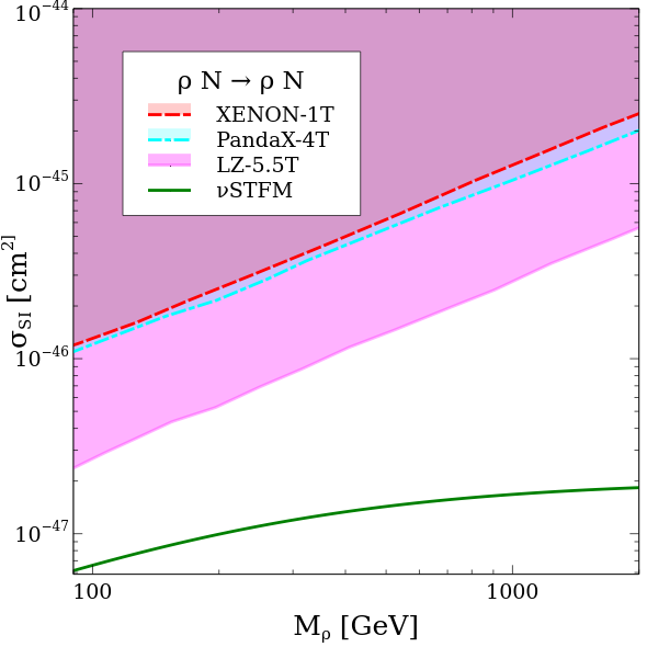
The direct and indirect detection constraints are only relevant for WIMP DM, that is when is the DM. For a FIMP DM the suppressed interactions with SM particles entail that these constraints do not play a role in our model.11 1 Direct detection can constrain FIMPs in the presence of a very light mediator Hambye:2018dpi; Belanger:2020npe, this is not the case here as all mediators are in the range TeV. In Fig. 3, we show bounds on the mass of DM, , and its spin independent/annihilation cross-sections that determine the direct detection rate. In the STFM there is no tree-level process for DM elastic scattering on nucleons but the process can happen at one loop through the diagram mediated by . The spin-independent cross-section, , for (where N is nucleon) direct detection process is given analytically by Hisano:2011cs,
| (29) |
where ( is the nucleon mass) and depends on the DM interaction with the nucleons and the nuclear form factors which are discussed in detail in Hisano:2011cs. In the DD cross section we have also taken into account the two loop gluonic which suppress the direct detection cross section as discussed in Hisano:2011cs. Note that including only the quark contributionsCirelli:2005uq, overestimates the spin independent cross section as the quark and gluon contributions cancel against each other. Fig. 3 shows that the theoretical prediction for (green) is lower than the experimental upper limit from Xenon-1T (red) XENON:2018voc, PandaX-4T (cyan) Liu:2022zgu and LUX-ZEPLIN (magenta) LUX-ZEPLIN:2022qhg. Therefore, in STFM, we do not have any bound on the DM mass from the DD experiments.
DM can also be detected indirectly by observing gamma-rays originating from DM annihilation in galaxies. In particular, in the STFM DM annihilates to via a t-channel process mediated by the charged fermion . The predicted cross-section, is compared with the upper limit on the same cross-section obtained from analysing data from Dwarf Spheroidal Galaxies from the satellite-based Fermi-LAT and earth-based MAGIC collaborations MAGIC:2016xys; Reinert:2017aga. In the right panel of In Fig. 3, we see that this leads to a constraint on the DM mass GeV. This is rather weak as compared to the direct detection constraint. In this work to analyse the thermal DM scenario, we have mostly considered DM masses in the range of 700 GeV to 1500 GeV which are safe from all kinds of bounds and can be probed by the collider experiment HL-LHC. Note that in the mass range above 1500 GeV, DM annihilation will get Sommerfeld enhancement Hisano:2003ec; Hisano:2004ds and can be in tension with the bound coming from DM indirect detection experiments.
4.4 BBN constraints
The primordial elements nucleosynthesis occurs approximately between 1 and seconds. The long lived particle decaying after 1 sec can inject sufficient energy to the thermal plasma and perturb the primordial light elements either through hadro-dissociation, interconversion or photo dissociation. In our analysis, the NLOP can decay to DM after 1 sec depending upon the coupling strength . The decay of NLOP also injects hadronic energy to the thermal plasma which disrupts the formation of light elements during BBN. The BBN constraint on the amount of hadronic energy released through late decay of long lived decaying particles were derived in Kawasaki:2017bqm. The hadronic energy released through late decay of NLOP is given by,
| (30) |
where is the hadronic branching fraction that is approximately be given by,
| (31) |
is the visible energy released through each NLOP decay,
| (32) |
and is the yield of NLOP before it decays to DM. The yield is determined through coupled Boltzmann equations which govern the evolution of DM and NLOP.

5 DM production
The model contains the thermal fermion triplet and gauge singlet fermion , where either of these can be DM candidate. We consider the following scenarios: Scenario-I, where is the DM particle and is the next-to-lightest-odd (NLOP) particle 22 2 Both and states are odd under symmetry., Scenario-II where is the DM particle and is the NLOP particle, Scenario-III where either or can be DM but the scalar sector is lighter allowing for the possibility that annihilation of bath particles give substantial contributions to DM production. A schematic diagram representing the different DM production possibilities in this model is displayed in Fig. 4. In the first two scenarios, DM is primarily produced from the decay of NLOP states, and Scenario-III corresponds to fusion and annhilation dominated scenarios.
5.1 DM production in Scenario I :
We consider the scenario when , and is the stable DM. The gauge singlet fermion state has feeble interactions with other particles of the model, and hence never achieves thermal equilibrium. The DM can be produced through the standard freeze-out mechanism (thermal production) and through the late decay of the FIMP (non-thermal production). Due to abundant interactions with the gauge bosons, is maintained in thermal equilibrium until it freezes-out. The annihilation and co-annihilation processes which govern the thermal production of include , , , , , , , and see Fig. 5. We provide the expressions for the thermal average cross-section for these processes in the Appendix A.1. It has been shown in Ma:2008cu, that through the freeze-out mechanism, the correct DM relic density is satisfied only if GeV. As found in Hisano:2003ec; Hisano:2004ds, triplet DM annihilation to W-boson gets zero energy resonance at GeV with zero binding energy for the Yukawa type potential. This is known as Sommerfeld enhancement (SE) and happens due to the unsuppressed transition between the two body states of and for a small mass difference between charged and neutral components. Therefore, the annihilation cross section gets amplified by compared to the perturbative estimation of DM annihilation and the enhancement starts from the DM mass TeV. Therefore, such heavy DM is ruled out from the indirect detection bound since the cross-section benefits from a SE Hisano:2003ec; Hisano:2004ds. Moreover, heavy DM of few TeV mass is also beyond the reach of the current collider searches CMS:2020atg. However, when additional non-thermal production for is possible, these restrictions can be alleviated. In this case, a relatively light DM state with mass 2.4 TeV can be consistent with the DM relic density constraint and direct and indirect measurements. The thermal contribution for this mass range will only lead to under-abundant DM, however a significant non-thermal contribution will permit to reach the correct relic density.
The non-thermal contribution to the DM relic density results from the decay of the gauge singlet fermion which is the NLOP. The abundance of is primarily dictated by the decay of the scalar , . Note that the process is kinematically forbidden for our choice of DM and NLOP masses. Since is not stable it can eventually decay to the DM through the two body and three body decay modes , , respectively. The latter is sub-dominant if is open. These contributions are the late decay contribution of to the relic density.
5.1.1 Solving for and abundances
Since itself is a non-thermal particle, in order to compute the late decay contribution of to the DM abundance, one first need to compute the distribution function of . The general Boltzmann equation is,
| (33) |
where is the Liouville’s operator 33 3 Liouville operator is, where is the four momentum and is Christoffel symbol throung which cosmology enters into the theory which takes the following form,
| (34) |
is the distribution function of and implicit function of momentum and temperature and is the collision function which depends on the interactions among the particles. In the Lioville’s operator in Eq. (34), is the Hubble parameter and is magnitude of three momentum. By following Ref. Konig:2016dzg, we define a new set of variables (, ) which are related to the old variables in the following way,
| (35) |
where is the mass scale and is the entropy d.o.f of the Universe at temperature . In terms of the new variables, the Liouville operator defined in Eq. (34) takes the following form,
| (36) |
where and we have used the time-Temperature relation in obtaining the above relation. The Boltzmann equation to determine the distribution function of hence can be represented as,
| (37) |
where the expression of is shown in Eq. 36, is the collision term for the production of through the decay of , and is the collision term for the decay of . We first consider to be heavy, , such that the production of primarily happens from decay with subdominant annihilation contributions. In subsection 5.3 we consider a lighter state, where annihilation can also give sizeable contribution in production.
5.1.2 DM abundance when is produced from decays
As stated above, for , is produced from decay while is kinematically forbidden. The expressions for and are given in Appendix A.2. The equation given in Eq. 37 where we neglect the term has to be solved numerically. The number density of is obtained from the distribution function by the following relation
| (38) |
where
| (39) |
Here is the initial temperature where we assume that the density of is zero and we have chosen which is the DM mass. Finally, the co-moving number density of can be determined as
| (40) |
where is the entropy density, Kolb:1990vq,
| (41) |
Finally, to determine the co-moving number density of DM one needs to solve the following Boltzmann equation,
where is the Planck mass, is a function of matter () and entropy ( ) degrees of freedom (d.o.f) and is the thermally average effective cross section times velocity, whose expression is given in Appendix A.1. The first term in the above equation represents the annihilation of through the freeze out mechanism, the second term is the production of from the decay of and the third term is the production of from the decay of through the two and/or three body decay processes . In the last term "A" collectively represents either a or . Since the scalar field is in thermal equilibrium with the bath, we can use the following relation for the thermal average of the width of Gondolo:1990dk,
| (43) |
where , are the Modified Bessel functions of first and second kind.
Note that, as the other neutral component has never reached thermal equilibrium we re-iterate that we need to find its distribution function using Eq. 37. The thermal decay width of is determined from,
| (44) |
The relevant decay width is given in the Appendix A.3. Finally, after solving the Boltzmann equation in Eq. 37 we find the co-moving number density for . The DM relic density can be obtained by using the following relation Edsjo:1997bg,
| (45) |


5.1.3 Results
We first consider few illustrative benchmark points and analyse the DM and NLOP production. In section 5.1.4 we explore a wide range of parameters. In this scenario there are two main production mechanisms for DM: the thermal production denoted as which takes into account production by the freeze-out mechanism and the non-thermal freeze-in production referred as which primarily takes into account the decay contribution from . Here the mother particle never reaches thermal equilibrium44 4 The freeze-in production of DM, for instance from decay, has no effect on the thermal DM production since it occurs around when the DM is in thermal equilibrium with the bath and has a very large number density..
Fig. 7 illustrates the evolution of the abundances for different parameter choices. The top left panel (LP) shows that DM production via the freeze-out mechanism increases with the DM mass. Indeed the annihilation of DM decreases with the increase of its mass. This implies that DM with higher masses will decouple from the thermal bath at an early epoch following the condition and an early de-coupling results in a large co-moving number density.
In the top right panel (RP), in addition to the thermal production (dashed dot dot line), we also show DM production via the freeze-in mechanism which includes both contributions from and processes. Although the later process has no effect in determinig the DM relic abundance. For the former process, which is dominant, the mother particle is out of equilibrium. The freeze-in production of denoted as strongly depends on the value of the Yukawa coupling . As can be seen very clearly, the amount of produced by the freeze-in mechanism increases with since the production rate of is directly proportional to . Subsequently the yield of increases through the late decay of even though the yield of is independent of because of the feeble coupling. The total production of DM after taking into account both the production processes are shown by the dashed dot lines. In addition to the DM relic density, Fig. 7 also shows the abundance of , referred as . The obtained abundance closely follows the analytical expression, relevant for the generic process ,
| (46) |
where , and are the mass, decay width and of . In the present scenario, the process and both contribute to the production of . We assume that initial abundance of is equal to zero i.e. . Note that as completely decays to DM by pre-dominantly two body decay process, the produced DM abundance closely follows the following equation, .
Note that we chose masses of and which satisfy and . As a result, decays by two body process i.e. , while is forbidden . In the case , will decay through three body decay processes with a longer lifetime, if the decay occurs after MeV it might alter the BBN predictions as will be seen in the next subsection. There is also a possibility of the production of by the three body decay of , this decay is suppressed by the mediator mass, hence will be produced in negligible amount. Even though the produced can be long-lived since it decays primarily to DM and charged pion (), this contribution is negligible and is safe from BBN constraints on the abundance of light elements Kawasaki:2017bqm; Jedamzik:2006xz.
Next we discuss the dependence of the DM relic density on the remaining model parameters. In the lower middle panel (LMP) of Fig. 7, we show the variation of and with for three different values of the BSM Higgs mass TeV, TeV and TeV. is inversely proportional to the mass if is sufficiently large. However, there is a phase space suppression in the channel and altogether the relic density is proportional to . Thus for TeV, which corresponds to the lowest value among the three benchmarks, the phase space suppression is largest leading to a suppressed production of and thus of . We find that the relic density nearly coincides for TeV, indeed the larger phase space suppression factor at 6 TeV is compensated by the mass term in the denominator.


The abundances of and also depend on the masses of the NLOP and of DM. In Fig. 8 we show the dependence of and abundances on the value of the NLOP mass (LP) or on the DM mass (RP). Other parameters are fixed, to the value explicitly mentioned in the figure caption. In the LP we can see that the production of is enhanced as decreases. This is due to an enhancement in the freeze-in production of from decay related to the increase in the phase space factor as we lower . Moreover, the DM production from the decay of the non-thermal particle is also increased since it is inversely proportional to . The production of DM by the freeze-out mechanism is unaffected by the variation of , since its effect is suppressed by the feeble coupling . In the RP, we show the impact of the DM mass on the relic density. The production of DM in the freeze-out mechanism decreases with the DM mass as discussed above. On the other hand when DM is produced by the non thermal freeze-in mechanism there is no significant variation in the DM relic density. This happens because , thus has a smaller effect on the phase space factor. Nevertheless in Fig. 8, the full lines show that there is small shift in the DM relic density because of the slight variation in the ratio of DM mass.
5.1.4 Scan on parameter space
To investigate further the dependence of the relic density on the model parameters we perform a scan varying the parameters in the following range
| (47) |
We keep only the parameter points for which the DM relic density lies in the range, Eq. 28. When computing the relic abundance we take into account both the freeze-out and thermal and non-thermal freeze-in contributions, although the thermal contribution from does not have any impact in determining the DM relic abundance. We also impose the BBN constraint which we will discuss in detail in the later part of this section.


From the electroweak precision data, we have the maximum allowed range of the triplet vev GeV. This value puts an upper bound on the charged Higgses mixing angle i.e. . Moreover, to make the quartic couplings always in the perturbative regime (), we choose . Therefore, combining precision data and perturbativity bound we consider an upper limit on the SM-BSM neutral Higgses mixing angle which is consistent with the LHC searches.
In Fig. 9 (LP), we show the allowed points in the plane. It is evident that with the increase in DM mass , a lower value of Yukawa coupling is required to obtain the DM relic density in the above-mentioned range. This is because the dominant contribution to the DM relic density, which arises from the late decay contribution of varies as . In the color bar of the same figure, we show the variation of the BSM Higgs mass . From this we can see that lower values of correspond to lower as well as higher values , represented by black points. The higher values of correspond to lower occurs due to phase space suppression in the process . Whereas the lower values of arises due to no phase space supression in the process . Therefore, to satisy the DM relic density in range requires smaller for smaller since . In the RP, we show the allowed points in the plane, the color bar represents the variation of . As has been explained above and also evident from this figure with the increase in , higher values of are required. Note that for very large values of GeV, there is no correlation with , as in this region decay process does not encounter any phase-space suppression. On the contrary for GeV, an increase in results in an increase in the required value of .

In Fig. 10, we show scatter plots in the plane with the color variation representing the decay lifetime of , where decays into . The decay lifetime of is computed using the following expression,
| (48) |


As can be seen from the above equation the decay lifetime is inversely proportional to and i.e. lower values represent larger decay lifetime. The longer lifetime are constrained by BBN as discussed in section 4.4, thus the allowed points in Fig. 10 correspond to ranging from a very low value upto seconds. Larger lifetimes are found in the triangle shaped white region in the lower left corner which is thus disallowed by BBN constraints . Note that even if we were to impose the stronger constraint of corresponding to GeV ParticleDataGroup:2020ssz our allowed points would still cover the entire range of values from to . Here we have chosen the model parameters such that the decay mode is always kinematically allowed, see Eq. 47. For , the three-body decay mode leads to a longer lifetime of the NLOP and most points are then in conflict with the BBN bound.
To illustrate explicitly the impact of the BBN bounds, Fig. 11 shows the points allowed by the relic density constraint in the plane of the injected hadronic energy of , , and its lifetime . The injected energy to the visible sector per NLOP decay, , is given in Eq. 30 where the visible energy release is due to the two-body decay of and is calculated from Eq. 31. We find that for all points the injected hadronic energy falls in the range . Those for which sec are the ones that are disallowed by BBN bounds shown by the pink region in Fig. 11. In the LP we show the color variation with respect to and in the RP with . In the LP, we can see that lower values of (black region) are ruled out from the BBN bounds which comes from the measurement of proton (), deuterium () and tritium () abundanceKawasaki:2017bqm. As mentioned above, this is because lower values of corresponds to the larger value of the decay lifetime. In the colorbar, corresponds to the GeV which is the upper bound obtained from the PDG data of electroweak precision measurements. Note that a large fraction of the points allowed by BBN constraints have values of within this limit. Thus using a more restrictive bound on than used by us, will not change the main features of our analysis in any way. In the RP, we have shown the color variation in . Since we are taking GeV, the thermal contribution is small and most of the contribution comes from the freeze-in, hence lies in between and after satisfying the DM relic density constraint. We infer from the figure that although can have late decays, most of the parameter space is safe from BBN constraints.
5.2 DM production in Scenario II :
We consider a scenario, where the RHN is lighter than the triplet fermion hence serves as the DM. Contrary to the previous scenario, in this case DM can only be produced via thermal and non-thermal freeze-in and there is no freeze-out contribution to the DM relic abundance. Owing to its feeble coupling and being singlet under SM gauge group, never thermalizes with the thermal bath. It is produced from the annihilations and decay of the bath particles, where the latter dominates the production of . The annihilation contribution is tiny due to additional couplings, heavy propagators mediating process and also additional numerical factors arising from phase space integral. In the considered regime, and for our chosen parameter space obeying and , is produced primarily from the two body decay and .
5.2.1 Solving for DM abundance
Below, we qualitatively discuss thermal and non-thermal freeze-in contribution, before presenting an accurate evaluation of DM relic density by solving the Boltzmann equation.
- •
Thermal freeze-in of : At an early epoch of the universe, the production of is governed by thermal production from and decay, where the mother particles and are in thermal equilibrium with the thermal bath. The production of gradually increases, till the temperature of the thermal bath satisfies the condition . After this, the production of DM through thermal freeze-in mechanism ceases. The analytic expression for the thermal freeze-in can be obtained by replacing to and respectively in Eq. 46. It is important to mention that the thermal freeze-in contribution from decay of is additionally suppressed by compared to the decay of .
- •
Non-thermal freeze-in of : In addition to the thermal freeze-in of , production of also receives additional contribution from the out of equilibrium decay of the NLOP via decay mode. For our chosen DM mass and the mass of NLOP , this decay is always open. There is also another decay mode mediated via an off-shell , which is subdominant in our case. The particle having gauge interaction was in thermal equilibrium with the rest of the plasma and at some epoch, it decoupled from the thermal plasma after which the late decay of produced substantial DM abundance. The non-thermal freeze-in contribution of the DM depends on the mass ratio , as well as the density of at the time of decoupling via
(49) where is the abundance of at the decoupling temperature ,
(50) with the decoupling temperature determine from
(51) . The analytical expressions for the thermal average cross-section are given in the Appendix A.1. Here we consider all possible annihilation channels involving namely, , , . As discussed earlier, the thermal average cross-section determining the annihilation into the bath particles decreases with the increase in the mass of . The abundance being inversely proportional to the thermal average cross-section therefore increases for a higher value of .
Since both the thermal and non-thermal freeze-in productions can be sizeable in different regions of the parameter space, therefore, in evaluating the DM relic density, we consider both of these contributions together
| (52) |
We vary and in a wide range to demonstrate where thermal and non-thermal freeze-in contributions dominate the DM production.
In order to obtain the correct relic density of DM, we need to study the evolution of and , which can be obtained by solving the coupled Boltzmann equations. In terms of co-moving number density of DM and NLOP , the two relevant equations are:
| (53a) | |||||
where is defined as . The expression for the thermally average effective cross-section is given in Appendix A.1. The Boltzmann equation governing the evolution of is given by Eq.(53a). The first term in the Eq.(53a) represents the production of through the freeze out mechanism, second term is the production of from the decay of Higgs and the third term is the depletion of due to production of through the two body decay process or through three body decay process . In the last term “A" corresponds for two body or three body decay. The first term in Eq.() governs the evolution of via the process , the last term represents production of from the decay of . After solving the Boltzmann equations, the DM relic density can be obtained from Eq. 45 replacing by and by .

5.2.2 Results
As we have discussed in Section 5.1, the production through freeze-out increases with , and exceeds the Planck value for the relic density for TeV, see Fig.7(upper left). Note that this statement applies in the limit where is stable. When , is unstable and the out-of equilibrium decay can contribute significantly to DM production. A larger contribution is expected for large .


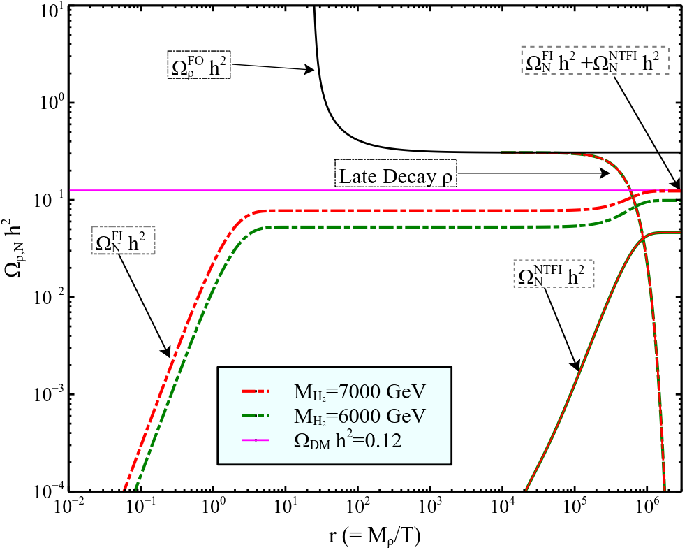
The dominance of non-thermal freeze-in production of DM is illustrated in Fig. 13 (left) for a benchmark point where GeV, GeV, GeV and . In evaluating the DM relic density, we assume that the initial abundance of was zero. At high temperature DM is produced through processes , and via thermal freeze-in. The decay is the dominant one. The NLOP, , first freezes-out and later undergoes out-of equilibrium decay (green-dashed line) thus increasing significantly the relic density of . The total production of taking into account both the thermal and non-thermal freeze-in is represented by the dot-dashed black line, and shows comparable contributions from both processes. When is much lighter than 2.4 TeV, its abundance is much suppressed and as expected the late decay contribution to is subdominant, this is illustrated in Fig. 13(right) where .
Note that the non-thermal freeze-in contribution depends on the mass ratio and the abundance of particle, i.e. at the time of decoupling. The mass of the heavy Higgs , of the charged Higgs and of the mixing angle have a negligible effect in determining , since the dominant annihilation channel of pairs is . The non-thermal freeze-in contribution does not depend on the Yukawa . Contrary to that, the thermal freeze-in contribution has a strong dependency on , and .
In Fig. 14, the variation of and abundances on these four model parameters is displayed. In the upper two panels, we show and for different choices of and , respectively. As discussed above, with an increase in , increases, thereby leading to a rise in the non-thermal freeze-in contribution until the factor provides significant suppression factor. This can be seen in the figure presented in the LP. The thermal freeze-in production on the other hand decreases with the increase in due to phase space suppression in the decay processes . For small value of , a linear increase of the DM abundance occurs due to thermal freeze-in production from , and decay. Altogether, we show the total DM relic density taking into account both the thermal and non-thermal freeze-in contributions. In the RP we show that both and increase with , this occurs as both these contributions are proportional to . In summary, the abundance and have different behaviour with respect to variations of and .
In the lower panel, we show the effect of different choices of and on DM and abundance. The thermal freeze-in contribution is proportional to the dark sector Yukawa coupling, and hence increases with an increase of . This can be seen from the LP. On the other hand, the non-thermal contribution is independent of the . In the RP, we show the effect of different choices BSM Higgs mass on DM and abundance. The abundance is independent of the BSM Higgs mass, as the dominant channel for is . instead increases with the increase in since its thermal contribution is inversely proportional to .
Among the different processes, the thermal production rate of DM is smaller for the process compared to process and due to additional mixing angle between the and .


5.2.3 Scan on parameter space
Three important parameters in determining the DM abundance are , and . We therefore vary these parameters in the following range while keeping GeV,
| (54) |
In the LP of Fig. 15, we show the points that reproduce the relic density in the plane of DM mass and the ratio of non-thermal freeze-in to the observed DM relic density. We observe that for fixed mass of DM, the ratio of non-thermal freeze-in to the observed relic density of DM increases as increases. As discussed above, the abundance of increases with and therefore leads to a large non-thermal freeze-in contribution to the DM relic density. The RP of Fig. 15 shows the scatter plot in the plane. Clearly, as the ratio of non-thermal freeze-in contribution to the observed relic density of DM increases, a smaller value of and a larger value of DM mass is required. The smaller value of the Yukawa coupling naturally leads to a suppressed thermal freeze-in contribution, which is essential to satisfy the DM relic density constraint. Contrary to that, a large Yukawa coupling is required to obtain a large thermal component of , thereby leading to a decrease in the ratio . The intersection point around GeV corresponds to equal contribution of and .


Impact of BBN constraints
The NLOP decays only via mode, producing significantly large non-thermal contribution to the DM relic density. The late decay of is therefore subject to cosmological constraints such as constraints arising from BBN discussed in section 4.4 or constraints on the amount of energy injected after sec that lead to spectral distortions of the CMB. The lifetime of has the following form
| (55) |

We consider two different constraints from a) CMB measurement and b) BBN constraints on light elements, namely the primordial mass fraction of , , as well as the ratio of abundances of and . These exclusions are taken from reference Kawasaki:2017bqm. In Fig. 16, we show the constraint in terms of lifetime and . The color code correspond to variations of Yukawa (for the LP) and of the Higgs mixing angle (for the RP). The points excluded by BBN correspond to small values of and/or , as with smaller and /or Higgs mixing angle, the lifetime of NLOP increases significantly.
In the LP of Fig. 17, we show contour plots for in the plane, as well as the regions which satisfy (green) and (grey), respectively. and are evaluated from Eq. 46 and Eq. 49 respectively where in the latter the partial decay width of is given by,
| (56) |
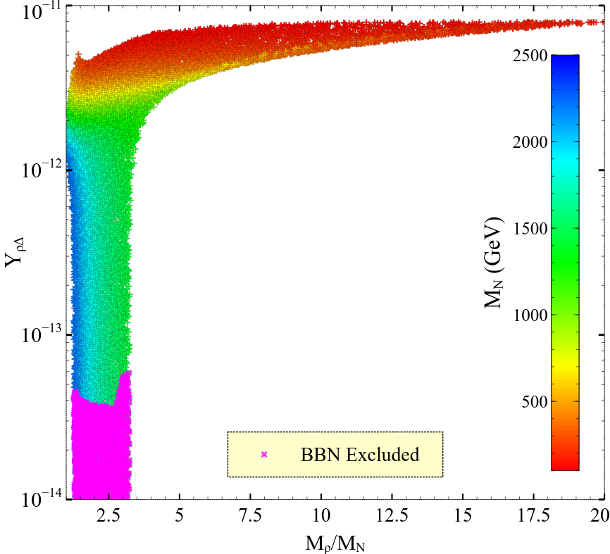
In the RP of Fig. 17, we show the allowed points after the relic density constraint in the plane for different masses of N. We can see that increases, as increases and it increases due to decrease in . This occurs due to the increase in thermal freeze-in contribution to the total relic density as increases. For a small value of , the non thermal freeze-in contributes significantly to the total relic density, thus negligible contribution from thermal freeze-in mechanism is required. Therefore, small value of is required when compared to the region with a large ratio of . This in turn leads to an increase in the lifetime of and gets severely constrained from BBN. The magenta points which corresponds to are disallowed by BBN.
5.3 DM production in Scenario III: a lighter scalar sector
In the previous sections, we have primarily focussed on DM production from the decay of BSM particles. Considering the chosen values for the DM mass, the BSM Higgs masses need to be at least a few TeV’s for decay processes to be kinematically allowed. One major drawback of having a heavy BSM Higgs is that they are difficult to be observed at the LHC. To include the possibility of lighter BSM Higgs masses, in this section we deviate from the assumption of decay dominance in DM production and also consider DM production from annihilation of SM/BSM particles. First we illustrate the impact of a lighter on the DM relic density including only decay processes. For this we consider a scenario where is the DM and is produced from the processes and , while is kinematically forbidden. We choose and different values of such that . In Fig.18, we show both the evolution of from freeze-out and its out-of equilibrium decays and of from thermal as well as non-thermal freeze-in mechanism. At low temperatures, the number density of is decreased by two processes, and contrary to the previous scenario where only the latter process was kinematically open. The corresponding production of from these decays, as computed from Eq.49 shows no dependence on . The thermal freeze-in contribution on the other hand increases with a decrease in the mass of . This occurs due to a decrease in the phase space suppression factor for the dominant process .


Although decays will typically contribute to DM formation, we found that for a lighter BSM Higgs the annihilation contribution can be as large as and that the DM relic density can be satisfied even for a few hundred GeVs BSM neutral Higgs and charged Higgs . To take into account the annihilation contribution, we implement the model in Feynrules Alloul:2013bka and generated the CalcHEP files Belyaev:2012qa that are fed to micrOMEGAs Belanger:2018ccd; Belanger:2022qxt. In studying the annihilation contribution, we consider two scenarios, a) is DM and and b) is DM and . For both of these scenarios, we consider the parameter space where the DM relic density varies in the following range,
| (57) |
In choosing this range we require the DM in this model to constitute at least 40% of the total DM content.
5.3.1 Fusion dominated scenario: and
In this regime, the triplet is a WIMP DM which is weakly coupled with the bath particles. As we have pointed out before, the relic density constraint for the freeze-out production of is satisfied only for TeV. For lighter , the thermal contribution to relic density is sub-dominant, while other production mechanisms can give large contributions.
We impose the DM relic density constraint in Eq. 57 and vary the model parameters in the following range,
| (58) |
where . Note that, since is a thermal DM, it is subject to constraints from direct and indirect detection experiments, which we discuss in Section. 4.2. Moreover, the lower value chosen for is in agreement with the disappearing track search limit from the LHC ATLAS:2022rme. Additionally, the chosen and range are also in agreement with the LHC constraints which we discuss in Section. 3. Below, we discuss the impact of our chosen range for the model parameters on DM observables.
The processes contributing to annihilation are shown in Fig. 19 and include and production processes such as , production as well as annihilation channels of the type , where (i = 1, 2). For the masses we consider, is produced off-shell and hence annihilation processes mediated by are suppressed. Annihilation processes mediated by are further suppressed by the small mixing angle. Moreover the decay mode, is not kinematically allowed. Thus, the major annihilation contribution arises from processes involving in the final state where the mediator is produced on-shell. The production of can be considered as fusion process , and then the produced undergoes two body decay. The corresponding Feynman diagram is the last diagram of Fig. 19.
The on-shell production of through production mode can be approximately expressed as Hall:2009bx,
where . Once is produced on-shell, it will eventually decay to DM contributing to its relic density, . For a very tiny , the decay of can however alter the BBN prediction.


The masses of the BSM Higgs, of and DM as well as the Yukawa coupling are the most important model parameters to determine the relic density. In Fig. 20, we show scatter plots in the and planes after demanding the DM relic density to be within the range mentioned in Eq. 57. The color bar in the LP and RP are for the mass difference and the BSM Higgs mass , respectively. On the LP we can see that for mass below 500 GeV, there are mostly green, red, yellow and black points which correspond to GeV. Since for this regime, there is no phase space suppression for the production of , hence, is produced on-shell and decay abundantly to DM. Therefore, there is no noticeable variation in the required coupling. Once we go beyond GeV, there are points that correspond to any mass splitting. The points with the larger mass splitting (red, yellow and green points) are confined to values for the same reason as above. However for the smaller mass splitting (blue and cyan points), higher values of are required, as in this region production of on-shell faces kinematic suppression. Therefore, to obtain the DM relic density for GeV, higher values of are required to enhance the production of . In the entire region, the primary decay mode is since the other allowed decay mode is suppressed due to small neutral Higgs mixing angle. In the RP, we show the allowed points in the plane where the color bar represents variation in . For GeV, the production of can encounter phase-space suppression hence requiring much higher values for . For GeV, phase space factor do not have any effect. The variation in Yukawa is solely guided by the chosen range of DM relic density. This is evident, that for both the LP and RP, the increase in occurs for similar values of between GeV, as for the chosen range of and , only in this range production of encounters phase-space suppression.


In the LP of Fig. 21, we show a scatter plot in the plane where the color points represent the variation in the Yukawa coupling . There is a sharp correlation between and as the DM relic density follows the relation . At GeV, a higher value of is required to satisfy the relic density, as is evident from the few green and yellow points. This occurs due to phase space suppression in the production of . For higher values of GeV, the maximum value of DM mass reaches upto 1350 GeV. For a heavier , the relic density from freeze-out contribution also becomes large, and hence after taking into account the late decay contribution from , the points which lie in the GeV range produce overabundant and hence are disallowed. Similarly the region corresponding to a high ratio is disallowed, since it leads to underabundant DM. On the other hand, the white region towards the left is where production encounters phase-space suppression and hence DM relic density is very low. In the RP, we show scatter plot in the plane and the color variation represents different values of . The points which satisfy correspond to the region where is kinematically not allowed. hence, in this region decay is dominant. Moreover in this region there is no phase-space suppression in the production of and a moderate value of is required when to maintain the DM relic density in the desired range. On the other hand, for the region , production is kinematically suppressed, which leads to a sudden rise in the required in order to obtain the DM relic density. For , the mass of is very large. In this region, decay is open and in addition, production of is also not limited by kinematics. Therefore, a moderate Yukawa is required.
5.3.2 Substantial Annhilation Contribution: and
In this regime, is a FIMP DM. This scenario is challenging to probe via direct and indirect DM detection experiments. However, as we will see, the decay of to visible particles along with DM can be probed at colliders. To obtain the DM relic density in the aforementioned range, Eq. 57, we have varied the model parameters as follows,
| (60) |
For most of the above mentioned parameters, the chosen range is similar to the previous scenario, except for , which in this case can also be in the sub-GeV range. As we will see, this has implication for the detection of this scenario at future experiments that search for long-lived particles (LLPs), such as MATHUSLA Curtin:2018mvb.


Note that, similar to the previous scenario, decay is kinematically forbidden, although standard freeze-in contribution and late decay contribution from can be large in part of the parameter space. The other significant contribution arises from the annihilation channels mediated via , where etc., see Fig. 19. Contrary to the previous scenario, these contributions can be large due to the choice of a lower DM mass. In the LP of Fig. 22, we show scatter plot in the plane where the color bar represents variation in the DM relic density. In this scenario, DM is primarily produced from the decay of , so the DM relic density can be expressed as, . To obtain the DM relic density in a specific range, and must follow . This dependency is clearly visible in the figure. For a fixed value of increase in leads to larger DM relic density, which is depicted by the red and black points. In the RP, we show the scatter plot in the plane. The different colors points represent the different contributions from the decay mode. The region below the dark magenta line corresponds to where mostly (A, B are the other bath particles) mediated via dominates. The region below the red line is ruled out from the 13 TeV disappearing track searches of the LHC with 136 data ATLAS:2022rme. For a fixed value of when increases the decay contribution dominates because of less phase space suppression for decay.


Although a FIMP DM is challenging to detect at DM direct and indirect detection experiment, and the NLOP in such scenario leaves no signature at the detector unless it is charged, detectors such as MATHUSLA can probe the long lived NLOP. In Fig. 23, we show the detection prospects for our model parameter space at the future MATHUSLA detector with a volume []. We display the production cross section of the LLP, , at the HL-LHC as function of the lifetime in the lab-frame where is the average boost factor Curtin:2018mvb and is the decay length of the long lived particle . The color bar represents the variation in () LP (RP). The region above the green line (which corresponds to GeV) is ruled out by the LHC 36.1 data from disappearing track searches ATLAS:2017oal and the region above the magenta dashed line (which corresponds to GeV) is ruled out by an updated search with a higher luminosity 136 data ATLAS:2022rme. The red solid line represents the projected sensitivity of MATHUSLA taken from Curtin:2018mvb. While the region with a cross-section of production above 12 fb is already ruled out by current LHC search, part of the remaining parameter space can be probed by MATHUSLA. In particular the region with a very light DM, (represented by white, blue and green points) as can be seen in LP of Fig. 23 falls within the sensitivity reach of MATHUSLA. Note that, large decay lengths correspond to the higher values of DM mass and to the small values of , as can be seen from RP of Fig. 23. As we have mentioned before the decay width of is proportional to and hence the decay length is inversely proportional to it. Moreover since , therefore and are anti-correlated. The main important message from Fig. 23 is that the MATHUSLA detector can be sensitive to DM mass in the MeV range while for heavier DM, the NLOP will decay outside the detector. Finally we have checked for both mass ranges i.e. and that our allowed parameter spaces are safe from the Lyman- constraints, in particular following Ref. Cembranos:2005us, we obtain a free streaming length less than Mpc.
6 Collider Prospects of triplet fermions and BSM Higgs
Before concluding, we present a brief discussion on fermion triplet () and BSM Higgs signature with the ATLAS and CMS detectors at the LHC.
In our model, the dark sector comprises of SM singlet and which is a part of electroweak multiplet. The mass of and of are degenrate at tree level to preserve the gauge invariance. However, the degeneracy is broken due to quantum correction from electroweak gauge boson and tends to make slightly heavier than . The mass splitting is proportional to which is numerically in order of MeV value. The increases as mass of increases and after which it becomes approximately constant for large mass of . Contrary to fermion triplet, the charged and neutral component of scalar triplet can have mass splitting at tree level due to extra renormalizable interaction with SM Higgs field. However, the mass splitting can’t be too large at tree level due to perturbative constraint (see Fig.1).
Since and form a compressed mass spectrum, can decay to along with charged lepton and neutrino when is less than the pion mass. For , decays to and and the branching fraction is approximately for this decay modeCirelli:2005uq. For our considered mass range of , the above mentioned decay primarly occurs. The decay width of has the following form Cirelli:2005uq,
| (61) |
The mass splitting between and ensures to be the DM component and makes to be a long lived particle. The decay product of ,i.e pions, are very soft and is stopped by the magnetic field of the detector. Thus, the pions leaves short track in the detector after which it disappears and hence can be considered as a MET. This disappearing track signature can be used to probe the DM multiplet () having compressed mass spectrum.
6.1 Disappearing track searches
There are dedicated LHC analyses of the disappearing track signature for the super symmetric particles such as charginos which are applicable to our model. The production as well as decay process of is similar to charginos. The ATLAS and CMS collaborations set bounds on the lifetime of charginos as a function of its mass. The maximum excluded mass of from the ATLAS disappearing track search with data is approximately around GeV ATLAS:2022rme. For our model, this puts a bound on the charged fermions() which is GeV (see Fig 2). The HL-LHC with of data will also be able to probe upto 870 GeV Dainese:2019rgk.


6.2 Scalar Triplet
The BSM Higgs plays an important role in the production of DM for both the scenarios where and are the DM candidates. Therefore, it becomes crucial to determine whether our choice of paramter spaces are allowed by LHC searches.
The primary production process for the neutral BSM Higgs in our scenarios at LHC is through Drell Yan production. The gluon-gluon fusion (ggF) and vector boson fusion (VBF) production mode for is suppressed compared to Drell Yan Production due to the suppression in the coupling of to heavy quarks and vector bosons (). Additionally, we also have pair production of the neutral BSM Higgs at LHC via off-shell SM Higgs. This production rate of depends on . In our analysis, we have assumed which ensures that for GeV and also guarantees production of via off-shell SM Higgs is suppressed. As a result, the primary production of BSM Higgs is via neutral or charged current Drell Yan production. In the LP of Fig. 24, we show the cross-sections for and for TeV LHC and TeV FCC-hh Golling:2016gvc colliders whereas in the RP we show the
production cross-section for c.o.m energy 1 TeV at ILC Baer:2013cma and 3 TeV
at CLIC CLICDetector:2013tfe.
- •
Production Process
- –
Drell-Yan pair production:- ,
- –
gg Fusion:- ,
- –
VB Fusion:-
- –
The different LHC contraints applicable for the BSM Higgs and its mixing are as follows,
- •
The signal strength of the SM Higgs is given by,
(62) where represents decay mode of the SM Higgs. The branching ratio of is almost identical to SM Higgs, 55 5 As the decay mode of is kinematically forbidden in our analysis.. The primary production mode of SM Higgs is through ggF and VBF. The prodution cross-section of can be written as . Therefore, the above signal strength can be approximated as,
(63) Figure 25: Branching fractions for and for different masses of . .
The global signal strength of is as measured by =13 TeV LHC ATLAS:2020qdt. This measurement puts an upper bound on the BSM-SM Higgs mixing angle and demands that should be smaller than 0.36. In our analysis, we have considered and our choosen parameters are in agreement with LHC constraints.
- •
The LHC searches for resonance BSM Higgs production through ggF and VBF and its decay to SM states. The main decay channels of BSM Higgs are and . The branching fraction for both and is shown in Fig.25. The ATLAS and CMS searches puts a limit on production cross-section of produced through ggF and VBF times branching fraction of . We have checked into following searches, ATLAS:2020tlo, ATLAS:2020fry and ATLAS:2019qdc and found that searches doesn’t constraint our parmater space at all.
- •
Higgs Diphoton rate:- The introduction of the real triplet scalar will lead to a correction to the SM Higgs diphoton rate via the addition of a newly charged scalar in the loop. For the light charged scalar, the SM Higgs diphoton rate is enhanced because of constructive interference between Higgs triplet and SM contribution. The enhancement in the diphoton rate will be proportional to coupling strength of the scalar potential. The SM Higgs partial width to diphoton is given by Wang:2013jba,
(64) In our scenario, the partial width of to diphoton is given by,
(65) where , are the electric charges of fermion and scalar. The vertex takes the form,
(66) From the expression of , it is clear that considering would only have a mild impact on and hence on .
The loop functions are given by,

Figure 26: Higgs diphoton Rate for different masses of assuming . The signal strength of SM Higgs to diphoton process is given by,
(67) Recent measurements by the ATLAS ATLAS:2018hxb and CMS CMS:2021kom are,
(68) For our analysis, we have assumed which ensures that the quartic coupling is positive and independent of the mass of . Due to this, is suppressed as the destructive interference occurs between the SM and Higgs triplet contribution. In Fig.26, we have shown that which increases with the increase in mass of .
In the LP and RP of Fig. 25 we have shown the branchings of and to different SM final states. In generating the plots, we have assumed that . As can be seen from the LP, in the mass range , the dominant decay mode is while in the mass range , the dominant mode is . Therefore, for the lower mass range the signature for production at either or colliders would be either or . On the other hand for the mass range , the final states are either . In RP we show that for the dominant decay mode is , for the whole mass range. Therefore, one can search for in the following final states , , and . Note that, as seen in Fig. 24, the production cross-section for at collider falls sharply at high masses for TeV and is lower than in collisions. Thus it could be advantageous to study this process at a high energy collider than the TeV pp collider. Moreover, we need a full fledged collider study in order to compare the signal superiority between the proposed for TeV and 100 TeV FCC-hh colliders. The detailed study of the collider prospects for different final states including the associated backgrounds is left for future work.
7 Conclusion
In this work, we have extended the SM by adding one singlet fermion, three triplet fermions and one triplet scalar with hypercharge zero for all the additional particles. The new particles can solve two well-accepted SM problems namely a dark matter candidate and the origin of the neutrino mass. When the triplet scalar acquires a vev, it generates a mixing between the neutral component of the triplet fermion and the singlet fermion which are odd under symmetry. The lightest of these particles becomes a suitable dark matter candidate while the NLOP eventually decays to the DM candidate. The NLOP is typically long-lived. The remaining two triplet fermions which are even under the symmetry take part in the generation of neutrino masses and the bounds on the neutrino oscillation parameters can be very easily satisfied. In exploring the viable parameter space of the model we impose the strict range on the DM relic density obtained from PLANCK observations of the CMB. We have also taken into account bounds on the mass of the fermion triplet from the disappearing track search at the ATLAS and CMS detectors as well as current bounds from direct and indirect searches of DM which apply only to the WIMP DM. Morever we found that the neutral and charged components of the scalar triplet are nearly degenerate when imposing a perturbative bound on the quartic couplings.
To investigate the possible DM formation mechanisms, we have considered two mass regimes corresponding to the lightest stable DM particle being the triplet dominated fermion or the singlet dominated fermion . In both regimes, the NLOP can decay to the DM candidate and a scalar particle thus injecting extra hadronic energy in the Universe. Depending on the coupling strength, the late decay might happen during the BBN and thus alter the light elements (H, D, He, Li) abundance. We have imposed constraints from BBN and found the model to be viable in large areas of parameter space.
For the mass range , DM can be produced by thermal freeze-out and by the late decay of the NLOP . The presence of the late decay production mode means that the correct value for the DM relic density for the triplet can be reached even for masses below TeV while the freeze-out mechanism by itself requires a mass above 2.4 TeV. The NLOP can be produced by the freeze-in mechanism from the decay of the BSM Higgs , the annihilation of bath particles and fusion processes. The dominant production mode depends on the masses of the NLOP and of other particles involved in its production. Since the NLOP never reaches thermal equilibrium, in order to properly take into account its decay contribution to DM, we have determined the NLOP distribution function and used it in the subsequent DM production.
In the mass regime , DM never reaches thermal equilibrium with the cosmic soup, so it is produced by the freeze-in mechanism through the decay, annihilation and fusion of the bath particles. Depending on the mass of DM and other new particles either/all of them actively contribute to DM production. Moreover, DM is also produced from the late decay of the NLOP by the superWIMP mechanism. In this case we showed that DM could be detected indirectly at the MATHUSLA detector from the late decay of NLOP or by reconstructing the displaced vertex and missing energy searches at the ATLAS and CMS detectors.
In conclusion in both regimes there remains a possibility for detection of DM even if it is produced mainly by the freeze-in mechanism. Moreover we have briefly discussed the possibility of triplet fermion and Higgs detection prospects at the LHC, a more extensive study of collider prospects is left for future work.
Acknowledgements
This work was funded in part by the Indo-French Centre for the Promotion of Advanced Research (Project title: Beyond Standard Model Physics with Neutrino and Dark Matter at Energy, Intensity and Cosmic Frontiers, Grant no: 6304-2). This work used the Scientific Compute Cluster at GWDG, the joint data center of Max Planck Society for the Advancement of Science (MPG) and University of Göttingen. AR acknowledges SAMKHYA: High-Performance Computing Facility provided by the Institute of Physics (IoP), Bhubaneswar.
Appendix A Appendix
A.1 Analytical expressions for thermal average cross-section
The analytical expression for DM annihilation and co-annihilation channels are as follows Ma:2008cu,
| (69) |
Thermal average of the above cross sections takes the following form,
where , and () .
A.2 Collision function
The collision function for the production of the next to lighest neutral fermion from the decay of the BSM Higgs has the following form,
where and is the initial value of . The amplitude for the process can be expressed as,
| (72) |
where , and . The parameters and can be expressed as66 6 is the momentum used in the phase space integration,
| (73) |
where is given by
A.3 Decay Widths
The decay width for the process can be expressed as,
References
- (1) Planck collaboration, P. Ade et al., Planck 2015 results. XIII. Cosmological parameters, Astron. Astrophys. 594 (2016) A13, [1502.01589].
- (2) L. J. Hall, K. Jedamzik, J. March-Russell and S. M. West, Freeze-In Production of FIMP Dark Matter, JHEP 03 (2010) 080, [0911.1120].
- (3) J. L. Feng, A. Rajaraman and F. Takayama, Superweakly interacting massive particles, Phys. Rev. Lett. 91 (2003) 011302, [hep-ph/0302215].
- (4) R. Foot, H. Lew, X. G. He and G. C. Joshi, Seesaw Neutrino Masses Induced by a Triplet of Leptons, Z. Phys. C 44 (1989) 441.
- (5) S. Choubey, S. Khan, M. Mitra and S. Mondal, Singlet-Triplet Fermionic Dark Matter and LHC Phenomenology, Eur. Phys. J. C 78 (2018) 302, [1711.08888].
- (6) P. Chardonnet, P. Salati and P. Fayet, Heavy triplet neutrinos as a new dark matter option, Nucl. Phys. B 394 (1993) 35–72.
- (7) M. Cirelli, N. Fornengo and A. Strumia, Minimal dark matter, Nucl. Phys. B 753 (2006) 178–194, [hep-ph/0512090].
- (8) Particle Data Group collaboration, P. A. Zyla et al., Review of Particle Physics, PTEP 2020 (2020) 083C01.
- (9) J. Erler and P. Langacker, Electroweak model and constraints on new physics, hep-ph/0407097.
- (10) J. Erler and P. Langacker, Electroweak Physics, Acta Phys. Polon. B 39 (2008) 2595–2610, [0807.3023].
- (11) CDF collaboration, T. Aaltonen et al., High-precision measurement of the W boson mass with the CDF II detector, Science 376 (2022) 170–176.
- (12) M.-C. Chen, S. Dawson and C. B. Jackson, Higgs Triplets, Decoupling, and Precision Measurements, Phys. Rev. D 78 (2008) 093001, [0809.4185].
- (13) ATLAS collaboration, G. Aad et al., Search for type-III seesaw heavy leptons in leptonic final states in collisions at TeV with the ATLAS detector, 2202.02039.
- (14) ATLAS collaboration, A combination of measurements of Higgs boson production and decay using up to fb-1 of proton–proton collision data at 13 TeV collected with the ATLAS experiment, .
- (15) ATLAS collaboration, M. Aaboud et al., Measurements of Higgs boson properties in the diphoton decay channel with 36 fb-1 of collision data at TeV with the ATLAS detector, Phys. Rev. D 98 (2018) 052005, [1802.04146].
- (16) ATLAS collaboration, G. Aad et al., Search for heavy resonances decaying into a pair of Z bosons in the and final states using 139 of proton–proton collisions at TeV with the ATLAS detector, Eur. Phys. J. C 81 (2021) 332, [2009.14791].
- (17) ATLAS collaboration, G. Aad et al., Search for heavy diboson resonances in semileptonic final states in pp collisions at TeV with the ATLAS detector, Eur. Phys. J. C 80 (2020) 1165, [2004.14636].
- (18) ATLAS collaboration, M. Aaboud et al., Search for long-lived charginos based on a disappearing-track signature in pp collisions at TeV with the ATLAS detector, JHEP 06 (2018) 022, [1712.02118].
- (19) ATLAS collaboration, G. Aad et al., Search for long-lived charginos based on a disappearing-track signature using 136 fb-1 of collisions at = 13 TeV with the ATLAS detector, 2201.02472.
- (20) CMS collaboration, A. M. Sirunyan et al., Search for disappearing tracks as a signature of new long-lived particles in proton-proton collisions at 13 TeV, JHEP 08 (2018) 016, [1804.07321].
- (21) A. Dainese, M. Mangano, A. B. Meyer, A. Nisati, G. Salam and M. A. Vesterinen, eds., Report on the Physics at the HL-LHC,and Perspectives for the HE-LHC, vol. 7/2019 of CERN Yellow Reports: Monographs. CERN, Geneva, Switzerland, 2019, 10.23731/CYRM-2019-007.
- (22) XENON collaboration, E. Aprile et al., Dark Matter Search Results from a One Ton-Year Exposure of XENON1T, Phys. Rev. Lett. 121 (2018) 111302, [1805.12562].
- (23) PandaX collaboration, J. Liu, The first results of PandaX-4T, Int. J. Mod. Phys. D 31 (2022) 2230007.
- (24) LUX-ZEPLIN collaboration, J. Aalbers et al., First Dark Matter Search Results from the LUX-ZEPLIN (LZ) Experiment, 2207.03764.
- (25) MAGIC, Fermi-LAT collaboration, M. L. Ahnen et al., Limits to Dark Matter Annihilation Cross-Section from a Combined Analysis of MAGIC and Fermi-LAT Observations of Dwarf Satellite Galaxies, JCAP 02 (2016) 039, [1601.06590].
- (26) A. Reinert and M. W. Winkler, A Precision Search for WIMPs with Charged Cosmic Rays, JCAP 01 (2018) 055, [1712.00002].
- (27) T. Hambye, M. H. G. Tytgat, J. Vandecasteele and L. Vanderheyden, Dark matter direct detection is testing freeze-in, Phys. Rev. D 98 (2018) 075017, [1807.05022].
- (28) G. Bélanger, C. Delaunay, A. Pukhov and B. Zaldivar, Dark matter abundance from the sequential freeze-in mechanism, Phys. Rev. D 102 (2020) 035017, [2005.06294].
- (29) J. Hisano, K. Ishiwata, N. Nagata and T. Takesako, Direct Detection of Electroweak-Interacting Dark Matter, JHEP 07 (2011) 005, [1104.0228].
- (30) J. Hisano, S. Matsumoto and M. M. Nojiri, Explosive dark matter annihilation, Phys. Rev. Lett. 92 (2004) 031303, [hep-ph/0307216].
- (31) J. Hisano, S. Matsumoto, M. M. Nojiri and O. Saito, Non-perturbative effect on dark matter annihilation and gamma ray signature from galactic center, Phys. Rev. D 71 (2005) 063528, [hep-ph/0412403].
- (32) M. Kawasaki, K. Kohri, T. Moroi and Y. Takaesu, Revisiting Big-Bang Nucleosynthesis Constraints on Long-Lived Decaying Particles, Phys. Rev. D 97 (2018) 023502, [1709.01211].
- (33) E. Ma and D. Suematsu, Fermion Triplet Dark Matter and Radiative Neutrino Mass, Mod. Phys. Lett. A 24 (2009) 583–589, [0809.0942].
- (34) CMS collaboration, A. M. Sirunyan et al., Search for disappearing tracks in proton-proton collisions at 13 TeV, Phys. Lett. B 806 (2020) 135502, [2004.05153].
- (35) J. König, A. Merle and M. Totzauer, keV Sterile Neutrino Dark Matter from Singlet Scalar Decays: The Most General Case, JCAP 11 (2016) 038, [1609.01289].
- (36) E. W. Kolb and M. S. Turner, The Early Universe, vol. 69. 1990, 10.1201/9780429492860.
- (37) P. Gondolo and G. Gelmini, Cosmic abundances of stable particles: Improved analysis, Nucl. Phys. B 360 (1991) 145–179.
- (38) J. Edsjo and P. Gondolo, Neutralino relic density including coannihilations, Phys. Rev. D 56 (1997) 1879–1894, [hep-ph/9704361].
- (39) K. Jedamzik, Big bang nucleosynthesis constraints on hadronically and electromagnetically decaying relic neutral particles, Phys. Rev. D 74 (2006) 103509, [hep-ph/0604251].
- (40) A. Alloul, N. D. Christensen, C. Degrande, C. Duhr and B. Fuks, FeynRules 2.0 - A complete toolbox for tree-level phenomenology, Comput. Phys. Commun. 185 (2014) 2250–2300, [1310.1921].
- (41) A. Belyaev, N. D. Christensen and A. Pukhov, CalcHEP 3.4 for collider physics within and beyond the Standard Model, Comput. Phys. Commun. 184 (2013) 1729–1769, [1207.6082].
- (42) G. Bélanger, F. Boudjema, A. Goudelis, A. Pukhov and B. Zaldivar, micrOMEGAs5.0 : Freeze-in, Comput. Phys. Commun. 231 (2018) 173–186, [1801.03509].
- (43) G. Belanger, A. Mjallal and A. Pukhov, WIMP and FIMP dark matter in the inert doublet plus singlet model, 2205.04101.
- (44) D. Curtin et al., Long-Lived Particles at the Energy Frontier: The MATHUSLA Physics Case, Rept. Prog. Phys. 82 (2019) 116201, [1806.07396].
- (45) J. A. R. Cembranos, J. L. Feng, A. Rajaraman and F. Takayama, SuperWIMP solutions to small scale structure problems, Phys. Rev. Lett. 95 (2005) 181301, [hep-ph/0507150].
- (46) I. Hinchliffe, A. Kotwal, M. L. Mangano, C. Quigg and L.-T. Wang, Luminosity goals for a 100-TeV pp collider, Int. J. Mod. Phys. A 30 (2015) 1544002, [1504.06108].
- (47) A. Robson and P. Roloff, Updated CLIC luminosity staging baseline and Higgs coupling prospects, 1812.01644.
- (48) T. Golling et al., Physics at a 100 TeV pp collider: beyond the Standard Model phenomena, 1606.00947.
- (49) The International Linear Collider Technical Design Report - Volume 2: Physics, 1306.6352.
- (50) CLIC Detector, Physics Study collaboration, H. Abramowicz et al., Physics at the CLIC e+e- Linear Collider – Input to the Snowmass process 2013, in Community Summer Study 2013: Snowmass on the Mississippi, 7, 2013. 1307.5288.
- (51) ATLAS collaboration, G. Aad et al., Combination of searches for Higgs boson pairs in collisions at 13 TeV with the ATLAS detector, Phys. Lett. B 800 (2020) 135103, [1906.02025].
- (52) L. Wang and X.-F. Han, LHC diphoton and Z+photon Higgs signals in the Higgs triplet model with Y = 0, JHEP 03 (2014) 010, [1303.4490].
- (53) CMS collaboration, A. M. Sirunyan et al., Measurements of Higgs boson production cross sections and couplings in the diphoton decay channel at = 13 TeV, JHEP 07 (2021) 027, [2103.06956].