跳到论文正文
W Papers独立论文阅读器 arXiv:2208.00730 论文正文 计算阅读时间 · 0%
引用这篇论文根据当前论文元数据生成,正式投稿前建议核对。


License: arXiv.org perpetual non-exclusive license
arXiv:2208.00730v3 [cond-mat.str-el] 06 Jan 2023

Field-theoretic functional renormalization group formalism for non-Fermi liquids and its application to the antiferromagnetic quantum critical metal in two dimensions

Francisco Borges1,2 Affiliation: 1Department of Physics & Astronomy, McMaster University, Hamilton ON L8S 4M1, Canada    Anton Borissov1,2 Affiliation: 1Department of Physics & Astronomy, McMaster University, Hamilton ON L8S 4M1, Canada    Ashutosh Singh1,3 Note: Current address: Department of Physics & Astronomy, Texas A&M University, College Station Texas 77843, United States Affiliation: 1Department of Physics & Astronomy, McMaster University, Hamilton ON L8S 4M1, Canada    Andrés Schlief1,2,4 Note: Current address: Deutsche Bank, Berlin, Germany Affiliation: 1Department of Physics & Astronomy, McMaster University, Hamilton ON L8S 4M1, Canada    Sung-Sik Lee1,2 Note: slee@mcmaster.ca Affiliation: 1Department of Physics & Astronomy, McMaster University, Hamilton ON L8S 4M1, Canada Affiliation: 2Perimeter Institute for Theoretical Physics, Waterloo ON N2L 2Y5, Canada Affiliation: 3 Department of Physics, National Tsing Hua University, Hsinchu 300013, Taiwan Affiliation: 4Max-Planck-Institut für Physik Komplexer Systeme, 01187, Dresden, Germany
August 11, 2026
Abstract

To capture the universal low-energy physics of metals within effective field theories, one has to generalize the usual notion of scale invariance and renormalizable field theory due to the presence of intrinsic scales (Fermi momenta). In this paper, we develop a field-theoretic functional renormalization group formalism for full low-energy effective field theories of non-Fermi liquids that include all gapless modes around the Fermi surface. The formalism is applied to the non-Fermi liquid that arises at the antiferromagnetic quantum critical point in two space dimensions. In the space of coupling functions, an interacting fixed point arises at a point with momentum-independent couplings and vanishing nesting angle. In theories deformed with non-zero nesting angles, coupling functions acquire universal momentum profiles controlled by the bare nesting angles at low energies before flowing to superconducting states in the low-energy limit. The superconducting instability is unavoidable because lukewarm electrons that are coherent enough to be susceptible to pairing end up being subject to a renormalized attractive interaction with its minimum strength set by the nesting angle irrespective of the bare four-fermion coupling. Despite the inevitable superconducting instability, theories with small bare nesting angles and bare four-fermion couplings that are repulsive or weakly attractive must pass through the region with slow RG flow due to the proximity to the non-Fermi liquid fixed point. The bottleneck region controls the scaling behaviours of the normal state and the quasi-universal pathway from the non-Fermi liquid to superconductivity. In the limit that the nesting angle is small, the non-Fermi liquid scaling dictates the physics over a large window of energy scale above the superconducting transition temperature.

Notation

  1. 1.

    scales

    • •

      Λ\Lambda : UV energy cutoff

    • •

      kFk_{F} : size of Fermi surface

    • •

      μ\mu : floating energy scale at which renormalization conditions are imposed

  2. 2.

    momentum

    • •

      k→=(kx,ky)\vec{k}=(k_{x},k_{y}) : two-dimensional momentum measured with respect to the hot spot in each patch

    • •

      𝐤=(k0,k→){\bf k}=(k_{0},\vec{k}) : three-momentum vector made of Matsubara frequency and two-dimensional momentum

    • •

      Q→A​F\vec{Q}_{AF} : the antiferromagnetic ordering vector

    • •

      kNk_{N} : the component of k→\vec{k} that is perpendicular to Q→A​F\vec{Q}_{AF}

    • •

      kk : abbreviation for kNk_{N} used when the associated hot spot index is obvious

    • •

      k⟂k_{\perp} : the component of k→\vec{k} that is parallel to Q→A​F\vec{Q}_{AF}

    • •

      K=k​eℓK=ke^{\ell} : rescaled momentum associated with the logarithmic length scale ℓ\ell

  3. 3.

    coupling functions

    • •

      VF,kV_{F,k} : the momentum dependent Fermi velocity parallel to the antiferromagnetic ordering vector

    • •

      vkv_{k} : the momentum dependent local nesting angle

    • •

      cc : the speed of the overdamped collective spin fluctuation

    • •

      wk≡vk/cw_{k}\equiv v_{k}/c (w≡v0/cw\equiv v_{0}/c)

    • •

      gk,pg_{k,p} : the momentum dependent fermion-boson coupling function

    • •

      λ(k1k2k4k3)(N1N2N4N3);(σ1σ2σ4σ3){\lambda}^{\begin{pmatrix}N_{1}&N_{2}\\ N_{4}&N_{3}\end{pmatrix};\begin{pmatrix}\sigma_{1}&\sigma_{2}\\ \sigma_{4}&\sigma_{3}\end{pmatrix}}_{\begin{pmatrix}k_{1}&k_{2}\\ k_{4}&k_{3}\end{pmatrix}} : the momentum dependent four-fermion coupling function

    • •

      uau_{a} (a=1,2a=1,2) : quartic boson couplings

I Introduction

One of the major goals in condensed matter physics is to understand universal relations that low-energy observables satisfy through effective theories. While the richness of condensed matter physics comes from the great variety of low-energy effective theories that can emergeWen 2004; Sachdev 2011; Fradkin 2013; Tsvelik 2003; Coleman 2015; Burgess 2020, the power of low-energy effective theories is derived from their insensitivity to microscopic detailsKadanoff 1966; Wilson 1971a; Wilson 1971b. In no small part, the remarkable progress in modern condensed matter physics is attributed to the balance between the diversity and the universality that our nature granted.

Crudely, different types of low-energy effective theories can be classified in terms of the number of low-energy modes. In the trivial insulator, there is no low-energy degree of freedom, and the theory is empty in the infrared limit. In topological states, there can be low-energy modes but their number scales sub-extensively with the volume of system due to the non-local nature of excitations. In states with gapless local excitations, the number of low-energy modes is extensive. Gapless states can be further divided into sub-classes in terms of the dimension of the manifold where gapless single particle excitations reside in momentum space. In systems with emergent Lorentz symmetry, zero-energy modes reside at discrete points in momentum space. In those theories, the universal low-energy physics is encoded in a discrete set of operators classified in terms of their scaling dimensions and chargesDi Francesco et al. 1997; Rattazzi et al. 2008. In metals, on the other hand, there are infinitely many gapless modes residing on extended Fermi surfaces, and one needs function’s worth of data to fully characterize the universal low-energy physics.

In Fermi liquidsLandau 1957; Shankar 1994; Polchinski 1992, the low-energy physics is specified by the topology and geometric shape of the Fermi surface, the Berry phase around the Fermi surfaceHaldane 2004, the angle-dependent effective mass and the forward scattering amplitude. The simplicity of the low-energy effective theory of Fermi liquids is due to the existence of well-defined quasiparticles11 1 Well-defined quasiparticles imply a large emergent symmetry groupHaldane 2005, but the converse is not necessarily true. It has been recently pointed out that a large emergent symmetry group can be a general feature of compressible states beyond the quasiparticle paradigmElse et al. 2021. . In non-Fermi liquids, however, the quasiparticle picture is not validStewart 2001; Schofield 1999, and extracting dynamical information out of effective field theories is significantly harderHolstein et al. 1973; Hertz 1976; Lee 1989; Reizer 1989; Lee and Nagaosa 1992; Millis 1993; Altshuler et al. 1994; Kim et al. 1994; Nayak and Wilczek 1994; Polchinski 1994; Abanov and Chubukov 2000; Abanov et al. 2003; Abanov and Chubukov 2004; Löhneysen et al. 2007; Senthil 2008; Lee 2009; Mross et al. 2010; Metlitski and Sachdev 2010a; Metlitski and Sachdev 2010b; Hartnoll et al. 2011; Abrahams and Wölfe 2012; Jiang et al. 2013; Fitzpatrick et al. 2013; Dalidovich and Lee 2013; Strack and Jakubczyk 2014; Sur and Lee 2014; Patel and Sachdev 2014; Sur and Lee 2015; Ridgway and Hooley 2015; Holder and Metzner 2015; Patel et al. 2015; Varma 2015; Eberlein 2015a; Schattner et al. 2016a; Sur and Lee 2016; Liu et al. 2018a; Xu et al. 2017; Liu et al. 2017; Chowdhury et al. 2018; Varma et al. 2018; Berg et al. 2018; Liu et al. 2018b22 2 For recent progress in non-Fermi liquid theories with random couplings, see Refs Sachdev and Ye 1993; Kitaev; Maldacena and Stanford 2016; Wu et al. 2018; Esterlis et al. 2021. . Among the additional data that are needed for non-Fermi liquids are the singularity of the critical Fermi surface characterized by anomalous dimensions of fermions, dynamical critical exponents, and scaling properties of other critical modes that are present in the systemSenthil 2008. Since the momentum along the Fermi surface plays the role of a continuous flavour, critical exponents (such as the scaling dimension of fermions) can depend on the momentum along the Fermi surface.

One approach to non-Fermi liquids that has proven to be useful is the patch theory33 3 See Lee 2018 for a recent review.. The goal of a patch theory is to ‘divide and conquer’ the full theory by considering only a minimal set of patches of Fermi surface at a time. The patch description is valid if large-momentum scatterings that connect different parts of Fermi surface are negligible. When the interactions mediated by critical collective modes are sufficiently singular at low momenta, large-angle scatterings are dynamically suppressed. In two space dimensions, two fermions on the Fermi surface can stay close to the Fermi surface while exchanging a boson with a small momentum only when those fermions are in patches that are parallel or anti-parallelPolchinski 1994. In this case, regions of Fermi surface with different orientations are not strongly coupled, and the patch theory is a good description at least within a range of energy scales in which inter-patch scatterings can be ignored.

However, the patch theory has its limitations. In metals that support two-dimensional Fermi surface, the patch description is not valid at any energy scale as fermions in any two patches can be scattered along a common tangential direction while staying close to the Fermi surface. Even for one-dimensional Fermi surfaces44 4 This includes metals in two space dimensions and semi-metals with line nodes in three dimensions. , the patch theory breaks down if large-momentum scatterings are not suppressed. This may happen in marginal Fermi liquidsVarma et al. 1989 where the interaction mediated by a gapless collective mode is not singular enough to suppress large-angle scatterings of electrons along the Fermi surfaceYe et al. 2022. Inter-patch couplings become also important in the presence of strong superconducting fluctuationsAbanov and Chubukov 2020; Wu et al. 2020a; Wu et al. 2020b; Wu et al. 2021a; Wu et al. 2021b; Zhang et al. 2021; Wang et al. 2017a; Raghu et al. 2015; Mandal 2016 or impuritiesJang and Kim 2021 that scatter electrons around the Fermi surface. Furthermore, the patch theory is not ideal for describing momentum-dependent scaling properties of fermions because it includes only a fraction of Fermi surface. Although one can ‘patch’ multiple patch theories to capture global aspects of Fermi surfaceSon 1999; Metlitski et al. 2015, it is desirable to have one unified low-energy effective field theory description that includes all gapless degrees of freedom on the equal footing. It is also more convenient to include all low-energy modes within one theory to keep track of the anomalyElse et al. 2021; Darius Shi et al. 2022 because the anomaly is guaranteed to be preserved under the renormalization group flow only for the entire systemHooft 1980.

To capture the low-energy physics of the whole Fermi surface, the patch theory has to be extended to a theory that includes all gapless modes around the Fermi surface. Such theories are characterized by couplings that are functions of momentum along the Fermi surface. The universal low-energy data should be encoded in fixed points that arise in the space of coupling functions. Ultimately, one would like to identify the space of fixed points and extract the universal data associated with each fixed point. The natural theoretical framework for this is the functional renormalization group methodPolchinski 1984; Wetterich 1993 Morris 1994; Reuter 1998; Rosa et al. 2001; Höfling et al. 2002; Honerkamp 2008; Gies et al. 2010; Gies and Janssen 2010; Braun et al. 2011; Metzner et al. 2012; Platt et al. 2013a; Zanchi and Schulz 2000; Wang et al. 2009; Halboth and Metzner 2000; Scherer et al. 2012; Janssen and Gies 2012; Mesterházy et al. 2012; Lee et al. 2013; Eberlein and Metzner 2013; Platt et al. 2013b; Wang et al. 2014; Janssen and Herbut 2014; Maier et al. 2014; Eberlein 2014; Eberlein 2015b; Jakubczyk and Eberlein 2016; Maier and Strack 2016; Torres et al. 2018. The functional renormalization group flow describes how the momentum dependent vertex function evolves as a function of an energy scale. However, the exact renormalization group equation for the full vertex function is usually too difficult to solve for interacting theories. As a result, some forms of truncation, which are often uncontrolled, are employed to make the flow equation manageable. Fortunately, one does not need to know the full momentum-dependent vertex function to characterize the universal low-energy physics. Because gapless modes are residing on Fermi surface with a dimension lower than the space dimension, one should be able to throw away a great deal of non-universal information associated with modes away from the Fermi surface. For relativistic field theories, there exists a systematic way of achieving this : renormalizable field theory. Born out of the locality principle and the gradient expansion, a renormalizable field theory is the minimal theory that captures the low-energy physics shared by all theories within one universality class. They are simple enough that one can in principle study them with pen and paper, yet powerful enough to produce among the most accurate predictions in the physical sciencesGabrielse et al. 2006. Then, it is natural to combine the functional renormalization group formalism with the notion of renormalizable field theory to capture the universal low-energy physics of metals. The purpose of this work is to achieve this goal 55 5 For alternative approaches based on bosonization, see Refs. Castro Neto and Fradkin 1994; Houghton et al. 2000; Delacretaz et al. 2022. . In this paper, we develop a field-theoretic functional renormalization group formalism for general interacting theories of Fermi surface, and apply it to the non-Fermi liquid that arises at the antiferromagnetic quantum critical point in two space dimensions.

The antiferromagnetic quantum critical metal is potentially relevant to electron doped cupratesHelm et al. 2010, iron pnictidesHashimoto et al. 2012, and heavy fermion compoundsPark et al. 2006. The theory has been intensively studied both in field theoretical and numerical approachesAbanov and Chubukov 2000; Abanov et al. 2003; Abanov and Chubukov 2004; Hartnoll et al. 2011; Abrahams and Wölfe 2012; Lee et al. 2013; de Carvalho and Freire 2013; de Carvalho and Freire 2014; Patel et al. 2015; Patel and Sachdev 2014; Varma 2015; Maier and Strack 2016; Varma et al. 2018; Metlitski and Sachdev 2010b; Sur and Lee 2015; Sur and Lee 2016; Lee 2018; Berg et al. 2012; Li et al. 2016; Schattner et al. 2016b; Gerlach et al. 2017; Li et al. 2017; Wang et al. 2018. For the antiferromagnetic quantum critical metal in two dimensions, the minimal patch description includes the critical spin fluctuations and electrons residing near the hot spots. Here the hot spots refer to points on the Fermi surface connected by the antiferromagnetic wave vector and remain strongly coupled with spin fluctuations at low energies. Although the theory in two dimensions is strongly coupled at low energies, a recent study has revealed a strongly coupled fixed point where exact critical exponents can be obtainedSchlief et al. 2017. The fixed point is characterized by the anomalous dimension of the spin fluctuations 11, the dynamical critical exponent z=1z=1 and an emergent nesting of Fermi surface near the hot spots. Due to a slow flow of the nesting angle under the RG flow, at finite length scales one expects to see scaling behaviours controlled by transient exponents that depend on the nesting angleLunts et al. 2017. A recent quantum Monte Carlo studyLunts et al. 2022 that employs a sign problem-free lattice regularizationBerg et al. 2012; Gerlach et al. 2017; Berg et al. 2018; Schattner et al. 2016b shows scaling behaviours that are in qualitative agreement with the predictions.

However, the hot-spot theory is not complete because the antiferromagnetic quantum critical metal hosts both incoherent electrons near the hot spots and electrons with long lifetime away from the hot spots. The hot-spot theory is not capable of describing the momentum dependent universal properties of electrons on the Fermi surface and potentially important interplay between hot and cold electrons for superconductivityWang et al. 2017b. The patch theory does not include the four-fermion coupling either because it is irrelevant in the scaling that leaves the patch theory invariant. However, the four-fermion coupling should play an important role for superconductivity, which is another indication that the patch theory is incomplete. If the four-fermion coupling can give rise to infrared singularity, it is actually relevant for the low-energy physics. Superconducting fluctuations captured by the four-fermion coupling can be intrinsic features of non-Fermi liquid states. In this work, we include all gapless modes around the Fermi surface and the four-fermion coupling. For the full low-energy effective field theory, we answer the following questions:

  • •

    Q. How do quasiparticles in cold region gradually lose their coherence as one approaches the hot spots in the momentum space Abanov et al. 2003; Lee et al. 2013?

    A. Electrons at the hot spots are incoherent as they remain coupled with spin fluctuations at all energy scales. On the other hand, electrons away from the hot spots decouple from spin fluctuations below a crossover energy scale that increases as one moves away from the hot spots. This creates a critical fan for the electron spectral function in the momentum space (Fig. 27). At a fixed momentum along the Fermi surface, the single-electron decay rate exhibits a crossover from a non-Fermi liquid to the Fermi liquid behaviours as the momentum perpendicular to the Fermi surface (energy) is lowered. The crossover, in turn, determines the momentum-dependent quasiparticle weight of the electrons on the Fermi surface and the shape of the deformed Fermi surface. As one approaches the hot spots on the Fermi surface, the quasiparticle weight decays toward zero (Fig. 29) and the shape of the Fermi surface is deformed in such a way that the nesting is enhanced near the hot spots (Fig. 28).

  • •

    Q. How do spin fluctuations make electrons incoherent yet glue them into Cooper pairs? Is the pairing glue strong enough to overcome the pair breaking effect of the gapless collective modeAbanov and Chubukov 2020; Wu et al. 2020a; Wu et al. 2020b; Wu et al. 2021a; Wu et al. 2021b; Zhang et al. 2021; Wang et al. 2017a; Raghu et al. 2015; Mandal 2016?

    A. The gapless spin fluctuations provide the pairing glue, and at the same time they make electrons incoherent, which has the pair-breaking effect. Although the pair-breaking effect is significant near the hot spots, pairing instability prevails at sufficiently low energies. This is because (1) electrons away from the hot spots eventually become coherent at sufficiently low energies, (2) the high-energy spin fluctuations generate an attractive four-fermion interaction that coherent electrons become subject to at low energies, and (3) the minimum attractive four-fermion interaction is set by the bare nesting angle formed by the patches of Fermi surface connected by the antiferromagnetic ordering wave vector. The largely coherent electrons subject to the attractive interaction do not suffer from significant pair-breaking effect.

  • •

    Q. If pairing instabilities are present, do electrons near the hot spots that are subject to strong interactions but small in number drive superconductivity, or do abundant but cold electrons lead the instability?

    A. Electrons near the hot spots are too incoherent to drive superconducting instability by themselves despite the fact that they are subject to the strongest attractive interaction mediated by spin fluctuations. Cold electrons that are too far away from the hot spots are not subject to strong pairing instability either due to weak attractive interactions. Pairing instability is mainly driven by ‘lukewarm’ electrons that are incoherent at high energies but emerge as coherent excitations as they decouple from spin fluctuations at low energies. The universal attractive interaction generated for those lukewarm electrons from high-energy spin fluctuations is the main driving force of the superconducting instability. The instability is strongest in the spin-singlet d-wave channel with the pairing wavefunction extended far beyond the hot spot region defined at the scale of superconducting transition temperature. Therefore, the hot spot theory can not capture the superconducting instability that involves large-angle scatterings.

  • •

    Q. Is there a sizable energy window within which non-Fermi liquid scaling can be observed above the superconducting transition temperature Chubukov and Schmalian 2005; Metlitski et al. 2015; Raghu et al. 2015?

    A. For a smaller nesting angle, the screening of the interaction by particle-hole excitations becomes stronger. Accordingly, the universal attractive interaction that drives the superconducting instability becomes weaker. In the limit that the bare nesting angle is small, the superconducting transition temperature is suppressed, which gives rise to a large window of energy for the non-Fermi liquid scaling as far as the bare four-fermion coupling is weaker than the interaction mediated by the spin fluctuations. In this case, the superconducting transition temperature is exponentially suppressed in a fractional power of the inverse of the bare nesting angle (Eq. ( \theequation@prefix247)).

  • •

    Q. What controls the universal behaviours of the normal state and the way superconductivity emerges at low energiesAbanov et al. 2003?

    A. Universal scaling behaviours of the normal state and the pathway to the superconducting state is controlled by the nesting angle. Although the nesting angle becomes smaller under the renormalization group flow, its flow becomes increasingly slower for smaller nesting angle. In the limit that the bare nesting angle is small, the flow of the nesting angle can be ignored above the superconducting transition temperature. Consequently, the nesting angle acts as an exactly marginal parameter that controls the scaling behaviour of the normal state and the superconducting instability.

The above conclusions can be drawn in a controlled manner in the limit that the bare nesting angle is small. To answer these physics questions, we develop a field-theoretic functional renormalization group formalism and address the following theoretical issues that can be relevant to general field theories with continuously many gapless modesParamekanti et al. 2002; Ma and Pretko 2018; Sur and Yang 2019; Lake et al. 2021.

  • •

    Q. How do we construct renormalizable field theories that minimally capture universal low-energy physics of systems with continuously many gapless modes?

    A. In the presence of Fermi surface, operators that are nominally irrelevant in terms of their scaling dimensions can give rise to infrared singularities. This can happen because the Fermi momentum that determines the phase space of low-energy excitations enhances IR singularities for virtual processes that involve low-energy electrons across the full Fermi surface. For this reason, the four-fermion operators that are ‘irrelevant’ under the patch scaling are actually marginally relevant in the pairing channel. Renormalizable field theories must include all such operators.

  • •

    Q. How is the notion of scale invariance defined for theories with intrinsic scales such as Fermi momentum that do not decouple in the infrared (IR)?

    A. Fermi momentum in general does not decouple from low-energy observables. Since it flows to infinity relative to the decreasing energy scale of the renormalization group flow, theories with Fermi surface do not have the true sense of scale invariance. Because the scaling equation for physical observables include the running Fermi momentum, their scaling dimensions alone do not fix how they actually scale with probing energy in general.

  • •

    Q. In the presence of large momentum scales, how does a low-energy effective field theory protect its predictability from high-energy physics that infiltrates into the low-energy realm?

    A. Because mixing among operators with large differences in momenta along the Fermi surface can be controlled by high-energy physics, some one-particle irreducible vertex functions can not be determined entirely in terms of other low-energy observables. However, there still exist a set of low-energy observables that can be predicted within the low-energy effective field theory without resorting to ‘unknown’ high-energy physics.

  • •

    Q. What are the strategies for understanding quantum field theories that have continuously many gapless degrees of freedom? What do RG flow and fixed points look like in the infinite dimensional space of coupling functions?

    A. In the presence of continuously many gapless modes in the momentum space, the universal low-energy physics is captured by a set of coupling functions in terms of which all low-energy observables of the theory can be expressed. The RG flow of the coupling functions is captured by the beta functionals, which are functionals of coupling functions. At fixed points, the coupling functions acquire universal momentum profiles. While understanding the full RG flow requires a functional analysis, the flow projected onto a finite dimensional subspace of coupling functions provides an important insight into the full RG flow. The projected RG flow can exhibit qualitatively different behaviours as the subspace is rotated within the infinite dimensional space of coupling functions.

Given that the paper is long, we first provide a high-level summary of it as a guidance for the more in-depth reading.

II Summary

(a{\color[rgb]{0,0,1}a})
(b{\color[rgb]{0,0,1}b})
Figure 1: (aa) A C4C_{4}-symmetric Fermi surface in two dimensions. The dots on the Fermi surface represent the hot spots connected by the antiferromagnetic wave vector, Q→AF\vec{Q}_{\mathrm{AF}}. x^\hat{x} (y^\hat{y}) is chosen to be perpendicular (parallel) to Q→A​F\vec{Q}_{AF} that ends at hot spot 11. (bb) Near hot spot 11, the Fermi surface is denoted as ky=−vkx​kxk_{y}=-v_{k_{x}}k_{x}, where vkv_{k} is generally a function of a component of momentum along the Fermi surface. In the hot spot theory, vkv_{k} is expanded around k=0k=0 and only the leading order term is kept. In the small vv limit, the patches of Fermi surface connected by Q→A​F\vec{Q}_{AF} become locally nested.

Although the field theoretic functional renormalization group formalism is general, we set it up through the concrete example. Our starting point is the hot-spot theory for the antiferromagnetic quantum critical point in a two-dimensional metal with the C4C_{4} symmetry (Eq. ( \theequation@prefix1)). We consider a simply connected Fermi surface (Fig. 1( a )) that undergoes a collinear antiferromagnetic quantum phase transition with a commensurate magnetic ordering vector Q→A​F\vec{Q}_{AF}, where 2​Q→A​F2\vec{Q}_{AF} is equivalent to a reciprocal vector. Generically, there are eight hot spots on the Fermi surface that are connected by Q→A​F\vec{Q}_{AF}. Only those electrons at the hot spots remain strongly coupled with spin fluctuations down to the zero-energy limit. The hot-spot theory includes electrons near the eight hot spots and the bosonic collective mode associated with critical spin fluctuations. For generality, we consider fermions in the fundamental representation of the S​U​(Nf)SU(N_{f}) flavour symmetry and the S​U​(Nc)SU(N_{c}) spin rotational symmetry, where the collective mode in the adjoint representation of S​U​(Nc)SU(N_{c}) is minimally coupled with electrons through a Yukawa coupling. However, everything discussed in this paper remains valid for any Nf≥1N_{f}\geq 1 and Nc≥2N_{c}\geq 2.

In the patch theory, parameters of the theory are expanded around the hot spots, and only the leading-order constant terms are kept. The Fermi surface is considered to be locally straight near the hot spots whose orientation is parameterized by the nesting angle vv. If v=0v=0, each pair of the hot spots connected by Q→A​F\vec{Q}_{AF} are anti-parallel (Fig. 1( b )). However, the bare value of the nesting angle is nonzero without fine tuning. The Fermi velocity along the direction of Q→A​F\vec{Q}_{AF} can be set to be one through momentum scaling. The Yukawa coupling constant describes the interaction between electrons near the hot spots and spin fluctuations. The most prominent effect of the coupling is to renormalize the dynamics of spin fluctuations through mixing with gapless particle-hole excitations. The strong coupling gives rise to an O⁡(1)O(1) anomalous dimension of the boson, and the entire bare kinetic term of the boson becomes irrelevant at low energies. As a result, it is enough to consider the theory that includes only the kinetic term of the electrons and the Yukawa coupling. The large anomalous dimension of the boson implies that the scale associated with the Yukawa coupling is absorbed into the boson field, and the only dimensionless parameter of the hot-spot theory is vv. While the boson is strongly renormalized by particle-hole fluctuations, its feedback to the fermionic sector is weak in the small vv limit. For a small but non-zero vv, quantum corrections make electrons incoherent near the hot spots and generate the logarithmic RG flow of vv toward zero.

Figure 2: By absorbing/emitting a boson with zero energy, an electron on the Fermi surface (black dot) is scattered into a state away from the Fermi surface if the initial momentum is away from the hot spots. Alternatively, the electron must absorb/emit a boson with non-zero energy to scatter onto the Fermi surface. The minimum energy that virtual particles have to carry within a loop gives rise to a crossover energy scale below which electrons decouple from spin fluctuations at each point on the Fermi surface. Electrons closer to the hot spots remain coupled with spin fluctuations down to lower energy scales, which gives rise to a momentum dependent life time of electrons that gradually vanishes as one approaches hot spots.

In the full theory that includes the whole Fermi surface (Eq. ( \theequation@prefix14)), the nesting angle, the Fermi velocity and the Yukawa coupling are promoted to functions of momenta along the Fermi surface. The four-fermion coupling functions are also introduced as they give rise to IR singularities. These couplings of the theory will be collectively referred to as coupling functions when there is no need to specify one. Even if one starts with momentum independent coupling functions, they acquire non-trivial momentum dependences at low energies through momentum dependent quantum corrections. To understand how coupling functions acquire momentum dependence, it is useful to introduce what is called the space of IR singularity. It denotes a set of external momenta at which quantum corrections to each vertex function persist down to the zero energy limit. If external momenta are outside the space of IR singularity, a non-zero energy scale that depends on external momenta cuts off IR divergences (Fig. 14). For example, consider the fermion self-energy that renormalizes the kinetic term of electrons. At the lowest order, an electron on the Fermi surface with momentum kk away from a hot spot can emit a virtual boson to be scattered to the other patch before it absorbs the boson to come back to the original state. The quantum correction gives rise to an infrared divergence in the fermion self-energy and destroys the coherence of single-particle excitation at the hot spots. However, the infrared singularity is cut off for electrons away from hot spots. For v≠0v\neq 0, the patches connected by the antiferromagnetic ordering vector, Q→A​F\vec{Q}_{AF} is not perfectly nested, and the electron away from the hot spots (k≠0k\neq 0) has to be scattered to an intermediate state away from the Fermi surface unless it creates a boson with a non-zero energy as is illustrated in Fig. 2. This necessitates creating virtual particles with non-zero energies whose minimum is proportional to kk. Due to the uncertainty principle, those virtual states can only last for a finite time period, and the quantum fluctuation becomes unimportant at time scales larger than a characteristic time scale given by the inverse of the infrared energy cutoff. Since the quantum effects that renormalize the kinetic term of electron away from the hot spots turn off at sufficiently low energies, the space of IR singularity for the electron self-energy is simply the hot spots. Electrons at different locations on the Fermi surface decouple from spin fluctuations at different energy scales, and the renormalized coupling functions acquire non-trivial momentum dependence. Similarly, the momentum dependent renormalization of the Yukawa coupling and the four-fermion coupling function can be extracted from their spaces of IR singularity and the momentum dependent energy scales that cut off IR divergences away from the spaces of IR singularity. The Yukawa coupling function has the zero dimensional space of IR singularity. However, the dimension of the space of IR singularity for the four-fermion coupling function is greater than zero. The Yukawa coupling and the four-fermion coupling represent the interaction energy that tend to localize particles in the real space, and the nesting angle and the Fermi velocity represent the strength of the kinetic term that tend to delocalize particlesSur and Lee 2015. Consequently, these two groups of coupling functions acquire opposite momentum profiles : as one approaches the hot spots, the Yukawa coupling and the four-fermion coupling functions become stronger while the nesting angle and the Fermi velocity become smaller (Fig. 21 and Fig. 22).

The best way to understand the ultimate fate of a theory in the low-energy limit is to examine its renormalization group (RG) flowWilson 1971a; Wilson 1971b; Wetterich 1993; Polchinski 1984; Shankar 1994. Fixed points of the RG flow are of particular importance as they represent scale invariant states and control the low-energy physics that define universality classes. Needless to say, the notion of scale invariance is defined with respect to a specific scale transformation. In Fermi liquids, the fixed-point theory is invariant under the transformation that scales the frequency and the component of momentum perpendicular to the Fermi surfacePolchinski 1992; Shankar 1994. The component of momentum along the Fermi surface is treated as a dimensionless flavour that labels gapless modes on the Fermi surface. This scaling leaves the forward scattering amplitudes invariant for which the momentum along the Fermi surface does not need to be compared with any scale. However, this scaling is not suitable for non-Fermi liquids because the momentum along the Fermi surface plays an additional role: it not only labels gapless modes along the Fermi surface but also carries a scale that needs to be measured against the momentum of the critical boson. By emitting or absorbing a boson with a non-zero momentum, electrons can change their directions. As a result, the momentum along the Fermi surface needs to be scaled in the same way the boson momentum is scaled to keep the fermion-boson coupling invariant. In the present theory, the C4C_{4} symmetry forces momentum to be scaled isotropically. Under this scale transformation, the region close to the Fermi surface is magnified, which allows us to probe low-energy physics close to the Fermi surface. At the same time, the momentum along the Fermi surface is stretched out. This causes the size of Fermi surface measured in the unit of a running energy scale to increase indefinitely as the low-energy limit is taken. This is expected because gapless modes on the Fermi surface are not integrated out under a coarse graining. The expanding Fermi surface reflects the fact that at lower energies two points on the Fermi surface become effectively farther apart compared to the momentum carried by critical boson. Consequently, the couplings defined as functions of the momentum along the Fermi surface are dilated under the scale transformation (Fig. 8). With stretching, bumps and wrinkles in the coupling functions tend to get flattened. On the other hand, the coupling functions receive momentum dependent quantum corrections under the RG flow. Combined, these two effects determine the universal profiles of the coupling functions that emerge at a fixed point.

Promoting coupling constants to coupling functions amount to incorporating infinitely many derivative terms when expanded around a point on the Fermi surface (say a hot spot). Higher derivative terms of the coupling functions have larger negative scaling dimensions, and they are superficially irrelevant. The irrelevancy indicated by the scaling dimension means that through small-angle scatterings those derivative terms do not affect the low-energy physics of electrons at a particular location on the Fermi surface around which the coupling functions are expanded. However, we can not discard such higher derivative terms all together even if they are irrelevant by power-counting. This is because the derivative terms along the Fermi surface can describe the variation of the universal low-energy properties of gapless electrons along the Fermi surface. Such information is a part of the data that needs to be kept within the low-energy effective field theory. If there are large angle scatterings generated by superconducting fluctuations, it is impossible to understand even one part of Fermi surface without knowing what happens to the whole. Therefore, we keep the full momentum dependence of the coupling functions along the Fermi surface.

Just as the relevancy of couplings can not be simply determined from their scaling dimensions, the notion of renormalizable theory becomes subtle in field theories with continuously many gapless modes. We define the renormalizable theory to be the minimal theory that can be used to express all low-energy observables in terms of those couplings included in the theory within errors that vanish in powers of energy. In relativistic field theories, renormalizable theories only include couplings with non-negative scaling dimensions. In the presence of Fermi surface, this simple rule does not apply. For example, the four-fermion couplings have scaling dimension −1-1. Nonetheless, they can give rise to IR singularities that are responsible for superconducting instabilities. Clearly, we can not capture the correct low-energy physics within a power-law accuracy if we drop the four-fermion coupling. This discrepancy between the scaling dimension and the actual relevancy of the coupling in the IR arises because the scale associated with the size of Fermi surface can change the degree of IR singularity of quantum corrections. Actual IR divergences depend not just on the dimension of the coupling but also on the phase space available at low energies. Through the four-fermion interaction in the pairing channel, a pair of electrons with opposite momenta can be scattered to anywhere on the Fermi surface. Although the four-fermion coupling has a negative scaling dimension, such processes can give rise to logarithmic singularities because the four-fermion couplings combined with the size of Fermi surface which carries a positive scaling dimension are effectively promoted to marginal couplings. For this reason, the low-energy effective theory must include the four-fermion coupling function even if it has the negative scaling dimension. The general rule is that within a renormalizable theory we have to include all couplings that can give rise to IR singularities irrespective of their scaling dimensions. In the present theory, we don’t need to include higher order couplings beyond the quartic fermion couplings. The sixth or higher order fermion couplings, whose scaling dimensions are less than −1-1, are too irrelevant to affect the low-energy physics in a significant way even with the help of the Fermi surface volume.

Physically, the coupling functions correspond to momentum dependent one-particle irreducible vertex function of the theory measured at an energy scale. The goal of the field theoretic functional RG is to extract the flow of the minimal set of momentum dependent coupling functions needed to fully characterize the low-energy physics. Ideally, one would want to use a scheme in which the coupling functions are identical to the physical vertex functions. However, this ‘total subtraction scheme’ is impractical because it requires computing entire quantum corrections including finite parts. To capture the universal low-energy physics in the minimal way, we adopt a minimal subtraction scheme in which we only require that the quantum effective action expressed in terms of the renormalized coupling functions is regular in the zero energy limit. In general, there are scheme dependent non-singular differences between the actual quantum effective action and the coupling functions. However, not knowing the precise relation between them is fine for the purpose of extracting scaling behaviours as far as one is determined from the other through finite relations in the low-energy limit. This minimal subtraction scheme can be readily implemented for the marginal and relevant couplings in the standard way in which one only adds counter terms to remove IR divergences. However, there is a subtlety associated with the four-fermion couplings. Having scaling dimension −1-1, quantum corrections to the four-fermion coupling exhibit 1/μ1/\mu singularity in energy μ\mu when all external momenta are less than μ\mu relative to hot spots. If the IR divergence is cut off by external momenta larger than μ\mu, the contribution of the power-law singularity to dimensionless physical observables remain finite in the small μ\mu limit due to the vanishingly small phase space of the external momenta. For this reason, we don’t need to add counter terms to remove such IR divergences. However, there can be IR singularities that are not cut off even when the external momenta are far away from the hot spots. In the channels whose spaces of IR singularity have dimensions greater than zero, a dimensionless observable constructed from a momentum integration of the vertex function along the extended space of IR singularity can become singular in the low-energy limit. An example of such physical observable is the energy of a Cooper pair determined from an integration of the four-fermion coupling function over the momentum along the Fermi surface weighted with a pair wavefunction. In order to express such physical observables in terms of the coupling functions through a non-singular relation, one must introduce counter terms to absorb those singularities into the coupling functions. Only then, the RG flow of the coupling functions faithfully represent the behaviours of physical observables. Therefore, one should impose renormalization conditions on the four-point vertex functions integrated over one-dimensional manifolds in the space of external momenta. We call this extended minimal subtraction scheme.

As the next step toward computing the beta functional, we need to compute the counter terms as functionals of the coupling functions. In the present theory, we use the nesting angle vv as a small parameter to organize the computation. To the leading order in vv, one can identify an infinite set of diagrams that renormalize the boson propagator. Those diagrams can be non-perturbatively summed over through the Schwinger-Dyson equation in Fig. 5. It describes the processes in which particle-hole fluctuations give the spin fluctuations an over-damped dynamics with speed c∼v0​log⁡1/v0c\sim\sqrt{v_{0}\log 1/v_{0}}, where v0v_{0} corresponds to the nesting angle at the hot spots. The speed of the collective mode depends only on the nesting angle measured at the hot spots because low-energy spin fluctuations are mainly renormalized by electrons near the hot spots. On the other hand, the feedback of the dressed boson to the fermion can be computed perturbatively in powers of vv in the small vv limit.66 6 To be precise, the expansion is organized in powers of v\sqrt{v} and 1/log⁡(1/v)1/\log(1/v).

The quantum effective action is a functional of the coupling functions. In general, quantum corrections are written as integrals over momentum along the Fermi surface. Without knowing momentum profiles of the coupling functions, we can not compute the loop integrations of quantum corrections in closed forms. However, a simplification arises for quantum corrections that do not involve nested scatterings. Here, the nested scatterings refer to the processes in which the phase space available for internal particles in the loops is not limited by the energy at which the scattering is probed. Conversely, in non-nested processes, momenta of internal particles are limited by external energies. Thanks to the locality in the real space, renormalized coupling functions at energy scale μ\mu can not vary significantly over the momentum scale that is proportional to μ\mu. In quantum corrections that involve only non-nested scatterings, loop momenta are dynamically cut off by a momentum that is proportional to μ\mu. This allows us to treat the coupling functions within those loops as constants and replace them with the ones evaluated at the external momenta. Renormalized coupling functions can vary significantly across the entire Fermi surface. But, as far as they do not vary appreciably over the scale that is proportional to μ\mu, one can use the ‘instantaneous’ values of the coupling functions evaluated at the external momentum. Using this adiabaticity, one can express the counter terms for non-nested quantum corrections in terms of the couplings evaluated at the external momentum.

Figure 3: The net two-body electron-electron interaction composed of the one-particle irreducible (1PI) four-point function and two 1PI three-point functions connected with the dressed boson propagator.

There are, however, nested quantum corrections that can not be computed by invoking adiabaticity. For example, in the pairing channel, the four-fermion couplings with large differences in momentum along the Fermi surface can mix with each other as Cooper pairs can be scattered around the Fermi surface even at low energies. For those nested scatterings, the momentum along the Fermi surface is not necessarily bounded by the external energy, and quantum corrections are generally expressed as integrals of coupling functions along the Fermi surface. If the coupling functions do not decay fast enough at large momenta, the contribution from large momenta along the Fermi surface can be important. In particular, the critical boson with large momenta contributes to the mixing between Cooper pairs with different relative momenta even in the low-energy limit. The fact that operators defined on different parts of the Fermi surface can mix with each other is not surprising in that they all describe gapless degrees of freedom. What is peculiar though is the fact that the mixing between low-energy operators with large differences in momentum along the Fermi surface can be influenced by the high-energy physics of the critical boson. Due to this ultra-violet/infrared (UV/IR) mixing, the four-point vertex function itself can not be extracted from the low-energy effective field theory. Although the predictability of the low-energy effective theory seems at risk, there are still observables protected from the UV/IR mixing. The ‘protected’ low-energy observable that describes the fermionic four-point function is the net two-body electron-electron interaction given by the sum of the one-particle irreducible (1PI) four-point vertex function and the tree graph formed by connecting two 1PI three-point function with the boson propagator (see Fig. 3). The net interaction determines physical correlation functions at low energies, and it can be determined within the low-energy effective field theory without reference to high-energy physics. The RG flow of the net two-body interaction is insensitive to the ultra-violet (UV) physics.

(a{\color[rgb]{0,0,1}a})
(b{\color[rgb]{0,0,1}b})
Figure 4: (aa) The schematic functional renormalization (RG) group flow depicted in the space of the complexified four-fermion coupling function (λ\lambda) and the nesting angle (vv). For each nesting angle vv, there exist a pair of non-Hermitian fixed points for the RG flow projected to the space of coupling functions with fixed vv. These are called quasi-fixed points and the pairs of non-Hermitian quasi-fixed points are related to each other through the Hermitian conjugation. As vv decreases, the non-Hermitian quasi-fixed points merge to the true Hermitian fixed point located at v=0v=0. While vv flows towards zero under the full RG flow, a Hermitian theory with a non-zero nesting angle necessarily flows to the superconducting state before the nesting angle changes significantly. (bb) A schematic functional RG flow projected to the space of complex four-fermion coupling function at a non-zero vv. The proximity of the non-Hermitian quasi-fixed points to the space of Hermitian theories creates a bottleneck region with constricted RG flow for physical theories with small nesting angles.

Based on this theoretical formalism, we extract the following physics for the two-dimensional antiferromagnetic quantum critical metal.

  1. 1.

    In the space of coupling functions with small nesting angles, there exists a unique interacting fixed point (Eq. ( \theequation@prefix136)). At the fixed point, the coupling functions are momentum independent with vanishing nesting angle and the dynamical critical exponent 11. The fixed point arises as the end point of one-parameter families of quasi-fixed points labeled by momentum independent vv. The lines of quasi-fixed points, which are non-Hermitian for v>0v>0, are the fixed points of the beta functionals projected to the space with a fixed nesting angle. Although the nesting angle near the hot spots flows to zero logarithmically under the full RG flow, the quasi-fixed points act as approximate fixed points over a large window of distance scales for small vv. While those non-Hermitian quasi-fixed points are unphysical by themselves, they come close to the space of Hermitian theories in the small vv limit. The proximity of the non-Hermitian quasi-fixed points to the space of Hermitian theories creates a bottleneck with slow RG flow speed for Hermitian theories. This is illustrated in Fig. 4.

  2. 2.

    The gapless spin fluctuations make electrons near the hot spots incoherent, which has the pair-breaking effect. However, the spin fluctuations provide an attractive glue that is strong enough to overcome the pair breaking effect and drive the system to superconducting states. The following two groups of UV theories, which are divided by the bottleneck region, exhibit superconductivity in qualitatively different ways.

    1. (a)

      In UV theories in which the bare four-fermion coupling is attractive and stronger in magnitude than the interaction mediated by the spin fluctuations in one or more pairing channel (called theories with attractive couplings), superconductivity arises through the usual BCS pairing instability as in Fermi liquids. The superconducting transition temperature and the pairing wavefunction are sensitive to the bare four-fermion coupling, and the nearby non-Fermi liquid fixed point has little to do with superconductivity.

    2. (b)

      Theories whose bare four-fermion interaction is repulsive in all pairing channels or attractive but weaker than the interaction mediated by the spin fluctuations (called theories with repulsive UV couplings) necessarily flow through the bottleneck region with constricted RG flow, exhibiting quasi-universal features Gorbenko et al. 2018; Wang et al. 2017c. In this case, normal state properties, the superconducting transition temperature and the pairing wavefunction are all controlled by the nesting angle and the scale at which the theory passes through the bottleneck region. Superconducting instability occurs through two distinct stages. In the first stage, the gapless spin fluctuations generate attractive interactions for electrons in the vicinity of the hot spots and make those very electrons incoherent. The interaction generated by the spin fluctuations is strongest in the d-wave spin singlet channelScalapino et al. 1986 with a universal momentum profile near the hot spots. With increasing RG time (decreasing energy scale), the region affected by spin fluctuations becomes increasingly localized near the hot spots. At sufficiently low energies, most of the Fermi surface is left with lukewarm electrons, that is, electrons that were once strongly renormalized by spin fluctuations at high energies but are now largely decoupled from them. The lukewarm electrons are coherent and no longer suffer from the strong pair breaking effect. Nonetheless, they are still subject to an attractive four-fermion interaction that has been accumulated from the high energy scales. The resulting attractive interaction is insensitive to the bare four-fermion coupling in the small vv limit because the UV information is largely erased while the theory goes through the bottleneck region. Below a crossover scale, the accumulated four-fermion coupling for the lukewarm electrons become larger than the interaction mediated by the critical spin fluctuations. This marks the beginning of the second stage in which the further growth of the pairing interaction is mainly driven by the lukewarm electrons subject to the universal four-fermion coupling of the coherent electrons rather than the small number of hot electrons that are still subject to strong renormalization from spin fluctuations.

  3. 3.

    In the normal state of the theories with repulsive couplings, the shape of the renormalized Fermi surface, the Fermi velocity, the Yukawa coupling function and the four-fermion coupling functions all acquire universal momentum profiles near the hot spots (Fig. 28 and Fig. 29). At the hot spots, the electron spectral function is incoherent, exhibiting a non-Fermi liquid behaviour at all available energy scales above the superconducting transition temperature. Away from the hot spots, there exists a crossover from the high-energy non-Fermi liquid behaviour to the low-energy Fermi liquid behaviour. The crossover energy scale increases with momentum away from the hot spots, creating a quantum critical fan with the momentum along the Fermi surface playing the role of a tuning parameter for reaching ‘criticality’ within the critical theory (Fig. 27). The size of the energy window for the non-Fermi liquid scaling above the superconducting transition temperature depends on the bare nesting angle. For theories with repulsive couplings, the window for the critical scaling becomes larger as the bare nesting angle becomes small.

Here is the outline for the rest of the paper. In Sec. III, we review the hot-spot theory and the non-perturbative solution obtained in the small vv limit. In Sec. IV, the hot-spot theory is generalized to the theory that includes the whole Fermi surface along with the four-fermion coupling. Coupling constants of the hot spot theory are promoted to functions of momentum along the Fermi surface. Sec. V lays out the theoretical foundation for the field-theoretic functional renormalization group formalism. The concept of renormalizable theory, minimal subtraction scheme and scale invariance are generalized for theories with continuously many gapless modes. To facilitate the explicit calculations in the following sections, we also introduce the ideas of adiabaticity and the space of IR singularity. In Sec. VI, we derive the beta functionals and identify the fixed point of the theory. Sec. VII discusses the fate of theories that are tuned away from the fixed point with non-zero nesting angles. Due to the slow flow of the nesting angle, we consider the beta functionals projected to the subspace of coupling functions with a fixed nesting angle and examine its RG flow. It is proven that the quasi-fixed points of the projected beta functional are necessarily non-Hermitian for a non-zero nesting angle. We also discuss the channel dependent superconducting instability caused by the interplay between the pair forming effect of spin fluctuations and the incoherence-induced pair breaking effect. In Sec. VIII, we estimate the superconducting transition temperature by solving the beta functional for the four-fermion coupling in the pairing channel. In Sec. IX, the normal state properties of the theory are discussed. We compute the electron spectral function and extract momentum dependent single-particle properties of electron across the Fermi surface. We end with concluding remarks in Sec. X. Each section begins with a brief summary of the main ideas put forward in that section.

III Review of the hot spot theory

• The hot spot theory describes gapless antiferromagnetic spin fluctuations and electrons in the vicinity of the hot spots. While the effective coupling, given by the ratio between the interaction strength and the smallest velocity in the theory, becomes O⁡(1)O(1) at low energies, the theory is solvable thanks to the emergence of a hierarchy of velocities in the limit that the nesting angle is small. • Non-perturbative quantum corrections that survive in the small nesting-angle limit can be fully taken into account through the Schwinger-Dyson equation for the boson propagator, and the rest of the quantum corrections can be included perturbatively in powers of the nesting angle. • The leading-order quantum corrections to fermions make the nesting angle flow toward zero at low energies, and the small nesting-angle expansion becomes asymptotically exact in the low-energy limit. However, the RG flow is expected to be eventually cut off by a superconducting instability driven by the four-fermion coupling, which is irrelevant by power-counting and not included in the hot spot theory.

The hot spot theory that describes the gapless spin fluctuations and the electrons near the hot spots is written asSchlief et al. 2017

S=∑N=18∑σ=1Nc∑j=1Nf∫d​𝐤​ψN,σ,j†​(𝐤)​[i​k0+eN​(k→,v)]​ψN,σ,j​(𝐤)+14∫d𝐪(q02+c02|q→|2)Tr[Φ(𝐪)Φ(−𝐪)]+gNf∑8N=1∑Ncσ​σ′=1∑Nfj=1∫d𝐤∫d𝐪ψ†N,σ′,j(𝐤+𝐪)Φσ′​σ(𝐪)ψN¯,σ,j(𝐤).\displaystyle\begin{split}S&=\sum^{8}_{N=1}\sum^{N_{c}}_{\sigma=1}\sum^{N_{f}}_{j=1}\int\mathrm{d}{\bf k}~\psi^{\dagger}_{N,\sigma,j}({\bf k})\left[ik_{0}+e_{N}(\vec{k};v)\right]\psi_{N,\sigma,j}({\bf k})\\ &+\frac{1}{4}\int\mathrm{d}{\bf q}~\left(q_{0}^{2}+c_{0}^{2}|\vec{q}|^{2}\right)\mbox{Tr}\left[{\Phi({\bf q})\Phi(-{\bf q})}\right]\\ &+\frac{g}{\sqrt{N_{f}}}\sum^{8}_{N=1}\sum^{N_{c}}_{\sigma\sigma^{\prime}=1}\sum^{N_{f}}_{j=1}\int\mathrm{d}{\bf k}~\int\mathrm{d}{\bf q}~\psi^{\dagger}_{N,\sigma^{\prime},j}({\bf k}+{\bf q})\Phi_{\sigma^{\prime}\sigma}({\bf q})\psi_{\bar{N},\sigma,j}({\bf k}).\end{split} ( \theequation@prefix1)

Here 𝐤=(k0,k→){\bf k}=(k_{0},\vec{k}) denotes the three momentum that includes the Matsubara frequency k0k_{0} and the two-dimensional momentum k→\vec{k}, and d​𝐤≡d​k0​d​kx​d​ky(2​π)3\mathrm{d}{\bf k}\equiv\frac{\mathrm{d}k_{0}\mathrm{d}k_{x}\mathrm{d}k_{y}}{(2\pi)^{3}}. We consider a C4C_{4}-symmetric Fermi surface that supports eight hot spots labeled by N=1,2,…,8N=1,2,\dots,8 as shown in Fig. 1( a ). ψN,σ,j​(𝐤)\psi_{N,\sigma,j}({\bf k}) represents the electron field near hot spot NN with spin σ=1,2,…,Nc\sigma=1,2,\dots,N_{c} and flavour j=1,2,…,Nfj=1,2,\dots,N_{f}, where k→\vec{k} is measured relative to hot spot NN. The electron is in the fundamental representation of spin S​U​(Nc)SU(N_{c}) and flavour S​U​(Nf)SU(N_{f}) groups. The case that is most relevant to experiments is Nc=2N_{c}=2 and Nf=1N_{f}=1, but we keep NcN_{c} and NfN_{f} general. All results discussed in this paper hold for any Nc≥2N_{c}\geq 2 and Nf≥1N_{f}\geq 1. The electron dispersion expanded to the linear order in momentum away from each hot spot is

e1​(k→,v)=−e5​(k→,v)=\displaystyle e_{1}(\vec{k};v)=-e_{5}(\vec{k};v)= v​kx+ky,\displaystyle vk_{x}+k_{y}, ( \theequation@prefix2)
e2​(k→,v)=−e6​(k→,v)=\displaystyle e_{2}(\vec{k};v)=-e_{6}(\vec{k};v)= −kx−v​ky,\displaystyle-k_{x}-vk_{y},
e3​(k→,v)=−e7​(k→,v)=\displaystyle e_{3}(\vec{k};v)=-e_{7}(\vec{k};v)= −kx+v​ky,\displaystyle-k_{x}+vk_{y},
e4​(k→,v)=−e8​(k→,v)=\displaystyle e_{4}(\vec{k};v)=-e_{8}(\vec{k};v)= v​kx−ky.\displaystyle vk_{x}-k_{y}.

The coordinate is chosen so that Q→AFM\vec{Q}_{\mathrm{AFM}} is parallel to y^\hat{y} at hot spot 11. The component of the Fermi velocity along Q→AFM\vec{Q}_{\mathrm{AFM}} is set to be 11 through a choice of momentum scale, and vv denotes the dimensionless ratio between the component of the Fermi velocity perpendicular to Q→AFM\vec{Q}_{\mathrm{AFM}} and the component parallel to Q→AFM\vec{Q}_{\mathrm{AFM}}. The patches of Fermi surface connected by Q→AFM\vec{Q}_{\mathrm{AFM}} have relative slope 2​v2v, and vv is referred to as nesting angle (see Fig. 1( b )). The collective antiferromagnetic spin fluctuations are represented by a bosonic field in the adjoint representation of S​U​(Nc)SU(N_{c}), Φ⁡(𝐪)=∑a=1Nc2−1ϕa​(𝐪)​τa\Phi({\bf q})=\sum^{N^{2}_{c}-1}_{a=1}\phi^{a}({\bf q})\tau^{a}, where τa\tau^{a}’s denote the Nc×NcN_{c}\times N_{c} generators of SU(NcN_{c}) with Tr⁡[τa​τb]=2​δa​b\mathrm{Tr}[\tau^{a}\tau^{b}]=2\delta_{ab} and ϕa​(𝐪)=ϕa​(−𝐪)∗\phi^{a}({\bf q})=\phi^{a}(-{\bf q})^{*}. Momentum q→\vec{q} of the boson is measured relative to Q→AFM\vec{Q}_{\mathrm{AFM}}. c0c_{0} is the bare speed of the boson. Finally, gg denotes the Yukawa coupling between the boson and electrons near the hot spots. The cubic vertex describes the processes where an electron near hot spot N¯\bar{N} is scattered to hot spot NN by absorbing or emitting a boson, where 1¯=4,2¯=7,3¯=6\bar{1}=4,\bar{2}=7,\bar{3}=6, 4¯=1\bar{4}=1, 5¯=8\bar{5}=8, 6¯=3\bar{6}=3, 7¯=2\bar{7}=2 and 8¯=5\bar{8}=5.

Figure 5: The truncated Schwinger-Dyson equation that becomes exact in the small vv limit with v≪c⁡(v)≪1v\ll c(v)\ll 1. The wiggly and solid lines denote the bare boson and fermion propagators, respectively. The double wiggly line represents the dressed boson propagator.

Under the Gaussian scaling in which the kinetic terms are kept invariant, the fields have dimension [Ψ]=−2[\Psi]=-2, [Φ]=−5/2[\Phi]=-5/2 and the Yukawa coupling has dimension [g]=1/2[g]=1/2. The four-fermion coupling, which is not included in the hot-spot theory, has dimension −1-1. The usual perturbative expansion in which physical observables are expressed in powers of dimensionless coupling g/E1/2g/E^{1/2} at energy scale EE is bound to fail at low energies. Even if gg is small compared to the UV cutoff, non-perturbative effects become important at low energies. Fortunately, the theory is solvable in the limit that the nesting angle vv is small. If vv is non-zero but small at a UV scale, it dynamically flows toward zero in the low energy limit, and the solution obtained in the small vv limit becomes asymptotically exact in the low energy limit. This makes it possible to extract the exact critical exponents at the infrared fixed point with vanishing vvSchlief et al. 2017; Lunts et al. 2017; Schlief et al. 201877 7 It is in principle possible that there exist other fixed points with large nesting angle. However, alternative perturbative analysis based on a dimensional regularization which is under control for any value of nesting angle near three dimensionsSur and Lee 2015; Lunts et al. 2017 indicates that there is no other fixed point besides the z=1z=1 fixed point that continuously evolves to the non-perturbative fixed point found in two dimensionsSchlief et al. 2018.. At the fixed-point, both gg and vv vanish with g2/v∼O⁡(1)g^{2}/v\sim O(1), where the anomalous dimension of the boson is controlled by g2/vg^{2}/v. This interacting two-dimensional fixed point is distinct both from the Gaussian fixed point with g2/v=0g^{2}/v=0 and the one-dimensional Fermi surface with the perfect nesting, g2/v=∞g^{2}/v=\inftyClassen et al. 2018.

To the leading order in vv, the dynamics of the boson is generated by the infinite set of diagrams included in Fig. 5. At low energies, the solution to the self-consistent Schwinger-Dyson equation is given bySchlief et al. 2017; Schlief et al. 2018

D​(𝐪)−1=2​g2π​v​[|q0|+c⁡(v)​(|qx|+|qy|)],\displaystyle D({\bf q})^{-1}=\frac{2g^{2}}{\pi v}\Bigl[|q_{0}|+c(v)(|q_{x}|+|q_{y}|)\Bigr], ( \theequation@prefix3)

where

c⁡(v)=v8​Nc​Nf​log⁡(1v)\displaystyle c(v)=\sqrt{\frac{v}{8N_{c}N_{f}}\log\left(\frac{1}{v}\right)} ( \theequation@prefix4)

is the speed of the over-damped collective mode88 8 When q0≠0q_{0}\neq 0, |qx|+|qy||q_{x}|+|q_{y}| in Eq. ( \theequation@prefix3) should be replaced with a function f⁡(q0,q→)f(q_{0},\vec{q}) that approaches f⁡(q0,q→)≈|qx|+|qy|f(q_{0},\vec{q})\approx|q_{x}|+|q_{y}| for |q→|≫|q0||\vec{q}|\gg|q_{0}|. For a small c⁡(v)c(v), c⁡(v)​(|qx|+|qy|)c(v)(|q_{x}|+|q_{y}|) is important only for |q→|≫|q0||\vec{q}|\gg|q_{0}|. Therefore, Eq. ( \theequation@prefix3) holds for all q→\vec{q} and q0q_{0} to the leading order in c⁡(v)c(v) in the small vv limit. . Interestingly, Eq. ( \theequation@prefix4) is only a function of vv and independent of the bare speed of the boson (c0c_{0}). This is because the renormalization generated from gapless particle-hole excitations is more singular than the local kinetic term at low momenta and energies. The bare kinetic term, which is irrelevant, can be dropped from Eq. ( \theequation@prefix1) at low energies. Without the boson kinetic term, one can rescale the boson field as Φ→π​v2​g2​Φ\Phi\rightarrow\sqrt{\frac{\pi v}{2g^{2}}}\Phi so that the dressed boson propagator has the canonical normalization, which gives rise to anomalous dimension 11 for the boson. After this rescaling, the Yukawa coupling becomes π​v2\sqrt{\frac{\pi v}{2}}. Physically, this implies that the Yukawa coupling and the nesting angle become dynamically related to each other at low energies.

While the boson is strongly dressed by particle-hole fluctuations, its feedback to electrons is weak in the small vv limit. The magnitude of a general LL-loop quantum correction with EE external legs and LfL_{f} fermion loops computed with the renormalized boson propagator is bounded by

𝒢⁡(L,Lf,E)≤vE−22​wL−Lf\displaystyle\mathcal{G}(L,L_{f},E)\leq v^{\frac{E-2}{2}}w^{L-L_{f}} ( \theequation@prefix5)

up to logarithms of vv, where w=v/cw=v/cSchlief et al. 2017. According to Eq. ( \theequation@prefix5), only Fig. 6( a ) can potentially give the leading order contribution to the fermion self-energy that renormalizes vv. However, Eq. ( \theequation@prefix5) is only an upper-bound, and the actual correction to vv generated by Fig. 6( a ) is further suppressed in cc. This is because Fig. 6( a ) depends on external momentum k→\vec{k} only through the combination, c​k→c\vec{k} as the external momentum can be directed to flow only through the boson propagator. As a consequence, Fig. 6( a ) becomes of the same order as Fig. 6( b ) which saturates the inequality in Eq. ( \theequation@prefix5), and we have to include both Fig. 6( a ) and Fig. 6( b ) as the leading order correction to vv. The quantum corrections in Fig. 6 renormalize the nesting angle at the hot spots, and give rise to the beta function,

d​vd​ℓ=−2​(Nc2−1)π2​Nc​Nf​v2​log⁡(1v),\displaystyle\frac{dv}{d\ell}=-\frac{2(N^{2}_{c}-1)}{\pi^{2}N_{c}N_{f}}v^{2}\log\left(\frac{1}{v}\right), ( \theequation@prefix6)

where ℓ\ell is the logarithmic length scale. The solution of the beta function is written as

Ei⁡[log⁡(1v⁡(ℓ))]=Ei⁡[log⁡(1v⁡(0))]+2​(Nc2−1)π2​Nc​Nf​ℓ,\displaystyle\mathrm{Ei}\left[\log\left(\frac{1}{v(\ell)}\right)\right]=\mathrm{Ei}\left[\log\left(\frac{1}{v(0)}\right)\right]+\frac{2(N^{2}_{c}-1)}{\pi^{2}N_{c}N_{f}}\ell, ( \theequation@prefix7)

where ℓ\ell is the logarithmic length scale, v⁡(0)v(0) is the value of vv measured at a UV scale set by ℓ=0\ell=0 and Ei⁡(x)\mathrm{Ei}(x) is the exponential integral function which goes as Ei⁡(x)=ex​(1/x+𝒪⁡(1/x2))\mathrm{Ei}(x)=e^{x}(1/x+\mathcal{O}(1/x^{2})) for x≫1x\gg 1. For v⁡(0)≪1v(0)\ll 1, the solution becomes

v⁡(ℓ)=π2​Nc​Nf2​(Nc2−1)​1(ℓ+ℓ0)​log⁡(ℓ+ℓ0),\displaystyle v(\ell)=\frac{\pi^{2}N_{c}N_{f}}{2(N^{2}_{c}-1)}\frac{1}{(\ell+\ell_{0})\log(\ell+\ell_{0})}, ( \theequation@prefix8)

where

ℓ0=π2​Nc​Nf2​(Nc2−1)​1v⁡(0)​log⁡(1/v⁡(0))\displaystyle\ell_{0}=\frac{\pi^{2}N_{c}N_{f}}{2(N^{2}_{c}-1)}\frac{1}{v(0)\log(1/v(0))} ( \theequation@prefix9)

is the crossover scale associated with the bare nesting angle, v⁡(0)v(0). For ℓ≪ℓ0\ell\ll\ell_{0}, the flow of vv can be ignored, while vv flows to zero logarithmically for ℓ≫ℓ0\ell\gg\ell_{0}.

(a{\color[rgb]{0,0,1}a})
(b{\color[rgb]{0,0,1}b})
(c{\color[rgb]{0,0,1}c})
Figure 6: The leading order fermion self-energy and the vertex correction in the small vv limit.

For ℓ0≫1\ell_{0}\gg 1, there is a large window of scales, 1<ℓ≪ℓ01<\ell\ll\ell_{0} in which the flow of vv can be ignored. Within this window of length scales, physical observables obey approximate scaling relations that are controlled by a set of transient critical exponents,

z\displaystyle z =1+(Nc2−1)2​π​Nc​Nf​w,\displaystyle=1+\frac{(N^{2}_{c}-1)}{2\pi N_{c}N_{f}}w, ( \theequation@prefix10)
[Ψ]\displaystyle[\Psi] =−2−(Nc2−1)4​π​Nc​Nf​w,\displaystyle=-2-\frac{(N^{2}_{c}-1)}{4\pi N_{c}N_{f}}w, ( \theequation@prefix11)
[Φ]\displaystyle[\Phi] =−2+12​π​Nc​Nf​w​log⁡(1w).\displaystyle=-2+\frac{1}{2\pi N_{c}N_{f}}w\log\left(\frac{1}{w}\right). ( \theequation@prefix12)

Here w=v⁡(ℓ)/c⁡(ℓ)w=v(\ell)/c(\ell) (note that cc depends on ℓ\ell through vv). zz is the dynamical critical exponent. [Ψ][\Psi] and [Φ][\Phi] denote the scaling dimension of the fermion and boson fields in the momentum space. If vv was independent of ℓ\ell, these exponents would control the power-law scaling of correlation functions in the low energy limit, and the one-parameter family of theories labeled by vv would form a line of fixed points. In reality, vv is not an exactly marginal parameter, and it flows to zero logarithmically for ℓ≫ℓ0\ell\gg\ell_{0}. Still, these transient exponents control the scaling behaviors over a finite window of length scales 1<ℓ≪ℓ01<\ell\ll\ell_{0} in which the flow of vv can be ignored. We call the one-parameter family of theories labeled by vv quasi-fixed points as they only act as approximate fixed points in the intermediate energy scale. If the RG flow was not cut off by an instability driven by the four-fermion coupling, the theory would flow to the true fixed point with v=0v=0Schlief et al. 2017; Lunts et al. 2017; Schlief et al. 2018 at length scales bigger than ℓ0\ell_{0}. At the true fixed point, the critical exponents become z=1z=1 and [Ψ]=[Φ]=−2[\Psi]=[\Phi]=-2.99 9 It turns out that these exact critical exponents can be extracted from the interaction-driven scaling in which the Yukawa coupling and the fermion kinetic term are kept marginalSur and Lee 2014; Schlief et al. 2017. The crossover created by the flow of vv manifests itself in physical observables. For example, the spectral function of electrons at the hot spots (𝒜⁡(ω)\mathcal{A}(\omega)) and the dynamical spin susceptibility at the antiferromagnetic ordering vector (χ′′(ω)\chi^{{}^{\prime\prime}}(\omega)) take different scaling forms at high and low energies as

𝒜⁡(ω)∼\displaystyle\mathcal{A}(\omega)\sim {ω−(1−(Nc2−1)2​π​Nc​Nf​w​(0))forω0≪ω≪Λ,[ω​e2​Nc2−1​(log⁡1ω)1/2log⁡log⁡1ω​(log⁡1ω)1/2​log⁡log⁡1ω]−1forω≪ω0,\displaystyle\left\{\begin{array}[]{lll}\omega^{-\left(1-\frac{(N^{2}_{c}-1)}{2\pi N_{c}N_{f}}w(0)\right)}&\mbox{for}&~~\omega_{0}\ll\omega\ll\Lambda,\\ \left[\omega~e^{2\sqrt{N_{c}^{2}-1}\frac{\left(\log\frac{1}{\omega}\right)^{1/2}}{\log\log\frac{1}{\omega}}}~\left(\log\frac{1}{\omega}\right)^{1/2}~\log\log\frac{1}{\omega}\right]^{-1}&\mbox{for}&~~\omega\ll\omega_{0}\end{array}\right., ( \theequation@prefix13)
χ′′(ω)∼\displaystyle\chi^{{}^{\prime\prime}}(\omega)\sim {ω−(1−1π​Nc​Nf​w​(0)​log⁡1w⁡(0))forω0≪ω≪Λ,[ω​e2Nc2−1​log⁡1ω]−1forω≪ω0.\displaystyle\left\{\begin{array}[]{lll}\omega^{-\left(1-\frac{1}{\pi N_{c}N_{f}}w(0)\log\frac{1}{w(0)}\right)}&\mbox{for}&~~\omega_{0}\ll\omega\ll\Lambda,\\ \left[\omega~e^{\frac{2}{\sqrt{N_{c}^{2}-1}}\sqrt{\log\frac{1}{\omega}}}\right]^{-1}&\mbox{for}&~~\omega\ll\omega_{0}\end{array}\right..

Here, Λ\Lambda is the UV cutoff scale and ω0=Λ​e−z⁡(0)​ℓ0\omega_{0}=\Lambda e^{-z(0)\ell_{0}} is the crossover energy scale, where z⁡(0)=1+(Nc2−1)2​π​Nc​Nf​w​(0)z(0)=1+\frac{(N^{2}_{c}-1)}{2\pi N_{c}N_{f}}w(0) is the transient dynamical critical exponent defined at high energy. At energies higher than ω0\omega_{0}, the flow of vv can be ignored, and the spectral function decays in a power-law controlled by the transient exponent that depends on v⁡(0)v(0). At low energies, the spectral function is controlled by the true fixed point with logarithmic corrections generated from the flow of vvSchlief et al. 2017; Schlief et al. 2018.

Despite the success of the hot-spot theory in explaining scaling properties of the critical spin fluctuations and electrons at the hot spots, there are two important open issues. First, the four-fermion coupling has not been included in the hot-spot theory. While the four-fermion couplings have scaling dimension −1-1 at the fixed point with v=0v=0, it can not be ignored if it gives rise to IR singularities, which, for example, are responsible for superconducting instabilities. In priori, both hot and cold electrons can play important roles in superconducting instabilities because Cooper pairs from hot spots can be scattered to anywhere on the Fermi surface (and vice versa). To capture such superconducting fluctuations, it is crucial to include all gapless degrees of freedom on the equal footing. If superconducting instabilities are indeed present, as is seen ubiquitously in many quantum critical metals, the flow of vv is cut off before the theory flows to the true fixed point located at v=0v=0. Second, the hot spot theory does not capture the universal low-energy properties that vary along the Fermi surface. The antiferromagnetic quantum critical metal hosts both Fermi liquid away from the hot spots and non-Fermi liquid at the hot spots within one physical system. Eq. ( \theequation@prefix13) describes the spectral properties of the electrons right at the hot spots. The spectral function has no quasiparticle peak at the hot spots because the gapless spin fluctuations remain coupled with electrons down to zero energy. On the other hand, electrons away from the hot spots decouple from the low-energy spin fluctuations at sufficiently low energies, and they should be described by the Fermi liquid theory in the low-energy limit. As the hot spots are approached, the energy scale below which the electrons decouple from spin fluctuations is lowered, and the quasiparticle gradually loses coherence. For the same reason, all other electronic properties such as the nesting angle, Fermi velocities, the quasiparticle weight and Landau parameters are expected to acquire singular momentum profiles near the hot spots. In order to understand such momentum dependent critical properties of the system, we have to go beyond the patch theory and include all gapless modes within our effective field theory.

IV The theory of the full Fermi surface

• Full low-energy effective theories of metals should include all gapless modes around the Fermi surface, and they are characterized by couplings that are functions of momentum along the Fermi surface. While the four-fermion coupling has scaling dimension −1-1, it should be included in the theory because it can give rise to IR singularities. • Under the scale transformation that leaves the dynamics of the critical collective mode invariant at low energies, momentum is rescaled in all directions. Consequently, the beta functionals that vanish at fixed points must include momentum dilatation that stretches out the Fermi surface under the RG flow.

The full theory that includes all gapless modes and the four-fermion coupling is written as

S=∑N=18∑σ=1Nc∑j=1Nf∫d​𝐤​ψN,σ,j†​(𝐤)​{i​k0+VF,kN(N)​eN​[k→,vkN(N)]}​ψN,σ,j​(𝐤)+1Nf∑8N=1∑Ncσ​σ′=1∑Nfj=1∫d𝐤d𝐪g(N)kN+qN,kNψ†N,σ′,j(𝐤+𝐪)Φσ′​σ(𝐪)ψN¯,σ,j(𝐤)+14​μ∑8{Ni=1}∑Nc{σi=1}∑Nf{ji=1}∫∏4i=1d𝐤iδ1+2,3+4λ(N1N2N4N3);(σ1σ2σ4σ3)(k1;N1k2;N2k4,N4k3;N3)ψ†N1,σ1,j1(𝐤1)ψ†N2,σ2,j2(𝐤2)ψN3,σ3,j2(𝐤3)ψN4,σ4,j1(𝐤4)+14​μ∫∏4i=1d𝐤iδ1+2+3+4,0{u1Tr[Φ(𝐤1)Φ(𝐤2)]Tr[Φ(𝐤3)Φ(𝐤4)]+u2Tr[Φ(𝐤1)Φ(𝐤2)Φ(𝐤3)Φ(𝐤4)]}.\displaystyle\begin{split}&S=\sum^{8}_{N=1}\sum^{N_{c}}_{\sigma=1}\sum^{N_{f}}_{j=1}\int\mathrm{d}{\bf k}~\psi^{\dagger}_{N,\sigma,j}({\bf k})\left\{ik_{0}+V^{(N)}_{F,k_{N}}e_{N}[\vec{k},v^{(N)}_{k_{N}}]\right\}\psi_{N,\sigma,j}({\bf k})\\ &+\frac{1}{\sqrt{N}_{f}}\sum^{8}_{N=1}\sum^{N_{c}}_{\sigma\sigma^{\prime}=1}\sum^{N_{f}}_{j=1}\int\mathrm{d}{\bf k}\mathrm{d}{\bf q}~g^{(N)}_{k_{N}+q_{N},k_{N}}\psi^{\dagger}_{N,\sigma^{\prime},j}({\bf k}+{\bf q})\Phi_{\sigma^{\prime}\sigma}({\bf q})\psi_{\bar{N},\sigma,j}({\bf k})\\ &+\frac{1}{4\mu}\sum^{8}_{\{N_{i}=1\}}\sum^{N_{c}}_{\{\sigma_{i}=1\}}\sum^{N_{f}}_{\{j_{i}=1\}}\int\prod^{4}_{i=1}\mathrm{d}{\bf k}_{i}~~\delta_{1+2,3+4}\lambda^{\begin{pmatrix}N_{1}&N_{2}\\ N_{4}&N_{3}\end{pmatrix};\begin{pmatrix}\sigma_{1}&\sigma_{2}\\ \sigma_{4}&\sigma_{3}\end{pmatrix}}_{\begin{pmatrix}k_{1;N_{1}}&k_{2;N_{2}}\\ k_{4,N_{4}}&k_{3;N_{3}}\end{pmatrix}}\psi^{\dagger}_{N_{1},\sigma_{1},j_{1}}({\bf k}_{1})\psi^{\dagger}_{N_{2},\sigma_{2},j_{2}}({\bf k}_{2})\psi_{N_{3},\sigma_{3},j_{2}}({\bf k}_{3})\psi_{N_{4},\sigma_{4},j_{1}}({\bf k}_{4})\\ &+\frac{1}{4\mu}\int\prod^{4}_{i=1}\mathrm{d}{\bf k}_{i}~~\delta_{1+2+3+4,0}\Bigl\{u_{1}\mbox{Tr}\left[{\Phi({\bf k}_{1})\Phi({\bf k}_{2})}\right]\mbox{Tr}\left[{\Phi({\bf k}_{3})\Phi({\bf k}_{4})}\right]+u_{2}\mbox{Tr}\left[{\Phi({\bf k}_{1})\Phi({\bf k}_{2})\Phi({\bf k}_{3})\Phi({\bf k}_{4})}\right]\Bigr\}.\end{split} ( \theequation@prefix14)

Here, the Fermi surface is still divided into eight disjoint patches each of which includes one hot spot as in the hot spot theory. However, unlike in the hot spot theory, the union of those patches cover the entire Fermi surface and the size of each patch is order of the Fermi momentum. Therefore, the coupling constants are promoted to general coupling functions that depend on momentum along the Fermi surface. μ\mu is the floating energy scale at which physical observables are related to the coupling functions. Couplings that carry non-zero dimensions under the interaction driven scaling are expressed in the unit of μ\mu. δ1+2,3+4≡(2​π)3​δ​(𝐤1+𝐤2−𝐤3−𝐤4)\delta_{1+2,3+4}\equiv(2\pi)^{3}\delta({\bf k}_{1}+{\bf k}_{2}-{\bf k}_{3}-{\bf k}_{4}) and δ1+2+3+4,0≡(2​π)3​δ​(𝐤1+𝐤2+𝐤3+𝐤4)\delta_{1+2+3+4,0}\equiv(2\pi)^{3}\delta({\bf k}_{1}+{\bf k}_{2}+{\bf k}_{3}+{\bf k}_{4}). kNk_{N} denotes the component of momentum that labels the Fermi surface near hot spot NN (see Fig. 1( a ) for the choice of coordinate system),

kN\displaystyle k_{N} =\displaystyle= {kx for N=1,4,5,8kyfor N=2,3,6,7.\displaystyle\left\{\begin{array}[]{r}k_{x}~~~~~\mbox{ for $N=1,4,5,8$}\\ k_{y}~~~~~~\mbox{for $N=2,3,6,7$}\end{array}\right..

Although the x^\hat{x} and y^\hat{y} directions are not perfectly parallel to the Fermi surface in general, there is one-to-one correspondence between kNk_{N} and a point on the Fermi surface near hot spot NN. We call kNk_{N} momentum ‘along’ the Fermi surface near hot spot NN. VF,kN(N)V^{(N)}_{F,k_{N}} is the momentum dependent Fermi velocity in the direction that is parallel to Q→A​F\vec{Q}_{AF} near hot spot NN. eN​[k→,vkN(N)]e_{N}[\vec{k},v^{(N)}_{k_{N}}], which determines the shape of the Fermi surface near each hot spot, is written as

e1​[k→;vkx(1)]=vkx(1)​kx+ky,e2​[k→;vky(2)]=−vky(2)​ky−kx,e3​[k→;vky(3)]=vky(3)​ky−kx,e4​[k→;vkx(4)]=vkx(4)​kx−ky,e5​[k→;vkx(5)]=−vkx(5)​kx−ky,e6​[k→;vky(6)]=vky(6)​ky+kx,e7​[k→;vky(7)]=−vky(7)​ky+kx,e8​[k→;vkx(8)]=−vkx(8)​kx+ky,\displaystyle\begin{array}[]{llll}e_{1}[\vec{k};v^{(1)}_{k_{x}}]=v^{(1)}_{k_{x}}k_{x}+k_{y},&e_{2}[\vec{k};v^{(2)}_{k_{y}}]=-v^{(2)}_{k_{y}}k_{y}-k_{x},&e_{3}[\vec{k};v^{(3)}_{k_{y}}]=v^{(3)}_{k_{y}}k_{y}-k_{x},&e_{4}[\vec{k};v^{(4)}_{k_{x}}]=v^{(4)}_{k_{x}}k_{x}-k_{y},\\ e_{5}[\vec{k};v^{(5)}_{k_{x}}]=-v^{(5)}_{k_{x}}k_{x}-k_{y},&e_{6}[\vec{k};v^{(6)}_{k_{y}}]=v^{(6)}_{k_{y}}k_{y}+k_{x},&e_{7}[\vec{k};v^{(7)}_{k_{y}}]=-v^{(7)}_{k_{y}}k_{y}+k_{x},&e_{8}[\vec{k};v^{(8)}_{k_{x}}]=-v^{(8)}_{k_{x}}k_{x}+k_{y},\end{array}

where the nesting angle in Eq. ( \theequation@prefix2) is promoted to functions. The set of points that satisfy eN​[k→,vkN(N)]=0e_{N}[\vec{k},v^{(N)}_{k_{N}}]=0 forms the Fermi surface of a general shape. u1u_{1} and u2u_{2} represent quartic couplings between the collective modes. For Nc=2N_{c}=2, the terms with u1u_{1} and u2u_{2} are not independent, and one can set u2=0u_{2}=0 without loss of generality. The momentum-dependent Yukawa coupling is denoted as gk′,k(N)g^{(N)}_{k^{\prime},k}. Unlike uiu_{i}, which are coupling constants, gk′,k(N)g^{(N)}_{k^{\prime},k} is a function that depends on two momenta along the Fermi surface. Similarly, λ(k1k2k4k3)(N1N2N4N3);(σ1σ2σ4σ3)\lambda^{\begin{pmatrix}N_{1}&N_{2}\\ N_{4}&N_{3}\end{pmatrix};\begin{pmatrix}\sigma_{1}&\sigma_{2}\\ \sigma_{4}&\sigma_{3}\end{pmatrix}}_{\begin{pmatrix}k_{1}&k_{2}\\ k_{4}&k_{3}\end{pmatrix}} (λ{ki}{Ni};{σi}\lambda^{\{N_{i}\};\{\sigma_{i}\}}_{\{k_{i}\}} in short) denotes the short-range four-fermion interactions labeled by momenta of electrons on the Fermi surface.

Due to the C4C_{4} symmetry, vk(N)v^{(N)}_{k}, VF,k(N)V^{(N)}_{F,k} and gk′,k(N)g^{(N)}_{k^{\prime},k} can be represented in terms of just three coupling functions vkv_{k}, VF,kV_{F,k} and gk′,kg_{k^{\prime},k} as

(vk(N),VF,k(N),gk′,k(N))={(vk,VF,k,gk′,k),N=1,3,4,6(v−k,VF,−k,g−k′,−k),N=2,5,7,8.\displaystyle\left(v^{(N)}_{k},~V^{(N)}_{F,k},~g^{(N)}_{k^{\prime},k}\right)=\left\{\begin{array}[]{ll}\left(v_{k},~V_{F,k},~g_{k^{\prime},k}\right),&N=1,3,4,6\\ \left(v_{-k},~V_{F,-k},~g_{-k^{\prime},-k}\right),&N=2,5,7,8\end{array}\right..

Similarly, four-fermion coupling functions that are mapped to each other under the C4C_{4} symmetry are related. We set the coefficient of the i​k0ik_{0} term in the fermion kinetic term to 11 by choosing the scaling of the fermion fields. The relative scale between frequency and momentum is chosen to set the Fermi velocity along Q→A​F​M\vec{Q}_{AFM} to be 11 at the hot spots, and the normalization of the bosonic field is chosen so that the Yukawa coupling at the hot spots is tied to v0v_{0},

VF,0=1,g0,0=π​v02.\displaystyle V_{\mathrm{F},0}=1,\quad g_{0,0}=\sqrt{\frac{\pi v_{0}}{2}}. ( \theequation@prefix23)
allowed channels
 Group 1 [1111]p\begin{bmatrix}1&1\\ 1&1\end{bmatrix}_{p}, [1414]p\begin{bmatrix}1&4\\ 1&4\end{bmatrix}_{p}, [4411]\begin{bmatrix}4&4\\ 1&1\end{bmatrix}
 Group 2 [1515]p\begin{bmatrix}1&5\\ 1&5\end{bmatrix}_{p}, [1818]p\begin{bmatrix}1&8\\ 1&8\end{bmatrix}_{p}, [4815]\begin{bmatrix}4&8\\ 1&5\end{bmatrix} [1845]\begin{bmatrix}1&8\\ 4&5\end{bmatrix}
 Group 3     [1212]p\begin{bmatrix}1&2\\ 1&2\end{bmatrix}_{p}, [1313]p\begin{bmatrix}1&3\\ 1&3\end{bmatrix}_{p}, [1616]p\begin{bmatrix}1&6\\ 1&6\end{bmatrix}_{p}, [1247]\begin{bmatrix}1&2\\ 4&7\end{bmatrix}, [1346]\begin{bmatrix}1&3\\ 4&6\end{bmatrix}, [1634]\begin{bmatrix}1&6\\ 3&4\end{bmatrix}, [1742]\begin{bmatrix}1&7\\ 4&2\end{bmatrix}
 Group 4 [1526]\begin{bmatrix}1&5\\ 2&6\end{bmatrix}, [1537]\begin{bmatrix}1&5\\ 3&7\end{bmatrix}, [1823]\begin{bmatrix}1&8\\ 2&3\end{bmatrix}
Table 1: The primary and secondary channels for the four-fermion coupling, where the primary channels are the ones generated from the spin fluctuations at the leading order and the secondary channels are the ones generated from the primary channels through the linear mixing. The ones with subscript pp denote primary channels.

The allowed four-fermion couplings are constrained by the crystal momentum conservation because the hot spots are located at different points in the momentum space.1010 10 For example, the coupling function λ(k1k2k4k3)(1548);(σ1σ2σ4σ3)\lambda^{\begin{pmatrix}1&5\\ 4&8\end{pmatrix};\begin{pmatrix}\sigma_{1}&\sigma_{2}\\ \sigma_{4}&\sigma_{3}\end{pmatrix}}_{\begin{pmatrix}k_{1}&k_{2}\\ k_{4}&k_{3}\end{pmatrix}} with ki≈0k_{i}\approx 0 is allowed because a pair of electrons on hot spots 11 and 55 carry the same total momentum as the pair made of electrons on hot spots 44 and 88. On the other hand, the coupling function λ(k1k2k4k3)(1125);(σ1σ2σ4σ3)\lambda^{\begin{pmatrix}1&1\\ 2&5\end{pmatrix};\begin{pmatrix}\sigma_{1}&\sigma_{2}\\ \sigma_{4}&\sigma_{3}\end{pmatrix}}_{\begin{pmatrix}k_{1}&k_{2}\\ k_{4}&k_{3}\end{pmatrix}} with ki≈0k_{i}\approx 0 is not allowed because of momentum mismatch. Even if the four-fermion coupling is zero at a UV scale, the Yukawa coupling generates four-fermion couplings. To the leading order in the Yukawa coupling, the diagrams in Fig. 11 generate the four-fermion couplings in channels (NMNM)\begin{pmatrix}N&M\\ N&M\end{pmatrix} for 1≤N,M≤81\leq N,M\leq 8. Due to the C4C_{4} symmetry, we can focus on those channels with N=1N=1 without loss of generality. We call those couplings that are generated from the Yukawa coupling at the leading order primary couplings. Once the primary couplings are generated, secondary couplings are further generated through the linear mixing shown in Fig. 12. Because a set of coupling functions that forms a closed set of beta functionals has common primary couplings, it is convenient to group the four-fermion couplings according to their primary couplings. Group 1 includes the primary couplings generated by the Yukawa coupling in (N,M)=(1,1),(1,4)(N,M)=(1,1),(1,4), and the secondary couplings that are further generated from mixing. The couplings in group 2 represent the primary ones generated in channels (N,M)=(1,5),(1,8)(N,M)=(1,5),(1,8) and the associated secondary couplings. Group 3 includes the primary couplings for (N,M)=(1,2),(1,3),(1,6)(N,M)=(1,2),(1,3),(1,6), and their secondary couplings. Those in group 4 have no primary couplings. The couplings in group 4 can be present only when there exists a bare short-range four-fermion couplings at a UV scale. These couplings are listed in Table 1. To avoid clutter in the table, we show only one channel among the ones that are related to each other through the C4C_{4} symmetry, permutation of two incoming particles (or two outgoing particles), and Hermitian conjugate. Namely, each entry with the square brackets in Table 1 represents a group of channels obtained by the C4C_{4} transformations, the Hermitian conjugate and the permutations between two incoming/outgoing particles,

[N1N2N4N3]={𝐑N1N′1⋯𝐑N4​N4′(N1′N2′N4′N3′),𝐑N1N′1⋯𝐑N4​N4′(N4′N3′N1′N2′),𝐑N1N′1⋯𝐑N4​N4′(N2′N1′N4′N3′),𝐑N1N′1⋯𝐑N4​N4′(N3′N4′N1′N2′)|𝐑Ni′​Ni∈C4},\displaystyle\begin{bmatrix}N_{1}&N_{2}\\ N_{4}&N_{3}\end{bmatrix}=\left\{\left.\begin{array}[]{cc}{\bf R}_{N_{1}N^{{}^{\prime}}_{1}}\cdots{\bf R}_{N_{4}N^{\prime}_{4}}\begin{pmatrix}N_{1}^{\prime}&N_{2}^{\prime}\\ N_{4}^{\prime}&N_{3}^{\prime}\end{pmatrix},&{\bf R}_{N_{1}N^{{}^{\prime}}_{1}}\cdots{\bf R}_{N_{4}N^{\prime}_{4}}\begin{pmatrix}N_{4}^{\prime}&N_{3}^{\prime}\\ N_{1}^{\prime}&N_{2}^{\prime}\end{pmatrix},\\ {\bf R}_{N_{1}N^{{}^{\prime}}_{1}}\cdots{\bf R}_{N_{4}N^{\prime}_{4}}\begin{pmatrix}N_{2}^{\prime}&N_{1}^{\prime}\\ N_{4}^{\prime}&N_{3}^{\prime}\end{pmatrix},&{\bf R}_{N_{1}N^{{}^{\prime}}_{1}}\cdots{\bf R}_{N_{4}N^{\prime}_{4}}\begin{pmatrix}N_{3}^{\prime}&N_{4}^{\prime}\\ N_{1}^{\prime}&N_{2}^{\prime}\end{pmatrix}\end{array}\right|{\bf R}_{N_{i}^{\prime}N_{i}}\in C_{4}\right\},

where the repeated hot spot indices are summed over and 𝐑{\bf R} is the 88-dimensional representation of the C4C_{4} group that acts as permutations on hot spot indices. For example, for the π/2\pi/2 rotation we have 𝐑N​N′π/2=δN,[N′+2]8{\bf R}^{\pi/2}_{NN^{\prime}}=\delta_{N,[N^{\prime}+2]_{8}}, where [x]8=x[x]_{8}=x mod 8. (1717)\begin{pmatrix}1&7\\ 1&7\end{pmatrix} is related to (1313)\begin{pmatrix}1&3\\ 1&3\end{pmatrix} through the π/2\pi/2 rotation, and it is not separately shown in group 3. In the table, channels with subscript pp denotes the ones that include primary couplings.

The theory has the U⁡(1)U(1) charge, the S​U​(Nf)SU(N_{f}) flavour and the S​U​(Nc)SU(N_{c}) spin rotational symmetry. Due to the spin rotational symmetry, the four-fermion coupling function can be decomposed into two channels as λ(k1k2k4k3)(N1N2N4N3);(σ1σ2σ4σ3)=λD,(k1k2k4k3)(N1N2N4N3)​δσ1​σ4​δσ2​σ3+λE,(k1k2k4k3)(N1N2N4N3)​δσ1​σ3​δσ2​σ4\lambda^{\begin{pmatrix}N_{1}&N_{2}\\ N_{4}&N_{3}\end{pmatrix};\begin{pmatrix}\sigma_{1}&\sigma_{2}\\ \sigma_{4}&\sigma_{3}\end{pmatrix}}_{\begin{pmatrix}k_{1}&k_{2}\\ k_{4}&k_{3}\end{pmatrix}}=\lambda^{\begin{pmatrix}N_{1}&N_{2}\\ N_{4}&N_{3}\end{pmatrix}}_{D,\begin{pmatrix}k_{1}&k_{2}\\ k_{4}&k_{3}\end{pmatrix}}\delta_{\sigma_{1}\sigma_{4}}\delta_{\sigma_{2}\sigma_{3}}+\lambda^{\begin{pmatrix}N_{1}&N_{2}\\ N_{4}&N_{3}\end{pmatrix}}_{E,\begin{pmatrix}k_{1}&k_{2}\\ k_{4}&k_{3}\end{pmatrix}}\delta_{\sigma_{1}\sigma_{3}}\delta_{\sigma_{2}\sigma_{4}}. The action in Eq. ( \theequation@prefix14) is also invariant under the particle-hole (PH) transformation,

ψN,σ,j​(k)⟶ψN,σ,j†​(−k),Φ⁡(q)⟶−Φ​(q)T\displaystyle\begin{split}\psi_{N,\sigma,j}(k)\longrightarrow\psi^{\dagger}_{N,\sigma,j}(-k),~~~\Phi(q)\longrightarrow-\Phi(q)^{\mathrm{T}}\end{split} ( \theequation@prefix27)

if the coupling functions satisfy

v−k=vk,VF,−k=VF,k,g−k′,−k=gk,k′,λ(k1k2k4k3)(N1N2N4N3);(σ1σ2σ4σ3)=λ(−k4−k3−k1−k2)(N4N3N1N2);(σ4σ3σ1σ2).\displaystyle v_{-k}=v_{k},~~~V_{\mathrm{F},-k}=V_{\mathrm{F},k},~~~g_{-{k}^{\prime},-k}=g_{k,k^{\prime}},~~\lambda^{\begin{pmatrix}N_{1}&N_{2}\\ N_{4}&N_{3}\end{pmatrix};\begin{pmatrix}\sigma_{1}&\sigma_{2}\\ \sigma_{4}&\sigma_{3}\end{pmatrix}}_{\begin{pmatrix}k_{1}&k_{2}\\ k_{4}&k_{3}\end{pmatrix}}=\lambda^{\begin{pmatrix}N_{4}&N_{3}\\ N_{1}&N_{2}\end{pmatrix};\begin{pmatrix}\sigma_{4}&\sigma_{3}\\ \sigma_{1}&\sigma_{2}\end{pmatrix}}_{\begin{pmatrix}-k_{4}&-k_{3}\\ -k_{1}&-k_{2}\end{pmatrix}}. ( \theequation@prefix28)

For Fermi surfaces with general shapes, the PH symmetry is absent. In this paper, we are going to focus on the general cases without the PH symmetry.

Figure 7: Energy and momentum cutoffs. Λ\Lambda is the energy cutoff, and kFk_{F} denotes the size of the patch near each hot spot. The full Fermi surface consists of the union of the eight disjoint patches and the size of each patch is comparable to the Fermi momentum.

The theory has two cutoff scales. The first is kFk_{F} that represents the size of each patch. The second is the energy cutoff Λ\Lambda. It sets the momentum cutoff of boson and the momentum of electrons in the direction perpendicular to the Fermi surface. Naturally, kFk_{F} is the largest momentum scale.

Figure 8: Under the tree-level scaling, the momentum along the Fermi surface is rescaled, which causes the momentum profiles of the coupling functions to be stretched out under the renormalization group flow.

Under the interaction-driven scaling in which frequency and momentum are rescaled by a factor 𝖻>1\mathsf{b}>1, the fields are transformed as

ψ⁡(𝐤)=𝖻2​ψ′​(𝐤′),Φ⁡(𝐤)=𝖻2​Φ′​(𝐤′)\displaystyle\psi({\bf k})=\mathsf{b}^{2}\psi^{\prime}({\bf k}^{\prime}),~~\Phi({\bf k})=\mathsf{b}^{2}\Phi^{\prime}({\bf k}^{\prime}) ( \theequation@prefix29)

with 𝐤=𝖻−1​𝐤′{\bf k}=\mathsf{b}^{-1}{\bf k}^{\prime}. Under this transformation, the coupling functions are transformed as

v′k=v𝖻−1​k,V′F,k=VF,𝖻−1​k,g′k+q,k=g𝖻−1​(k+q),𝖻−1​k,λ′{Ni};{σi}{ki}=𝖻−1λ{Ni};{σi}{𝖻−1​ki},un′=𝖻−1un.\displaystyle v^{\prime}_{k}=v_{\mathsf{b}^{-1}k},~~~~~V^{\prime}_{\mathrm{F},{k}}=V_{\mathrm{F},\mathsf{b}^{-1}{k}},~~~~~g^{\prime}_{k+q,k}=g_{\mathsf{b}^{-1}(k+q),\mathsf{b}^{-1}k},~~~~~\lambda^{{}^{\prime}\{N_{i}\};\{\sigma_{i}\}}_{\{k_{i}\}}=\mathsf{b}^{-1}\lambda^{\{N_{i}\};\{\sigma_{i}\}}_{\{\mathsf{b}^{-1}k_{i}\}},~~~~~u_{n}^{\prime}=\mathsf{b}^{-1}u_{n}. ( \theequation@prefix30)

Here kk, qq and kik_{i} represent the momentum along the Fermi surface. According to Eq. ( \theequation@prefix30), both fermionic and bosonic quartic interactions are irrelevant by power counting. Unlike the pure ϕ4\phi^{4} theory in 2+12+1 dimension, the bosonic quartic coupling is irrelevant because the boson acquires a large anomalous dimension due to the strong coupling with the fermions near the hot spots. Indeed, loop corrections that involve unu_{n} are IR finite. Therefore, we can drop the bosonic quartic coupling in the low-energy limit.

Figure 9: A loop correction in which an m+nm+n-fermion operator is dressed with 2​n2n-fermion operator that results in an anomalous dimension of the m+nm+n-fermion operator.

On the contrary, one can not drop the four-fermion coupling because it can give rise to IR singularities through loop corrections. The disagreement between what is expected from the power-counting and the actual degree of IR divergence is caused by the scale associated with the size of Fermi surface. To see this, let us consider a process in which a 2​n2n-fermion operator fuses with another operator, generating an anomalous dimension for the latter. To the leading order in the perturbative expansion, this is represented by an (n−1)(n-1)-loop process (see Fig. 9). The scaling dimension of λ2​n\lambda_{2n} is 3−2​n3-2n, and no IR divergence is expected for n≥2n\geq 2 from the power-counting. However, the actual degree of IR divergence can be enhanced by the extended phase space for gapless fermions. If fermions in the loop can stay on the Fermi surface within a manifold with dimension α2​n\alpha_{2n} in the space of internal momenta, the effective coupling that contributes to the quantum correction becomes λ2​n​kFα2​n\lambda_{2n}k_{F}^{\alpha_{2n}} because the loop momenta within the manifold give the volume of the phase space, kFα2​nk_{F}^{\alpha_{2n}}. For one-dimensional Fermi surfaces, α2​n≤(n−1)\alpha_{2n}\leq(n-1). The upper bound is saturated if every momentum along the Fermi surface contributes a factor of kFk_{F}, which happens when the Fermi surface is straight. For Fermi surfaces with generic shapes, α2​n\alpha_{2n} becomes smaller than (n−1)(n-1) as the perfect nesting is destroyed by curvature of Fermi surface. However, n=2n=2 is special in that the upper bound is saturated in the pairing channel as far as the time-reversal symmetry is present. Since a pair of fermions with zero center of mass momentum can be placed anywhere on the Fermi surface in the one-dimensional Fermi surface, α4=1\alpha_{4}=1. This implies that the effective scaling dimension of the four-fermion coupling becomes zero, and the four-fermion coupling should be included within the low-energy effective theory. Indeed, the BCS scattering processes that involve the four-fermion coupling give rise to logarithmic divergences in the low-energy limit. On the other hand, λ2​n\lambda_{2n}’s with n>2n>2 are too irrelevant to create IR singularities even with the help of the enhancement from Fermi surface. Therefore, we only keep the four-fermion coupling among the couplings that are irrelevant by power-counting.

Given that the action in Eq. ( \theequation@prefix14) is local, all coupling functions can be expanded in the Taylor series of momentum along the Fermi surface as

vk=∑n=0∞v[n]n!​kn,VF,k=∑n=0∞VF[n]n!​kn,gk+q,k=∑m,n=0∞g[m,n]m!​n!​km​qn,λ{ki}{Ni};{σi}=∑{li}=0∞λ[l1,..,l4];{Ni};{σi}l1!​l2!​l3!​l4!​k1l1​k2l2​k3l3​k4l4.\displaystyle\begin{split}v_{k}=\sum^{\infty}_{n=0}\frac{v^{[n]}}{n!}k^{n},&~~~~~V_{\mathrm{F},k}=\sum^{\infty}_{n=0}\frac{V_{F}^{[n]}}{n!}k^{n},\\ g_{k+q,k}=\sum^{\infty}_{m,n=0}\frac{g^{[m,n]}}{m!n!}k^{m}q^{n},&~~~~~\lambda^{\{N_{i}\};\{\sigma_{i}\}}_{\{k_{i}\}}=\sum^{\infty}_{\{l_{i}\}=0}\frac{\lambda^{[l_{1},..,l_{4}];\{N_{i}\};\{\sigma_{i}\}}}{l_{1}!l_{2}!l_{3}!l_{4}!}k^{l_{1}}_{1}k^{l_{2}}_{2}k^{l_{3}}_{3}k^{l_{4}}_{4}.\end{split} ( \theequation@prefix31)

The interaction driven scaling fixes the scaling dimensions of the coefficients in Eq. ( \theequation@prefix31) to [v[n]]=[VF[n]]=−n[v^{[n]}]=[V_{F}^{[n]}]=-n, [g[m,n]]=−(m+n)[g^{[m,n]}]=-(m+n) and [λ[l1,..,l4];{Ni};{σi}]=−(1+l1+l2+l3+l4)\left[\lambda^{[l_{1},..,l_{4}];\{N_{i}\};\{\sigma_{i}\}}\right]=-(1+l_{1}+l_{2}+l_{3}+l_{4}). Formally, allowing the general momentum dependence in the coupling functions amounts to introducing an infinite tower of coupling constants. Although the high-order coupling constants are highly ‘irrelevant’ in terms of their scaling dimensions, they are necessary to characterize the whole Fermi surface. This rather unusual role of irrelevant couplings is due to the fact that the momentum along the Fermi surface not only acts as a scale but also as a label for the gapless electronic degrees of freedom. In particular, the momentum dependence in coupling functions is important in understanding superconductivity that arises through an interplay between hot and cold electrons.

In Eq. ( \theequation@prefix31), gk+q,kg_{k+q,k} denotes the strength of the interaction in which an electron is scattered from momentum kk to k+qk+q near the Fermi surface by absorbing or emitting boson with momentum qq in magnitude. In relativistic quantum field theories, scatterings that involve high-energy particles are not important at low energies. For this reason, one may just keep the leading order term in the expansion in qq. In the presence of Fermi surface, however, the processes in which electrons are scattered by high-energy bosons within the Fermi surface can give rise to IR singularities. The same mechanism is responsible for the logarithmic singularity associated with the BCS instability caused by short-range interactions mediated by a massive boson in Fermi liquids. For this reason, we include the Yukawa coupling with general kk and qq within the theory. The fact that the coupling associated with high-energy bosons should be included within the theory raises important questions on what constitute low-energy observables and what information the low-energy effective theory should include to be predictive. Later, we will see that the predictions of the theory do not depend on UV physics if we choose the right observables. For now, we proceed with the general Yukawa coupling function as an intermediate step toward identifying the universal observables that do not depend on UV physics.

V The field-theoretic functional renormalization group formalism

• A renormalizable theory consists of the minimal set of coupling functions in terms of which all low-energy observables can be expressed within errors that vanish in powers of energy. • A renormalizable theory must include all operators that give rise to IR divergences even if they are irrelevant in terms of their scaling dimensions. In the presence of Fermi surfaces, couplings with negative scaling dimensions can give rise to IR singularities with the help of the Fermi momentum. The RG subtraction scheme should be generalized so that those additional IR divergences are taken into account. • Due to the Fermi momentum that runs under the RG flow, general interacting theories of Fermi surfaces do not have the true sense of scale invariance even at fixed points. Consequently, the scaling relation alone does not fix the energy and momentum dependence of physical observables. • The renormalization group flow of coupling functions are driven by IR singularities of quantum corrections that depend on momentum along the Fermi surface. In general, quantum corrections are functionals of coupling functions. However, for quantum corrections that only involve fermions in non-nested parts of the Fermi surface, the locality allows one to extract singular parts of quantum corrections in terms of coupling functions evaluated at external momenta.

V-(aa)  Renormalizability

Explaining or predicting experiments is usually done in the following steps. One first identifies relevant degrees of freedom and symmetry to constructs a model that generally includes a set of free parameters. After physical observables are computed from the model, the parameters of the model are fixed from existing experimental data. Once the parameters are fixed, one can make predictions for new observables. Since there is freedom in choosing which observables are used to fix the parameters and which ones are used as predictions, what a theory captures is the relation among physical observables. A theory has stronger predictive power if more observables are fixed by fewer other observables.

In field theories, one aims to find relations among low-energy observables measured at energy scales much smaller than microscopic energy scales. While individual low-energy observables can sensitively depend on microscopic details, field theories can capture their relations that are independent of the microscopic details. To achieve this goal, it is most convenient to use renormalizable field theories. A renormalizable theory contains a minimal set of couplings in terms of which all other low-energy observables of the theory can be expressed with errors that vanish in powers of μ/Λ\mu/\Lambda, where μ\mu is the energy scale at which observables are probed and Λ\Lambda is a UV cutoff. Although microscopic systems in general include more parameters, one can use renormalizable theories to extract universal relations among low-energy observables. Two theories which differ by irrelevant couplings give rise to the same relations among low-energy observables within the power-law accuracy.

In the presence of Fermi surface, a low-energy theory includes momentum-dependent coupling functions. Once expanded around a point (say a hot spot) on the Fermi surface, the momentum-dependent coupling functions in Eq. ( \theequation@prefix14) can be viewed as an infinite set of coupling constants. Under a transformation that rescales the momentum relative to the hot spots, the couplings associated with positive powers of momentum along the Fermi surface are formally irrelevant. However, this does not imply that those higher order terms in momentum are unimportant for all low-energy observables. Even if the higher order terms in Eq. ( \theequation@prefix31) may not be needed for understanding the low-energy behaviours of electrons at the hot spots, they are still important for electrons on the Fermi surface far away from the hot spots. The higher order terms can be important even for electrons at the hot spots if large momentum-scatterings are not suppressed at low energies. Therefore, it is necessary to keep the full momentum-dependent coupling functions in order to characterize the low-energy physics of the entire system. Because the Fermi surface supports an infinite number of gapless modes, the amount of universal low-energy data is in general infinite1111 11 The low-energy data, while being infinite, is still much smaller than the full information a microscopic theory can carry. This is because the low-energy effective theory only keeps track of the momentum dependence of the coupling functions along the Fermi surface..

The goal of low-energy effective theories for Fermi surface is to identify the minimal set of functions’ worth of low-energy data, in terms of which all low-energy observables can be determined. To achieve this, we use Eq. ( \theequation@prefix14) to compute a set of physical observables as functionals of the coupling functions. Local counter terms are added to the action so that those physical observables become what we set them to be as functions of momentum along the Fermi surface at an energy scale. Once the bare theory that includes the counter terms is fixed, it gives rise to the functional Callan-Symanzik equation that describes how the momentum dependent physical observables run as functions of energy. From the flow equations, we identify the set of low-energy observables in terms of which all other low-energy observables can be expressed without resorting to unknown high-energy physics. In particular, the RG flow of the coupling functions identified as low-energy observables should be captured solely in terms of those coupling functions themselves. Given that we don’t know in priori what constitute universal low-energy observables, we first include all coupling functions {vk,VF,k,gk+q,k,λ{ki}{Ni};{σi}}\{v_{k},V_{\mathrm{F},k},g_{k+q,k},\lambda^{\{N_{i}\};\{\sigma_{i}\}}_{\{k_{i}\}}\} that can be potentially needed in characterizing all low-energy observables. From this, we isolate the minimal subset whose RG flow can be extracted solely from those couplings in the minimal subset without resorting to any unknown UV physics. The two-point function of fermion on the Fermi surface, which is related to the momentum dependent nesting angle and Fermi velocity, are low-energy observables. While the forward cubic vertex function related to gk,kg_{k,k} is in the minimal set of low-energy observables, gk+q,kg_{k+q,k} with a non-zero qq is not because the off-diagonal Yukawa coupling function with large momentum transfer encodes the dynamics of the high-energy boson. Remarkably, the one-particle irreducible (1PI) four-fermion vertex function strictly defined on the Fermi surface does not belong to the minimal set of low-energy observables either. This is because the flow of λ{ki}{Ni};{σi}\lambda^{\{N_{i}\};\{\sigma_{i}\}}_{\{k_{i}\}} for general kik_{i}’s can not be determined within the low-energy effective field theory : quartic fermion operators defined on different points on the Fermi surface can mix with each other at low energies by exchanging high-energy bosons. Nonetheless, the RG flow of the net two-body interaction that combines the 1PI four-fermion vertex function and the tree-diagram associated with two 1PI three-point vertex functions connected by the renormalized boson propagator can be understood within the low-energy effective theory (see Fig. 3). This will be shown explicitly in Sec. VII-( c ) .

In the present theory, there are two cutoff scales, kFk_{F} and Λ\Lambda. Naively one might expect that the relations between observables at one scale, μ1\mu_{1}, and observables at another scale, μ2\mu_{2}, should be independent of all of those short distance scales for μ1,μ2≪Λ,kF\mu_{1},\mu_{2}\ll\Lambda,k_{F}. This amounts to requiring that divergences in any of those large momentum scales can be removed by adding local counter terms. However, it is in general impossible to remove kFk_{F} dependences in all low-energy observables1212 12 For example, thermodynamic quantities such as the specific heat are proportional to kFk_{F} in the low temperature limit. kFk_{F} also determines the phase space of a pair of electrons with zero total momentum and energy, and controls the mixing between quartic fermion operators in the pairing channel.. This is because kFk_{F} is a part of the low-energy data that reflects the ‘number’ of gapless modes in the system. As a result, the beta functionals for the four-fermion couplings may explicitly depend on kFk_{F} , and kFk_{F} needs to be included in characterizing low-energy physics. On the other hand, Λ\Lambda represents the energy cutoffs, and it can be removed from low-energy observables by adding local counter terms. In field theories of Fermi surface, the validity of the low-energy effective field theory boils down to the question of whether one can remove Λ\Lambda but not necessarily kFk_{F} in the relations among low-energy observables.

V-(bb)  Extended minimal subtraction scheme

To understand the low-energy physics of the theory, the quantum effective action is computed order by order in vv from the classical action in Eq. ( \theequation@prefix14). Since the Yukawa coupling is marginal under the interaction-driven scaling, quantum corrections to the leading-order solution of the non-perturbative Schwinger-Dyson equation are logarithmically divergent in general. While the four-fermion coupling is irrelevant under the interaction driven scaling, it also gives rise to IR singularities as will be shown later. To capture how those singular corrections modify physical observables in the low-energy limit, we express the vertex functions in terms of the coupling functions, and keep track of the RG flow of the coupling functions as the energy scale is lowered. Since gapless electrons can be anywhere on the extended Fermi surface, the low-energy vertex functions and the couplings are functions of momentum along the Fermi surface and the energy scale.

The relation between the vertex functions and the coupling functions is set by a set of renormalization conditions, which is enforced by adding counter terms to Eq. ( \theequation@prefix14). The renormalization conditions are written as

R​e​Γ1(2,0)​(𝐤)|𝐤=(μ,kx,−vkx​kx)\displaystyle Re\varGamma^{(2,0)}_{1}({\bf k})\bigg|_{{\bf k}=(\mu,k_{x},-v_{k_{x}}k_{x})} =\displaystyle= 0,\displaystyle 0, ( \theequation@prefix32)
∂∂ky​R​e​Γ1(2,0)​(𝐤)|𝐤=(μ,kx,−vkx​kx)\displaystyle\frac{\partial}{\partial k_{y}}Re\varGamma^{(2,0)}_{1}({\bf k})\bigg|_{{\bf k}=(\mu,k_{x},-v_{k_{x}}k_{x})} =\displaystyle= VF,kx+ℱ1,kx,\displaystyle V_{\mathrm{F},k_{x}}+\mathscr{F}_{1,k_{x}}, ( \theequation@prefix33)
−i​∂∂k0​I​m​Γ1(2,0)​(𝐤)|𝐤=(μ,kx,−vkx​kx)\displaystyle-i\frac{\partial}{\partial k_{0}}Im\varGamma^{(2,0)}_{1}({\bf k})\bigg|_{{\bf k}=(\mu,k_{x},-v_{k_{x}}k_{x})} =\displaystyle= 1+ℱ2,kx,\displaystyle 1+\mathscr{F}_{2,k_{x}}, ( \theequation@prefix34)
Γ1(2,1)​(𝐤′,𝐤)|𝐤′=(2​μ,kx′,−vkx′​kx′)𝐤=(μ,kx,vkx​kx)\displaystyle\varGamma^{(2,1)}_{1}({\bf k}^{\prime},{\bf k})\bigg|_{\scriptsize\begin{array}[]{l}{\bf k}^{\prime}=(2\mu,k^{\prime}_{x},-v_{k^{\prime}_{x}}k^{\prime}_{x})\\ {\bf k}=(\mu,k_{x},v_{k_{x}}k_{x})\end{array}} =\displaystyle= gkx′,kxNf+ℱ3,(kx′,kx),\displaystyle\frac{g_{k^{\prime}_{x},k_{x}}}{\sqrt{N_{f}}}+\mathscr{F}_{3,(k^{\prime}_{x},k_{x})},
Γ(4,0);{Ni};{σi}​({𝐤i})|𝐤i=𝐤i∗\displaystyle\varGamma^{(4,0);\{N_{i}\};\{\sigma_{i}\}}(\{{\bf k}_{i}\})\bigg|_{{\bf k}_{i}={\bf k}^{*}_{i}} =\displaystyle= 14​μ​[λ(k1k2k4k3)(N1N2N4N3);(σ1σ2σ4σ3)+ℱ4,(k1k2k4k3)(N1N2N4N3);(σ1σ2σ4σ3)].\displaystyle\frac{1}{4\mu}\left[{\lambda}^{\begin{pmatrix}N_{1}&N_{2}\\ N_{4}&N_{3}\end{pmatrix};\begin{pmatrix}\sigma_{1}&\sigma_{2}\\ \sigma_{4}&\sigma_{3}\end{pmatrix}}_{\begin{pmatrix}k_{1}&k_{2}\\ k_{4}&k_{3}\end{pmatrix}}+{\mathscr{F}}^{\begin{pmatrix}N_{1}&N_{2}\\ N_{4}&N_{3}\end{pmatrix};\begin{pmatrix}\sigma_{1}&\sigma_{2}\\ \sigma_{4}&\sigma_{3}\end{pmatrix}}_{4,\begin{pmatrix}k_{1}&k_{2}\\ k_{4}&k_{3}\end{pmatrix}}\right]. ( \theequation@prefix38)

Here, ΓN(2,0)​(𝐤)\varGamma^{(2,0)}_{N}({\bf k}) is the two-point function of electrons near hot spot NN. ΓN(2,1)​(𝐤′,𝐤)\varGamma^{(2,1)}_{N}({\bf k}^{\prime},{\bf k}) is the electron-boson vertex function that describes scattering of an electron from three-momentum 𝐤{\bf k} near hot spot N¯\bar{N} to 𝐤′{\bf k}^{\prime} near hot spot NN. Γ(4,0);{Ni};{σi}​({𝐤i})\varGamma^{(4,0);\{N_{i}\};\{\sigma_{i}\}}(\{{\bf k}_{i}\}) is the electron four-point function, where the ii-th external electron is near hot spot NiN_{i}, spin σi\sigma_{i} and three-momentum 𝐤i{\bf k}_{i}. Eq. ( \theequation@prefix32) is the defining equation for vkv_{k} that specifies the renormalized Fermi surface. Near hot spot 11, the renormalized Fermi surface at scale μ\mu is given by the set of (kx,−vkx​kx)(k_{x},-v_{k_{x}}k_{x}) at which the real part of the two-point function vanishes. Eq. ( \theequation@prefix33) defines the momentum dependent Fermi velocity, VF,kV_{F,k}. ℱ1,kx\mathscr{F}_{1,k_{x}} corresponds to a scheme dependent function that is regular in the small μ\mu limit. We choose the relative scale between frequency and spatial momentum to set

VF,0=1\displaystyle V_{F,0}=1 ( \theequation@prefix39)

at the hot spots. To impose Eq. ( \theequation@prefix39) at all μ\mu, the relative scale between frequency and momentum should be chosen in an energy dependent way, which gives rise to a dynamical critical exponent different from 11 in general. The Fermi velocity away from the hot spots is in general different from that of the hot spots. Eq. ( \theequation@prefix34) determines the momentum dependent scaling of the fermion field : it fixes the frequency dependent kinetic term of the fermion to be of the canonical form at all energy scales up to a regular correction, ℱ2,kx\mathscr{F}_{2,k_{x}}. Finally, Eq. (V-( b ) ) and Eq. ( \theequation@prefix38) define the momentum dependent Yukawa coupling function and the four-fermion coupling functions, respectively. The renormalization condition for the four-point function is imposed at

𝐤1∗=(3​μ,k→1∗),𝐤2∗=(−μ,k→2∗),𝐤3∗=(μ,k→3∗),𝐤4∗=(μ,k→4∗),\displaystyle{\bf k}^{*}_{1}=(3\mu,\vec{k}^{*}_{1}),~~{\bf k}^{*}_{2}=(-\mu,\vec{k}^{*}_{2}),~~{\bf k}^{*}_{3}=(\mu,\vec{k}^{*}_{3}),~~{\bf k}^{*}_{4}=(\mu,\vec{k}^{*}_{4}), ( \theequation@prefix40)

where k→i∗\vec{k}^{*}_{i}’s are the spatial momenta that are near the Fermi surface1313 13 To be precise, the energy associated with each momentum should be at most order of μ\mu. and satisfy the momentum conservation. For generic shapes of Fermi surface, which is the main focus of our paper, we can focus on the forward scattering and the pairing channels. Here, the external frequencies are chosen so that the energy that flows through the vertex function is 2​μ2\mu in magnitude in all ss, tt, uu channels.

Ideally, one would want to choose the counter terms so that they completely cancel the quantum corrections. In this total subtraction scheme, ℱi=0\mathscr{F}_{i}=0, and the coupling functions at scale μ\mu coincides with the vertex functions measured at that energy. However, the total subtraction scheme is rather impractical because it requires computing the full quantum corrections including finite parts. In this paper, we use a minimal subtraction scheme, where counter terms remove only divergent contributions to the quantum effective action in the small μ/Λ\mu/\Lambda limit. While the vertex functions do not exactly match the coupling functions in the minimal subtraction scheme, one can in principle infer one from the other as they are related to each other through relations that are regular in the small μ\mu limit. For the purpose of extracting scaling behaviours, it suffices to know the existence of such finite functions but not their explicit forms. As far as IR singularities in all physical observables are encoded in the coupling functions, any instability of the system can be inferred from the RG flow of the coupling functions.

The minimal subtraction scheme is straightforward to implement for dimensionless couplings. Counter terms are added to remove singular corrections to the two and three-point functions as in Eqs. ( \theequation@prefix32)-(V-( b ) ). In the minimal subtraction scheme, ℱ1,2,3\mathscr{F}_{1,2,3} are generally non-zero, but they stay finite in the small μ\mu limit. This guarantees that the dimensionless physical observables are related to vk,VF,k,gk′,kv_{k},V_{F,k},g_{k^{\prime},k} through non-singular relations.

Implementing the minimal subtraction scheme for the four-fermion couplings is more subtle. The four-fermion coupling is irrelevant, and Γ(4,0)\varGamma^{(4,0)} has engineering scaling dimension −1-1. A renormalization condition should be imposed on dimensionless quantities constructed out of Γ(4,0)\varGamma^{(4,0)} and a scale. μ​Γ(4,0)\mu\varGamma^{(4,0)} is one such dimensionless quantity. Naively, one may only require that μ​Γ(4,0)\mu\varGamma^{(4,0)} coincides with the dimensionless coupling function λ\lambda up to any non-singular correction. If this was the case, ℱ4{\mathscr{F}}_{4} in Eq. ( \theequation@prefix38) could be an arbitrary finite function of momenta. However, this subtraction scheme is ‘too minimal’ in that λ\lambda does not capture all IR singularities of physical observables. This is because dimensionless observables constructed out of integrations of Γ(4,0)\varGamma^{(4,0)} over momenta can exhibit singularities even if μ​Γ(4,0)\mu\varGamma^{(4,0)} is finite in the small μ\mu limit. For example, the strength of the pairing interaction at energy scale μ\mu is measured by eigenvalue EμE_{\mu} defined through

∑N4∑σ4,σ3∫d​p​Γ(𝐪+𝐤−𝐤𝐩𝐪−𝐩)(4,0)​(N1[N1+4]8N4[N4+4]8);(σ1σ2σ4σ3)​fpN4;(σ4,σ3)=Eμ​fkN1;(σ1,σ2).\displaystyle\sum_{N_{4}}\sum_{\sigma_{4},\sigma_{3}}\int dp~\varGamma^{(4,0)\begin{pmatrix}N_{1}&[N_{1}+4]_{8}\\ N_{4}&[N_{4}+4]_{8}\end{pmatrix};\begin{pmatrix}\sigma_{1}&\sigma_{2}\\ \sigma_{4}&\sigma_{3}\end{pmatrix}}_{\begin{pmatrix}{\bf q}+{\bf k}&-{\bf k}\\ {\bf p}&{\bf q}-{\bf p}\end{pmatrix}}f^{N_{4};(\sigma_{4},\sigma_{3})}_{p}=E_{\mu}f^{N_{1};(\sigma_{1},\sigma_{2})}_{k}. ( \theequation@prefix41)

Here 𝐪=(2​μ,0,0){\bf q}=(2\mu,0,0) is the three momentum of a Cooper pair. The frequencies of 𝐤{\bf k} and 𝐩{\bf p} are set to be μ\mu. pp and kk label the components of p→\vec{p} and k→\vec{k} along the Fermi surface. The other components of the spatial momentum are chosen so that p→\vec{p} and k→\vec{k} are on the Fermi surface. fkN1;(σ1,σ2)f^{N_{1};(\sigma_{1},\sigma_{2})}_{k} is an eigen-wavefunction of the Cooper pair. Even if ℱ4,(k1k2k4k3)(N1N2N4N3);(σ1σ2σ4σ3){\mathscr{F}}^{\begin{pmatrix}N_{1}&N_{2}\\ N_{4}&N_{3}\end{pmatrix};\begin{pmatrix}\sigma_{1}&\sigma_{2}\\ \sigma_{4}&\sigma_{3}\end{pmatrix}}_{4,\begin{pmatrix}k_{1}&k_{2}\\ k_{4}&k_{3}\end{pmatrix}} is finite at every kik_{i}, its contribution to the eigenvalue may diverge in the small μ\mu limit if it has an extended support in the momentum space. For example, ℱ4,(k−kp−p)(N1[N1+4]8N4[N4+4]8);(σ1σ2σ4σ3)∼μ(k−p)2+μ2{\mathscr{F}}^{\begin{pmatrix}N_{1}&[N_{1}+4]_{8}\\ N_{4}&[N_{4}+4]_{8}\end{pmatrix};\begin{pmatrix}\sigma_{1}&\sigma_{2}\\ \sigma_{4}&\sigma_{3}\end{pmatrix}}_{4,\begin{pmatrix}k&-k\\ p&-p\end{pmatrix}}\sim\frac{\mu}{\sqrt{(k-p)^{2}+\mu^{2}}} gives rise to a divergent correction to the eigenvalue EμE_{\mu} although its element is finite in the small μ\mu limit. Without subtracting such divergent contribution, the coupling function does not capture the IR singularity associated with the divergent pairing interaction. To remove any singular discrepancy between the eigenvalues of the vertex function and the coupling function, we need to impose a more stringent condition on the finite part : we require that not only ℱ4,(k1k2k4k3)(N1N2N4N3);(σ1σ2σ4σ3){\mathscr{F}}^{\begin{pmatrix}N_{1}&N_{2}\\ N_{4}&N_{3}\end{pmatrix};\begin{pmatrix}\sigma_{1}&\sigma_{2}\\ \sigma_{4}&\sigma_{3}\end{pmatrix}}_{4,\begin{pmatrix}k_{1}&k_{2}\\ k_{4}&k_{3}\end{pmatrix}} is finite at all momenta but also

limμ→0∫Cd​kμ​|ℱ4,(k1k2k4k3)(N1N2N4N3);(σ1σ2σ4σ3)|=finite\displaystyle\lim_{\mu\rightarrow 0}\int_{C}\frac{dk}{\mu}~\left|{\mathscr{F}}^{\begin{pmatrix}N_{1}&N_{2}\\ N_{4}&N_{3}\end{pmatrix};\begin{pmatrix}\sigma_{1}&\sigma_{2}\\ \sigma_{4}&\sigma_{3}\end{pmatrix}}_{4,\begin{pmatrix}k_{1}&k_{2}\\ k_{4}&k_{3}\end{pmatrix}}\right|=\mbox{finite} ( \theequation@prefix42)

for any one-dimensional manifold CC in the space of kik_{i}’s. With this condition, the eigenvalue of ℱ4,(k1k2k4k3)(N1N2N4N3);(σ1σ2σ4σ3){\mathscr{F}}^{\begin{pmatrix}N_{1}&N_{2}\\ N_{4}&N_{3}\end{pmatrix};\begin{pmatrix}\sigma_{1}&\sigma_{2}\\ \sigma_{4}&\sigma_{3}\end{pmatrix}}_{4,\begin{pmatrix}k_{1}&k_{2}\\ k_{4}&k_{3}\end{pmatrix}} is non-divergent in the small μ\mu limit1414 14 To see this, we consider matrix, ℳi​j=Δ​kμ​ℱ4,(ki−kikj−kj)(Ni[Ni+4]8Nj[Nj+4]8);(σiσi′σjσj′){\cal M}_{ij}=\frac{\Delta k}{\mu}{\mathscr{F}}^{\begin{pmatrix}N_{i}&[N_{i}+4]_{8}\\ N_{j}&[N_{j}+4]_{8}\end{pmatrix};\begin{pmatrix}\sigma_{i}&\sigma^{\prime}_{i}\\ \sigma_{j}&\sigma^{\prime}_{j}\end{pmatrix}}_{4,\begin{pmatrix}k_{i}&-k_{i}\\ k_{j}&-k_{j}\end{pmatrix}}, where the matrix indices i,ji,j label hot spot index, spin and discretized momentum of a Cooper pair, and Δ​k\Delta k denotes the mesh size of the discrete momentum. Eq. ( \theequation@prefix42) implies that sum of the absolute values of elements in any row of ℳ{\cal M} is finite in the small μ\mu limit. Gershgorin’s circle theorem implies that all eigenvalues are finite as well.. In this extended minimal subtraction scheme, IR singularities of the four-point function are fully captured by λ\lambda.

V-(cc)  Scale invariance and the lack of thereof

The local counter term action for Eq. ( \theequation@prefix14) is written as

SC.T=∑N=18∑σ=1Nc∑j=1Nf∫d​𝐤​ψN,σ,j†​(𝐤)​{i​A1(N)​(kN)​k0+A3(N)​(kN)​VF,kN(N)​eN​[k→;A2(N)​(kN)A3(N)​(kN)​vkN(N)]}​ψN,σ,j​(𝐤)\displaystyle\hskip-42.67912ptS_{\mathrm{C.T}}=\sum^{8}_{N=1}\sum^{N_{c}}_{\sigma=1}\sum^{N_{f}}_{j=1}\int\mathrm{d}{\bf k}~\psi^{\dagger}_{N,\sigma,j}({\bf k})\left\{iA_{1}^{(N)}(k_{N})k_{0}+A_{3}^{(N)}(k_{N})V^{(N)}_{\mathrm{F},k_{N}}e_{N}\left[\vec{k};\frac{A_{2}^{(N)}(k_{N})}{A_{3}^{(N)}(k_{N})}v^{(N)}_{k_{N}}\right]\right\}\psi_{N,\sigma,j}({\bf k})
+1Nf∑N=18∑σ​σ′=1Nc∑j=1Nf∫d𝐤′∫d𝐤A4(N)(kN′,kN¯)gkN′,kN¯(N)ψN,σ′,j†(𝐤′)Φσ′​σ(𝐤′−𝐤)ψN¯,σ,j(𝐤)\displaystyle+\frac{1}{\sqrt{N_{f}}}\sum^{8}_{N=1}\sum^{N_{c}}_{\sigma\sigma^{\prime}=1}\sum^{N_{f}}_{j=1}\int\mathrm{d}{\bf k}^{\prime}\int\mathrm{d}{\bf k}~A^{(N)}_{4}(k^{\prime}_{N},k_{\bar{N}})g^{(N)}_{k^{\prime}_{N},k_{\bar{N}}}\psi^{\dagger}_{N,\sigma^{\prime},j}({\bf k}^{\prime})\Phi_{\sigma^{\prime}\sigma}({\bf k}^{\prime}-{\bf k})\psi_{\bar{N},\sigma,j}({\bf k})
+14​μ∑8{Ni=1}∑Nc{σi=1}∑Nf{ji=1}[∏4i=1∫d𝐤i]{A{Ni};{σi}({ki,Ni})λ{Ni};{σi}{ki,Ni}δ1+2,3+4×ψ†N1,σ1,j1(𝐤1)ψ†N2,σ2,j2(𝐤2)ψN3,σ3,j2(𝐤3)ψN4,σ4,j1(𝐤4)}+MC​T∑8N=1∑Ncσ=1∑Nfj=1∫d𝐤ψ†N,σ,j(𝐤)ψN,σ,j(𝐤)+mC​T4∫d𝐤Tr[Φ(𝐤)Φ(−𝐤)].\displaystyle\begin{split}&+\frac{1}{4\mu}\sum^{8}_{\{N_{i}=1\}}\sum^{N_{c}}_{\{\sigma_{i}=1\}}\sum^{N_{f}}_{\{j_{i}=1\}}\left[\prod^{4}_{i=1}\int\mathrm{d}{\bf k}_{i}\right]\left\{A^{\{N_{i}\};\{\sigma_{i}\}}(\{k_{i,N_{i}}\})\lambda^{\{N_{i}\};\{\sigma_{i}\}}_{\{k_{i,N_{i}}\}}\delta_{1+2,3+4}\right.\\ &\left.\times\psi^{\dagger}_{N_{1},\sigma_{1},j_{1}}({\bf k}_{1})\psi^{\dagger}_{N_{2},\sigma_{2},j_{2}}({\bf k}_{2})\psi_{N_{3},\sigma_{3},j_{2}}({\bf k}_{3})\psi_{N_{4},\sigma_{4},j_{1}}({\bf k}_{4})\right\}\\ &+M_{CT}\sum^{8}_{N=1}\sum^{N_{c}}_{\sigma=1}\sum^{N_{f}}_{j=1}~\int\mathrm{d}{\bf k}~\psi^{\dagger}_{N,\sigma,j}({\bf k})\psi_{N,\sigma,j}({\bf k})+\frac{m_{CT}}{4}\int\mathrm{d}{\bf k}~\mbox{Tr}\left[{\Phi({\bf k})\Phi(-{\bf k})}\right].\end{split} ( \theequation@prefix43)

Here, Ai(N)​(kN)A^{(N)}_{i}(k_{N}) with i=1,2,3i=1,2,3, A4(N)​(k′,k)A^{(N)}_{4}(k^{\prime},k) and A{Ni};{σi}​({ki})A^{\ \{N_{i}\};\{\sigma_{i}\}}(\{k_{i}\}) are momentum-dependent local counter terms which are functionals of the coupling functions. They are determined from the quantum corrections so that the renormalization conditions in Eqs. ( \theequation@prefix32) - ( \theequation@prefix38) are satisfied. Due to the C4C_{4} symmetry, Ai(N)​(k)A^{(N)}_{i}(k) with i=1,2,3i=1,2,3 and A4(N)​(k′,k)A^{(N)}_{4}(k^{\prime},k) can be represented in terms of four counter term functions Ai​(k)A_{i}(k) with i=1,2,3i=1,2,3 and A4​(k′,k)A_{4}(k^{\prime},k) as

(Ai(N)​(k),A4(N)​(k′,k))={(Ai​(k),A4​(k′,k)),N=1,3,4,6(Ai​(−k),A4​(−k′,−k)),N=2,5,7,8.\displaystyle\left(A_{i}^{(N)}(k),~A_{4}^{(N)}(k^{\prime},k)\right)=\left\{\begin{array}[]{ll}\left(A_{i}(k),~A_{4}(k^{\prime},k)\right),&N=1,3,4,6\\ \left(A_{i}(-k),~A_{4}(-k^{\prime},-k)\right),&N=2,5,7,8\end{array}\right..

MC​TM_{CT} is the counter term that is needed to make sure that the hot spots are located at 𝐤=0{\bf k}=0 in the fully renormalized Fermi surface. mC​Tm_{CT} is the mass counter term for the boson, which is needed to keep the system at the quantum critical point.

Adding Eqs. (V-( c ) ) and ( \theequation@prefix14) yields the renormalized action

SRen=∑N=18∑σ=1Nc∑j=1Nf∫d𝐤𝖡ψN,σ,j𝖡†(𝐤𝖡){ik0𝖡+VF,kN𝖡𝖡⁡(N)eN[k→𝖡;vkN𝖡𝖡⁡(N)]}ψN,σ,j𝖡(𝐤𝖡)\displaystyle S_{\mathrm{Ren}}=\sum^{8}_{N=1}\sum^{N_{c}}_{\sigma=1}\sum^{N_{f}}_{j=1}\int\mathrm{d}{\bf k}^{\mathsf{B}}~\psi^{\mathsf{B}\dagger}_{N,\sigma,j}({\bf k}^{\mathsf{B}})\left\{ik^{\mathsf{B}}_{0}+V^{\mathsf{B}(N)}_{\mathrm{F},k^{\mathsf{B}}_{N}}e_{N}\left[\vec{k}^{\mathsf{B}};v^{\mathsf{B}(N)}_{k^{\mathsf{B}}_{N}}\right]\right\}\psi^{\mathsf{B}}_{N,\sigma,j}({\bf k}^{\mathsf{B}})
+1Nf∑N=18∑σ​σ′=1Nc∑j=1Nf∫d𝐤𝖡′∫d𝐤𝖡gk′N𝖡,kN¯𝖡𝖡⁡(N)ψN,σ′,j𝖡†(𝐤𝖡′)Φσ′​σ𝖡(𝐤𝖡′−𝐤𝖡)ψN¯,σ,j𝖡(𝐤𝖡)\displaystyle+\frac{1}{\sqrt{N_{f}}}\sum^{8}_{N=1}\sum^{N_{c}}_{\sigma\sigma^{\prime}=1}\sum^{N_{f}}_{j=1}\int\mathrm{d}{\bf k}^{{}^{\prime}\mathsf{B}}\int\mathrm{d}{\bf k}^{\mathsf{B}}~g^{\mathsf{B}(N)}_{{k^{\prime}}^{\mathsf{B}}_{N},k^{\mathsf{B}}_{\bar{N}}}\psi^{\mathsf{B}\dagger}_{N,\sigma^{\prime},j}({\bf k}^{{}^{\prime}\mathsf{B}})\Phi^{\mathsf{B}}_{\sigma^{\prime}\sigma}({\bf k}^{{}^{\prime}\mathsf{B}}-{\bf k}^{\mathsf{B}})\psi^{\mathsf{B}}_{\bar{N},\sigma,j}({\bf k}^{\mathsf{B}})
+14∑{Ni=1}8∑{σi=1}Nc∑{ji=1}Nf[∏i=14∫d𝐤i𝖡]{λ{ki;Ni𝖡}B⁡{Ni};{σi}δ1B+2B,3B+4BψN1,σ1,j1𝖡†(𝐤1𝖡)ψN2,σ2,j2𝖡†(𝐤2𝖡)ψN3,σ3,j2𝖡(𝐤3𝖡)ψN4,σ4,j1𝖡(𝐤4𝖡)}\displaystyle+\frac{1}{4}\sum^{8}_{\{N_{i}=1\}}\sum^{N_{c}}_{\{\sigma_{i}=1\}}\sum^{N_{f}}_{\{j_{i}=1\}}\left[\prod^{4}_{i=1}\int\mathrm{d}{\bf k}^{\mathsf{B}}_{i}\right]\left\{\lambda^{B\{N_{i}\};\{\sigma_{i}\}}_{\{k^{\mathsf{B}}_{i;N_{i}}\}}\delta_{1^{B}+2^{B},3^{B}+4^{B}}\psi^{\mathsf{B}\dagger}_{N_{1},\sigma_{1},j_{1}}({\bf k}^{\mathsf{B}}_{1})\psi^{\mathsf{B}\dagger}_{N_{2},\sigma_{2},j_{2}}({\bf k}^{\mathsf{B}}_{2})\psi^{\mathsf{B}}_{N_{3},\sigma_{3},j_{2}}({\bf k}^{\mathsf{B}}_{3})\psi^{\mathsf{B}}_{N_{4},\sigma_{4},j_{1}}({\bf k}^{\mathsf{B}}_{4})\right\}
+MB∑N=18∑σ=1Nc∑j=1Nf∫d𝐤𝖡ψN,σ,j𝖡†(𝐤B)ψN,σ,j𝖡(𝐤𝖡)+m𝖡4∫d𝐤𝖡Tr[Φ𝖡(𝐤𝖡)Φ𝖡(−𝐤𝖡)],\displaystyle+M^{B}\sum^{8}_{N=1}\sum^{N_{c}}_{\sigma=1}\sum^{N_{f}}_{j=1}~\int\mathrm{d}{\bf k}^{\mathsf{B}}~\psi^{\mathsf{B}\dagger}_{N,\sigma,j}({\bf k}^{B})\psi^{\mathsf{B}}_{N,\sigma,j}({\bf k}^{\mathsf{B}})+\frac{m^{\mathsf{B}}}{4}\int\mathrm{d}{\bf k}^{\mathsf{B}}~\mbox{Tr}\left[{\Phi^{\mathsf{\mathsf{B}}}({\bf k}^{\mathsf{B}})\Phi^{\mathsf{\mathsf{B}}}(-{\bf k}^{\mathsf{B}})}\right], ( \theequation@prefix47)

where δ1B+2B,3B+4B≡(2​π)3​δ​(𝐤1𝖡+𝐤2𝖡−𝐤3𝖡−𝐤4𝖡)\delta_{1^{B}+2^{B},3^{B}+4^{B}}\equiv(2\pi)^{3}\delta({\bf k}^{\mathsf{B}}_{1}+{\bf k}^{\mathsf{B}}_{2}-{\bf k}^{\mathsf{B}}_{3}-{\bf k}^{\mathsf{B}}_{4}), and

k𝖡0=Zτk0,k→𝖡=k→,kFB=μk~F,ΛB=μΛ~,ψ𝖡N,σ,j(𝐤𝖡)=Z(ψ,N)​(kN)ψN,σ,j(𝐤),Φ𝖡σ′​σ(𝐪𝖡)=Z(Φ)Φσ′​σ(𝐪),v𝖡⁡(N)k𝖡=Z2(N)​(k)Z3(N)​(k)v(N)k,V𝖡⁡(N)F,k𝖡=ZτZ3(N)​(k)Z1(N)​(k)V(N)F,k,gk′𝖡,k𝖡𝖡⁡(N)=Z1​(0)Z4​(0,0)​Z2​(0)Z3​(0)​Z4(N)​(k′,k)Z1(N)​(k′)​Z1(N¯)​(k)​gk′,k(N),λ{ki𝖡}B⁡{Ni};{σi}=μ−1​Zτ−3​[∏i=14Z(ψ,Ni)​(ki)]−12​Z{Ni};{σi}​({ki})​λ{ki}{Ni};{σi}\displaystyle\begin{split}&k^{\mathsf{B}}_{0}=Z_{\tau}k_{0},\quad\vec{k}^{\mathsf{B}}=\vec{k},\quad k_{F}^{B}=\mu\tilde{k}_{F},\quad\Lambda^{B}=\mu\tilde{\Lambda},\quad\\ &\psi^{\mathsf{B}}_{N,\sigma,j}({\bf k}^{\mathsf{B}})=\sqrt{Z^{(\psi,N)}(k_{N})}\psi_{N,\sigma,j}({\bf k}),\quad\Phi^{\mathsf{B}}_{\sigma^{\prime}\sigma}({\bf q}^{\mathsf{B}})=\sqrt{Z^{(\Phi)}}\Phi_{\sigma^{\prime}\sigma}({\bf q}),\\ &v^{\mathsf{B}(N)}_{k^{\mathsf{B}}}=\frac{Z^{(N)}_{2}(k)}{Z^{(N)}_{3}(k)}v^{(N)}_{k},\quad V^{\mathsf{B}(N)}_{\mathrm{F},k^{\mathsf{B}}}=Z_{\tau}\frac{Z^{(N)}_{3}(k)}{Z^{(N)}_{1}(k)}V^{(N)}_{\mathrm{F},k},\\ &g^{\mathsf{B}(N)}_{{k^{\prime}}^{\mathsf{B}},{k}^{\mathsf{B}}}=\frac{Z_{1}(0)}{Z_{4}(0,0)}\sqrt{\frac{Z_{2}(0)}{Z_{3}(0)}}\frac{Z^{(N)}_{4}(k^{\prime},k)}{\sqrt{Z^{(N)}_{1}(k^{\prime})Z^{(\bar{N})}_{1}(k)}}g^{(N)}_{k^{\prime},k},\\ &\lambda^{B\{N_{i}\};\{\sigma_{i}\}}_{\{k^{\mathsf{B}}_{i}\}}=\mu^{-1}Z^{-3}_{\tau}\left[\prod^{4}_{i=1}Z^{(\psi,N_{i})}(k_{i})\right]^{-\frac{1}{2}}Z^{\{N_{i}\};\{\sigma_{i}\}}(\{k_{i}\})\lambda^{\{N_{i}\};\{\sigma_{i}\}}_{\{k_{i}\}}\end{split} ( \theequation@prefix48)

with

Z(ψ,N)​(k)=Z1(N)​(k)Zτ2,Z(Φ)=Z42​(0,0)​Z3​(0)Z12​(0)​Z2​(0),Zτ=Z1​(0)Z3​(0).\displaystyle Z^{(\psi,N)}(k)=\frac{Z_{1}^{(N)}(k)}{Z^{2}_{\tau}},\quad Z^{(\Phi)}=\frac{Z^{2}_{4}(0,0)Z_{3}(0)}{Z^{2}_{1}(0)Z_{2}(0)},\quad Z_{\tau}=\frac{Z_{1}(0)}{Z_{3}(0)}. ( \theequation@prefix49)

Zi(N)​(k)≡1+Ai(N)​(k)Z^{(N)}_{i}(k)\equiv 1+A^{(N)}_{i}(k) with i=1,2,3i=1,2,3, Z4(N)​(k′,k)≡1+A4(N)​(k′,k)Z^{(N)}_{4}(k^{\prime},k)\equiv 1+A^{(N)}_{4}(k^{\prime},k) and Z{Ni};{σi}​({ki})≡1+A{Ni};{σi}​({ki})Z^{\{N_{i}\};\{\sigma_{i}\}}(\{k_{i}\})\equiv 1+{A}^{\{N_{i}\};\{\sigma_{i}\}}(\{k_{i}\}) are the momentum-dependent multiplicative renormalization factors. Zi​(0)=Zi(N)​(0)Z_{i}(0)=Z_{i}^{(N)}(0) for any NN due to the C4C_{4} symmetry. The field renormalization of the electron depends on momentum because gapless electronic modes are labeled by the momentum along the Fermi surface. On the contrary, the bosonic field is rescaled in a momentum-independent way because the boson has zero energy only at one point in the momentum space. The frequency is also rescaled with the momentum-independent scaling factor, ZτZ_{\tau}. If we keep only the momentum independent pieces in the Taylor series of the coupling functions, these expressions reduce to those for the hot spot theorySchlief et al. 2017. k~F\tilde{k}_{F} and Λ~\tilde{\Lambda} represent the dimensionless size of Fermi surface and the UV energy cutoff measured in the unit of μ\mu, respectively.

We denote the renormalized vertex function for 2​m2m fermions at hot spots {Ni}\{N_{i}\} and nn bosons as

Γ(2​m,n);{Nj}​(𝐤i,[v,g,VF,λ{Mi};{σi}],k~F,Λ~,μ).\displaystyle\varGamma^{(2m,n);\{N_{j}\}}\left({\bf k}_{i};\left[v,g,V_{\mathrm{F}},\lambda^{\{M_{i}\};\{\sigma_{i}\}}\right];\tilde{k}_{F},\tilde{\Lambda};\mu\right). ( \theequation@prefix50)

The vertex function depends on all external three-momenta, {𝐤i}\{{\bf k}_{i}\}. It is also a functional of the coupling functions, vk,VF,k,gk′,k,λ{ki}{Mi};{σi}v_{k},V_{\mathrm{F},k},g_{k^{\prime},k},\lambda^{\{M_{i}\};\{\sigma_{i}\}}_{\{k_{i}\}}. In general, the vertex function at a set of external momenta can depend on coupling functions at different momenta. The vertex function can also depend on Λ~\tilde{\Lambda} and k~F\tilde{k}_{F}. Although Λ~\tilde{\Lambda} does not play any important role at low energies, for now both Λ~\tilde{\Lambda} and k~F\tilde{k}_{F} are kept in Eq. ( \theequation@prefix50) to contrast their different roles. It also depends on scale μ\mu at which the coupling functions are defined in terms of the vertex functions. Using the facts that the bare vertex function is independent of μ\mu and the vertex function has the scaling dimension (3−2​m−n)(3-2m-n) at the tree-level, we obtain the RG equation,

{(2m+n−1)z−2+nη(Φ)+∑2​mj=1ηkNj(ψ,Nj)+∑2​m+n−1j=1[zkj;0∂∂kj;0+k→j⋅∂∂k→j]−βk~F∂∂k~F−βΛ~∂∂Λ~\displaystyle\left\{(2m+n-1)z-2+n\eta^{(\Phi)}+\sum^{2m}_{j=1}\eta_{k_{N_{j}}}^{(\psi,N_{j})}+\sum^{2m+n-1}_{j=1}\left[zk_{j;0}\frac{\partial}{\partial k_{j;0}}+\vec{k}_{j}\cdot\frac{\partial}{\partial\vec{k}_{j}}\right]-\beta_{\tilde{k}_{F}}\frac{\partial}{\partial\tilde{k}_{F}}-\beta_{\tilde{\Lambda}}\frac{\partial}{\partial\tilde{\Lambda}}\right. ( \theequation@prefix51)
−∫dp([p∂vp∂p+β(v)p]δδ​vp+[p∂VF,p∂p+β(VF)p]δδ​VF,p)−∫dp1dp2(p1∂gp1,p2∂p1+p2∂gp1,p2∂p2+β(g)p1,p2)δδ​gp1,p2\displaystyle\left.-\int\mathrm{d}p\left(\left[p\frac{\partial v_{p}}{\partial p}+\beta^{(v)}_{p}\right]\frac{\delta}{\delta v_{p}}+\left[p\frac{\partial V_{\mathrm{F},p}}{\partial p}+\beta^{(V_{\mathrm{F}})}_{p}\right]\frac{\delta}{\delta V_{\mathrm{F},p}}\right.\right)-\int\mathrm{d}p_{1}\mathrm{d}p_{2}\left(p_{1}\frac{\partial g_{p_{1},p_{2}}}{\partial p_{1}}+p_{2}\frac{\partial g_{p_{1},p_{2}}}{\partial p_{2}}+\beta^{(g)}_{p_{1},p_{2}}\right)\frac{\delta}{\delta g_{p_{1},p_{2}}}
−∑{Mi}∑{σi}∑{ji}∫dp1dp2dp3(∑{pi}pi∂λ{pi}{Mi};{σi}∂pi+β(λ);{Mi};{σi}{pi})δδ​λ{pi}{Mi};{σi}}×\displaystyle\left.-\sum_{\{M_{i}\}}\sum_{\{\sigma_{i}\}}\sum_{\{j_{i}\}}\int\mathrm{d}p_{1}\mathrm{d}p_{2}\mathrm{d}p_{3}\left(\sum_{\{p_{i}\}}p_{i}\frac{\partial\lambda^{\{M_{i}\};\{\sigma_{i}\}}_{\{p_{i}\}}}{\partial p_{i}}+\beta^{(\lambda);\{M_{i}\};\{\sigma_{i}\}}_{\{p_{i}\}}\right)\frac{\delta}{\delta\lambda^{\{M_{i}\};\{\sigma_{i}\}}_{\{p_{i}\}}}\right\}\times
Γ(2​m,n);{Nj}​({𝐤i},[VF,v,g,λ],k~F,Λ~,μ)=0.\displaystyle\varGamma^{(2m,n);\{N_{j}\}}(\{{\bf k}_{i}\};[V_{\mathrm{F}},v,g,\lambda];\tilde{k}_{F},\tilde{\Lambda};\mu)=0.

δ/δ​𝖠\delta/\delta\mathsf{A} denotes the functional derivative with respect to 𝖠\mathsf{A} with 𝖠\mathsf{A} denoting the momentum-dependent coupling functions. The dynamical critical exponent, the anomalous scaling dimensions, the beta functionals of the coupling functions, and the ‘beta functions’ for k~F\tilde{k}_{F} and Λ~\tilde{\Lambda} are defined by

z=1+d​log⁡Zτd​log⁡μ,\displaystyle z=1+\frac{\mathrm{d}\log Z_{\tau}}{\mathrm{d}\log\mu},~~~~~ β(k~F)=d​k~Fd​log⁡μ,\displaystyle\beta^{(\tilde{k}_{F})}=\dfrac{\mathrm{d}\tilde{k}_{F}}{\mathrm{d}\log\mu}, β(Λ~)=d​Λ~d​log⁡μ,\displaystyle~~~~~\beta^{(\tilde{\Lambda})}=\frac{\mathrm{d}\tilde{\Lambda}}{\mathrm{d}\log\mu},
ηk(ψ,N)=12​d​log⁡Z(ψ,N)​(k)d​log⁡μ,\displaystyle\eta_{k}^{(\psi,N)}=\frac{1}{2}\frac{\mathrm{d}\log Z^{(\psi,N)}(k)}{\mathrm{d}\log\mu},~~~~~ η(Φ)=12​d​log⁡Z(Φ)d​log⁡μ,\displaystyle\eta^{(\Phi)}=\dfrac{1}{2}\dfrac{\mathrm{d}\log Z^{(\Phi)}}{\mathrm{d}\log\mu}, βk(v)=d​vkd​log⁡μ,\displaystyle~~~~~\beta^{(v)}_{k}=\frac{\mathrm{d}v_{k}}{\mathrm{d}\log\mu},
βk(VF)=d​VF,kd​log⁡μ,\displaystyle\beta^{(V_{\mathrm{F}})}_{k}=\frac{\mathrm{d}V_{\mathrm{F},k}}{\mathrm{d}\log\mu},~~~~~ βk1,k2(g)=d​gk1,k2d​log⁡μ,\displaystyle\beta^{(g)}_{k_{1},k_{2}}=\dfrac{\mathrm{d}g_{k_{1},k_{2}}}{\mathrm{d}\log\mu}, β{ki}(λ);{Ni};{σi}=d​λ{ki}{Ni};{σi}d​log⁡μ,\displaystyle~~~~~~\beta^{(\lambda);\{N_{i}\};\{\sigma_{i}\}}_{\{k_{i}\}}=\dfrac{\mathrm{d}\lambda^{\{N_{i}\};\{\sigma_{i}\}}_{\{k_{i}\}}}{\mathrm{d}\log\mu}, ( \theequation@prefix52)

where the bare parameters are fixed in the derivatives. It is noted that due to the C4C_{4} symmetry, we only need to keep track of one coupling function for each of the nesting angle, Fermi velocity and the Yukawa coupling as is shown in Eq. (IV). Furthermore, the fermion anomalous dimensions at different hot spots can be written in terms of one function as

ηk(ψ,N)={ηk(ψ),N=1,3,4,6η−k(ψ),N=2,5,7,8.\displaystyle\eta_{k}^{(\psi,N)}=\left\{\begin{array}[]{ll}\eta_{k}^{(\psi)},&N=1,3,4,6\\ \eta_{-k}^{(\psi)},&N=2,5,7,8\end{array}\right..

From Eq. ( \theequation@prefix48), one can express the beta functionals in terms of the counter terms as

βk(v)\displaystyle\beta^{(v)}_{k} =vk​(d​log⁡Z3​(k)d​log⁡μ−d​log⁡Z2​(k)d​log⁡μ),\displaystyle=v_{k}\left(\frac{\mathrm{d}\log Z_{3}(k)}{\mathrm{d}\log\mu}-\frac{\mathrm{d}\log Z_{2}(k)}{\mathrm{d}\log\mu}\right), ( \theequation@prefix56)
βk(VF)\displaystyle\beta^{(V_{\mathrm{F}})}_{k} =VF,k​(d​log⁡Z1​(k)d​log⁡μ−d​log⁡Z3​(k)d​log⁡μ−d​log⁡Z1​(0)d​log⁡μ+d​log⁡Z3​(0)d​log⁡μ),\displaystyle=V_{F,k}\left(\frac{\mathrm{d}\log Z_{1}(k)}{\mathrm{d}\log\mu}-\frac{\mathrm{d}\log Z_{3}(k)}{\mathrm{d}\log\mu}-\frac{\mathrm{d}\log Z_{1}(0)}{\mathrm{d}\log\mu}+\frac{\mathrm{d}\log Z_{3}(0)}{\mathrm{d}\log\mu}\right), ( \theequation@prefix57)
βk′,k(g)\displaystyle\beta^{(g)}_{k^{\prime},k} =gk′,k​([d​log⁡Z4​(0,0)d​log⁡μ−d​log⁡Z1​(0)d​log⁡μ−12​d​log⁡Z2​(0)d​log⁡μ+12​d​log⁡Z3​(0)d​log⁡μ]CLOSE\displaystyle=g_{k^{\prime},k}\left(\left[\frac{\mathrm{d}\log Z_{4}(0,0)}{\mathrm{d}\log\mu}-\frac{\mathrm{d}\log Z_{1}(0)}{\mathrm{d}\log\mu}-\frac{1}{2}\frac{\mathrm{d}\log Z_{2}(0)}{\mathrm{d}\log\mu}+\frac{1}{2}\frac{\mathrm{d}\log Z_{3}(0)}{\mathrm{d}\log\mu}\right]\right.
OPEN−d​log⁡Z4​(k′,k)d​log⁡μ+12​d​log⁡Z1​(k′)d​log⁡μ+12​d​log⁡Z1​(k)d​log⁡μ),\displaystyle\hskip 56.9055pt\left.-\frac{\mathrm{d}\log Z_{4}(k^{\prime},k)}{\mathrm{d}\log\mu}+\frac{1}{2}\frac{\mathrm{d}\log Z_{1}(k^{\prime})}{\mathrm{d}\log\mu}+\frac{1}{2}\frac{\mathrm{d}\log Z_{1}(k)}{\mathrm{d}\log\mu}\right), ( \theequation@prefix58)
β{ki}(λ);{Ni};{σi}\displaystyle\beta^{(\lambda);\{N_{i}\};\{\sigma_{i}\}}_{\{k_{i}\}} =λ{ki}{Ni};{σi}​(1−d​log⁡Z1​(0)d​log⁡μ+d​log⁡Z3​(0)d​log⁡μ+12​∑id​log⁡Z1​(ki)d​log⁡μ−d​log⁡Z{Ni};{σi}{ji}​({kj})d​log⁡μ),\displaystyle=\lambda^{\{N_{i}\};\{\sigma_{i}\}}_{\{k_{i}\}}\left(1-\frac{\mathrm{d}\log Z_{1}(0)}{\mathrm{d}\log\mu}+\frac{\mathrm{d}\log Z_{3}(0)}{\mathrm{d}\log\mu}+\frac{1}{2}\sum_{i}\frac{\mathrm{d}\log Z_{1}(k_{i})}{\mathrm{d}\log\mu}-\frac{\mathrm{d}\log Z^{\{j_{i}\}}_{\{N_{i}\};\{\sigma_{i}\}}(\{k_{j}\})}{\mathrm{d}\log\mu}\right), ( \theequation@prefix59)
β(k~F)=−k~F,\displaystyle\beta^{(\tilde{k}_{F})}=-\tilde{k}_{F}, β(Λ~)=−Λ~,\displaystyle~~~~~~~~~\beta^{(\tilde{\Lambda})}=-\tilde{\Lambda}, ( \theequation@prefix60)

and the dynamical critical exponent and the anomalous dimensions as

z\displaystyle z =\displaystyle= 1+d​log⁡Z1​(0)d​log⁡μ−d​log⁡Z3​(0)d​log⁡μ,\displaystyle 1+\frac{\mathrm{d}\log Z_{1}(0)}{\mathrm{d}\log\mu}-\frac{\mathrm{d}\log Z_{3}(0)}{\mathrm{d}\log\mu}, ( \theequation@prefix61)
ηk(ψ)\displaystyle\eta_{k}^{(\psi)} =\displaystyle= 12​d​log⁡Z1​(k)d​log⁡μ−d​log⁡Z1​(0)d​log⁡μ+d​log⁡Z3​(0)d​log⁡μ,\displaystyle\frac{1}{2}\frac{\mathrm{d}\log Z_{1}(k)}{\mathrm{d}\log\mu}-\frac{\mathrm{d}\log Z_{1}(0)}{\mathrm{d}\log\mu}+\frac{\mathrm{d}\log Z_{3}(0)}{\mathrm{d}\log\mu}, ( \theequation@prefix62)
η(Φ)\displaystyle\eta^{(\Phi)} =\displaystyle= d​log⁡Z4​(0,0)d​log⁡μ−d​log⁡Z1​(0)d​log⁡μ+12​d​log⁡Z3​(0)d​log⁡μ−12​d​log⁡Z2​(0)d​log⁡μ.\displaystyle\frac{\mathrm{d}\log Z_{4}(0,0)}{\mathrm{d}\log\mu}-\frac{\mathrm{d}\log Z_{1}(0)}{\mathrm{d}\log\mu}+\frac{1}{2}\frac{\mathrm{d}\log Z_{3}(0)}{\mathrm{d}\log\mu}-\frac{1}{2}\frac{\mathrm{d}\log Z_{2}(0)}{\mathrm{d}\log\mu}. ( \theequation@prefix63)

The beta functionals and the anomalous dimensions are obtained by replacing d​Zi​(k)d​log⁡μ\frac{\mathrm{d}Z_{i}(k)}{\mathrm{d}\log\mu} with

d​Zi​(k)d​log⁡μ\displaystyle\frac{\mathrm{d}Z_{i}(k)}{\mathrm{d}\log\mu} =\displaystyle= ∂Ai​(k)∂log⁡μ+∫d​p​δ​Ai​(k)δ​vp​βp(v)+∫d​p​δ​Ai​(k)δ​VF,p​βp(VF)+∫d​p′​𝑑p​δ​Ai​(k)δ​gp′,p​βp′,p(g)\displaystyle\frac{\partial A_{i}(k)}{\partial\log\mu}+\int dp\frac{\delta A_{i}(k)}{\delta v_{p}}\beta_{p}^{(v)}+\int dp\frac{\delta A_{i}(k)}{\delta V_{F,p}}\beta_{p}^{(V_{F})}+\int dp^{\prime}dp\frac{\delta A_{i}(k)}{\delta g_{p^{\prime},p}}\beta_{p^{\prime},p}^{(g)} ( \theequation@prefix64)
+∫dp1dp2dp31μδ​Ai​(k)δ​λ¯{pi}{Ni};{σi}|λ¯=λ​μ−1(−λ{pi}{Ni};{σi}+β{ki}(λ);{Ni};{σi})\displaystyle+\int dp_{1}dp_{2}dp_{3}\left.\frac{1}{\mu}\frac{\delta A_{i}(k)}{\delta\bar{\lambda}^{\{N_{i}\};\{\sigma_{i}\}}_{\{p_{i}\}}}\right|_{\bar{\lambda}=\lambda\mu^{-1}}\left(-\lambda^{\{N_{i}\};\{\sigma_{i}\}}_{\{p_{i}\}}+\beta^{(\lambda);\{N_{i}\};\{\sigma_{i}\}}_{\{k_{i}\}}\right)

in Eqs. ( \theequation@prefix56) - ( \theequation@prefix63), and solve the resulting integro-differential equations for the beta functionals and the anomalous dimensions.

The beta functionals in Eqs. ( \theequation@prefix56)-( \theequation@prefix60) describe the flow of the momentum-dependent coupling functions with increasing energy scale μ\mu at fixed external momenta. In Eq. ( \theequation@prefix51), the beta functionals appear along with the momentum dilation. This is due to the fact that the scale transformation rescales momentum in all directions. The momentum along the Fermi surface needs to be scaled together with the momentum perpendicular to the Fermi surface because change of momentum along the Fermi surface in non-forward scatterings is proportional to the momentum of the boson that carries a non-zero dimension. The momentum along the Fermi surface plays a dual roleSur and Lee 2014. On the one hand, it labels gapless modes on the Fermi surface, and the momentum-dependent coupling functions encode how low-energy vertex functions vary along the Fermi surface. On the other hand, the momentum acts as a scale and is rescaled under the scale transformation. zz represents the dynamical critical exponent that determines how the frequency is scaled relative to spatial momentum to keep Eq. ( \theequation@prefix39).

Eq. ( \theequation@prefix51) relates the vertex function of a theory at one set of frequencies and momenta with the vertex function of another theory with generally different couplings at rescaled frequencies and momenta as

Γ(2​m,n);{Nj}​({𝐤i},[v^,g^,V^F],k~F,Λ~)=exp⁡{∫0ℓd​ℓ′​[(2​m+n−1)​z​(ℓ′)−2+n​η(Φ)​(ℓ′)+∑j=12​mη^kNj​(ℓ′)(ψ,Nj)​(ℓ′)]}×Γ(2​m,n);{Nj}​({ki,0​(ℓ),k→i​(ℓ)},[v^​(ℓ),g^​(ℓ),V^F​(ℓ),λ^{Ni};{σi}​(ℓ)],k~F​(ℓ),Λ~​(ℓ)).\displaystyle\begin{split}&\varGamma^{(2m,n);\{N_{j}\}}(\{{\bf k}_{i}\};[\hat{v},\hat{g},\hat{V}_{\mathrm{F}}];\tilde{k}_{F},\tilde{\Lambda})=\exp\left\{\int\limits^{\ell}_{0}\mathrm{d}\ell^{\prime}~\left[(2m+n-1)z(\ell^{\prime})-2+n\eta^{(\Phi)}(\ell^{\prime})+\sum^{2m}_{j=1}\hat{\eta}^{(\psi,N_{j})}_{k_{N_{j}}(\ell^{\prime})}(\ell^{\prime})\right]\right\}\\ &\hskip 42.67912pt\times\varGamma^{(2m,n);\{N_{j}\}}\left(\{k_{i,0}(\ell),\vec{k}_{i}(\ell)\};\left[\hat{v}(\ell),\hat{g}(\ell),\hat{V}_{\mathrm{F}}(\ell),\hat{\lambda}^{\{N_{i}\};\{\sigma_{i}\}}(\ell)\right];\tilde{k}_{F}(\ell),\tilde{\Lambda}(\ell)\right).\end{split} ( \theequation@prefix65)

Here,

k0​(ℓ)≡e∫0ℓz⁡(ℓ′)​d​ℓ′​k0,k→​(ℓ)≡eℓ​k→.\displaystyle k_{0}(\ell)\equiv e^{\int\limits^{\ell}_{0}z(\ell^{\prime})\mathrm{d}\ell^{\prime}}k_{0},\qquad\vec{k}(\ell)\equiv e^{\ell}\vec{k}. ( \theequation@prefix66)

ℓ\ell is the logarithmic length scale. The scale-dependent coupling functions obey

∂v^K​(ℓ)∂ℓ=−βK(v)​(ℓ)−K​∂v^K​(ℓ)∂K,\displaystyle\begin{split}\frac{\partial\hat{v}_{K}(\ell)}{\partial\ell}&=-\beta^{(v)}_{K}(\ell)-K\frac{\partial\hat{v}_{K}(\ell)}{\partial K},\end{split} ( \theequation@prefix67)
∂V^F,K​(ℓ)∂ℓ=−βK(VF)​(ℓ)−K​∂V^F,K​(ℓ)∂K,\displaystyle\begin{split}\frac{\partial\hat{V}_{\mathrm{F},K}(\ell)}{\partial\ell}&=-\beta^{(V_{\mathrm{F}})}_{K}(\ell)-K\frac{\partial\hat{V}_{\mathrm{F},K}(\ell)}{\partial K},\end{split} ( \theequation@prefix68)
∂g^K′,K​(ℓ)∂ℓ=−βK′,K(g)​(ℓ)−K′​∂g^K′,K​(ℓ)∂K′−K​∂g^K′,K​(ℓ)∂K,\displaystyle\begin{split}\hskip-22.76228pt\frac{\partial\hat{g}_{K^{\prime},K}(\ell)}{\partial\ell}&=-\beta^{(g)}_{K^{\prime},K}(\ell)-K^{\prime}\frac{\partial\hat{g}_{K^{\prime},K}(\ell)}{\partial K^{\prime}}-K\frac{\partial\hat{g}_{K^{\prime},K}(\ell)}{\partial K},\end{split} ( \theequation@prefix69)
∂λ^{Ki}{Ni};{σi}​(ℓ)∂ℓ=−β{Ki}(λ);{Ni};{σi}​(ℓ)−∑j=14Kj​∂λ^{Ki}{Ni};{σi}​(ℓ)∂Kj,\displaystyle\begin{split}\hskip-22.76228pt\frac{\partial\hat{\lambda}^{\{N_{i}\};\{\sigma_{i}\}}_{\{K_{i}\}}(\ell)}{\partial\ell}&=-\beta^{(\lambda);\{N_{i}\};\{\sigma_{i}\}}_{\{K_{i}\}}(\ell)-\sum^{4}_{j=1}K_{j}\frac{\partial\hat{\lambda}^{\{N_{i}\};\{\sigma_{i}\}}_{\{K_{i}\}}(\ell)}{\partial K_{j}},\end{split} ( \theequation@prefix70)
∂k~F​(ℓ)∂ℓ=k~F​(ℓ),∂Λ~​(ℓ)∂ℓ=Λ~​(ℓ)\displaystyle\begin{split}\hskip 0.0pt\frac{\partial\tilde{k}_{F}(\ell)}{\partial\ell}=\tilde{k}_{F}(\ell),&~~~~~~~\frac{\partial\tilde{\Lambda}(\ell)}{\partial\ell}=\tilde{\Lambda}(\ell)\end{split} ( \theequation@prefix71)

with the initial conditions, v^K​(0)=v^K\hat{v}_{K}(0)=\hat{v}_{K}, V^F,K​(0)=V^F,K\hat{V}_{\mathrm{F},K}(0)=\hat{V}_{\mathrm{F},K}, g^K′,K​(0)=g^K′,K\hat{g}_{K^{\prime},K}(0)=\hat{g}_{K^{\prime},K}, λ^{Ki}{Ni};{σi}​(0)=λ^{Ki}{Ni};{σi}\hat{\lambda}^{\{N_{i}\};\{\sigma_{i}\}}_{\{K_{i}\}}(0)=\hat{\lambda}^{\{N_{i}\};\{\sigma_{i}\}}_{\{K_{i}\}}, k~F​(0)=k~F\tilde{k}_{F}(0)=\tilde{k}_{F} and Λ~​(0)=Λ~\tilde{\Lambda}(0)=\tilde{\Lambda}. η^k​eℓ(ψ,N)​(ℓ)\hat{\eta}^{(\psi,N)}_{ke^{\ell}}(\ell) denotes the anomalous dimension of the fermion measured at momentum k​eℓke^{\ell} and energy scale Λ\Lambda in the theory with coupling functions, {v^(ℓ),\{\hat{v}(\ell), g^​(ℓ),\hat{g}(\ell), V^F​(ℓ),\hat{V}_{\mathrm{F}}(\ell), λ^{Ni};{σi}(ℓ)}\hat{\lambda}^{\{N_{i}\};\{\sigma_{i}\}}(\ell)\}. Eq. ( \theequation@prefix65) relates a physical observable measured at {ki,0,k→i}\{k_{i,0},\vec{k}_{i}\} in the theory with Fermi surface size μ​k~F\mu\tilde{k}_{F}, UV cutoff μ​Λ~\mu\tilde{\Lambda} and couplings {v^,\{\hat{v}, g^,\hat{g}, V^F,\hat{V}_{\mathrm{F}}, λ{Ni};{σi}}\lambda^{\{N_{i}\};\{\sigma_{i}\}}\} to the observable measured at {e∫0ℓz⁡(ℓ′)​d​ℓ′​ki,0,eℓ​k→i}\{e^{\int\limits^{\ell}_{0}z(\ell^{\prime})\mathrm{d}\ell^{\prime}}k_{i,0},e^{\ell}\vec{k}_{i}\} in the theory with Fermi surface size eℓ​μ​k~Fe^{\ell}\mu\tilde{k}_{F}, UV cutoff eℓ​μ​Λ~e^{\ell}\mu\tilde{\Lambda} and couplings {v^(ℓ),\{\hat{v}(\ell), g^​(ℓ),\hat{g}(\ell), V^F​(ℓ),\hat{V}_{\mathrm{F}}(\ell), λ^{Ni};{σi}(ℓ)}\hat{\lambda}^{\{N_{i}\};\{\sigma_{i}\}}(\ell)\}. It is noted that the RG equation relates observables in two theories not just with different UV cutoffs but with different sizes of Fermi surface, that is, with different numbers of IR degrees of freedom. Fixed points are characterized by coupling functions {v^∗,\{\hat{v}^{*}, g^∗\hat{g}^{*} V^F∗,\hat{V}_{\mathrm{F}}^{*}, λ^{Ni};{σi}∗}\hat{\lambda}^{\{N_{i}\};\{\sigma_{i}\}*}\} at which the beta functionals in Eqs. ( \theequation@prefix67)-( \theequation@prefix70) vanish, and Λ~∗=∞\tilde{\Lambda}^{*}=\infty, k~F∗=∞\tilde{k}_{F}^{*}=\infty. If the physical observables can be expressed as regular functions of the renormalized couplings in the large Λ\Lambda limit, we can set Λ∗=∞\Lambda^{*}=\infty at the fixed point as is usually done in the continuum limit. On the other hand, kFk_{F} is an IR parameter of the theory that encapsulates the number of gapless modes in the system. Since there is no guarantee that all low-energy physical observables are well defined in the large kFk_{F} limit, we can not simply ignore the dependence on kFk_{F} as we do for Λ\Lambda. This has an obvious consequence: theories with Fermi surfaces do not have the usual sense of scale invariance that relates observables defined at different scales within one theory even in the continuum limit. Consequently, Eq. ( \theequation@prefix65) does not fully determine how physical observables actually scale with energy and momentum in a theory with a fixed kFk_{F}. Only for those vertex functions that are regular in the large kFk_{F} limit, [(2m+n−1)z∗−2+nη(Φ)∗+∑j=12​mη^kNj(ψ)∗]\left[(2m+n-1)z^{*}-2+n\eta^{(\Phi)^{*}}+\sum^{2m}_{j=1}\hat{\eta}^{(\psi)*}_{k_{N_{j}}}\right] in Eq. ( \theequation@prefix65) determines the actual dependence on energy and momentum. For those observables that are singular in the large kFk_{F} limit, the scaling behaviour is modified from what is expected from the predicted scaling dimensions1515 15 For example, the response functions to spatially uniform thermal/electromagnetic perturbations are sensitive to kFk_{F}. . There is even no guarantee that general low-energy observables depend on energy and momentum in power laws at a fixed pointMandal and Lee 2015; Mandal:2016vh. Without knowing how general observables depend on kFk_{F} in priori, one has to keep kFk_{F} as a running coupling within the theory.

It is noted that the four-fermion couplings has dimension −1-1 at the tree-level. This causes the four-fermion couplings to decrease in amplitude under the RG flow. On the other hand, the momentum along the Fermi surface is rescaled, and the size of the Fermi surface measured in the unit of the running energy scale increases. This effectively promotes the four-fermion couplings to marginal couplings in the channels in which quantum corrections become proportional to the phase space. For example, this enhancement of the effective scaling dimension occurs in the pairing channel in which the phase space for low-energy Cooper pairs is extensive.

In keeping track of the momentum dependent coupling functions along the Fermi surface, it is sometimes convenient to define coupling functions at a fixed physical location on the Fermi surface as

vk​(ℓ)≡v^k⁡(ℓ)​(ℓ),VF,k​(ℓ)≡V^F,k⁡(ℓ)​(ℓ),ηk(ψ)​(ℓ)≡η^k⁡(ℓ)(ψ)​(ℓ),\displaystyle v_{k}(\ell)\equiv\hat{v}_{k(\ell)}(\ell),\quad V_{\mathrm{F},k}(\ell)\equiv\hat{V}_{\mathrm{F},k(\ell)}(\ell),\quad\eta^{(\psi)}_{k}(\ell)\equiv\hat{\eta}^{(\psi)}_{k(\ell)}(\ell), ( \theequation@prefix72)
gk′,k​(ℓ)≡g^k′​(ℓ),k​(ℓ)​(ℓ),λ{ki}{Ni};{σi}​(ℓ)≡λ^{ki​(ℓ)}{Ni};{σi}​(ℓ).\displaystyle g_{k^{\prime},k}(\ell)\equiv\hat{g}_{k^{\prime}(\ell),k(\ell)}(\ell),\quad\lambda^{\{N_{i}\};\{\sigma_{i}\}}_{\{k_{i}\}}(\ell)\equiv\hat{\lambda}^{\{N_{i}\};\{\sigma_{i}\}}_{\left\{k_{i}(\ell)\right\}}(\ell). ( \theequation@prefix73)

vk​(ℓ),VF,k​(ℓ)v_{k}(\ell),V_{\mathrm{F},k}(\ell), gk′,k​(ℓ)g_{k^{\prime},k}(\ell) and λ{ki}{Ni};{σi}​(ℓ){\lambda}^{\{N_{i}\};\{\sigma_{i}\}}_{\{k_{i}\}}(\ell) satisfy the beta functionals that do not have the momentum dilatation,

∂∂ℓ​vk​(ℓ)\displaystyle\frac{\partial}{\partial\ell}v_{k}(\ell) =−βk(v)​(ℓ),\displaystyle=-\beta^{(v)}_{k}(\ell), ( \theequation@prefix74)
∂∂ℓ​VF,k​(ℓ)\displaystyle\frac{\partial}{\partial\ell}V_{\mathrm{F},k}(\ell) =−βk(VF)​(ℓ),\displaystyle=-\beta^{(V_{F})}_{k}(\ell), ( \theequation@prefix75)
∂∂ℓ​gk′,k​(ℓ)\displaystyle\frac{\partial}{\partial\ell}g_{k^{\prime},k}(\ell) =−βk′,k(g)​(ℓ),\displaystyle=-\beta^{(g)}_{k^{\prime},k}(\ell), ( \theequation@prefix76)
∂∂ℓ​λ{ki}{Ni};{σi}​(ℓ)\displaystyle\frac{\partial}{\partial\ell}{\lambda}^{\{N_{i}\};\{\sigma_{i}\}}_{\{k_{i}\}}(\ell) =−β{ki}(λ);{Ni};{σi}​(ℓ).\displaystyle=-\beta^{(\lambda);\{N_{i}\};\{\sigma_{i}\}}_{\{k_{i}\}}(\ell). ( \theequation@prefix77)

Eqs. ( \theequation@prefix74) to ( \theequation@prefix77) track the renormalization of the coupling functions with increasing logarithmic length scale ℓ\ell at fixed momenta along the Fermi surface. It will be useful to go back and forth between Eqs. ( \theequation@prefix67)-( \theequation@prefix70) and Eqs. ( \theequation@prefix74)- ( \theequation@prefix77) for different purposes. The ultimate fate of the system in the low-energy limit is determined by the RG flow of the full coupling functions, {vk(ℓ)\Bigl\{v_{k}(\ell), VF,k​(ℓ)V_{\mathrm{F},k}(\ell), gk′,k​(ℓ)g_{k^{\prime},k}(\ell), λ{ki}{Ni};{σi}(ℓ)}\lambda^{\{N_{i}\};\{\sigma_{i}\}}_{\{k_{i}\}}(\ell)\Bigr\}.

V-(dd)  Quantum effective action

The full quantum effective action is written as

𝚪=∑N=18∑σ=1Nc∑j=1Nf∫d​𝐤​ψN,σ,j†​(𝐤)​{i​k0+VF,kN(N)​eN​[k→;vkN(N)]+𝚺N​(𝐤)}​ψN,σ,j​(𝐤)+14∫d𝐤D−1(𝐤)Tr[Φ(𝐤)Φ(−𝐤)]+∑8N=1∑Ncσ​σ′=1∑Nfj=1∫d𝐤′d𝐤{1Nfg(N)kN′,kN+δ𝚪(2,1)N(𝐤′,𝐤)}ψ†N,σ′,j(𝐤′)Φσ′​σ(𝐤′−𝐤)ψN¯,σ,j(𝐤)+∑8{Ni=1}∑Nc{σi=1}∑Nf{ji=1}∫∏4i=1d𝐤iδ1+2,3+4{14​μλ(N1N2N4N3);(σ1σ2σ4σ3)(k1;N1k2;N2k4,N4k3;N3)+δ𝚪(N1N2N4N3);(σ1σ2σ4σ3)({𝐤i;Ni})}×ψN1,σ1,j1†​(𝐤1)​ψN2,σ2,j2†​(𝐤2)​ψN3,σ3,j2​(𝐤3)​ψN4,σ4,j1​(𝐤4)+…,\displaystyle\begin{split}\bm{\Gamma}&=\sum^{8}_{N=1}\sum^{N_{c}}_{\sigma=1}\sum^{N_{f}}_{j=1}\int\mathrm{d}{\bf k}~\psi^{\dagger}_{N,\sigma,j}({\bf k})\left\{ik_{0}+V^{(N)}_{\mathrm{F},k_{N}}e_{N}[\vec{k};v^{(N)}_{k_{N}}]+{\bf\Sigma}_{N}({\bf k})\right\}\psi_{N,\sigma,j}({\bf k})\\ &+\frac{1}{4}\int\mathrm{d}{\bf k}~D^{-1}({\bf k})\mbox{Tr}\left[{\Phi({\bf k})\Phi(-{\bf k})}\right]\\ &+\sum^{8}_{N=1}\sum^{N_{c}}_{\sigma\sigma^{\prime}=1}\sum^{N_{f}}_{j=1}\int\mathrm{d}{\bf k}^{\prime}\mathrm{d}{\bf k}~\left\{\frac{1}{\sqrt{N}_{f}}g^{(N)}_{k_{N}^{\prime},k_{N}}+\delta{\bf\Gamma}^{(2,1)}_{N}({\bf k}^{\prime},{\bf k})\right\}\psi^{\dagger}_{N,\sigma^{\prime},j}({\bf k}^{\prime})\Phi_{\sigma^{\prime}\sigma}({\bf k}^{\prime}-{\bf k})\psi_{\bar{N},\sigma,j}({\bf k})\\ &+\sum^{8}_{\{N_{i}=1\}}\sum^{N_{c}}_{\{\sigma_{i}=1\}}\sum^{N_{f}}_{\{j_{i}=1\}}\int\prod^{4}_{i=1}\mathrm{d}{\bf k}_{i}~~\delta_{1+2,3+4}\left\{\frac{1}{4\mu}\lambda^{\begin{pmatrix}N_{1}&N_{2}\\ N_{4}&N_{3}\end{pmatrix};\begin{pmatrix}\sigma_{1}&\sigma_{2}\\ \sigma_{4}&\sigma_{3}\end{pmatrix}}_{\begin{pmatrix}k_{1;N_{1}}&k_{2;N_{2}}\\ k_{4,N_{4}}&k_{3;N_{3}}\end{pmatrix}}+\delta{\bf\Gamma}^{\begin{pmatrix}N_{1}&N_{2}\\ N_{4}&N_{3}\end{pmatrix};\begin{pmatrix}\sigma_{1}&\sigma_{2}\\ \sigma_{4}&\sigma_{3}\end{pmatrix}}(\{{\bf k}_{i;N_{i}}\})\right\}\times\\ &\hskip 142.26378pt\psi^{\dagger}_{N_{1},\sigma_{1},j_{1}}({\bf k}_{1})\psi^{\dagger}_{N_{2},\sigma_{2},j_{2}}({\bf k}_{2})\psi_{N_{3},\sigma_{3},j_{2}}({\bf k}_{3})\psi_{N_{4},\sigma_{4},j_{1}}({\bf k}_{4})+...,\end{split} ( \theequation@prefix78)

where ... represents higher order terms in the fields. Here D−1​(𝐤)D^{-1}({\bf k}) is the boson self-energy. Since the bare kinetic term of the boson is irrelevant, the self-energy determines the entire boson propagator at low energies. 𝚺N​(𝐤){\bf\Sigma}_{N}({\bf k}) is the fermion self-energy. δ​𝚪N(2,1)​(𝐤′,𝐤)\delta{\bf\Gamma}^{(2,1)}_{N}({\bf k}^{\prime},{\bf k}) is the quantum correction to the Yukawa vertex. Finally, δ​𝚪(N1N2N4N3);(σ1σ2σ4σ3)​({𝐤i;Ni})\delta{\bf\Gamma}^{\begin{pmatrix}N_{1}&N_{2}\\ N_{4}&N_{3}\end{pmatrix};\begin{pmatrix}\sigma_{1}&\sigma_{2}\\ \sigma_{4}&\sigma_{3}\end{pmatrix}}(\{{\bf k}_{i;N_{i}}\}) represents the quantum correction to the four-fermion coupling function.

In the present theory, the computation of the quantum effective action is organized in terms of the small parameter v∼g2v\sim g^{2}. At the zeroth order in vv, only D−1​(𝐤)D^{-1}({\bf k}) is important among all quantum corrections. The infinite set of diagrams that contribute to the boson self-energy to the leading order in vv can be summed through the Schwinger-Dyson equation in Fig. 5Schlief et al. 2017. Other quantum corrections are at most order of g2c​log⁡(1/v)∼v​log⁡(1/v)\frac{g^{2}}{c}\log(1/v)\sim\sqrt{v\log(1/v)} in the small vv limit, and can be computed perturbatively as functionals of the coupling functions. The four-fermion couplings that is generated from the Yukawa coupling through Fig. 11 is order of g4/cg^{4}/c, where the phase space enhancement factor of 1/c1/c arises because the largest speed of particles in the loop is cc in one momentum direction. The interaction energy of two particles, given by the eigenvalues of the quartic vertex as in Eq. ( \theequation@prefix41), goes as g4/c2g^{4}/c^{2}, where there is an additional factor of 1/c1/c because the typical momentum transfer of particle goes as μ/c\mu/c at energy scale μ\mu1616 16 For example, the eigenvalue of the four-fermion coupling function in the BCS channel involves an integral over relative momentum of a Cooper pair, and it is enhanced by 1/c1/c due to the slow decay of the coupling function at large momentum in the small cc limit. This will be shown through explicit calculations in Sec. B. . Since g4/c2∼v/log⁡(1/v)g^{4}/c^{2}\sim v/\log(1/v) in the small vv limit, the electron-electron interaction is dominated by the interaction mediated by the gapless spin fluctuations whose strength is order of g2/c∼v/log⁡(1/v)g^{2}/c\sim\sqrt{v/\log(1/v)}. We will see that there exists a large window of energy scale in which the four-fermion coupling remains smaller than g2/cg^{2}/c before it becomes dominant due to superconducting instabilities at low energies. Within this window, the feedback of the four-fermion coupling to the self-energies and the cubic vertex can be ignored. Our goal is to extract the universal normal state properties and the evolution of superconducting fluctuations that emerge within this range of energy scale.

1 Two faces of the four-fermion coupling

Under the interaction driven scaling, the Yukawa coupling is marginal, and quantum corrections that include the Yukawa coupling are logarithmically divergent, as expected. On the contrary, the four-fermion coupling has dimension −1-1. Naively, one would not expect infrared divergences associated with the four-fermion coupling. However, the actual degrees of IR divergence vary in different diagrams. In most diagrams that include the four-fermion coupling, there is indeed no IR divergence as expected from power-counting. Some diagrams, however, exhibit logarithmic IR divergences, defying the expectation based on the scaling dimension.

This disagreement arises because the momentum along the Fermi surface plays different roles in different scattering processes. In diagrams that involve patches of Fermi surface that are not nested, a loop momentum that is parallel to the Fermi surface in one patch is not parallel to the Fermi surface in another patch. Consequently, all components of momentum need to be small in order for virtual fermions to stay close to the Fermi surface. In this case, all components of momenta act as scale in the loop, and the power counting correctly captures the absence of IR divergence. On the contrary, in diagrams that include only those patches that are nested, the component of momentum parallel to the patches act as a continuous flavour. For example, the four-fermion interaction in the pairing channel involves opposite sides of Fermi surface which are perfectly nested in the particle-particle channel. Because all virtual particles can stay close to the Fermi surface irrespective of the momentum along the Fermi surface, actual IR divergences are controlled by the one-dimensional scaling under which the four-fermion coupling is marginal. In other words, the integration of the momentum along the nested patches gives rise to a volume of the low-energy phase space, and the scale associated with the volume of the phase space effectively promotes the four-fermion couplings to marginal couplings, resulting in logarithmic IR divergences.

2 Quantum corrections

We start with the propagator of the collective mode. To the leading order in vv, the dressed boson propagator D⁡(𝐪)D({\bf q}) satisfies the Schwinger-Dyson equation with the momentum dependent coupling functions,

D−1​(𝐤)=mC​T+2​∑N=18∫d​𝐪​gq,q+k(N)​gq+k,q(N¯)​GN​(𝐪)​GN¯​(𝐪+𝐤)\displaystyle D^{-1}({\bf k})=m_{CT}+2\sum_{N=1}^{8}\int d{\bf q}~g^{(N)}_{q,q+k}g^{(\bar{N})}_{q+k,q}G_{N}({\bf q})G_{\bar{N}}({\bf q}+{\bf k})
−4Nc​Nf∑N=18∫d𝐪d𝐩gp,p+k(N¯)gp+k,p+q+k(N)gp+q+k,p+q(N¯)gp+q,p(N)GN(𝐩+𝐪)GN¯(𝐩)GN(𝐩+𝐤)GN¯(𝐩+𝐪+𝐤)D(𝐪),\displaystyle-\frac{4}{N_{c}N_{f}}\sum^{8}_{N=1}\int\mathrm{d}{\bf q}\mathrm{d}{\bf p}~g^{(\bar{N})}_{p,p+k}g^{(N)}_{p+k,p+q+k}g^{(\bar{N})}_{p+q+k,p+q}g^{(N)}_{p+q,p}G_{N}({\bf p}+{\bf q})G_{\bar{N}}({\bf p})G_{N}({\bf p}+{\bf k})G_{\bar{N}}({\bf p}+{\bf q}+{\bf k})D({\bf q}), ( \theequation@prefix79)

where mC​Tm_{CT} is the mass counter term that tunes the renormalized mass of the boson to zero. GN​(𝐤)G_{N}({\bf k}) is the bare fermionic Green’s function for hot spot NN,

GN​(𝐤)=1i​k0+VF,k(N)​eN​[k→;vk(N)].\displaystyle G_{N}({\bf k})=\frac{1}{ik_{0}+V^{(N)}_{F,k}e_{N}[\vec{k};v^{(N)}_{k}]}. ( \theequation@prefix80)

It is noted that GN​(𝐤)G_{N}({\bf k}) depends on momentum not only through the explicit momentum dependence in the dispersion but also through VF,k(N)V^{(N)}_{F,k} and vk(N)v^{(N)}_{k} that depend on the momentum along the Fermi surface. Here and henceforth, we drop the patch index NN in kNk_{N} for the momentum along the Fermi surface when there is no danger of confusion. For λ≪g2/c\lambda\ll g^{2}/c, the contribution of the short-ranged four-fermion coupling to the boson self-energy is sub-leading in the small vv limit. Since the bare kinetic term of the boson is irrelevant under the interaction driven scaling, we don’t need to add any counter term for the boson except for the mass counter term. In other diagrams, we use the non-perturbatively dressed boson propagator.

Refer to caption
(a{\color[rgb]{0,0,1}a})
Refer to caption
(b{\color[rgb]{0,0,1}b})
Refer to caption
(c{\color[rgb]{0,0,1}c})
Figure 10: Contributions of the four-fermion coupling to the fermion self-energy.

To the leading order in vv, the fermion self-energy is written as the sum of two terms as 𝚺N​(𝐤)=𝚺N1​L​(𝐤)+𝚺N2​L​(𝐤){\bf\Sigma}_{N}({\bf k})={\bf\Sigma}^{\mathrm{1L}}_{N}({\bf k})+{\bf\Sigma}^{\mathrm{2L}}_{N}({\bf k}) where

𝚺N1​L​(𝐤)\displaystyle{\bf\Sigma}^{\mathrm{1L}}_{N}({\bf k}) =\displaystyle= −2​(Nc2−1)Nc​Nf∫d𝐪gk,k+q(N)gk+q,k(N¯)GN¯(𝐤+𝐪)D(𝐪),\displaystyle-\frac{2(N^{2}_{c}-1)}{N_{c}N_{f}}\int\mathrm{d}{\bf q}~g^{(N)}_{k,k+q}g^{(\bar{N})}_{k+q,k}G_{\bar{N}}({\bf k}+{\bf q})D({\bf q}), ( \theequation@prefix81)
𝚺N2​L​(𝐤)\displaystyle{\bf\Sigma}^{\mathrm{2L}}_{N}({\bf k}) =\displaystyle= 4​(Nc2−1)Nc2​Nf2​∫d​𝐪​∫d​𝐩​gk,k+q(N)​gk+q,k+p+q(N¯)​gk+p+q,k+p(N)​gk+p,k(N¯)​D​(𝐩)​D​(𝐪)​GN¯​(𝐤+𝐩)​GN​(𝐤+𝐪+𝐩)​GN¯​(𝐤+𝐪).\displaystyle\frac{4(N_{c}^{2}-1)}{N_{c}^{2}N_{f}^{2}}\int\mathrm{d}{\bf q}\int\mathrm{d}{\bf p}~g^{(N)}_{k,k+q}g^{(\bar{N})}_{k+q,k+p+q}g^{(N)}_{k+p+q,k+p}g^{(\bar{N})}_{k+p,k}D({\bf p})D({\bf q})G_{\bar{N}}({\bf k}+{\bf p})G_{N}({\bf k}+{\bf q}+{\bf p})G_{\bar{N}}({\bf k}+{\bf q}).

Eq. ( \theequation@prefix81) and Eq. () represent the one-loop and two-loop fermion self-energies generated from the Yukawa couplings as is shown in Fig. 6( a ) and Fig. 6( b ) respectively. To the leading order in vv, these are the only diagrams that are important1717 17 The contribution of the four-fermion coupling to the fermion-self energy from Fig. 10 can be written as 𝚺N2′​L​(𝐤)\displaystyle{\bf\Sigma}^{{}^{\prime}\mathrm{2L}}_{N}({\bf k}) =\displaystyle= 14​μ2∫d𝐪∫d𝐩[Nfλ(k+qp−qkp)(M1M3NM2);(α1α3σα2)λ(kpk+qp−q)(NM2M1M3);(σα2α1α3)GM1(𝐤+𝐪)GM2(𝐩)GM3(𝐩+𝐪)\displaystyle\frac{1}{4\mu^{2}}\int\mathrm{d}{\bf q}\int\mathrm{d}{\bf p}~\left[N_{f}\lambda^{\begin{pmatrix}M_{1}&M_{3}\\ N&M_{2}\end{pmatrix};\begin{pmatrix}\alpha_{1}&\alpha_{3}\\ \sigma&\alpha_{2}\end{pmatrix}}_{\begin{pmatrix}k+q&p-q\\ k&p\end{pmatrix}}\lambda^{\begin{pmatrix}N&M_{2}\\ M_{1}&M_{3}\end{pmatrix};\begin{pmatrix}\sigma&\alpha_{2}\\ \alpha_{1}&\alpha_{3}\end{pmatrix}}_{\begin{pmatrix}k&p\\ k+q&p-q\end{pmatrix}}G_{M_{1}}({\bf k}+{\bf q})G_{M_{2}}({\bf p})G_{M_{3}}({\bf p}+{\bf q})\right. ( \theequation@prefix83) −λ(k+qk+pkk+q+p)(M1M3NM2);(α1α3σα2)​λ(k+q+pkk+qk+p)(M2NM1M3);(α2σα1α3)​GM1​(𝐤+𝐪)​GM2​(𝐤+𝐪+𝐩)​GM3​(𝐤+𝐩)\displaystyle\hskip 71.13188pt-\lambda^{\begin{pmatrix}M_{1}&M_{3}\\ N&M_{2}\end{pmatrix};\begin{pmatrix}\alpha_{1}&\alpha_{3}\\ \sigma&\alpha_{2}\end{pmatrix}}_{\begin{pmatrix}k+q&k+p\\ k&k+q+p\end{pmatrix}}\lambda^{\begin{pmatrix}M_{2}&N\\ M_{1}&M_{3}\end{pmatrix};\begin{pmatrix}\alpha_{2}&\sigma\\ \alpha_{1}&\alpha_{3}\end{pmatrix}}_{\begin{pmatrix}k+q+p&k\\ k+q&k+p\end{pmatrix}}G_{M_{1}}({\bf k}+{\bf q})G_{M_{2}}({\bf k}+{\bf q}+{\bf p})G_{M_{3}}({\bf k}+{\bf p}) −λ(k+qkkk+q)(M1NNM3);(α1σσα3)λ(k+q+pk+qk+qk+p+q)(M2M3M1M2);(α2α3α1α2)GM1(𝐤+𝐪)GM2(𝐤+𝐪+𝐩)GM3(𝐤+𝐪)].\displaystyle\hskip 71.13188pt\left.-\lambda^{\begin{pmatrix}M_{1}&N\\ N&M_{3}\end{pmatrix};\begin{pmatrix}\alpha_{1}&\sigma\\ \sigma&\alpha_{3}\end{pmatrix}}_{\begin{pmatrix}k+q&k\\ k&k+q\end{pmatrix}}\lambda^{\begin{pmatrix}M_{2}&M_{3}\\ M_{1}&M_{2}\end{pmatrix};\begin{pmatrix}\alpha_{2}&\alpha_{3}\\ \alpha_{1}&\alpha_{2}\end{pmatrix}}_{\begin{pmatrix}k+q+p&k+q\\ k+q&k+p+q\end{pmatrix}}G_{M_{1}}({\bf k}+{\bf q})G_{M_{2}}({\bf k}+{\bf q}+{\bf p})G_{M_{3}}({\bf k}+{\bf q})\right]. For λ≪g2/c\lambda\ll g^{2}/c, this is sub-leading compared to 𝚺N1​L​(𝐤){\bf\Sigma}^{\mathrm{1L}}_{N}({\bf k}) and 𝚺N2​L​(𝐤){\bf\Sigma}^{\mathrm{2L}}_{N}({\bf k}). . The one-loop vertex correction shown in Fig. 6( c ) is given by

δ𝚪1(2,1)(𝐤′,𝐤)=−2Nc​Nf32∫d𝐪gk′,k′+q(N)gk′+q,k+q(N¯)gk+q,k(N)D(𝐪)GN¯(𝐤′+𝐪)GN(𝐤+𝐪).\displaystyle\delta{\bf\Gamma}^{(2,1)}_{1}({\bf k}^{\prime},{\bf k})=-\frac{2}{N_{c}N^{\frac{3}{2}}_{f}}\int\mathrm{d}{\bf q}~g^{(N)}_{k^{\prime},k^{\prime}+q}g^{(\bar{N})}_{k^{\prime}+q,k+q}g^{(N)}_{k+q,k}~D({\bf q})G_{\bar{N}}({\bf k}^{\prime}+{\bf q})G_{N}({\bf k}+{\bf q}). ( \theequation@prefix84)

The contribution of the short-range four-fermion couplings to δ​𝚪(2,1)​(𝐤′,𝐤)\delta{\bf\Gamma}^{(2,1)}({\bf k}^{\prime},{\bf k}) is sub-leading compared to Eq. ( \theequation@prefix84).

(a{\color[rgb]{0,0,1}a})
(b{\color[rgb]{0,0,1}b})
Figure 11: Quantum corrections to the four-fermion couplings that are independent of λ\lambda.

The one-loop vertex correction to the four-fermion coupling is written as δ​𝚪{Ni};{σi}=∑a=02𝚪(a){Ni};{σi}\delta{\bf\Gamma}^{\{N_{i}\};\{\sigma_{i}\}}=\sum_{a=0}^{2}{\bf\Gamma}_{(a)}^{\{N_{i}\};\{\sigma_{i}\}}, where 𝚪(a){Ni};{σi}{\bf\Gamma}_{(a)}^{\{N_{i}\};\{\sigma_{i}\}} denotes the vertex correction that is of the aa-th power of λ\lambda. The four-fermion vertex that is independent of λ\lambda is further divided into two parts as 𝚪(0){Ni};{σi}=𝚪(0)​P​P{Ni};{σi}+𝚪(0)​P​H{Ni};{σi}{\bf\Gamma}_{(0)}^{\{N_{i}\};\{\sigma_{i}\}}={\bf\Gamma}_{(0)PP}^{\{N_{i}\};\{\sigma_{i}\}}+{\bf\Gamma}_{(0)PH}^{\{N_{i}\};\{\sigma_{i}\}}, where

𝚪(0)​P​P(N1N2N4N3);(σ1σ2σ4σ3)(𝐤+𝐥𝐩−𝐥𝐤𝐩)=−12​Nf2∫d𝐪g(N1)k+l,k+qg(N¯4)k+q,kg(N2)p−l,p−qg(N¯3)p−q,p×\displaystyle{\bf\Gamma}_{(0)PP}^{\begin{pmatrix}N_{1}&N_{2}\\ N_{4}&N_{3}\end{pmatrix};\begin{pmatrix}\sigma_{1}&\sigma_{2}\\ \sigma_{4}&\sigma_{3}\end{pmatrix}}\begin{pmatrix}{\bf k}+{\bf l}&{\bf p}-{\bf l}\\ {\bf k}&{\bf p}\end{pmatrix}=-\frac{1}{2N_{f}^{2}}\int\mathrm{d}{\bf q}~g^{(N_{1})}_{k+l,k+q}g^{(\bar{N}_{4})}_{k+q,k}g^{(N_{2})}_{p-l,p-q}g^{(\bar{N}_{3})}_{p-q,p}\times
D⁡(𝐪)​D​(𝐥−𝐪)​GN¯1​(𝐤+𝐪)​GN¯2​(𝐩−𝐪)​δN1​N4​δN2​N3​𝖳α​βσ1​σ2​𝖳σ4​σ3α​β\displaystyle\hskip 28.45274ptD({\bf q})D({\bf l}-{\bf q})G_{\bar{N}_{1}}({\bf k}+{\bf q})G_{\bar{N}_{2}}({\bf p}-{\bf q})\delta_{N_{1}N_{4}}\delta_{N_{2}N_{3}}\mathsf{T}^{\sigma_{1}\sigma_{2}}_{\alpha\beta}\mathsf{T}^{\alpha\beta}_{\sigma_{4}\sigma_{3}} ( \theequation@prefix85)

is the four-fermion vertex generated from the Yukawa coupling in the particle-particle channel (Fig. 11( a )), and

𝚪(0)​P​H(N1N2N4N3);(σ1σ2σ4σ3)(𝐤+𝐥𝐩−𝐥𝐤𝐩)=−12​Nf2∫d𝐪g(N1)k+l,k+qg(N¯4)k+q,kg(N2)p−l,p−l+qg(N¯3)p−l+q,p×\displaystyle\bf{\displaystyle\Gamma}_{(0)PH}^{\begin{pmatrix}N_{1}&N_{2}\\ N_{4}&N_{3}\end{pmatrix};\begin{pmatrix}\sigma_{1}&\sigma_{2}\\ \sigma_{4}&\sigma_{3}\end{pmatrix}}\begin{pmatrix}{\bf k}+{\bf l}&{\bf p}-{\bf l}\\ {\bf k}&{\bf p}\end{pmatrix}=-\frac{1}{2N_{f}^{2}}\int\mathrm{d}{\bf q}~g^{(N_{1})}_{k+l,k+q}g^{(\bar{N}_{4})}_{k+q,k}g^{(N_{2})}_{p-l,p-l+q}g^{(\bar{N}_{3})}_{p-l+q,p}\times ( \theequation@prefix86)
D⁡(𝐪)​D​(𝐥−𝐪)​GN¯1​(𝐤+𝐪)​GN¯2​(𝐩−𝐥+𝐪)​δN1​N4​δN2​N3​𝖳σ4​αβ​σ2​𝖳β​σ3σ1​α\displaystyle D({\bf q})D({\bf l}-{\bf q})G_{\bar{N}_{1}}({\bf k}+{\bf q})G_{\bar{N}_{2}}({\bf p}-{\bf l}+{\bf q})\delta_{N_{1}N_{4}}\delta_{N_{2}N_{3}}\mathsf{T}^{\beta\sigma_{2}}_{\sigma_{4}\alpha}\mathsf{T}^{\sigma_{1}\alpha}_{\beta\sigma_{3}}

is the four-fermion vertex generated from the Yukawa coupling in the particle-hole channel (Fig. 11( b )). 𝖳σ4​σ3σ1​σ2\mathsf{T}^{\sigma_{1}\sigma_{2}}_{\sigma_{4}\sigma_{3}} is the spin structure factor for the interaction mediated by the critical spin fluctuations between incoming electrons with spin σ4\sigma_{4}, σ3\sigma_{3} and outgoing electrons with spin σ1\sigma_{1}, σ2\sigma_{2},

𝖳σ4​σ3σ1​σ2=\displaystyle\mathsf{T}^{\sigma_{1}\sigma_{2}}_{\sigma_{4}\sigma_{3}}= ∑a=1Nc2−1τσ1​σ4a​τσ2​σ3a=2​(δσ1​σ3​δσ2​σ4−1Nc​δσ1​σ4​δσ2​σ3).\displaystyle\sum_{a=1}^{N_{c}^{2}-1}\tau^{a}_{\sigma_{1}\sigma_{4}}\tau^{a}_{\sigma_{2}\sigma_{3}}=2\left(\delta_{\sigma_{1}\sigma_{3}}\delta_{\sigma_{2}\sigma_{4}}-\frac{1}{N_{c}}\delta_{\sigma_{1}\sigma_{4}}\delta_{\sigma_{2}\sigma_{3}}\right). ( \theequation@prefix87)
(a{\color[rgb]{0,0,1}a})
(b{\color[rgb]{0,0,1}b})
(c{\color[rgb]{0,0,1}c})
(d{\color[rgb]{0,0,1}d})
(e{\color[rgb]{0,0,1}e})
(f{\color[rgb]{0,0,1}f})
Figure 12: Quantum corrections to the four-fermion couplings linear in λ\lambda.

The four-fermion vertex that is linear in λ\lambda can be also divided into the one in which the vertex correction is in the particle-particle (PP) channel and the one in which the vertex correction is in the particle-hole (PH) channel, 𝚪(1)(N1N2N4N3);(σ1σ2σ4σ3)=𝚪(1)​P​P(N1N2N4N3);(σ1σ2σ4σ3)+𝚪(1)​P​H(N1N2N4N3);(σ1σ2σ4σ3){\bf\Gamma}_{(1)}^{\begin{pmatrix}N_{1}&N_{2}\\ N_{4}&N_{3}\end{pmatrix};\begin{pmatrix}\sigma_{1}&\sigma_{2}\\ \sigma_{4}&\sigma_{3}\end{pmatrix}}={\bf\Gamma}_{(1)PP}^{\begin{pmatrix}N_{1}&N_{2}\\ N_{4}&N_{3}\end{pmatrix};\begin{pmatrix}\sigma_{1}&\sigma_{2}\\ \sigma_{4}&\sigma_{3}\end{pmatrix}}+{\bf\Gamma}_{(1)PH}^{\begin{pmatrix}N_{1}&N_{2}\\ N_{4}&N_{3}\end{pmatrix};\begin{pmatrix}\sigma_{1}&\sigma_{2}\\ \sigma_{4}&\sigma_{3}\end{pmatrix}}. The vertex correction in the PP channel (Figs. 12( a ) and 12( b )) is

𝚪(1)​P​P(N1N2N4N3);(σ1σ2σ4σ3)​(𝐤+𝐥𝐩−𝐥𝐤𝐩)=14​μ​Nf​∫d​𝐪​gk+q,k(N¯4)​gp−q,p(N¯3)​D​(𝐪)​GN¯4​(𝐤+𝐪)​GN¯3​(𝐩−𝐪)​λ(k+lp−lk+qp−q)(N1N2N¯4N¯3);(σ1σ2αβ)​𝖳σ4​σ3α​β\displaystyle{\bf\Gamma}_{(1)PP}^{\begin{pmatrix}N_{1}&N_{2}\\ N_{4}&N_{3}\end{pmatrix};\begin{pmatrix}\sigma_{1}&\sigma_{2}\\ \sigma_{4}&\sigma_{3}\end{pmatrix}}\begin{pmatrix}{\bf k}+{\bf l}&{\bf p}-{\bf l}\\ {\bf k}&{\bf p}\end{pmatrix}=\frac{1}{4\mu N_{f}}\int d{\bf q}~g^{(\bar{N}_{4})}_{k+q,k}g^{(\bar{N}_{3})}_{p-q,p}D({\bf q})G_{\bar{N}_{4}}({\bf k}+{\bf q})G_{\bar{N}_{3}}({\bf p}-{\bf q})\lambda^{\begin{pmatrix}N_{1}&N_{2}\\ \bar{N}_{4}&\bar{N}_{3}\end{pmatrix};\begin{pmatrix}\sigma_{1}&\sigma_{2}\\ \alpha&\beta\end{pmatrix}}_{\begin{pmatrix}k+l&p-l\\ k+q&p-q\end{pmatrix}}\mathsf{T}^{\alpha\beta}_{\sigma_{4}\sigma_{3}}
+14​μ​Nf∫d𝐪gk+l,k+l+q(N1)gp−l,p−l−q(N2)D(𝐪)GN¯1(𝐤+𝐥+𝐪)GN¯2(𝐩−𝐥−𝐪)𝖳α​βσ1​σ2λ(k+l+qp−l−qkp)(N¯1N¯2N4N3);(αβσ4σ3),\displaystyle+\frac{1}{4\mu N_{f}}\int d{\bf q}~g^{(N_{1})}_{k+l,k+l+q}g^{(N_{2})}_{p-l,p-l-q}D({\bf q})G_{\bar{N}_{1}}({\bf k}+{\bf l}+{\bf q})G_{\bar{N}_{2}}({\bf p}-{\bf l}-{\bf q})\mathsf{T}^{\sigma_{1}\sigma_{2}}_{\alpha\beta}\lambda^{\begin{pmatrix}\bar{N}_{1}&\bar{N}_{2}\\ N_{4}&N_{3}\end{pmatrix};\begin{pmatrix}\alpha&\beta\\ \sigma_{4}&\sigma_{3}\end{pmatrix}}_{\begin{pmatrix}k+l+q&p-l-q\\ k&p\end{pmatrix}}, ( \theequation@prefix88)

and the vertex correction in the PH channel (Figs. 12( c ) - 12( f )) is

𝚪(1)​P​H(N1N2N4N3);(σ1σ2σ4σ3)​(𝐤+𝐥𝐩−𝐥𝐤𝐩)\displaystyle{\bf\Gamma}_{(1)PH}^{\begin{pmatrix}N_{1}&N_{2}\\ N_{4}&N_{3}\end{pmatrix};\begin{pmatrix}\sigma_{1}&\sigma_{2}\\ \sigma_{4}&\sigma_{3}\end{pmatrix}}\begin{pmatrix}{\bf k}+{\bf l}&{\bf p}-{\bf l}\\ {\bf k}&{\bf p}\end{pmatrix} =14​μ​Nf​∫d​𝐪​gk+q,k(N¯4)​gk+l,k+l+q(N1)​D​(𝐪)​GN¯1​(𝐤+𝐥+𝐪)​GN¯4​(𝐤+𝐪)​𝖳σ4​βα​σ1​λ(k+l+qp−lk+qp)(N¯1N2N¯4N3);(βσ2ασ3)\displaystyle=\frac{1}{4\mu N_{f}}\int\mathrm{d}{\bf q}~g^{(\bar{N}_{4})}_{k+q,k}g^{(N_{1})}_{k+l,k+l+q}D({\bf q})G_{\bar{N}_{1}}({\bf k}+{\bf l}+{\bf q})G_{\bar{N}_{4}}({\bf k}+{\bf q})\mathsf{T}^{\alpha\sigma_{1}}_{\sigma_{4}\beta}\lambda^{\begin{pmatrix}\bar{N}_{1}&N_{2}\\ \bar{N}_{4}&N_{3}\end{pmatrix};\begin{pmatrix}\beta&\sigma_{2}\\ \alpha&\sigma_{3}\end{pmatrix}}_{\begin{pmatrix}k+l+q&p-l\\ k+q&p\end{pmatrix}} ( \theequation@prefix89)
+14​μ​Nf∫d𝐪g(N¯3)p+q,pg(N2)p−l,p−l+qD(𝐪)GN¯3(𝐩+𝐪)GN¯2(𝐩−𝐥+𝐪)𝖳α​σ2σ3​βλ(N1N¯2N4N¯3);(σ1βσ4α)(k+lp−l+qkp+q)\displaystyle+\frac{1}{4\mu N_{f}}\int\mathrm{d}{\bf q}~g^{(\bar{N}_{3})}_{p+q,p}g^{(N_{2})}_{p-l,p-l+q}D({\bf q})G_{\bar{N}_{3}}({\bf p}+{\bf q})G_{\bar{N}_{2}}({\bf p}-{\bf l}+{\bf q})\mathsf{T}^{\alpha\sigma_{2}}_{\sigma_{3}\beta}\lambda^{\begin{pmatrix}N_{1}&\bar{N}_{2}\\ N_{4}&\bar{N}_{3}\end{pmatrix};\begin{pmatrix}\sigma_{1}&\beta\\ \sigma_{4}&\alpha\end{pmatrix}}_{\begin{pmatrix}k+l&p-l+q\\ k&p+q\end{pmatrix}}
+14​μ​Nf∫d𝐪g(N¯4)k+q,kg(N2)p−l,p−l+qD(𝐪)GN¯4(𝐤+𝐪)GN¯2(𝐩−𝐥+𝐪)𝖳α​σ2σ4​βλ(N1N¯2N¯4N3);(σ1βασ3)(k+lp−l+qk+qp)\displaystyle+\frac{1}{4\mu N_{f}}\int\mathrm{d}{\bf q}~g^{(\bar{N}_{4})}_{k+q,k}g^{(N_{2})}_{p-l,p-l+q}D({\bf q})G_{\bar{N}_{4}}({\bf k}+{\bf q})G_{\bar{N}_{2}}({\bf p}-{\bf l}+{\bf q})\mathsf{T}^{\alpha\sigma_{2}}_{\sigma_{4}\beta}\lambda^{\begin{pmatrix}N_{1}&\bar{N}_{2}\\ \bar{N}_{4}&N_{3}\end{pmatrix};\begin{pmatrix}\sigma_{1}&\beta\\ \alpha&\sigma_{3}\end{pmatrix}}_{\begin{pmatrix}k+l&p-l+q\\ k+q&p\end{pmatrix}}
+14​μ​Nf∫d𝐪g(N¯3)p+q,pg(N1)k+l,k+l+qD(𝐪)GN¯1(𝐤+𝐥+𝐪)GN¯3(𝐩+𝐪)𝖳α​σ1σ3​βλ(N¯1N2N4N¯3);(βσ2σ4α)(k+l+qp−lkp+q).\displaystyle+\frac{1}{4\mu N_{f}}\int\mathrm{d}{\bf q}~g^{(\bar{N}_{3})}_{p+q,p}g^{(N_{1})}_{k+l,k+l+q}D({\bf q})G_{\bar{N}_{1}}({\bf k}+{\bf l}+{\bf q})G_{\bar{N}_{3}}({\bf p}+{\bf q})\mathsf{T}^{\alpha\sigma_{1}}_{\sigma_{3}\beta}\lambda^{\begin{pmatrix}\bar{N}_{1}&N_{2}\\ N_{4}&\bar{N}_{3}\end{pmatrix};\begin{pmatrix}\beta&\sigma_{2}\\ \sigma_{4}&\alpha\end{pmatrix}}_{\begin{pmatrix}k+l+q&p-l\\ k&p+q\end{pmatrix}}.
(a{\color[rgb]{0,0,1}a})
(b{\color[rgb]{0,0,1}b})
Figure 13: Quantum corrections to the four-fermion couplings quadratic in λ\lambda.

The four-fermion vertex that is quadratic in λ\lambda is given by 𝚪(2)(N1N2N4N3);(σ1σ2σ4σ3)=𝚪(2)​P​P(N1N2N4N3);(σ1σ2σ4σ3)+𝚪(2)​P​H(N1N2N4N3);(σ1σ2σ4σ3){\bf\Gamma}_{(2)}^{\begin{pmatrix}N_{1}&N_{2}\\ N_{4}&N_{3}\end{pmatrix};\begin{pmatrix}\sigma_{1}&\sigma_{2}\\ \sigma_{4}&\sigma_{3}\end{pmatrix}}={\bf\Gamma}_{(2)PP}^{\begin{pmatrix}N_{1}&N_{2}\\ N_{4}&N_{3}\end{pmatrix};\begin{pmatrix}\sigma_{1}&\sigma_{2}\\ \sigma_{4}&\sigma_{3}\end{pmatrix}}+{\bf\Gamma}_{(2)PH}^{\begin{pmatrix}N_{1}&N_{2}\\ N_{4}&N_{3}\end{pmatrix};\begin{pmatrix}\sigma_{1}&\sigma_{2}\\ \sigma_{4}&\sigma_{3}\end{pmatrix}}, where the vertex correction in the PP channel (Fig. 13( a )) is

𝚪(2)​P​P(N1N2N4N3);(σ1σ2σ4σ3)(𝐤+𝐥𝐩−𝐥𝐤𝐩)=−18​μ2∫d𝐪GM1(𝐤+𝐪)GM2(𝐩−𝐪)λ(k+lp−lk+qp−q)(N1N2M1M2);(σ1σ2βα)λ(k+qp−qkp)(M1M2N4N3);(βασ4σ3){\bf\Gamma}_{(2)PP}^{\begin{pmatrix}N_{1}&N_{2}\\ N_{4}&N_{3}\end{pmatrix};\begin{pmatrix}\sigma_{1}&\sigma_{2}\\ \sigma_{4}&\sigma_{3}\end{pmatrix}}\begin{pmatrix}{\bf k}+{\bf l}&{\bf p}-{\bf l}\\ {\bf k}&{\bf p}\end{pmatrix}=-\frac{1}{8\mu^{2}}\int d{\bf q}~G_{M_{1}}({\bf k}+{\bf q})G_{M_{2}}({\bf p}-{\bf q})\lambda^{\begin{pmatrix}N_{1}&N_{2}\\ M_{1}&M_{2}\end{pmatrix};\begin{pmatrix}\sigma_{1}&\sigma_{2}\\ \beta&\alpha\end{pmatrix}}_{\begin{pmatrix}k+l&p-l\\ k+q&p-q\end{pmatrix}}\lambda^{\begin{pmatrix}M_{1}&M_{2}\\ N_{4}&N_{3}\end{pmatrix};\begin{pmatrix}\beta&\alpha\\ \sigma_{4}&\sigma_{3}\end{pmatrix}}_{\begin{pmatrix}k+q&p-q\\ k&p\end{pmatrix}} ( \theequation@prefix90)

and the vertex correction in the PH channel (Fig. 13( b )) is

𝚪(2)​P​H(N1N2N4N3);(σ1σ2σ4σ3)​(𝐤+𝐥𝐩−𝐥𝐤𝐩)=\displaystyle{\bf\Gamma}_{(2)PH}^{\begin{pmatrix}N_{1}&N_{2}\\ N_{4}&N_{3}\end{pmatrix};\begin{pmatrix}\sigma_{1}&\sigma_{2}\\ \sigma_{4}&\sigma_{3}\end{pmatrix}}\begin{pmatrix}{\bf k}+{\bf l}&{\bf p}-{\bf l}\\ {\bf k}&{\bf p}\end{pmatrix}= −18​μ2∫d𝐪[GM1(𝐪−𝐥)GM2(𝐪)(−Nfλ(N1M1N4M2);(σ1ασ4β)(k+lq−lkq)λ(M2N2M1N3);(βσ2ασ3)(qp−lq−lp)\displaystyle-\frac{1}{8\mu^{2}}\int d{\bf q}~\left[G_{M_{1}}({\bf q}-{\bf l})G_{M_{2}}({\bf q})\Biggl(-N_{f}\lambda^{\begin{pmatrix}N_{1}&M_{1}\\ N_{4}&M_{2}\end{pmatrix};\begin{pmatrix}\sigma_{1}&\alpha\\ \sigma_{4}&\beta\end{pmatrix}}_{\begin{pmatrix}k+l&q-l\\ k&q\end{pmatrix}}\lambda^{\begin{pmatrix}M_{2}&N_{2}\\ M_{1}&N_{3}\end{pmatrix};\begin{pmatrix}\beta&\sigma_{2}\\ \alpha&\sigma_{3}\end{pmatrix}}_{\begin{pmatrix}q&p-l\\ q-l&p\end{pmatrix}}\right. ( \theequation@prefix91)
OPEN+λ(k+lq−lkq)(N1M1N4M2);(σ1ασ4β)​λ(qp−lpq−l)(M2N2N3M1);(βσ2σ3α)+λ(k+lq−lqk)(N1M1M2N4);(σ1αβσ4)​λ(qp−lq−lp)(M2N2M1N3);(βσ2ασ3))\displaystyle+\lambda^{\begin{pmatrix}N_{1}&M_{1}\\ N_{4}&M_{2}\end{pmatrix};\begin{pmatrix}\sigma_{1}&\alpha\\ \sigma_{4}&\beta\end{pmatrix}}_{\begin{pmatrix}k+l&q-l\\ k&q\end{pmatrix}}\lambda^{\begin{pmatrix}M_{2}&N_{2}\\ N_{3}&M_{1}\end{pmatrix};\begin{pmatrix}\beta&\sigma_{2}\\ \sigma_{3}&\alpha\end{pmatrix}}_{\begin{pmatrix}q&p-l\\ p&q-l\end{pmatrix}}+\lambda^{\begin{pmatrix}N_{1}&M_{1}\\ M_{2}&N_{4}\end{pmatrix};\begin{pmatrix}\sigma_{1}&\alpha\\ \beta&\sigma_{4}\end{pmatrix}}_{\begin{pmatrix}k+l&q-l\\ q&k\end{pmatrix}}\lambda^{\begin{pmatrix}M_{2}&N_{2}\\ M_{1}&N_{3}\end{pmatrix};\begin{pmatrix}\beta&\sigma_{2}\\ \alpha&\sigma_{3}\end{pmatrix}}_{\begin{pmatrix}q&p-l\\ q-l&p\end{pmatrix}}\Biggr)
+GM1(𝐪−𝐥+𝐩−𝐤)GM2(𝐪)λ(N1M1M2N3);(σ1αβσ3)(k+lq−l+p−kqp)λ(M2N2N4M1);(βσ2σ4α)(qp−lkq−l+p−k)].\displaystyle+\left.G_{M_{1}}({\bf q}-{\bf l}+{\bf p}-{\bf k})G_{M_{2}}({\bf q})\lambda^{\begin{pmatrix}N_{1}&M_{1}\\ M_{2}&N_{3}\end{pmatrix};\begin{pmatrix}\sigma_{1}&\alpha\\ \beta&\sigma_{3}\end{pmatrix}}_{\begin{pmatrix}k+l&q-l+p-k\\ q&p\end{pmatrix}}\lambda^{\begin{pmatrix}M_{2}&N_{2}\\ N_{4}&M_{1}\end{pmatrix};\begin{pmatrix}\beta&\sigma_{2}\\ \sigma_{4}&\alpha\end{pmatrix}}_{\begin{pmatrix}q&p-l\\ k&q-l+p-k\end{pmatrix}}\right].

V-(ee)  Space of IR singularity

Figure 14: Schematic diagram of a momentum dependent crossover scale defined in the space of external momenta of a diagram. The set of external momenta at which the crossover scale vanishes forms the space of IR singularity for the diagram. Away from the space of IR singularity, the crossover scale becomes non-zero, causing a crossover from the high-energy region in which the quantum correction is significant to the low-energy region in which the quantum correction turns off.

The renormalization of the coupling functions is determined from quantum corrections that depend on momenta along the Fermi surface. In each diagram, the momentum dependence of the quantum correction is controlled by two crucial pieces of information. The first is the space of IR singularity, the set of external momenta at which a diagram is singular in the zero energy limit. The second is the momentum dependent crossover scale that cuts off the IR singularity when external momenta are away from the space of IR singularity.

Suppose there is a diagram that contributes to the vertex function, where all external electrons are on the Fermi surface. In the space of external momenta allowed by the momentum conservation, there exists a subset of external momenta in which the diagram exhibits an IR singularity in the limit that all external frequencies become zero. This subset is referred to as the space of IR singularity for the diagram, and its dimension is denoted as dsd_{s}. If external momenta lie within the space of IR singularity, the quantum correction exhibits IR divergence with a strength determined from the kinematics of virtual particles created within the loop1818 18 In an LL-loop diagram, the space of internal three-momenta is 3​L3L-dimensional. If there exists a sub-manifold of co-dimension yy in which xx internal particles can have zero energy simultaneously, the diagram exhibits an IR singularity with degree y−xy-x. If y=xy=x (x>yx>y), a logarithmic (power-law) IR divergence can arise. If x<yx<y, there is no IR singularity.. If external momenta are outside of the space of IR singularity, a non-zero energy scale cuts off the IR divergence. The crossover energy scale is determined from the minimum energy that internal particles have to carry for given external momenta. At energies above the crossover energy scale, the quantum correction renormalizes the coupling functions even if the external momenta are outside the space of IR singularity. At energies below the crossover scale, the quantum correction becomes essentially independent of the energy scale, and the coupling functions stop receiving renormalization from the diagram. This is illustrated in Fig. 14. In this subsection, we discuss the space of IR singularity for each quantum correction in more detail.

1 Fermion self-energy

An electron has zero energy anywhere on the one-dimensional Fermi surface. The space of IR singularity for a fermion self-energy diagram is a subset of the one-dimensional Fermi surface in which the diagram is singular in the low-energy limit. To the leading order in vv, only the diagrams in Figs. 6( a ) and 6( b ) are important. To be concrete, we consider the self-energy of electron at hot spot 11. With the frequency of the external electron set to be zero, we would like to figure out the set of kxk_{x} at which ∂𝚺1​(𝐤)∂kρ|𝐤=(0,kx,−vkx​kx)\left.\frac{\partial{\bf\Sigma}_{1}({\bf k})}{\partial k_{\rho}}\right|_{{\bf k}=(0,k_{x},-v_{k_{x}}k_{x})} is IR divergent. Let us first consider the one-loop self-energy in Eq. ( \theequation@prefix81). If the external electron is at the hot spot, the electron can be scattered right onto the hot spot 44 by emitting a boson with zero energy. Because all internal particles can have zero energy at a loop momentum, a logarithmic singularity arises. If the external electron is away from the hot spots, there is no choice of loop momentum at which both electron and boson have zero energy in the loop, which removes the logarithmic singularity. The same conclusion holds for the two-loop self-energy diagrams. Therefore, the space of IR singularity for the fermion self-energy is the set of hot spots with dimension ds=0d_{s}=0. Away from the hot spots, the IR singularity is cut off by a momentum dependent scale that is proportional to kxk_{x}1919 19 We will derive the crossover scale in Sec. VI and Appendix A. . This means that electrons away from the hot spots are eventually decoupled from spin fluctuations at sufficiently low energies.

2 Electron-boson vertex correction

Next, let us consider the cubic vertex where an electron at momentum (kx,−vkx​kx)(k_{x},-v_{k_{x}}k_{x}) in hot spot 11 is scattered to (kx′,vkx′​kx′)(k_{x}^{\prime},v_{k_{x}^{\prime}}k_{x}^{\prime}) in hot spot 44 (Fig. 6( c )). In Eq. ( \theequation@prefix84), the energies of the boson and two internal electrons in the loop are given by c⁡(|qx|+|qy|)c\left(|q_{x}|+|q_{y}|\right), VF,kx+qx​(vkx+qx​(kx+qx)−qy+vkx​kx)V_{F,k_{x}+q_{x}}\left(v_{k_{x}+q_{x}}(k_{x}+q_{x})-q_{y}+v_{k_{x}}k_{x}\right), and VF,kx′+qx​(vkx′+qx​(kx′+qx)+qy+vkx′​kx′)V_{F,k_{x}^{\prime}+q_{x}}\left(v_{k_{x}^{\prime}+q_{x}}(k_{x}^{\prime}+q_{x})+q_{y}+v_{k_{x}^{\prime}}k_{x}^{\prime}\right), respectively. As is the case for the self-energy, all internal particles can have zero energy at q→=0\vec{q}=0 if kx=kx′=0k_{x}=k_{x}^{\prime}=0. This gives rise to the logarithmic IR singularity. 2020 20 This is because the product of the three propagators have IR singularity with dimension −3-3 at 𝐪=0{\bf q}=0, which is a subspace of co-dimension 33 in the space of internal energy-momentum. For non-zero kx,kx′k_{x},k_{x}^{\prime}, it is impossible to put all internal particles at zero energy, and the logarithmic singularity disappears. The expressions for the IR energy cutoff scales are derived in Sec. VI and Appendix A. Since the vertex correction is singular at zero energy only when both the incoming and outgoing electrons are at the hot spots, we have ds=0d_{s}=0. Away from the hot spots, the quantum corrections ‘turn off’ below the crossover energy scale.

3 Four-fermion vertex correction

Figure 15: The momentum dependent four-fermion coupling function. qq denotes the center of momentum in the particle-particle (PP) channel. p−kp-k and p+kp+k denote the center of mass momenta in two particle-hole (PH) channels. The gapless spin fluctuations generate singular four-fermion couplings in the PP plane with q=0q=0 and the PH plane with p−k=0p-k=0.

At the one-loop order, there are three types of quantum corrections that contribute to the beta functional of the four-fermion couplings. The first is the quantum correction generated from the Yukawa coupling as is shown in Fig. 11. These give rise to contributions that are independent of λ\lambda in the beta functional, and act as the sources for the four-fermion coupling. The second, shown in Fig. 12, is the one that describes mixing among four-fermion couplings in different channels. Finally, diagrams in Fig. 13 describe the BCS-like scatterings. Here, we examine the spaces of IR singularity in these quantum corrections.

i)   The primary couplings

Through Eqs. ( \theequation@prefix85) and ( \theequation@prefix86), the primary four-fermion couplings are generated in channel (NMNM)\begin{pmatrix}N&M\\ N&M\end{pmatrix} for any NN and MM. Without loss of generality, we can focus on the case with N=1N=1 because all other channels are related to the one with N=1N=1 through the C4C_{4} symmetry. Let us start with the primary couplings with (N,M)=(1,1)(N,M)=(1,1) and (1,5)(1,5) in Table 1. In these channels, the Fermi velocities of the two internal fermions of Fig. 11 are parallel or anti-parallel to each other at the hot spots. As a result, there exist channels in which a pair of fermions within the loop can be far away from the hot spots while staying arbitrarily close to the Fermi surface. Contributions from states far away from the hot spots are only suppressed by the energy cost of the boson. Since the speed of the boson is cc, the phase space of the low-energy states becomes proportional to 1/c1/c. Consequently, the quantum correction is enhanced from g4g^{4} to g4/cg^{4}/c. For (N,M)=(1,4)(N,M)=(1,4) and (1,8)(1,8), the patches of Fermi surface are not perfectly nested, and the virtual electronic excitations in the loop can not stay on the Fermi surface at large momentum. Nonetheless, the main energy penalty for creating virtual excitations far away from the hot spots still comes from the boson because the nesting angle vv is smaller than cc in the small vv limit as is shown in Eq. ( \theequation@prefix4). Since the phase space of low-energy states is still controlled by the speed of the boson, the diagrams are still enhanced by 1/c1/c. For the primary couplings in group 3 in Table 1, the Fermi velocities of the two internal fermions are almost perpendicular to each other. In this case, the Fermi velocity, which is order of 11, controls the phase space of virtual electronic excitations, and the quantum corrections are simply order of g4g^{4}. Therefore, we can ignore the couplings in group 3 to the leading order in vv. The couplings in group 44 are not generated from spin fluctuations.

When all external fermions are at the hot spots in Fig. 11, there exists a choice of the loop momentum at which all four internal particles (two fermions and two bosons) have zero energy. Because four internal particles have zero three-momentum at the origin (the manifold of co-dimension three) in the space of loop energy-momentum, it exhibits an IR singularity with degree −1-1. However, this power-law IR divergence is cut off as soon as any of the external momenta becomes non-zero. If an external electron is away from the hot spots, the electron has to absorb or emit a boson with non-zero momentum to scatter onto the Fermi surface inside the loop. Alternatively absorbing or emitting a boson with zero momentum (relative to Q→A​F\vec{Q}_{AF}), a virtual electron has to be away from the Fermi surface. Since the power-law divergence is removed for any external momentum away from the hot spots, the space of IR singularity with degree −1-1 is only zero-dimensional (ds=0d_{s}=0). Under the extended minimal subtraction scheme, no counter term is needed for the IR divergence with degree −1-1 localized within a zero-dimensional manifold of external momenta because Eq. ( \theequation@prefix42) remains finite in the small μ\mu limit. Although the IR singularity with degree −1-1 is localized within the zero-dimensional manifold of external momenta, IR singularities with degree 00 (logarithmic divergence) can arise in an extended space. These are the quantum corrections for which counter terms are needed. Below, we identify the channels in groups 1 and 2 for which logarithmic IR singularities arise in spaces with ds≥1d_{s}\geq 1.

In the (1414)\begin{pmatrix}1&4\\ 1&4\end{pmatrix} channel, there is no space of IR singularity with ds>0d_{s}>0. A logarithmic IR divergence can arise only if there exists a choice of internal momentum at which both electrons and at least one boson in the loop have zero energy in Fig. 112121 21 The case in which two bosons and only one electron have zero energy does not give rise to an IR singularity because the electron propagator is odd under 𝐤→−𝐤{\bf k}\rightarrow-{\bf k}. . This forces a pair of external momenta in hot spots 11 and 44 to be zero. The fact that the patches at hot spots 11 and 44 are not nested with each other2222 22 It is important to consider a small but non-zero vv., combined with the constraint that external electrons are on the Fermi surface, further forces the other two external momenta to be zero as well. This shows that there is no extended space of IR singularity in the (1414)\begin{pmatrix}1&4\\ 1&4\end{pmatrix} channel. The exact same argument applies to the (1818)\begin{pmatrix}1&8\\ 1&8\end{pmatrix} channel.

(a{\color[rgb]{0,0,1}a})
(b{\color[rgb]{0,0,1}b})
Figure 16: (a) The forward scattering between an electron at a hot spot and an electron away from the hot spot. Irrespective of the shape of the Fermi surface, the forward scattering receives singular quantum corrections. (b) The Fulde–Ferrell–Larkin–Ovchinnikov (FFLO) scattering where a pair of electrons are scattered in and out of a hot spot. The FFLO scattering remains singular at low energies only if the Fermi surface has the particle-hole symmetry, for example, if the Fermi surface is straight. In general, two electrons from a hot spot can not scatter onto the Fermi surface due to the curvature of Fermi surface.

In contrast, the quartic coupling in the (1111)\begin{pmatrix}1&1\\ 1&1\end{pmatrix} channel supports an extended space of IR singularity. Fig. 11( b ) is logarithmically divergent in the (1111)\begin{pmatrix}1&1\\ 1&1\end{pmatrix} channel as far as a pair of external electron and hole are at the hot spots even if the other pair are away from the hot spots. Because there exists a choice of loop momentum at which two fermions and one boson in the loop have zero energy when one external electron-hole pair are at the hot spot, it gives rise to the logarithmic singularity. The space of IR singularity is one-dimensional (ds=1d_{s}=1) because the other external momenta are arbitrary. The four-fermion couplings in the one-dimensional space of IR singularity is parameterized as

{λ(0kk0)(1111),λ(k00k)(1111)}.\displaystyle\left\{\lambda^{\begin{pmatrix}1&1\\ 1&1\end{pmatrix}}_{\begin{pmatrix}0&k\\ k&0\end{pmatrix}},\lambda^{\begin{pmatrix}1&1\\ 1&1\end{pmatrix}}_{\begin{pmatrix}k&0\\ 0&k\end{pmatrix}}\right\}. ( \theequation@prefix92)

This coupling describes the forward scattering between an electron at the hot spot and an electron at a general momentum on the Fermi surface (Fig. 16( a )).

(a{\color[rgb]{0,0,1}a})
(b{\color[rgb]{0,0,1}b})
Figure 17: (a) The Bardeen-Cooper-Schrieffer (BCS) scattering between a pair of electrons with zero center of mass momentum. Irrespective of the shape of the Fermi surface, the BCS scattering receives singular quantum corrections. (b) The 2​kF2k_{F} particle-hole scattering associated with a pair of particle and hole on the anti-podal patches of Fermi susrface. The 2​kF2k_{F} particle-hole scattering remains singular at low energies only if the Fermi surface has the particle-hole symmetry. In general, a non-zero curvature of Fermi surface prevents particle-hole pairs with fixed momentum from staying on the Fermi surface.

The space of IR singularity is even bigger for the (1515)\begin{pmatrix}1&5\\ 1&5\end{pmatrix} channel in group 22. As far as the center of mass momentum of the electron pair is zero in Fig. 11( a ), the quantum correction is logarithmically divergent irrespective of the relative momentum of the incoming and outgoing pairs. When the total momentum of the electron pair is zero, two internal electrons in the loop can stay close to the Fermi surface irrespective of the relative momentum along the Fermi surface. Since the two internal fermions can have zero energy within the manifold of internal energy-momentum with co-dimension 22, it gives rise to the logarithmic IR singularity. It is noted that this IR singularity is generated purely from gapless fermions, and whether the boson is gapless or not does not matter. Since the relative momentum of incoming and outgoing fermion pairs can be arbitrary, ds=2d_{s}=2. The four-fermion couplings in the two-dimensional space of IR singularity is parameterized as

{λ(p−pk−k)(1515)}.\displaystyle\left\{\lambda^{\begin{pmatrix}1&5\\ 1&5\end{pmatrix}}_{\begin{pmatrix}p&-p\\ k&-k\end{pmatrix}}\right\}. ( \theequation@prefix93)

This coupling describes the BCS pairing interaction for pairs of electrons with zero total momentum (Fig. 17( a )).

In summary, Fig. 11 generates primary four-fermion couplings within extended spaces of external momenta with ds>0d_{s}>0 in groups 1 and 2 to the leading order in vv. In the following, we consider the couplings that are further generated from the primary couplings through operator mixing.

ii)   The secondary couplings
Figure 18: The quantum correction that linearly mixes four-fermion couplings with different hot spot indices to the lowest order in vv. A pair of fermions can change their hot spot indices from (Na,Nb)(N_{a},N_{b}) to (N¯a,N¯b)(\bar{N}_{a},\bar{N}_{b}) by exchanging a boson.
dsd_{s} Primary couplings Secondary couplings
Group 1 11 λ(0kk0)(1111)\lambda^{\begin{pmatrix}1&1\\ 1&1\end{pmatrix}}_{\begin{pmatrix}0&k\\ k&0\end{pmatrix}}, λ(k00k)(1111)\lambda^{\begin{pmatrix}1&1\\ 1&1\end{pmatrix}}_{\begin{pmatrix}k&0\\ 0&k\end{pmatrix}} λ(0kk0)(4114)\lambda^{\begin{pmatrix}4&1\\ 1&4\end{pmatrix}}_{\begin{pmatrix}0&k\\ k&0\end{pmatrix}}, λ(k00k)(1441)\lambda^{\begin{pmatrix}1&4\\ 4&1\end{pmatrix}}_{\begin{pmatrix}k&0\\ 0&k\end{pmatrix}}
Group 2 22 λ(p−pk−k)(1515)\lambda^{\begin{pmatrix}1&5\\ 1&5\end{pmatrix}}_{\begin{pmatrix}p&-p\\ k&-k\end{pmatrix}}, λ(p−pk−k)(4848)\lambda^{\begin{pmatrix}4&8\\ 4&8\end{pmatrix}}_{\begin{pmatrix}p&-p\\ k&-k\end{pmatrix}} λ(p−pk−k)(4518)\lambda^{\begin{pmatrix}4&5\\ 1&8\end{pmatrix}}_{\begin{pmatrix}p&-p\\ k&-k\end{pmatrix}}, λ(p−pk−k)(1845)\lambda^{\begin{pmatrix}1&8\\ 4&5\end{pmatrix}}_{\begin{pmatrix}p&-p\\ k&-k\end{pmatrix}}
Table 2: The primary four-fermion couplings generated from the Yukawa coupling and the secondary couplings further generated through the linear mixings in the spaces of IR singularity with dimensions ds≥1d_{s}\geq 1.

Once the Yukawa coupling generates the primary four-fermion couplings in the (1111)\begin{pmatrix}1&1\\ 1&1\end{pmatrix} and (1515)\begin{pmatrix}1&5\\ 1&5\end{pmatrix} channels, the vertex corrections in Fig. 12 generate secondary couplings by scattering a pair of electrons in the PP and PH channels, respectively. For example, a pair of indices in λ(k1k2k4k3)(N1N2N4N3)\lambda^{\begin{pmatrix}N_{1}&N_{2}\\ N_{4}&N_{3}\end{pmatrix}}_{\begin{pmatrix}k_{1}&k_{2}\\ k_{4}&k_{3}\end{pmatrix}} can change from (Na,Nb)(N_{a},N_{b}) to (N¯a,N¯b)(\bar{N}_{a},\bar{N}_{b}) through the one-loop mixing as is shown in Fig. 18. The resulting operators can generate yet another set of operators through mixing. This in general creates a network of operators described by a mixing matrix in the space of hot spot indices, spin indices and momentum. However, we only need to focus on those channels in which operator mixings are present within the space of IR singularity with ds>0d_{s}>0. We don’t need to add counter terms for the mixings that are present in zero-dimensional space of IR singularity. The secondary couplings that are generated within the extended spaces of IR singularity are summarized in Table 2.

In the (1111)\begin{pmatrix}1&1\\ 1&1\end{pmatrix} channel, the quantum correction is IR singular only when the external legs that are associated with the vertex correction carry zero momenta. Each of λ(0kk0)(1111)\lambda^{\begin{pmatrix}1&1\\ 1&1\end{pmatrix}}_{\begin{pmatrix}0&k\\ k&0\end{pmatrix}} and λ(k00k)(1111)\lambda^{\begin{pmatrix}1&1\\ 1&1\end{pmatrix}}_{\begin{pmatrix}k&0\\ 0&k\end{pmatrix}} mixes with λ(0kk0)(4114)\lambda^{\begin{pmatrix}4&1\\ 1&4\end{pmatrix}}_{\begin{pmatrix}0&k\\ k&0\end{pmatrix}} and λ(k00k)(1441)\lambda^{\begin{pmatrix}1&4\\ 4&1\end{pmatrix}}_{\begin{pmatrix}k&0\\ 0&k\end{pmatrix}}, respectively. The linear mixing is generated from Figs. 12( e ) and 12( f ). In the (1515)\begin{pmatrix}1&5\\ 1&5\end{pmatrix} channel, the vertex correction is IR singular within a two-dimensional manifold in which a particle-particle pair in hot spots 11 and 55 carry net zero momenta. As a result, λ(p−pk−k)(1515)\lambda^{\begin{pmatrix}1&5\\ 1&5\end{pmatrix}}_{\begin{pmatrix}p&-p\\ k&-k\end{pmatrix}} mixes with λ(p′−p′k−k)(4815)\lambda^{\begin{pmatrix}4&8\\ 1&5\end{pmatrix}}_{\begin{pmatrix}p^{\prime}&-p^{\prime}\\ k&-k\end{pmatrix}}, λ(p−pk′−k′)(1548)\lambda^{\begin{pmatrix}1&5\\ 4&8\end{pmatrix}}_{\begin{pmatrix}p&-p\\ k^{\prime}&-k^{\prime}\end{pmatrix}} through Figs. 12( a ) and 12( b ).

At the quadratic order in λ\lambda, the standard BCS diagram give rise to the logarithmic divergence for the coupling in group 2 within the two-dimensional manifold of external momenta in which the center of mass momentum of Cooper pair is zero.

iii)  Additional channels that become singular in the presence of the particle-hole symmetry

In the presence of the PH symmetry, vk=v−kv_{k}=v_{-k}. In this case, the phase space of low-energy scatterings is further enlarged due to an enhanced nesting, and additional couplings receive singular quantum corrections in extended spaces of IR singularity. Although we focus on the generic case in which the PH symmetry is absent, here we list those additional couplings for completeness.

With vk=v−kv_{k}=v_{-k}, a pair of electrons with momenta kk and −k-k can simultaneously stay on the Fermi surface near one hot spot. As a result, Fig. 11( a ) is also logarithmically divergent in the (1111)\begin{pmatrix}1&1\\ 1&1\end{pmatrix} channel. The coupling function that receives IR singular quantum corrections is parameterized as

{λ(00k−k)(1111),λ(k−k00)(1111)}.\displaystyle\left\{\lambda^{\begin{pmatrix}1&1\\ 1&1\end{pmatrix}}_{\begin{pmatrix}0&0\\ k&-k\end{pmatrix}},\lambda^{\begin{pmatrix}1&1\\ 1&1\end{pmatrix}}_{\begin{pmatrix}k&-k\\ 0&0\end{pmatrix}}\right\}. ( \theequation@prefix94)

This coupling describes the processes where a pair of electrons with total momentum 2​kF2k_{F} scatter in and out of the hot spots in the Fulde–Ferrell–Larkin–Ovchinnikov (FFLO) pairing channel (Fig. 16( b )). In group 2, Fig. 11( b ) is also IR singularity for

{λ(pkkp)(1515)}.\displaystyle\left\{\lambda^{\begin{pmatrix}1&5\\ 1&5\end{pmatrix}}_{\begin{pmatrix}p&k\\ k&p\end{pmatrix}}\right\}. ( \theequation@prefix95)

These couplings are defined in the two-dimensional space with zero center of mass momentum in the PH channel. Eq. ( \theequation@prefix95) describes scatterings of particle-hole pairs with momentum 2​kF2k_{F} (Fig. 17( b )). In the presence of the PH symmetry, this plane of the IR singularity intersects with Eq. ( \theequation@prefix93) at a line with zero center of mass momentum both in the PP and PH channels.

Once those additional primary couplings are generated, additional secondary couplings are generated. In group 1, λ(00k−k)(1111)\lambda^{\begin{pmatrix}1&1\\ 1&1\end{pmatrix}}_{\begin{pmatrix}0&0\\ k&-k\end{pmatrix}}, λ(k−k00)(1111)\lambda^{\begin{pmatrix}1&1\\ 1&1\end{pmatrix}}_{\begin{pmatrix}k&-k\\ 0&0\end{pmatrix}}, mixes with λ(00k−k)(4411)\lambda^{\begin{pmatrix}4&4\\ 1&1\end{pmatrix}}_{\begin{pmatrix}0&0\\ k&-k\end{pmatrix}}, λ(k−k00)(1144)\lambda^{\begin{pmatrix}1&1\\ 4&4\end{pmatrix}}_{\begin{pmatrix}k&-k\\ 0&0\end{pmatrix}} through Figs. 12( a ) and 12( b ). In group 2, λ(kppk)(1515)\lambda^{\begin{pmatrix}1&5\\ 1&5\end{pmatrix}}_{\begin{pmatrix}k&p\\ p&k\end{pmatrix}} mixes with λ(k′ppk′)(4518)\lambda^{\begin{pmatrix}4&5\\ 1&8\end{pmatrix}}_{\begin{pmatrix}k^{\prime}&p\\ p&k^{\prime}\end{pmatrix}} and λ(kp′p′k)(1845)\lambda^{\begin{pmatrix}1&8\\ 4&5\end{pmatrix}}_{\begin{pmatrix}k&p^{\prime}\\ p^{\prime}&k\end{pmatrix}} through Figs. 12( e ) and 12( f ).

V-(ff)  Adiabaticity

Now we turn our attention to the computation of the quantum effective action expressed as integrations of loop momenta in Sec. V-( d ) . The salient feature of theories with continuously many gapless degrees of freedom is that quantum corrections are functionals of coupling functions. Even if the coupling functions are independent of momentum at one scale, they in general acquire non-trivial momentum dependences at low energies unless protected by symmetry. This makes it necessary to compute quantum corrections in the presence of general momentum dependent coupling functions. A simplification arises for quantum corrections generated from small angle scatterings in which loop momentum is bounded by the external energy. Thanks to the locality in real space, the rate at which coupling functions vary in momentum is controlled by the energy scale at which the coupling functions are defined. If the momentum carried by virtual particles in a loop is limited by a momentum that is proportional to external frequencies, quantum corrections can be computed approximately by treating the coupling functions as constants as far as the coupling functions do not vary significantly over that momentum scale. This motivates us to introduce the notion of adiabaticity in the momentum space. We say that coupling functions are adiabatic in a diagram if no coupling functions change appreciably within the range of loop momenta from which IR divergent contributions arise. Below, we make this precise and examine how adiabaticity is invoked to efficiently compute quantum corrections for non-nested diagrams.

We start with the Schwinger-Dyson equation for the boson propagator in Eq. ( \theequation@prefix79). At energy scale μ\mu, we need to know the boson propagator up to momentum μ/c\mu/c, where cc is the speed of the boson. After the mass renormalization is subtracted, Eq. ( \theequation@prefix79) is finite in the limit that kFk_{F} and Λ\Lambda are large. With all momentum cutoffs set to be infinite, the external momentum is the only scale in the integration, and it plays the role of a soft UV energy cutoff for the loop integration. When the external momentum is μ/c\mu/c, the upper bound for the soft UV energy cutoff is VF,0​μ/cV_{F,0}\mu/c. This is because the singular renormalization of the collective mode arises from electrons near the hot spots, and VF,0V_{F,0} is the largest component of velocity near the hot spots. This energy cutoff is translated into the upper bound for the momentum cutoff,

Πμ=1VF,0​v0​VF,0​μc=μc​v0,\displaystyle\Pi_{\mu}=\frac{1}{V_{F,0}v_{0}}\frac{V_{F,0}\mu}{c}=\frac{\mu}{cv_{0}}, ( \theequation@prefix96)

where we use the fact that VF,0​v0V_{F,0}v_{0} is the smallest component of velocity2323 23 For example, with energy VF,0​μ/cV_{F,0}\mu/c, electron-hole pairs can be created near hot spots 11 and 44 up to momentum kx∼μv0​ck_{x}\sim\frac{\mu}{v_{0}c} away from the hot spots. . We say the coupling functions satisfy adiabaticity at energy scale μ\mu if the relative variation of vk,VF,kv_{k},V_{F,k} and gk′,kg_{k^{\prime},k} is small within the range of momentum Πμ\Pi_{\mu}, that is,

ϵμ≡max|ki′−ki|<Πμ⁡{|VF,k1′−VF,k1VF,k1|,|vk1′−vk1vk1|,|gk1′,k2′−gk1,k2gk1,k2|}≪1,\displaystyle\epsilon_{\mu}\equiv\max\limits_{|k_{i}^{\prime}-k_{i}|<\Pi_{\mu}}\Bigg\{\left|\frac{V_{F,k_{1}^{\prime}}-V_{F,k_{1}}}{V_{F,k_{1}}}\right|,\left|\frac{v_{k_{1}^{\prime}}-v_{k_{1}}}{v_{k_{1}}}\right|,\left|\frac{g_{k_{1}^{\prime},k_{2}^{\prime}}-g_{k_{1},k_{2}}}{g_{k_{1},k_{2}}}\right|\Bigg\}\ll 1, ( \theequation@prefix97)

where all couplings are defined at energy μ\mu. Here, we don’t expect the four-fermion coupling function satisfies adiabaticity at general momenta because the four-fermion coupling function, being irrelevant, has stronger momentum dependence than the marginal coupling functions. In Sec. VII, we will show that if ϵΛ≪1\epsilon_{\Lambda}\ll 12424 24 This is a reasonable starting point in that bare coupling functions are smooth functions of momentum, ϵμ≪1\epsilon_{\mu}\ll 1 at all μ≤Λ\mu\leq\Lambda. For now, we assume that the adiabaticity is satisfied at all energy scales and show how it simplifies the computation of quantum corrections. With Eq. ( \theequation@prefix97), one can ignore the variation of the coupling functions within the loop, and Eq. ( \theequation@prefix79) can be approximated as

D−1​(𝐤)=mC​T+2​g0,02​∑N=18∫d​𝐪​GN​(𝐪|0)​GN¯​(𝐪+𝐤|0)\displaystyle D^{-1}({\bf k})=m_{CT}+2g_{0,0}^{2}\sum_{N=1}^{8}\int\mathrm{d}{\bf q}~G_{N}({\bf q}|0)G_{\bar{N}}({\bf q}+{\bf k}|0) ( \theequation@prefix98)
−4Nc​Nfg0,04∑8N=1∫d𝐪d𝐩GN(𝐩+𝐪|0)GN¯(𝐩|0)GN(𝐩+𝐤|0)GN¯(𝐩+𝐪+𝐤|0)D(𝐪),\displaystyle-\frac{4}{N_{c}N_{f}}g_{0,0}^{4}\sum^{8}_{N=1}\int\mathrm{d}{\bf q}\mathrm{d}{\bf p}~G_{N}({\bf p}+{\bf q}|0)G_{\bar{N}}({\bf p}|0)G_{N}({\bf p}+{\bf k}|0)G_{\bar{N}}({\bf p}+{\bf q}+{\bf k}|0)D({\bf q}),

where the coupling functions are evaluated at the hot spots, and

GN​(𝐤|k′)=1i​k0+VF,k′(N)​eN​[k→;vk′(N)]\displaystyle G_{N}({\bf k}|k^{\prime})=\frac{1}{ik_{0}+V^{(N)}_{F,k^{\prime}}e_{N}[\vec{k};v^{(N)}_{k^{\prime}}]} ( \theequation@prefix99)

is the fermion propagator at 𝐤{\bf k} in which the coupling functions inside the propagator are evaluated at k′k^{\prime}. As in Eq. ( \theequation@prefix4), the self-consistent equation in Eq. ( \theequation@prefix98) gives

c⁡(v0)=v08​Nc​Nf​log⁡(1v0),\displaystyle c(v_{0})=\sqrt{\frac{v_{0}}{8N_{c}N_{f}}\log\left(\frac{1}{v_{0}}\right)}, ( \theequation@prefix100)

where v0v_{0} denotes the nesting angle at the hot spots. Provided that Eq. ( \theequation@prefix97) is satisfied at energy scale μ\mu, Eq. ( \theequation@prefix3) is the valid expression up to momentum μ/c\mu/c with the boson velocity given by Eq. ( \theequation@prefix100).

Now, let us consider other vertex functions. Unlike the boson propagator, other diagrams that contribute to the counter terms in Eq. (V-( c ) ) are in general UV divergent logarithmically in Λ\Lambda, kFk_{F} or both. This implies that internal momenta in those diagrams can be much bigger than μ\mu, and we can not use adiabaticity to compute the quantum corrections. However, what we need is the derivative of the counter terms with respect to log⁡μ\log\mu not the counter terms themselves. The derivatives capture the contributions generated from the fast modes within an infinitesimal window of energy scales, and determine the beta functionals. Because Λ\Lambda is the UV energy cutoff, the derivative of the counter terms are finite in the large Λ\Lambda limit. However, they are not necessarily finite in the large kFk_{F} limit as there are gapless fermionic modes with large momenta.

Therefore, we are led to consider two types of UV divergent quantum corrections separately. The quantum corrections of the first type are those whose derivative with respect to log⁡μ\log\mu are finite in the large kFk_{F} limit. Quantum corrections that are generated by small-angle scatterings belong to this type. For example, in diagrams that involve only the Yukawa couplings, spin fluctuations scatter electrons between patches that are not nested with each other for v≠0v\neq 0. Consequently, internal fermions can not be scattered far away from external momenta modulo Q→A​F\vec{Q}_{AF}. In the derivative of quantum corrections, all components of internal momenta become dynamically bounded by the external energy, and its contribution to the beta functional is finite even in the large kFk_{F} limit. Their contributions to the beta functional can be computed by treating the coupling functions inside loops as constants as far as the adiabaticity condition is satisfied. The quantum corrections of the second type are the ones whose derivative with respect to log⁡μ\log\mu are not finite in the large kFk_{F} limit while being finite in the large Λ\Lambda limit. The second type of quantum corrections arise from large-angle scatterings in the channels in which fermions can stay close to the Fermi surface over an extended phase space that is not bounded by energy. For example, Cooper pairs with zero net momentum can be created far away from the hot spots without electronic energy penalty, and the phase space for virtual low-energy excitations is not limited by the external energy. In those cases, even the derivative of the counter terms remain sensitive to the size of the Fermi surface, and we can not ignore the momentum profiles of the coupling functions within loops. For the second type, the beta functionals should be expressed as integrations over the momenta along the Fermi surface. We will come back to the second type of quantum corrections when we explicitly compute quantum corrections that include the four-fermion couplings in the nested channels in Sec. VI-( b ) . In the rest of the section, we discuss how adiabaticity is invoked to simplify the computation of quantum corrections of the first type.

Let us start with the contributions of A(i)​(k)A^{(i)}(k) with i=1,2,3i=1,2,3 to the beta functionals. Let 𝚺1​(𝐤){\bf\Sigma}_{1}({\bf k}) be the exact fermion-self energy in Eq. ( \theequation@prefix81) at hot spot 11. While ∂𝚺1​(𝐤)∂kρ\frac{\partial{\bf\Sigma}_{1}({\bf k})}{\partial k_{\rho}} is UV divergent logarithmically, ∂∂log⁡μ​∂𝚺1​(𝐤)∂kρ|𝐤=(μ,kx,−vkx​kx)\frac{\partial}{\partial\log\mu}\left.\frac{\partial{\bf\Sigma}_{1}({\bf k})}{\partial k_{\rho}}\right|_{{\bf k}=(\mu,k_{x},-v_{k_{x}}k_{x})} is UV finite. Since external fermions are on the Fermi surface with frequencies that are O⁡(μ)O(\mu), the soft UV cutoff for the loop momentum is μ\mu for the UV finite integral. Since there is no loop that is purely made of fermions in this case, one necessarily creates bosonic virtual particle in the loop whose energy increases as c​|qx|+c​|qy|c|q_{x}|+c|q_{y}|, where q→\vec{q} is the loop momentum. This makes the momentum cutoff for the internal loop to be μ/c\mu/c. Therefore, the adiabaticity is satisfied if the variation of the coupling functions can be ignored over μ/c\mu/c. If Eq. ( \theequation@prefix97) is satisfied, this condition is automatically satisfied. Because the integrand is peaked at q=0q=0, we can replace gk+q,k​gk,k+qg_{k+q,k}g_{k,k+q}, vk+qv_{k+q} and VF,k+qV_{F,k+q} with those evaluated at q=0q=0 in Eq. ( \theequation@prefix81) to the leading order in ϵμ\epsilon_{\mu}. The derivative of the counter term for the fermion kinetic term can be written as

∂∂log⁡μ​∂𝚺1​(𝐤)∂kρ|𝐤=(μ,kx,−vkx​kx)=∂∂log⁡μ​∂Σ1​(𝐤)∂kρ|𝐤=(μ,kx,−vkx​kx)+…,\displaystyle\frac{\partial}{\partial\log\mu}\left.\frac{\partial{\bf\Sigma}_{1}({\bf k})}{\partial k_{\rho}}\right|_{{\bf k}=(\mu,k_{x},-v_{k_{x}}k_{x})}=\frac{\partial}{\partial\log\mu}\left.\frac{\partial\Sigma_{1}({\bf k})}{\partial k_{\rho}}\right|_{{\bf k}=(\mu,k_{x},-v_{k_{x}}k_{x})}+..., ( \theequation@prefix101)

where Σ1​(𝐤)\Sigma_{1}({\bf k}) is the self-energy computed in the adiabatic limit,

Σ1(𝐤)=−gk,k22​(Nc2−1)Nc​Nf∫d𝐪G4(𝐤+𝐪|k)D(𝐪),\displaystyle\Sigma_{1}({\bf k})=-g_{k,k}^{2}\frac{2(N^{2}_{c}-1)}{N_{c}N_{f}}\int\mathrm{d}{\bf q}~G_{4}({\bf k}+{\bf q}|k)D({\bf q}), ( \theequation@prefix102)

and ... represents corrections that are further suppressed by ϵμ\epsilon_{\mu}. In Sec. VII, it will be shown that ϵμ∼v\epsilon_{\mu}\sim\sqrt{v}. Therefore, the terms that are ignored in the adiabatic approximation are sub-leading in the small vv limit. In Eq. ( \theequation@prefix101), the momentum dependent coupling functions are evaluated at the external momentum, kxk_{x} because the integrand is peaked at 𝐪=0{\bf q}=0 with the soft UV cutoff that is order of μ/c\mu/c. It is noted that external fermions can be far away from the hot spots, and momentum dependent coupling functions can not be replaced with those evaluated at the hot spots in general. However, one can still invoke adiabaticity locally in the momentum space at any point on the Fermi surface. Even if a coupling function at kk is significantly different from its value at the hot spots, the coupling functions are still adiabatic if their variation is slow locally at that momentum. Since the derivative of the coupling functions is largest near the hot spots as will be shown in Sec. VII, the adiabatic condition is most stringent near the hot spots. Namely, Eq. ( \theequation@prefix97) is satisfied for general kik_{i}’s on the Fermi surface, if it is satisfied near the hot spots.

Similarly, the contribution of the vertex correction in Fig. 6( c ) to the beta functional of the Yukawa coupling is given by

∂A(4)​(kx′,kx)∂log⁡μ=2Nc​Nf32​∂∂log⁡μ​∫d​𝐪​gk′,k′+q​gk′+q,k+q​gk+q,k​D​(𝐪)​G4​(𝐤′+𝐪)​G1​(𝐤+𝐪)|𝐤′=(2​μ,kx′,−vkx′​kx′)𝐤=(μ,kx,vkx​kx).\displaystyle\frac{\partial A^{(4)}(k_{x}^{\prime},k_{x})}{\partial\log\mu}=\left.\frac{2}{N_{c}N^{\frac{3}{2}}_{f}}\frac{\partial}{\partial\log\mu}\int\mathrm{d}{\bf q}~g_{k^{\prime},k^{\prime}+q}g_{k^{\prime}+q,k+q}g_{k+q,k}D({\bf q})G_{4}({\bf k}^{\prime}+{\bf q})G_{1}({\bf k}+{\bf q})\right|_{\scriptsize\begin{array}[]{l}{\bf k}^{\prime}=(2\mu,k^{\prime}_{x},-v_{k^{\prime}_{x}}k^{\prime}_{x})\\ {\bf k}=(\mu,k_{x},v_{k_{x}}k_{x})\end{array}.}

The degree of divergence of A(4)A^{(4)} is 00, and its derivative with respect to μ\mu is UV finite. Consequently, the singular part of Eq. (V-( f ) ) can be computed as

∂A(4)​(kx′,kx)∂log⁡μ=2Nc​Nf32​gk′,k′​gk′,k​gk,k​∂∂log⁡μ​∫d​𝐪​D​(𝐪)​G4​(𝐤′+𝐪|k′)​G1​(𝐤+𝐪|k)|𝐤′=(2​μ,kx′,−vkx′​kx′)𝐤=(μ,kx,vkx​kx)+…\displaystyle\frac{\partial A^{(4)}(k_{x}^{\prime},k_{x})}{\partial\log\mu}=\left.\frac{2}{N_{c}N^{\frac{3}{2}}_{f}}g_{k^{\prime},k^{\prime}}g_{k^{\prime},k}g_{k,k}\frac{\partial}{\partial\log\mu}\int\mathrm{d}{\bf q}~D({\bf q})G_{4}({\bf k}^{\prime}+{\bf q}|k^{\prime})G_{1}({\bf k}+{\bf q}|k)\right|_{\scriptsize\begin{array}[]{l}{\bf k}^{\prime}=(2\mu,k^{\prime}_{x},-v_{k^{\prime}_{x}}k^{\prime}_{x})\\ {\bf k}=(\mu,k_{x},v_{k_{x}}k_{x})\end{array}}+...

to the leading order in vv.

VI Beta functionals

• The RG flow of the nesting angle, the Fermi velocity, the Yukawa coupling and the forward scattering amplitude are driven by small angle scatterings. As a result, the beta functionals for those coupling functions at a momentum depend only on coupling functions evaluated at the same momentum. • The pairing interaction can be renormalized by large momentum scatterings, and its beta functional is written as an integration of coupling functions along the Fermi surface. • Theories with general coupling functions suffer from UV/IR mixing as low-energy operators with large differences in momentum along the Fermi surface can mix with each other through high-energy boson. The UV/IR mixing excludes some one-particle irreducible vertex functions from being universal low-energy observables. Nonetheless, the low-energy effective theory remains predictive for ‘legitimate’ low-energy observables. • In the space of coupling functions with small nesting angle, there is a unique interacting fixed point. At the fixed point, the coupling functions are momentum independent, the nesting angle vanishes, the dynamical critical exponent is 11, and the boson has anomalous dimension 11.

In this section, we compute the beta functionals for the nesting angle, Fermi velocity, electron-boson coupling and four-fermion coupling functions.

VI-(aa)  Nesting angle, Fermi velocity and electron-boson coupling

To the leading order in vv, the counter terms to the fermion kinetic term and the cubic coupling are given by (see Appendix A for derivation)

A(1)​(k)\displaystyle A^{(1)}(k) =−hk(1)​log⁡(Λℋ1​(μ,2​vk​c​k))+Ar​e​g(1)​(k),\displaystyle=-h^{(1)}_{k}\log\left(\frac{\Lambda}{\mathscr{H}_{1}(\mu,2v_{k}ck)}\right)+A^{(1)}_{reg}(k), ( \theequation@prefix108)
A(2)​(k)\displaystyle A^{(2)}(k) =2π​hk(1)​cVF,k​log⁡(VF,kc)​log⁡(Λℋ1​(μ,2​vk​c​k))+3​hk(2)​log⁡(Λℋ1​(μ,4​VF,k​vk​k))+Ar​e​g(2)​(k),\displaystyle=\frac{2}{\pi}h^{(1)}_{k}\frac{c}{V_{F,k}}\log\left(\frac{V_{F,k}}{c}\right)\log\left(\frac{\Lambda}{\mathscr{H}_{1}(\mu,2v_{k}ck)}\right)+3h^{(2)}_{k}\log\left(\frac{\Lambda}{\mathscr{H}_{1}(\mu,4V_{F,k}v_{k}k)}\right)+A^{(2)}_{reg}(k),
A(3)​(k)\displaystyle A^{(3)}(k) =−2π​hk(1)​cVF,k​log⁡(VF,kc)​log⁡(Λℋ1​(μ,2​vk​c​k))−hk(2)​log⁡(Λℋ1​(μ,4​VF,k​vk​k))+Ar​e​g(3)​(k),\displaystyle=-\frac{2}{\pi}h^{(1)}_{k}\frac{c}{V_{F,k}}\log\left(\frac{V_{F,k}}{c}\right)\log\left(\frac{\Lambda}{\mathscr{H}_{1}(\mu,2v_{k}ck)}\right)-h^{(2)}_{k}\log\left(\frac{\Lambda}{\mathscr{H}_{1}(\mu,4V_{F,k}v_{k}k)}\right)+A^{(3)}_{reg}(k),
A(4)​(k′,k)\displaystyle A^{(4)}(k^{\prime},k) =−hk′,k(1)​log⁡(Λℋ3​(μ,2​vk​c​k,2​vk′​c​k′,ℛk′,k))+Ar​e​g(4)​(k′,k),\displaystyle=-h^{(1)}_{k^{\prime},k}\log\left(\frac{\Lambda}{\mathscr{H}_{3}(\mu,2v_{k}ck,2v_{k^{\prime}}ck^{\prime},\mathscr{R}_{k^{\prime},k})}\right)+A^{(4)}_{reg}(k^{\prime},k),

where

hk(1)\displaystyle h^{(1)}_{k} =\displaystyle= Nc2−1π2​Nc​Nf​gk2c​VF,k,\displaystyle\frac{N_{c}^{2}-1}{\pi^{2}N_{c}N_{f}}\frac{g_{k}^{2}}{cV_{F,k}}, ( \theequation@prefix109)
hk′,k(1)\displaystyle h^{(1)}_{k^{\prime},k} =\displaystyle= 2​gk​gk′π2​c​Nc​Nf​(VF,k+VF,k′)​log⁡(c⁡(VF,k−1+VF,k′−1)vk+vk′),\displaystyle\frac{2g_{k}g_{k^{\prime}}}{\pi^{2}cN_{c}N_{f}(V_{F,k}+V_{F,k^{\prime}})}\log\left(\frac{c(V_{F,k}^{-1}+V_{F,k^{\prime}}^{-1})}{v_{k}+v_{k^{\prime}}}\right), ( \theequation@prefix110)
hk(2)\displaystyle h^{(2)}_{k} =\displaystyle= Nc2−12​π4​Nc2​Nf2​gk4c2​VF,k2​log2⁡(VF,k​vkc)\displaystyle\frac{N_{c}^{2}-1}{2\pi^{4}N_{c}^{2}N_{f}^{2}}\frac{g_{k}^{4}}{c^{2}V_{F,k}^{2}}\log^{2}\left(\frac{V_{F,k}v_{k}}{c}\right) ( \theequation@prefix111)

with gk≡gk,kg_{k}\equiv g_{k,k} and ℛk′,k=4​(vk′​k′+vk​k)/(VF,k′−1+VF,k−1)\mathscr{R}_{k^{\prime},k}=4(v_{k^{\prime}}k^{\prime}+v_{k}k)/(V_{F,k^{\prime}}^{-1}+V_{F,k}^{-1}). ℋi(x1,k2,..,xi+1)\mathscr{H}_{i}(x_{1},k_{2},..,x_{i+1})’s represent smooth crossover functions that satisfy

ℋi(x1,x2,..,xi+1)≈|xj| if |xj|≫|x1|,..,|xj−1|,|xj+1|,..,|xi+1| .\displaystyle\mathscr{H}_{i}(x_{1},x_{2},..,x_{i+1})\approx|x_{j}|~~~\mbox{ if $|x_{j}|\gg|x_{1}|,..,|x_{j-1}|,|x_{j+1}|,..,|x_{i+1}|$ }. ( \theequation@prefix112)

The form of the crossover functions depend on the subtraction scheme. The specific form of ℋi\mathscr{H}_{i} is not important for us as far as the counter term removes all IR divergences in physical observables. Choosing different ℋi\mathscr{H}_{i} amounts to modifying the finite parts, ℱi\mathscr{F}_{i} in Eqs. ( \theequation@prefix33)-( \theequation@prefix38) and imposing a different set of renormalization conditions. Each counter term is proportional to

log⁡[Λℋi(μ,Δ1,..,Δi)],\displaystyle\log\left[\frac{\Lambda}{\mathscr{H}_{i}(\mu,\Delta_{1},..,\Delta_{i})}\right], ( \theequation@prefix113)

where μ\mu is the energy scale at which the RG condition is imposed, and Δi\Delta_{i} represents crossover energy scales that depend on external momenta. Physically, these energy scales correspond to the energies that virtual particles have to carry within loops for given external momenta. If μ\mu is much larger than all Δi\Delta_{i}’s, Eq. ( \theequation@prefix113) becomes log⁡(Λμ)\log\left(\frac{\Lambda}{\mu}\right), and the quantum correction gives rise to the logarithmic flow of the coupling functions as the energy is lowered. If μ\mu becomes much smaller than any of Δi\Delta_{i}, the quantum correction becomes independent of μ\mu, and no longer contributes to the flow of coupling functions. Roughly speaking, the contribution to the beta function turns off below the energy scale which is given by the largest of Δi\Delta_{i}’s. Since quantum corrections turn off at different energy scales at different points on the Fermi surface, the renormalized coupling functions acquire momentum dependence at low energies even if one starts with momentum independent coupling functions at the UV cutoff scale. Ar​e​g.(i)A^{(i)}_{reg.} represent terms that are regular in the limit that log⁡Λℋi\log\frac{\Lambda}{\mathscr{H}_{i}} is large. In our minimal subtraction scheme, we can set Ar​e​g.(i)=0A^{(i)}_{reg.}=0 for i=1,4i=1,4. One still needs to include Ar​e​g.(2)A^{(2)}_{reg.} and Ar​e​g.(2)A^{(2)}_{reg.} to enforce the RG condition in Eq. ( \theequation@prefix32) because the finite parts of the fermion self-energy affect the shape of the renormalized Fermi surface. However, the contribution of the regular counter terms to the flow of the coupling function diminishes in the small μ\mu limit.

A(i)​(k)A^{(i)}(k) for i=1,2,3i=1,2,3 are the counter terms for the kinetic term of the electron at momentum kk away from the hot spot 11 along the Fermi surface. A(4)​(k′,k)A^{(4)}(k^{\prime},k) is the counter term for the cubic vertex that describes the scattering of electron from momentum kk near hot spot 44 to momentum k′k^{\prime} near hot spot 11. In general, the quantum corrections are functionals of the coupling functions. However, hk(1)h^{(1)}_{k} and hk(2)h^{(2)}_{k} depend only on the coupling functions at momentum kk. Similarly, A(4)​(k′,k)A^{(4)}(k^{\prime},k) depends only on the coupling functions that are defined at kk and k′k^{\prime} due to adiabaticity. Through explicit calculations, we will show that the coupling functions that satisfy the adiabaticity at a UV scale continue to satisfy the adiabaticity below the UV scale.

The counter terms that include hk(1)h^{(1)}_{k} are the contributions of the one-loop fermion self-energy in Fig. 6( a ). Besides the factor of gk2g_{k}^{2}, there are factors of 1/VF,k1/V_{F,k} and 1/c1/c inside hk(1)h^{(1)}_{k} because the phase space of the loop momentum is controlled by the Fermi velocity in one direction and the boson velocity in another direction. For A(2)​(k)A^{(2)}(k) and A(3)​(k)A^{(3)}(k), there is an additional factor of c/VF,kc/V_{F,k} because the quantum correction that renormalizes the Fermi velocity is controlled by the boson velocity2525 25 The one-loop self-energy diagram depends on the external momentum only through the combination of c​k→c\vec{k}.. Inside ℋ1\mathscr{H}_{1}, 2​vk​c​k2v_{k}ck denotes the crossover energy scale determined from the kinematics of the virtual particles in the loop. For the external fermion at momentum (kx,−vkx​kx)(k_{x},-v_{k_{x}}k_{x}) on the Fermi surface near hot spot 11, the energies of the intermediate boson and electron in the loop can be written as c⁡(|qx|+|qy|)c\left(|q_{x}|+|q_{y}|\right) and VF,kx+qx​(vkx+qx​(kx+qx)−qy+vkx​kx)V_{F,k_{x}+q_{x}}\left(v_{k_{x}+q_{x}}(k_{x}+q_{x})-q_{y}+v_{k_{x}}k_{x}\right), respectively, where q→\vec{q} is the momentum carried by the internal boson. For k→=0\vec{k}=0, the electron can be scattered right onto the hot spot 44 by emitting or absorbing a boson with zero energy. In this case, all virtual particles have zero energy at q→=0\vec{q}=0, and an infrared divergence arises in the low-energy limit. If the external electron is away from the hot spot (k≠0k\neq 0), it is impossible for the electron to be scattered onto the Fermi surface with a zero-energy boson. If it is to be scattered onto the Fermi surface in hot spot 44, it must create a boson with energy that is order of 2​c​vkx​kx2cv_{k_{x}}k_{x}. On the other hand, if the virtual boson carries zero energy, the internal electron should be created away from the Fermi surface with energy that is order of VF,kx​vkx​kxV_{F,k_{x}}v_{k_{x}}k_{x} as is illustrated in Fig. 2. Since the boson is slower than fermion (c≪VFc\ll V_{F}) in the small vv limit, it is energetically ‘cheaper’ to create a bosonic excitation while keeping virtual fermions on the Fermi surface. The crossover scale is given by the minimum energy that virtual particles have to carry among all possible choices of internal momentum, and the crossover scale for the one-loop self-energy becomes

Ek(1​L)\displaystyle E^{(1L)}_{k} =2​vk​c​|k|.\displaystyle=2v_{k}c|k|. ( \theequation@prefix114)

Below the crossover energy scale, the energy cost for creating virtual excitations becomes bigger than μ\mu, and the one-loop quantum correction is dynamically turned off.

The counter terms that are proportional to hk(2)h^{(2)}_{k} are from the two-loop fermion self-energy shown in Fig. 6( b ). In the two-loop diagram, the crossover energy scale is different from that of the one-loop diagram. The energies of the two internal bosons and three internal fermions created in the loops can be written as E1=c⁡(|qx|+|qy|)E_{1}=c\left(|q_{x}|+|q_{y}|\right), E2=c⁡(|px|+|py|)E_{2}=c\left(|p_{x}|+|p_{y}|\right), E3=E_{3}=VF,kx+qxV_{F,k_{x}+q_{x}} (vkx+qx​(kx+qx)−qy+vkx​kx)\left(v_{k_{x}+q_{x}}(k_{x}+q_{x})-q_{y}+v_{k_{x}}k_{x}\right), E4=E_{4}= VF,kx+pxV_{F,k_{x}+p_{x}} (vkx+px​(kx+px)−py+vkx​kx)\left(v_{k_{x}+p_{x}}(k_{x}+p_{x})-p_{y}+v_{k_{x}}k_{x}\right), E5=E_{5}= VF,kx+qx+pxV_{F,k_{x}+q_{x}+p_{x}} (vkx+px+qx​(kx+px+qx)−vkx​kx+py+qy)\left(v_{k_{x}+p_{x}+q_{x}}(k_{x}+p_{x}+q_{x})-v_{k_{x}}k_{x}+p_{y}+q_{y}\right), as functions of internal momenta q→\vec{q} and p→\vec{p}. For k≠0k\neq 0, it is kinematically impossible to put all virtual particles at zero energy. If all internal fermions are to be on the Fermi surface, at least one boson has to carry energy that is order of c​kxck_{x}. Alternatively, zero-energy bosons with q→=p→=0\vec{q}=\vec{p}=0 put internal fermions away from the Fermi surface with energy that is order of VF​v​kV_{F}vk. Since c≫VF​vc\gg V_{F}v in the small vv limit, it is energetically favourable to create fermions away from the Fermi surface while keeping bosons at zero energy. The crossover energy scale, obtained by minimizing max​{|E1|,|E2|,|E3|,|E4|,|E5|}\mbox{max}\{|E_{1}|,|E_{2}|,|E_{3}|,|E_{4}|,|E_{5}|\} over difference choices of q→\vec{q} and p→\vec{p}, becomes

Ek(2​L)\displaystyle E^{(2L)}_{k} =4​VF,k​vk​|k|.\displaystyle=4V_{F,k}v_{k}|k|. ( \theequation@prefix115)

Since Ek(2​L)>Ek(1​L)E^{(2L)}_{k}>E^{(1L)}_{k} for k≠0k\neq 0, electrons away from the hot spots disengage with the two-loop quantum correction at higher energy scales than the one-loop correction.

The counter term that is proportional to hk′,k(1)h^{(1)}_{k^{\prime},k} is from the vertex correction in Fig. 6( c ). When the electron at momentum kk near hot spot 11 is scattered to momentum k′k^{\prime} near hot spot 44, the virtual particles are created with energies, E1=c⁡(|qx|+|qy|)E_{1}=c\left(|q_{x}|+|q_{y}|\right), E2=VF,kx+qx​(vkx+qx​(kx+qx)−qy+vkx​kx)E_{2}=V_{F,k_{x}+q_{x}}\left(v_{k_{x}+q_{x}}(k_{x}+q_{x})-q_{y}+v_{k_{x}}k_{x}\right) and E3=VF,kx′+qx​(vkx′+qx​(kx′+qx)+qy+vkx′​kx′)E_{3}=V_{F,k^{\prime}_{x}+q_{x}}\left(v_{k^{\prime}_{x}+q_{x}}(k^{\prime}_{x}+q_{x})+q_{y}+v_{k_{x}^{\prime}}k_{x}^{\prime}\right), where q→\vec{q} is the momentum of the internal boson. The crossover energy scale is given by minimizing max​{|E1|,|E2|,|E3|}\mbox{max}\{|E_{1}|,|E_{2}|,|E_{3}|\} over q→\vec{q}. To have a rough estimation of the crossover scale, one can first set the energy of one of the internal fermions (say E2E_{2}) to zero by choosing qy=vkx+qx​(kx+qx)+vkx​kxq_{y}=v_{k_{x}+q_{x}}(k_{x}+q_{x})+v_{k_{x}}k_{x}. With difference choices of qxq_{x}, one can tilt the balance between E1E_{1} and E3E_{3}. Since c≫vc\gg v, it is energetically favourable to minimize the energy of boson at the expense of the energy of fermion : with qx=0q_{x}=0, we have E1=2​c​vkx​kxE_{1}=2cv_{k_{x}}k_{x} and E3=2​VF,kx′​(vkx′​kx′+vkx​kx)E_{3}=2V_{F,k^{\prime}_{x}}\left(v_{k^{\prime}_{x}}k^{\prime}_{x}+v_{k_{x}}k_{x}\right). The bigger between these two determines the crossover scale. An explicit calculation (Appendix A A-( b ) ) shows that the crossover scale is symmetric between kk and k′k^{\prime}, and can be written as max{Ek(1​L)\max\{E^{(1L)}_{k}, Ek′(1​L)E^{(1L)}_{k^{\prime}}, Ek′,k(1​L)}E^{(1L)}_{k^{\prime},k}\}, where

Ek′,k(1​L)\displaystyle E^{(1L)}_{k^{\prime},k} =4​vk​k+4​vk′​k′VF,k−1+VF,k′−1.\displaystyle=\frac{4v_{k}k+4v_{k^{\prime}}k^{\prime}}{V_{F,k}^{-1}+V_{F,k^{\prime}}^{-1}}. ( \theequation@prefix116)

From Eqs. ( \theequation@prefix56) - ( \theequation@prefix58), one obtains the beta functionals for vk,VF,kv_{k},V_{F,k} and gk′,kg_{k^{\prime},k}, and the anomalous dimension of fermion ηk(ψ)\eta^{(\psi)}_{k}. To the leading order in vv, solving the beta functionals from the quantum corrections can be greatly simplified as one can use

d​Zi​(k)d​log⁡μ=∂Ai​(k)∂log⁡μ\displaystyle\frac{\mathrm{d}Z_{i}(k)}{\mathrm{d}\log\mu}=\frac{\partial A_{i}(k)}{\partial\log\mu} ( \theequation@prefix117)

in Eqs. ( \theequation@prefix56) - ( \theequation@prefix60) and Eqs. ( \theequation@prefix61)-( \theequation@prefix63). The rest of the terms in Eq. ( \theequation@prefix64) are of higher order in vv. At low energies, one can drop the contributions from the finite counter terms. The resulting beta functionals and the anomalous dimension are given by

βk(v)\displaystyle\beta^{(v)}_{k} =vk​[4π​hk(1)​cVF,k​log⁡(VF,kc)​θ1​(μ,Ek(1​L))+4​hk(2)​θ1​(μ,Ek(2​L))],\displaystyle=v_{k}\Biggl[\frac{4}{\pi}h^{(1)}_{k}\frac{c}{V_{F,k}}\log\left(\frac{V_{F,k}}{c}\right)\theta_{1}(\mu,E^{(1L)}_{k})+4h^{(2)}_{k}\theta_{1}(\mu,E^{(2L)}_{k})\Biggr], ( \theequation@prefix118)
βk(VF)\displaystyle\beta^{(V_{F})}_{k} =VF,k​[−2π​hk(1)​cVF,k​log⁡(VF,kc)​θ1​(μ,Ek(1​L))+hk(1)​θ1​(μ,Ek(1​L))+2π​h0(1)​c​log⁡(1c)−h0(1)+h0(2)−hk(2)​θ1​(μ,Ek(2​L))],\displaystyle=V_{F,k}\Biggl[-\frac{2}{\pi}h^{(1)}_{k}\frac{c}{V_{F,k}}\log\left(\frac{V_{F,k}}{c}\right)\theta_{1}(\mu,E^{(1L)}_{k})+h^{(1)}_{k}\theta_{1}(\mu,E^{(1L)}_{k})+\frac{2}{\pi}h^{(1)}_{0}c\log\left(\frac{1}{c}\right)-h^{(1)}_{0}+h^{(2)}_{0}-h^{(2)}_{k}\theta_{1}(\mu,E^{(2L)}_{k})\Biggr], ( \theequation@prefix119)
βk′,k(g)\displaystyle\beta^{(g)}_{k^{\prime},k} =gk′,k​[h0,0(1)−hk′,k(1)​θ3​(μ,Ek(1​L),Ek′(1​L),Ek′,k(1​L))−h0(1)+hk(1)​θ1​(μ,Ek(1​L))+hk′(1)​θ1​(μ,Ek′(1​L))2+2​h0(2)+2π​h0(1)​c​log⁡1c],\displaystyle=g_{k^{\prime},k}\Biggl[h^{(1)}_{0,0}-h^{(1)}_{k^{\prime},k}\theta_{3}(\mu,E^{(1L)}_{k},E^{(1L)}_{k^{\prime}},E^{(1L)}_{k^{\prime},k})-h^{(1)}_{0}+\frac{h^{(1)}_{k}\theta_{1}(\mu,E^{(1L)}_{k})+h^{(1)}_{k^{\prime}}\theta_{1}(\mu,E^{(1L)}_{k^{\prime}})}{2}+2h^{(2)}_{0}+\frac{2}{\pi}h^{(1)}_{0}c\log\frac{1}{c}\Biggr], ( \theequation@prefix120)
ηk(ψ)\displaystyle\eta^{(\psi)}_{k} =hk(1)2​θ1​(μ,Ek(1​L))−(z−1),\displaystyle=\frac{h^{(1)}_{k}}{2}\theta_{1}(\mu,E^{(1L)}_{k})-(z-1), ( \theequation@prefix121)

where hk(1)h^{(1)}_{k}, hk′,k(1)h^{(1)}_{k^{\prime},k} and hk(2)h^{(2)}_{k} are defined in Eqs. ( \theequation@prefix109)-( \theequation@prefix111), and

θi(μ,Δ1,..,Δi)=∂logℋi(μ,Δ1,..,Δi)∂log⁡μ\displaystyle\theta_{i}(\mu,\Delta_{1},..,\Delta_{i})=\frac{\partial\log\mathscr{H}_{i}(\mu,\Delta_{1},..,\Delta_{i})}{\partial\log\mu} ( \theequation@prefix122)

is the derivative of the crossover function with respect to the energy scale. It controls whether each term in the beta functional is turned on or off depending on whether μ\mu is greater or less than the momentum dependent the crossover energy scales.

VI-(bb)  Four-fermion coupling

In this section, we compute the beta functional for the four-fermion coupling. To the lowest order in vv, Eq. ( \theequation@prefix59) can be written as

β{ki}(λ);{Ni};{σi}=(1+3​(z−1)+∑j=14ηkj(ψ,Nj))​λ{ki}{Ni};{σi}−4​μ​∂𝚪~C​T{Ni};{σi}​({ki})∂log⁡μ,\beta^{(\lambda);\{N_{i}\};\{\sigma_{i}\}}_{\{k_{i}\}}=\left(1+3(z-1)+\sum_{j=1}^{4}\eta^{(\psi,N_{j})}_{k_{j}}\right)\lambda^{\{N_{i}\};\{\sigma_{i}\}}_{\{k_{i}\}}-4\mu\frac{\partial\mathbf{\tilde{\Gamma}}_{CT}^{\{N_{i}\};\{\sigma_{i}\}}(\{k_{i}\})}{\partial\log\mu}, ( \theequation@prefix123)

where 𝚪~C​T{Ni};{σi}​({ki,Ni})\mathbf{\tilde{\Gamma}}_{CT}^{\{N_{i}\};\{\sigma_{i}\}}(\{k_{i,N_{i}}\}) represents the local counter terms that are needed to remove the singular parts of the vertex correction. On the right hand side of Eq. ( \theequation@prefix123), the first term represents the fact that the four-fermion couplings have scaling dimension −1-1 at the tree-level. The next two terms are the contributions from the anomalous dimension of frequency (z−1)(z-1) and the momentum-dependent anomalous dimension of the fermion field (ηk(ψ,N)\eta^{(\psi,N)}_{k}), respectively. These are common in all channels. What is channel dependent is the last term that represents the vertex corrections. To the leading order, there are three distinct vertex corrections. The first is the one in which four-fermion couplings are generated from the spin fluctuations. This gives rise to a term in the beta function that is independent of the four-fermion couplings. The diagrams that source the four-fermion coupling at the lowest order in vv are shown in Fig. 11. The second type of the vertex correction describes the processes in which spin fluctuations mix quartic fermion operators in different channels and momenta. The leading order diagrams that describe the linear mixing are shown in Fig. 12. It generates a term that is linear in the four-fermion couplings but off-diagonal in the space of channel and momentum. Finally, quantum corrections that are quadratic in the four-fermion couplings are shown in Fig. 13. This is the process that drives the pairing instability (or particle-hole instability if there is a nesting) in the presence of attractive interactions in Fermi liquids.

For general Fermi surface without the PH symmetry, we only need to consider the forward scattering channel in group 1 and the BCS channel in group 2. For the derivation of the counter terms that lead to the beta functional through Eq. ( \theequation@prefix123), see Appendix B. In Appendix E, we discuss the additional channels that need to be considered in the presence of the PH symmetry.

1 Group 1 : small-angle scatterings

Before we show the result of explicit calculation, let us first describe the physics that determines the beta functionals. In group 1, the critical spin fluctuations generate the source term in the (1111)\begin{pmatrix}1&1\\ 1&1\end{pmatrix} channel. In the small vv limit, only the ladder diagrams shown in Fig. 11 give the leading order contribution. It is noted that tree-diagrams do not contribute to the 1PI vertex function. In the ladder diagrams, a pair of electron and hole near hot spot 11 are scattered to intermediate states near hot spot 44 before they are scattered back to the region near hot spot 11 by exchanging critical bosons. In the absence of the PH symmetry, there is no IR singularity for the diagram in the PP channel due to a lack of nesting. The coupling in the forward scattering channel that is potentially IR singular can be written as λ(pkkp)(1111)\lambda^{\begin{pmatrix}1&1\\ 1&1\end{pmatrix}}_{\begin{pmatrix}p&k\\ k&p\end{pmatrix}}. On the dimensional ground, one expects to encounter a logarithmic divergence for general kk and pp because both fermions in the loop of Fig. 11 can stay on the Fermi surface irrespective of the relative momentum along the Fermi surface 2626 26 Even if both kk and pp are non-zero, a boson that carries a non-zero momentum can scatter external fermions to virtual states on the Fermi surface. One naively expects a logarithmic divergence as two fermions can have zero three-momentum in the space of internal three-momentum with co-dimension 22. . However, the actual IR singularity arises only for

λ(0kk0)(1111),λ(k00k)(1111),\displaystyle\lambda^{\begin{pmatrix}1&1\\ 1&1\end{pmatrix}}_{\begin{pmatrix}0&k\\ k&0\end{pmatrix}},~~\lambda^{\begin{pmatrix}1&1\\ 1&1\end{pmatrix}}_{\begin{pmatrix}k&0\\ 0&k\end{pmatrix}}, ( \theequation@prefix124)

where at least one electron-hole pair are at the hot spot. This is because the Pauli exclusion principle suppresses the low-energy phase space for particle-hole pairs created on one side of the Fermi surface. For example, the phase space that is available for an electron-hole pair with total momentum q→\vec{q} vanishes in the zero q→\vec{q} limit. As a result, the diagram exhibits a logarithmic singularity only with the help of the critical boson. When a pair of external electron-hole pair are at the hot spot 11, they can be scattered right onto the hot spot 44 through the boson with zero energy. Since two fermions and one boson can simultaneously have zero three-momentum, a logarithmic divergence arises. Once the spin fluctuations generate the source term in the (1111)\begin{pmatrix}1&1\\ 1&1\end{pmatrix} channel, it spreads to other channels through linear mixing (Fig. 12). The same reasoning that determines the IR singularity of the source term shows that the mixing terms exhibit IR singularity only for external momenta shown in Eq. ( \theequation@prefix124). In the (1111)\begin{pmatrix}1&1\\ 1&1\end{pmatrix} channel, the diagrams in Fig. 13 do not have IR singularity because the critical boson is not involved in those processes.

Figure 19: When an electron with momentum kk near hot spot 11 on the Fermi surface is scattered to momentum pp near hot spot 44 on the Fermi surface by exchanging a boson with energy μ\mu, the interaction is largest in the shaded region in which both kk and pp are less than μ/(v​c)\mu/(vc) and their difference is less then μ/c\mu/c in magnitude. Outside the shaded region, the interaction decays in a power-law.

The fact that the coupling function receives singular vertex correction only for Eq. ( \theequation@prefix124) can be checked from the full expression of the beta functional for λ(pkkp)(1111)\lambda^{\begin{pmatrix}1&1\\ 1&1\end{pmatrix}}_{\begin{pmatrix}p&k\\ k&p\end{pmatrix}} at general kk and pp

β(pkkp)(λ);(1111);(σ1σ2σ4σ3)=(1+3​(z−1)+2​ηp(ψ)+2​ηk(ψ))​λ(pkkp)(1111);(σ1σ2σ4σ3)\displaystyle\beta^{(\lambda);\begin{pmatrix}1&1\\ 1&1\end{pmatrix};\begin{pmatrix}\sigma_{1}&\sigma_{2}\\ \sigma_{4}&\sigma_{3}\end{pmatrix}}_{\begin{pmatrix}p&k\\ k&p\end{pmatrix}}=\left(1+3(z-1)+2\eta^{(\psi)}_{p}+2\eta^{(\psi)}_{k}\right)\lambda^{\begin{pmatrix}1&1\\ 1&1\end{pmatrix};\begin{pmatrix}\sigma_{1}&\sigma_{2}\\ \sigma_{4}&\sigma_{3}\end{pmatrix}}_{\begin{pmatrix}p&k\\ k&p\end{pmatrix}} ( \theequation@prefix125)
−∫dρ(q){𝖣μ​(k,q)22​π​Nf​gq,k2λ(1441);(σ1αβσ3)(pqqp)𝖳β​σ2σ4​α+𝖣μ​(p,q)22​π​Nf​gp,q2𝖳σ1​αβ​σ3λ(4114);(βσ2σ4α)(qkkq)\displaystyle-\int\mathrm{d}\rho(q)\left\{\frac{\mathsf{D}_{\mu}(k;q)^{2}}{2\pi N_{f}g^{2}_{q,k}}\lambda^{\begin{pmatrix}1&4\\ 4&1\end{pmatrix};\begin{pmatrix}\sigma_{1}&\alpha\\ \beta&\sigma_{3}\end{pmatrix}}_{\begin{pmatrix}p&q\\ q&p\end{pmatrix}}\mathsf{T}^{\beta\sigma_{2}}_{\sigma_{4}\alpha}+\frac{\mathsf{D}_{\mu}(p;q)^{2}}{2\pi N_{f}g^{2}_{p,q}}\mathsf{T}^{\sigma_{1}\alpha}_{\beta\sigma_{3}}\lambda^{\begin{pmatrix}4&1\\ 1&4\end{pmatrix};\begin{pmatrix}\beta&\sigma_{2}\\ \sigma_{4}&\alpha\end{pmatrix}}_{\begin{pmatrix}q&k\\ k&q\end{pmatrix}}\right.
−𝖣μ​(p,q)​𝖣μ​(q,k)π​Nf2𝖳β​σ2σ4​α𝖳σ1​αβ​σ3(𝖣μ​(q,k)gq,k2+𝖣μ​(p,q)gp,q2)}.\displaystyle-\left.\frac{\mathsf{D}_{\mu}(p;q)\mathsf{D}_{\mu}(q;k)}{\pi N_{f}^{2}}\mathsf{T}^{\beta\sigma_{2}}_{\sigma_{4}\alpha}\mathsf{T}^{\sigma_{1}\alpha}_{\beta\sigma_{3}}\left(\frac{\mathsf{D}_{\mu}(q;k)}{g^{2}_{q,k}}+\frac{\mathsf{D}_{\mu}(p;q)}{g^{2}_{p,q}}\right)\right\}.

Here all repeated spin indices are understood to be summed over. 𝖳σ4​σ3σ1​σ2\mathsf{T}^{\sigma_{1}\sigma_{2}}_{\sigma_{4}\sigma_{3}} is defined in Eq. ( \theequation@prefix87). ∫d​ρ​(q)=∫d​q2​π​μ​VF,q\int\mathrm{d}\rho(q)=\int\frac{\mathrm{d}q}{2\pi\mu V_{F,q}} represents integration along the Fermi surface with the measure normalized by energy scale μ\mu and the Fermi velocity.

𝖣μ​(q,k)=\displaystyle\mathsf{D}_{\mu}(q;k)= gq,k2​μμ+c⁡(|q−k|μ+|vq​q+vk​k|μ)\displaystyle g_{q,k}^{2}\frac{\mu}{\mu+c\left(\left|q-k\right|_{\mu}+\left|v_{q}q+v_{k}k\right|_{\mu}\right)} ( \theequation@prefix126)

with |k|μ=k2+μ2\left|k\right|_{\mu}=\sqrt{k^{2}+\mu^{2}} represents the contribution of the gapless spin fluctuations that renormalizes the short-range four-fermion coupling at energy scale μ\mu. This arises from local counter terms that remove IR singularities of the loop correction in the small μ\mu limit. For |q−k|≫μ|q-k|\gg\mu, 𝖣μ​(q,k)\mathsf{D}_{\mu}(q;k) coincides with the interaction mediated by the collective mode with spatial momentum (q−k,vq​q+vk​k)(q-k,v_{q}q+v_{k}k) at energy μ\mu, where (q−k,vq​q+vk​k)(q-k,v_{q}q+v_{k}k) denotes the momentum that is needed to scatter an electron from (k,−vk​k)(k,-v_{k}k) near hot spot 11 to (q,vq​q)(q,v_{q}q) near hot spot 44 on the Fermi surface. In the limit that qq and kk are small, 𝖣μ​(q,k)\mathsf{D}_{\mu}(q;k) smoothly saturates to a constant and represents a local interaction in the real space. The main support of 𝖣μ​(q,k)\mathsf{D}_{\mu}(q;k) in the space of qq and kk is given by SD={(q,k)||q−k|<μ/c,|q|<μ/(vc),|k|<μ/(vc)}S_{D}=\{(q,k)||q-k|<\mu/c,|q|<\mu/(vc),|k|<\mu/(vc)\} as is illustrated in Fig. 19. ηk(ψ)\eta^{(\psi)}_{k} is the momentum dependent anomalous dimension of fermion defined in Eq. ( \theequation@prefix121). To the leading order in vv, ηk(ψ)\eta^{(\psi)}_{k} is given by

ηk(ψ)=Nc2−12​π2​Nc​Nf​gk2c​VF,k​μμ+2​c​vk​|k|μ−(z−1).\displaystyle\eta^{(\psi)}_{k}=\frac{N_{c}^{2}-1}{2\pi^{2}N_{c}N_{f}}\frac{g_{k}^{2}}{cV_{F,k}}\frac{\mu}{\mu+2cv_{k}|k|_{\mu}}-(z-1). ( \theequation@prefix127)

The first line in Eq. ( \theequation@prefix125) is the contribution of the tree-level scaling dimension and the anomalous dimensions of frequency and the fermion fields. The second line represents the mixings between λ(pkkp)(1111);(σ1σ2σ4σ3)\lambda^{\begin{pmatrix}1&1\\ 1&1\end{pmatrix};\begin{pmatrix}\sigma_{1}&\sigma_{2}\\ \sigma_{4}&\sigma_{3}\end{pmatrix}}_{\begin{pmatrix}p&k\\ k&p\end{pmatrix}} and {λ(pqqp)(1441);(σ1αβσ3)\left\{\lambda^{\begin{pmatrix}1&4\\ 4&1\end{pmatrix};\begin{pmatrix}\sigma_{1}&\alpha\\ \beta&\sigma_{3}\end{pmatrix}}_{\begin{pmatrix}p&q\\ q&p\end{pmatrix}}\right., λ(qkkq)(4114);(βσ2σ4α)}\left.\lambda^{\begin{pmatrix}4&1\\ 1&4\end{pmatrix};\begin{pmatrix}\beta&\sigma_{2}\\ \sigma_{4}&\alpha\end{pmatrix}}_{\begin{pmatrix}q&k\\ k&q\end{pmatrix}}\right\}. Since the momentum along the Fermi surface acts as a continuous flavour, the mixing with coupling functions at different momenta is represented as the integration over qq. The last line is the contribution of the ladder diagrams that source the four-fermion coupling. It is essentially the convolution of two boson propagators that are needed to scatter an electron from momentum kk to the intermediate momentum qq and finally to momentum pp. The additional factor (𝖣μ​(q,k)gk,q2+𝖣μ​(q,p)gp,q2)\left(\frac{\mathsf{D}_{\mu}(q;k)}{g^{2}_{k,q}}+\frac{\mathsf{D}_{\mu}(q;p)}{g^{2}_{p,q}}\right) arises from the derivative of 𝖣μ​(q,k)\mathsf{D}_{\mu}(q;k) with respect to log⁡μ\log\mu to the leading order in vv limit2727 27 Because the beta functional is given by the derivative of the quantum correction with respect to log⁡μ\log\mu, and the gapless fermions alone do not exhibit IR singularity in the small μ\mu limit, the derivative only acts on the boson propagator. . It is noted that the full vertex correction is written as integrations over the momentum along the Fermi surface in Eq. ( \theequation@prefix125).

If both pp and kk are away from the hot spots, the vertex corrections vanish in the small μ\mu limit. On the other hand, the phase space in which both kk and pp are near the hot spot is negligible. Therefore, we focus on the forward scattering between an electron near the hot spot and an electron away from the hot spot. For k≈0k\approx 0 and |p|≫μ/(v​c)|p|\gg\mu/(vc), λ(pqqp)\lambda_{\begin{pmatrix}p&q\\ q&p\end{pmatrix}} and 𝖣μ​(q,p)\mathsf{D}_{\mu}(q;p) as functions of qq vary much more slowly compared to 𝖣μ​(k,q)2\mathsf{D}_{\mu}(k;q)^{2} which is sharply peaked at q=kq=k2828 28 The profile of λ\lambda will be confirmed from the solution of the beta functional in Sec. VII.. Then, we can use ∫d​q​𝖣μ​(k,q)2​f​(q,p)≈f⁡(k,p)​∫d​q​𝖣μ​(k,q)2\int dq~\mathsf{D}_{\mu}(k;q)^{2}f(q;p)\approx f(k;p)\int dq~\mathsf{D}_{\mu}(k;q)^{2} for f⁡(q,p)=λ(pqqp)f(q;p)=\lambda_{\begin{pmatrix}p&q\\ q&p\end{pmatrix}} or 𝖣μ​(q,p)\mathsf{D}_{\mu}(q;p) to simplify the beta functional as2929 29 We can also use ∫d​q​𝖣μ​(p,q)2​f​(q,k)≈f⁡(p,k)​∫d​q​𝖣μ​(p,q)2\int dq~\mathsf{D}_{\mu}(p;q)^{2}f(q;k)\approx f(p;k)\int dq~\mathsf{D}_{\mu}(p;q)^{2} because both sides vanish in the small μ\mu limit for k≈0k\approx 0 and |p|≫μ/(v​c)|p|\gg\mu/(vc).

β(pkkp)(λ);(1111);(σ1σ2σ4σ3)=(1+3​(z−1)+2​ηp(ψ)+2​ηk(ψ))​λ(pkkp)(1111);(σ1σ2σ4σ3)\displaystyle\beta^{(\lambda);\begin{pmatrix}1&1\\ 1&1\end{pmatrix};\begin{pmatrix}\sigma_{1}&\sigma_{2}\\ \sigma_{4}&\sigma_{3}\end{pmatrix}}_{\begin{pmatrix}p&k\\ k&p\end{pmatrix}}=\left(1+3(z-1)+2\eta^{(\psi)}_{p}+2\eta^{(\psi)}_{k}\right)\lambda^{\begin{pmatrix}1&1\\ 1&1\end{pmatrix};\begin{pmatrix}\sigma_{1}&\sigma_{2}\\ \sigma_{4}&\sigma_{3}\end{pmatrix}}_{\begin{pmatrix}p&k\\ k&p\end{pmatrix}} ( \theequation@prefix128)
−gk,k22​π2​c​Nf​VF,k​μμ+2​vk​c​|k|μ​λ(pkkp)(1441);(σ1αβσ3)​𝖳σ4​αβ​σ2−gp,p22​π2​c​Nf​VF,p​μμ+2​vp​c​|p|μ​𝖳β​σ3σ1​α​λ(pkkp)(4114);(βσ2σ4α)\displaystyle-\frac{g^{2}_{k,k}}{2\pi^{2}cN_{f}V_{F,k}}\frac{\mu}{\mu+2v_{k}c|k|_{\mu}}\lambda^{\begin{pmatrix}1&4\\ 4&1\end{pmatrix};\begin{pmatrix}\sigma_{1}&\alpha\\ \beta&\sigma_{3}\end{pmatrix}}_{\begin{pmatrix}p&k\\ k&p\end{pmatrix}}\mathsf{T}^{\beta\sigma_{2}}_{\sigma_{4}\alpha}-\frac{g^{2}_{p,p}}{2\pi^{2}cN_{f}V_{F,p}}\frac{\mu}{\mu+2v_{p}c|p|_{\mu}}\mathsf{T}^{\sigma_{1}\alpha}_{\beta\sigma_{3}}\lambda^{\begin{pmatrix}4&1\\ 1&4\end{pmatrix};\begin{pmatrix}\beta&\sigma_{2}\\ \sigma_{4}&\alpha\end{pmatrix}}_{\begin{pmatrix}p&k\\ k&p\end{pmatrix}}
+𝖳σ4​αβ​σ2​𝖳β​σ3σ1​α​𝖣μ​(p,k)π2​c​Nf2​[μ​gk,k2VF,k​(μ+2​vk​c​|k|μ)+μ​gp,p2VF,p​(μ+2​vp​c​|p|μ)]\displaystyle+\mathsf{T}^{\beta\sigma_{2}}_{\sigma_{4}\alpha}\mathsf{T}^{\sigma_{1}\alpha}_{\beta\sigma_{3}}\frac{\mathsf{D}_{\mu}(p;k)}{\pi^{2}cN_{f}^{2}}\left[\frac{\mu g^{2}_{k,k}}{V_{F,k}(\mu+2v_{k}c|k|_{\mu})}+\frac{\mu g^{2}_{p,p}}{V_{F,p}(\mu+2v_{p}c|p|_{\mu})}\right]

in the small μ\mu limit. Here, gk,k22​π2​c​Nf​VF,k​μμ+2​v​c​|k|μ\frac{g^{2}_{k,k}}{2\pi^{2}cN_{f}V_{F,k}}\frac{\mu}{\mu+2vc|k|_{\mu}} corresponds to the momentum dependent mixing matrix element. For k=0k=0 and p≠0p\neq 0 (k≠0k\neq 0 and p=0p=0), λ(pkkp)(1111);(σ1σ2σ4σ3)\lambda^{\begin{pmatrix}1&1\\ 1&1\end{pmatrix};\begin{pmatrix}\sigma_{1}&\sigma_{2}\\ \sigma_{4}&\sigma_{3}\end{pmatrix}}_{\begin{pmatrix}p&k\\ k&p\end{pmatrix}} mixes only with λ(pkkp)(1441);(σ1αβσ3)\lambda^{\begin{pmatrix}1&4\\ 4&1\end{pmatrix};\begin{pmatrix}\sigma_{1}&\alpha\\ \beta&\sigma_{3}\end{pmatrix}}_{\begin{pmatrix}p&k\\ k&p\end{pmatrix}} (λ(pkkp)(4114);(βσ2σ4α))\left(\lambda^{\begin{pmatrix}4&1\\ 1&4\end{pmatrix};\begin{pmatrix}\beta&\sigma_{2}\\ \sigma_{4}&\alpha\end{pmatrix}}_{\begin{pmatrix}p&k\\ k&p\end{pmatrix}}\right) in the small μ\mu limit. This implies that the forward scattering amplitude is mainly renormalized through the electrons at the hot spots as is indicated in Table. 2.

Since the beta functional for λ(1111)\lambda^{\begin{pmatrix}1&1\\ 1&1\end{pmatrix}} depend on λ(1441)\lambda^{\begin{pmatrix}1&4\\ 4&1\end{pmatrix}}, λ(4114)\lambda^{\begin{pmatrix}4&1\\ 1&4\end{pmatrix}}, and their beta functionals depend on λ(4444)\lambda^{\begin{pmatrix}4&4\\ 4&4\end{pmatrix}}, we need to compute the beta functionals for those couplings to have a closed set of beta functionals. The beta functionals for the other couplings are obtained to be

β(pkkp)(λ);(1441);(σ1σ2σ4σ3)=(1+3​(z−1)+2​ηp(ψ)+2​ηk(ψ))​λ(pkkp)(1441);(σ1σ2σ4σ3)\displaystyle\beta^{(\lambda);\begin{pmatrix}1&4\\ 4&1\end{pmatrix};\begin{pmatrix}\sigma_{1}&\sigma_{2}\\ \sigma_{4}&\sigma_{3}\end{pmatrix}}_{\begin{pmatrix}p&k\\ k&p\end{pmatrix}}=\left(1+3(z-1)+2\eta^{(\psi)}_{p}+2\eta^{(\psi)}_{k}\right)\lambda^{\begin{pmatrix}1&4\\ 4&1\end{pmatrix};\begin{pmatrix}\sigma_{1}&\sigma_{2}\\ \sigma_{4}&\sigma_{3}\end{pmatrix}}_{\begin{pmatrix}p&k\\ k&p\end{pmatrix}} ( \theequation@prefix129)
−gk,k22​π2​c​Nf​VF,k​μμ+2​vk​c​|k|μ​λ(pkkp)(1111);(σ1αβσ3)​𝖳σ4​αβ​σ2−gp,p22​π2​c​Nf​VF,p​μμ+2​vp​c​|p|μ​𝖳β​σ3σ1​α​λ(pkkp)(4444);(βσ2σ4α),\displaystyle-\frac{g^{2}_{k,k}}{2\pi^{2}cN_{f}V_{F,k}}\frac{\mu}{\mu+2v_{k}c|k|_{\mu}}\lambda^{\begin{pmatrix}1&1\\ 1&1\end{pmatrix};\begin{pmatrix}\sigma_{1}&\alpha\\ \beta&\sigma_{3}\end{pmatrix}}_{\begin{pmatrix}p&k\\ k&p\end{pmatrix}}\mathsf{T}^{\beta\sigma_{2}}_{\sigma_{4}\alpha}-\frac{g^{2}_{p,p}}{2\pi^{2}cN_{f}V_{F,p}}\frac{\mu}{\mu+2v_{p}c|p|_{\mu}}\mathsf{T}^{\sigma_{1}\alpha}_{\beta\sigma_{3}}\lambda^{\begin{pmatrix}4&4\\ 4&4\end{pmatrix};\begin{pmatrix}\beta&\sigma_{2}\\ \sigma_{4}&\alpha\end{pmatrix}}_{\begin{pmatrix}p&k\\ k&p\end{pmatrix}},
β(pkkp)(λ);(4114);(σ1σ2σ4σ3)=(1+3​(z−1)+2​ηp(ψ)+2​ηk(ψ))​λ(pkkp)(4114);(σ1σ2σ4σ3)\displaystyle\beta^{(\lambda);\begin{pmatrix}4&1\\ 1&4\end{pmatrix};\begin{pmatrix}\sigma_{1}&\sigma_{2}\\ \sigma_{4}&\sigma_{3}\end{pmatrix}}_{\begin{pmatrix}p&k\\ k&p\end{pmatrix}}=\left(1+3(z-1)+2\eta^{(\psi)}_{p}+2\eta^{(\psi)}_{k}\right)\lambda^{\begin{pmatrix}4&1\\ 1&4\end{pmatrix};\begin{pmatrix}\sigma_{1}&\sigma_{2}\\ \sigma_{4}&\sigma_{3}\end{pmatrix}}_{\begin{pmatrix}p&k\\ k&p\end{pmatrix}} ( \theequation@prefix130)
−gk,k22​π2​c​Nf​VF,k​μμ+2​vk​c​|k|μ​λ(pkkp)(4444);(σ1αβσ3)​𝖳σ4​αβ​σ2−gp,p22​π2​c​Nf​VF,p​μμ+2​vp​c​|p|μ​𝖳β​σ3σ1​α​λ(pkkp)(1111);(βσ2σ4α),\displaystyle-\frac{g^{2}_{k,k}}{2\pi^{2}cN_{f}V_{F,k}}\frac{\mu}{\mu+2v_{k}c|k|_{\mu}}\lambda^{\begin{pmatrix}4&4\\ 4&4\end{pmatrix};\begin{pmatrix}\sigma_{1}&\alpha\\ \beta&\sigma_{3}\end{pmatrix}}_{\begin{pmatrix}p&k\\ k&p\end{pmatrix}}\mathsf{T}^{\beta\sigma_{2}}_{\sigma_{4}\alpha}-\frac{g^{2}_{p,p}}{2\pi^{2}cN_{f}V_{F,p}}\frac{\mu}{\mu+2v_{p}c|p|_{\mu}}\mathsf{T}^{\sigma_{1}\alpha}_{\beta\sigma_{3}}\lambda^{\begin{pmatrix}1&1\\ 1&1\end{pmatrix};\begin{pmatrix}\beta&\sigma_{2}\\ \sigma_{4}&\alpha\end{pmatrix}}_{\begin{pmatrix}p&k\\ k&p\end{pmatrix}},
β(pkkp)(λ);(4444);(σ1σ2σ4σ3)=(1+3​(z−1)+2​ηp(ψ)+2​ηk(ψ))​λ(pkkp)(4444);(σ1σ2σ4σ3)\displaystyle\beta^{(\lambda);\begin{pmatrix}4&4\\ 4&4\end{pmatrix};\begin{pmatrix}\sigma_{1}&\sigma_{2}\\ \sigma_{4}&\sigma_{3}\end{pmatrix}}_{\begin{pmatrix}p&k\\ k&p\end{pmatrix}}=\left(1+3(z-1)+2\eta^{(\psi)}_{p}+2\eta^{(\psi)}_{k}\right)\lambda^{\begin{pmatrix}4&4\\ 4&4\end{pmatrix};\begin{pmatrix}\sigma_{1}&\sigma_{2}\\ \sigma_{4}&\sigma_{3}\end{pmatrix}}_{\begin{pmatrix}p&k\\ k&p\end{pmatrix}} ( \theequation@prefix131)
−gk,k22​π2​c​Nf​VF,k​μμ+2​vk​c​|k|μ​λ(pkkp)(4114);(σ1αβσ3)​𝖳σ4​αβ​σ2−gp,p22​π2​c​Nf​VF,p​μμ+2​vp​c​|p|μ​𝖳β​σ3σ1​α​λ(pkkp)(1441);(βσ2σ4α)\displaystyle-\frac{g^{2}_{k,k}}{2\pi^{2}cN_{f}V_{F,k}}\frac{\mu}{\mu+2v_{k}c|k|_{\mu}}\lambda^{\begin{pmatrix}4&1\\ 1&4\end{pmatrix};\begin{pmatrix}\sigma_{1}&\alpha\\ \beta&\sigma_{3}\end{pmatrix}}_{\begin{pmatrix}p&k\\ k&p\end{pmatrix}}\mathsf{T}^{\beta\sigma_{2}}_{\sigma_{4}\alpha}-\frac{g^{2}_{p,p}}{2\pi^{2}cN_{f}V_{F,p}}\frac{\mu}{\mu+2v_{p}c|p|_{\mu}}\mathsf{T}^{\sigma_{1}\alpha}_{\beta\sigma_{3}}\lambda^{\begin{pmatrix}1&4\\ 4&1\end{pmatrix};\begin{pmatrix}\beta&\sigma_{2}\\ \sigma_{4}&\alpha\end{pmatrix}}_{\begin{pmatrix}p&k\\ k&p\end{pmatrix}}
+𝖳σ4​αβ​σ2​𝖳β​σ3σ1​α​𝖣μ​(p,k)π2​c​Nf2​[μ​gk,k2VF,k​(μ+2​vk​c​|k|μ)+μ​gp,p2VF,p​(μ+2​vp​c​|p|μ)].\displaystyle+\mathsf{T}^{\beta\sigma_{2}}_{\sigma_{4}\alpha}\mathsf{T}^{\sigma_{1}\alpha}_{\beta\sigma_{3}}\frac{\mathsf{D}_{\mu}(p;k)}{\pi^{2}cN_{f}^{2}}\left[\frac{\mu g^{2}_{k,k}}{V_{F,k}(\mu+2v_{k}c|k|_{\mu})}+\frac{\mu g^{2}_{p,p}}{V_{F,p}(\mu+2v_{p}c|p|_{\mu})}\right].

The beta functional for λ(pkkp)(4444);(σ1σ2σ4σ3)\lambda^{\begin{pmatrix}4&4\\ 4&4\end{pmatrix};\begin{pmatrix}\sigma_{1}&\sigma_{2}\\ \sigma_{4}&\sigma_{3}\end{pmatrix}}_{\begin{pmatrix}p&k\\ k&p\end{pmatrix}} takes the same form as that of λ(pkkp)(1111);(σ1σ2σ4σ3)\lambda^{\begin{pmatrix}1&1\\ 1&1\end{pmatrix};\begin{pmatrix}\sigma_{1}&\sigma_{2}\\ \sigma_{4}&\sigma_{3}\end{pmatrix}}_{\begin{pmatrix}p&k\\ k&p\end{pmatrix}} because those two are related to each other through the C4C_{4} symmetry. On the other hand, there is no source term for λ(pkkp)(1441);(σ1σ2σ4σ3)\lambda^{\begin{pmatrix}1&4\\ 4&1\end{pmatrix};\begin{pmatrix}\sigma_{1}&\sigma_{2}\\ \sigma_{4}&\sigma_{3}\end{pmatrix}}_{\begin{pmatrix}p&k\\ k&p\end{pmatrix}} and λ(pkkp)(4114);(σ1σ2σ4σ3)\lambda^{\begin{pmatrix}4&1\\ 1&4\end{pmatrix};\begin{pmatrix}\sigma_{1}&\sigma_{2}\\ \sigma_{4}&\sigma_{3}\end{pmatrix}}_{\begin{pmatrix}p&k\\ k&p\end{pmatrix}} to the leading order in vv as is shown in Eqs. ( \theequation@prefix128) and ( \theequation@prefix131).

2 Group 2 : BCS pairing

In group 22, the ladder diagrams in Fig. 11 generate λ(1515)\lambda^{\begin{pmatrix}1&5\\ 1&5\end{pmatrix}}. It then mixes with λ(4815)\lambda^{\begin{pmatrix}4&8\\ 1&5\end{pmatrix}}, λ(1548)\lambda^{\begin{pmatrix}1&5\\ 4&8\end{pmatrix}} through diagrams in Fig. 12. In terms of how couplings are mixed in the space of hot spots, the structure of the beta functionals is similar to the (1111)\begin{pmatrix}1&1\\ 1&1\end{pmatrix} channel except that the mixing occurs in the particle-particle channel for general kk and pp in group 2. There are more important differences in how operators with different momenta mix in this channel compared to the (1111)\begin{pmatrix}1&1\\ 1&1\end{pmatrix} channel. The difference arises from the fact that the couplings in the (1515)\begin{pmatrix}1&5\\ 1&5\end{pmatrix} channel describe scatterings of fermions on the opposite sides of the Fermi surface, and the phase space of a pair of fermions in antipodal patches is not suppressed by the Pauli exclusion principle. Namely, a Cooper pair with zero center of mass momentum can be placed anywhere above but arbitrarily close to the Fermi surface. As a result, IR divergences arise within a two-dimensional space of external momenta irrespective of the relative momenta of electrons within incoming and outgoing Cooper pairs.

The beta functional for λ(p−pk−k)(1515);(σ1σ2σ4σ3)\lambda^{\begin{pmatrix}1&5\\ 1&5\end{pmatrix};\begin{pmatrix}\sigma_{1}&\sigma_{2}\\ \sigma_{4}&\sigma_{3}\end{pmatrix}}_{\begin{pmatrix}p&-p\\ k&-k\end{pmatrix}} at generic kk and pp is given by

β(p−pk−k)(λ);(1515);(σ1σ2σ4σ3)\displaystyle\beta^{(\lambda);\begin{pmatrix}1&5\\ 1&5\end{pmatrix};\begin{pmatrix}\sigma_{1}&\sigma_{2}\\ \sigma_{4}&\sigma_{3}\end{pmatrix}}_{\begin{pmatrix}p&-p\\ k&-k\end{pmatrix}} =(1+3​(z−1)+2​ηp(ψ)+2​ηk(ψ))​λ(p−pk−k)(1515);(σ1σ2σ4σ3)\displaystyle=\left(1+3(z-1)+2\eta^{(\psi)}_{p}+2\eta^{(\psi)}_{k}\right)\lambda^{\begin{pmatrix}1&5\\ 1&5\end{pmatrix};\begin{pmatrix}\sigma_{1}&\sigma_{2}\\ \sigma_{4}&\sigma_{3}\end{pmatrix}}_{\begin{pmatrix}p&-p\\ k&-k\end{pmatrix}} ( \theequation@prefix132)
+∫dρ(q){−𝖣μ​(p,q)2​π​Nf𝖳σ1​σ2α​βλ(4815);(αβσ4σ3)(q−qk−k)−𝖣μ​(q,k)2​π​Nfλ(1548);(σ1σ2αβ)(p−pq−q)𝖳α​βσ4​σ3\displaystyle+\int\mathrm{d}\rho(q)\left\{-\frac{\mathsf{D}_{\mu}(p;q)}{2\pi N_{f}}\mathsf{T}^{\sigma_{1}\sigma_{2}}_{\alpha\beta}\lambda^{\begin{pmatrix}4&8\\ 1&5\end{pmatrix};\begin{pmatrix}\alpha&\beta\\ \sigma_{4}&\sigma_{3}\end{pmatrix}}_{\begin{pmatrix}q&-q\\ k&-k\end{pmatrix}}-\frac{\mathsf{D}_{\mu}(q;k)}{2\pi N_{f}}\lambda^{\begin{pmatrix}1&5\\ 4&8\end{pmatrix};\begin{pmatrix}\sigma_{1}&\sigma_{2}\\ \alpha&\beta\end{pmatrix}}_{\begin{pmatrix}p&-p\\ q&-q\end{pmatrix}}\mathsf{T}^{\alpha\beta}_{\sigma_{4}\sigma_{3}}\right.
+1π​Nf2​𝖳α​βσ1​σ2​𝖳σ4​σ3α​β​𝖣μ​(p,q)​𝖣μ​(q,k)\displaystyle+\frac{1}{\pi N_{f}^{2}}\mathsf{T}^{\sigma_{1}\sigma_{2}}_{\alpha\beta}\mathsf{T}^{\alpha\beta}_{\sigma_{4}\sigma_{3}}\mathsf{D}_{\mu}(p;q)\mathsf{D}_{\mu}(q;k)
+14​π(λ(1515);(σ1σ2βα)(p−pq−q)λ(1515);(βασ4σ3)(q−qk−k)+λ(1548);(σ1σ2βα)(p−pq−q)λ(4815);(βασ4σ3)(q−qk−k))}.\displaystyle\left.+\frac{1}{4\pi}\left(\lambda^{\begin{pmatrix}1&5\\ 1&5\end{pmatrix};\begin{pmatrix}\sigma_{1}&\sigma_{2}\\ \beta&\alpha\end{pmatrix}}_{\begin{pmatrix}p&-p\\ q&-q\end{pmatrix}}\lambda^{\begin{pmatrix}1&5\\ 1&5\end{pmatrix};\begin{pmatrix}\beta&\alpha\\ \sigma_{4}&\sigma_{3}\end{pmatrix}}_{\begin{pmatrix}q&-q\\ k&-k\end{pmatrix}}+\lambda^{\begin{pmatrix}1&5\\ 4&8\end{pmatrix};\begin{pmatrix}\sigma_{1}&\sigma_{2}\\ \beta&\alpha\end{pmatrix}}_{\begin{pmatrix}p&-p\\ q&-q\end{pmatrix}}\lambda^{\begin{pmatrix}4&8\\ 1&5\end{pmatrix};\begin{pmatrix}\beta&\alpha\\ \sigma_{4}&\sigma_{3}\end{pmatrix}}_{\begin{pmatrix}q&-q\\ k&-k\end{pmatrix}}\right)\right\}.

λ(p−pk−k)(1515);(σ1σ2σ4σ3)\lambda^{\begin{pmatrix}1&5\\ 1&5\end{pmatrix};\begin{pmatrix}\sigma_{1}&\sigma_{2}\\ \sigma_{4}&\sigma_{3}\end{pmatrix}}_{\begin{pmatrix}p&-p\\ k&-k\end{pmatrix}} describes the interaction in which a pair of electrons with zero center of mass momentum are scattered in antipodal hot patches. The first line in Eq. ( \theequation@prefix132) is the contribution from the tree-level scaling dimension and the anomalous dimensions. The second line represents the linear mixing between λ(p−pk−k)(1515);(σ1σ2σ4σ3)\lambda^{\begin{pmatrix}1&5\\ 1&5\end{pmatrix};\begin{pmatrix}\sigma_{1}&\sigma_{2}\\ \sigma_{4}&\sigma_{3}\end{pmatrix}}_{\begin{pmatrix}p&-p\\ k&-k\end{pmatrix}} and {λ(q−qk−k)(4815);(αβσ4σ3),λ(p−pq−q)(1548);(σ1σ2αβ)}\left\{\lambda^{\begin{pmatrix}4&8\\ 1&5\end{pmatrix};\begin{pmatrix}\alpha&\beta\\ \sigma_{4}&\sigma_{3}\end{pmatrix}}_{\begin{pmatrix}q&-q\\ k&-k\end{pmatrix}},\lambda^{\begin{pmatrix}1&5\\ 4&8\end{pmatrix};\begin{pmatrix}\sigma_{1}&\sigma_{2}\\ \alpha&\beta\end{pmatrix}}_{\begin{pmatrix}p&-p\\ q&-q\end{pmatrix}}\right\}. Unlike in Eq. ( \theequation@prefix125), the mixing between coupling functions at different momenta decays only in a single power of 𝖣μ\mathsf{D}_{\mu}, and there is no additional suppression even when both pp and kk are way from the hot spots. This is because the vertex correction is IR divergent for any pp and kk. For example, the first term in the second line describes the process in which a pair of electrons at momenta kk and −k-k near hot spots 11 and 55 are scattered to momenta qq and −q-q near hot spots 44 and 88 through the short-range four-fermion interaction and then to momenta pp and −p-p near hot spots 11 and 55 by exchanging a boson. The next term can be understood similarly. In this process, the internal fermions can simultaneously stay outside but close to the Fermi surface for any qq. This gives rise to a logarithmic IR singularity that is not tied to the criticality of the boson. In the beta functional that is given by the integration over qq, the amplitude of mixing is simply controlled by the interaction mediated by the boson that carries the momentum needed to scatter the pair of electrons within the Fermi surface. Since the mixing amplitude scales as 𝖣μ​(q,k)∼gq,k2/|q−k|\mathsf{D}_{\mu}(q,k)\sim g_{q,k}^{2}/|q-k| at large momenta, the contributions from large-angle scatterings are not strongly suppressed.

If the coupling functions are weakly dependent on momentum, the slow decay of the mixing matrix gives rise to a logarithmic divergence log⁡Λ′/μ\log\Lambda^{\prime}/\mu, where Λ′\Lambda^{\prime} is a scale at which the large momentum is cut off3030 30 For example, the scale associated with the irrelevant kinetic term of the boson can act as a large momentum cutoff. . The explicit dependence of the beta functional on a UV scale is a manifestation of the fact that the quantum correction itself exhibits a log2\log^{2} divergence, where one logarithm is from the BCS scatterings of the gapless fermions and the other logarithm is from the criticality of the boson. In the functional RG formalism, the physical origins of these two logarithms are naturally resolved, and they manifest themselves in different ways : μ\mu in the fermionic log\log acts as an IR energy cutoff that controls the ‘distance’ away from the Fermi surface and μ\mu in the bosonic log\log acts as an IR cutoff that regulates how operators with different momentum along the Fermi surface mix. Interestingly, the mixing between operators with momenta qq and kk along the Fermi surface is controlled by 𝖣μ​(q,k)\mathsf{D}_{\mu}(q,k). The fact that the mixing between low-energy operators with large q−kq-k is determined from the dynamics of the high-energy boson implies that the four-fermion coupling function is not a low-energy observable that can be predicted within the low-energy effective field theory. While the 1PI quartic vertex function, represented by the four-fermion coupling function, can not be predicted within the low-energy effective field theory, the theory is still predictive for a different low-energy observable that captures the strength of two-body interaction. In Sec. VII, this will be discussed in full details. For now, let us set this issue aside and complete the rest of the beta functionals. Once the full beta functionals are completed, we will be in the better position to address the issue of UV/IR mixing more systematically. The term in the third line is the source that is generated from the spin fluctuations. Because there exists the fermionic logarithmic singularity associated with the virtual fermions that are on the antipodal patches of the Fermi surface, the contribution to the beta function is simply given by a convolution of two boson propagators without an additional suppression as in Eq. ( \theequation@prefix385). Finally, the last line is the usual term that drives the BCS instability in the presence of attractive four-fermion couplings in Fermi liquids. Its contribution is expressed as a convolution of two four-fermion coupling functions.3131 31 Here, we focus on the four-fermion couplings that are generated from the critical spin fluctuations to the leading order in vv. In the presence of a bare four-fermion coupling, more channels such as λ(1526)​λ(2615)\lambda^{\begin{pmatrix}1&5\\ 2&6\end{pmatrix}}\lambda^{\begin{pmatrix}2&6\\ 1&5\end{pmatrix}} and λ(1537)​λ(3715)\lambda^{\begin{pmatrix}1&5\\ 3&7\end{pmatrix}}\lambda^{\begin{pmatrix}3&7\\ 1&5\end{pmatrix}} should be included in the BCS term.

Together with the beta functional for λ(p−pk−k)(1515);(σ1σ2σ4σ3)\lambda^{\begin{pmatrix}1&5\\ 1&5\end{pmatrix};\begin{pmatrix}\sigma_{1}&\sigma_{2}\\ \sigma_{4}&\sigma_{3}\end{pmatrix}}_{\begin{pmatrix}p&-p\\ k&-k\end{pmatrix}}, the beta functionals for λ(p−pk−k)(4815);(σ1σ2σ4σ3)\lambda^{\begin{pmatrix}4&8\\ 1&5\end{pmatrix};\begin{pmatrix}\sigma_{1}&\sigma_{2}\\ \sigma_{4}&\sigma_{3}\end{pmatrix}}_{\begin{pmatrix}p&-p\\ k&-k\end{pmatrix}}, λ(p−pk−k)(1548);(σ1σ2σ4σ3)\lambda^{\begin{pmatrix}1&5\\ 4&8\end{pmatrix};\begin{pmatrix}\sigma_{1}&\sigma_{2}\\ \sigma_{4}&\sigma_{3}\end{pmatrix}}_{\begin{pmatrix}p&-p\\ k&-k\end{pmatrix}}, λ(p−pk−k)(4848);(σ1σ2σ4σ3)\lambda^{\begin{pmatrix}4&8\\ 4&8\end{pmatrix};\begin{pmatrix}\sigma_{1}&\sigma_{2}\\ \sigma_{4}&\sigma_{3}\end{pmatrix}}_{\begin{pmatrix}p&-p\\ k&-k\end{pmatrix}} form a closed set of flow equations at generic momenta in the two-dimensional plane of IR singularity. The beta functionals for the remaining coupling functions are written as

β(p−pk−k)(λ);(4815);(σ1σ2σ4σ3)\displaystyle\beta^{(\lambda);\begin{pmatrix}4&8\\ 1&5\end{pmatrix};\begin{pmatrix}\sigma_{1}&\sigma_{2}\\ \sigma_{4}&\sigma_{3}\end{pmatrix}}_{\begin{pmatrix}p&-p\\ k&-k\end{pmatrix}} =\displaystyle= (1+3​(z−1)+2​ηp(ψ)+2​ηk(ψ))​λ(p−pk−k)(4815);(σ1σ2σ4σ3)\displaystyle\left(1+3(z-1)+2\eta^{(\psi)}_{p}+2\eta^{(\psi)}_{k}\right)\lambda^{\begin{pmatrix}4&8\\ 1&5\end{pmatrix};\begin{pmatrix}\sigma_{1}&\sigma_{2}\\ \sigma_{4}&\sigma_{3}\end{pmatrix}}_{\begin{pmatrix}p&-p\\ k&-k\end{pmatrix}} ( \theequation@prefix133)
+∫dρ(q){−12​π​Nf[𝖣μ(p;q)𝖳α​βσ1​σ2λ(q−qk−k)(1515);(αβσ4σ3)+𝖣μ(q;k)λ(p−pq−q)(4848);(σ1σ2αβ)𝖳σ4​σ3α​β]\displaystyle+\int\mathrm{d}\rho(q)\left\{-\frac{1}{2\pi N_{f}}\left[\mathsf{D}_{\mu}(p;q)\mathsf{T}^{\sigma_{1}\sigma_{2}}_{\alpha\beta}\lambda^{\begin{pmatrix}1&5\\ 1&5\end{pmatrix};\begin{pmatrix}\alpha&\beta\\ \sigma_{4}&\sigma_{3}\end{pmatrix}}_{\begin{pmatrix}q&-q\\ k&-k\end{pmatrix}}+\mathsf{D}_{\mu}(q;k)\lambda^{\begin{pmatrix}4&8\\ 4&8\end{pmatrix};\begin{pmatrix}\sigma_{1}&\sigma_{2}\\ \alpha&\beta\end{pmatrix}}_{\begin{pmatrix}p&-p\\ q&-q\end{pmatrix}}\mathsf{T}^{\alpha\beta}_{\sigma_{4}\sigma_{3}}\right]\right.
+14​π(λ(p−pq−q)(4815);(σ1σ2βα)λ(q−qk−k)(1515);(βασ4σ3)+λ(p−pq−q)(4848);(σ1σ2βα)λ(q−qk−k)(4815);(βασ4σ3))},\displaystyle\left.+\frac{1}{4\pi}\left(\lambda^{\begin{pmatrix}4&8\\ 1&5\end{pmatrix};\begin{pmatrix}\sigma_{1}&\sigma_{2}\\ \beta&\alpha\end{pmatrix}}_{\begin{pmatrix}p&-p\\ q&-q\end{pmatrix}}\lambda^{\begin{pmatrix}1&5\\ 1&5\end{pmatrix};\begin{pmatrix}\beta&\alpha\\ \sigma_{4}&\sigma_{3}\end{pmatrix}}_{\begin{pmatrix}q&-q\\ k&-k\end{pmatrix}}+\lambda^{\begin{pmatrix}4&8\\ 4&8\end{pmatrix};\begin{pmatrix}\sigma_{1}&\sigma_{2}\\ \beta&\alpha\end{pmatrix}}_{\begin{pmatrix}p&-p\\ q&-q\end{pmatrix}}\lambda^{\begin{pmatrix}4&8\\ 1&5\end{pmatrix};\begin{pmatrix}\beta&\alpha\\ \sigma_{4}&\sigma_{3}\end{pmatrix}}_{\begin{pmatrix}q&-q\\ k&-k\end{pmatrix}}\right)\right\},
β(p−pk−k)(λ);(1548);(σ1σ2σ4σ3)\displaystyle\beta^{(\lambda);\begin{pmatrix}1&5\\ 4&8\end{pmatrix};\begin{pmatrix}\sigma_{1}&\sigma_{2}\\ \sigma_{4}&\sigma_{3}\end{pmatrix}}_{\begin{pmatrix}p&-p\\ k&-k\end{pmatrix}} =\displaystyle= (1+3​(z−1)+2​ηp(ψ)+2​ηk(ψ))​λ(p−pk−k)(1548);(σ1σ2σ4σ3)\displaystyle\left(1+3(z-1)+2\eta^{(\psi)}_{p}+2\eta^{(\psi)}_{k}\right)\lambda^{\begin{pmatrix}1&5\\ 4&8\end{pmatrix};\begin{pmatrix}\sigma_{1}&\sigma_{2}\\ \sigma_{4}&\sigma_{3}\end{pmatrix}}_{\begin{pmatrix}p&-p\\ k&-k\end{pmatrix}} ( \theequation@prefix134)
+∫dρ(q){−12​π​Nf[𝖣μ(p;q)𝖳α​βσ1​σ2λ(q−qk−k)(4848);(αβσ4σ3)+𝖣μ(q;k)λ(p−pq−q)(1515);(σ1σ2αβ)𝖳σ4​σ3α​β]\displaystyle+\int\mathrm{d}\rho(q)\left\{-\frac{1}{2\pi N_{f}}\left[\mathsf{D}_{\mu}(p;q)\mathsf{T}^{\sigma_{1}\sigma_{2}}_{\alpha\beta}\lambda^{\begin{pmatrix}4&8\\ 4&8\end{pmatrix};\begin{pmatrix}\alpha&\beta\\ \sigma_{4}&\sigma_{3}\end{pmatrix}}_{\begin{pmatrix}q&-q\\ k&-k\end{pmatrix}}+\mathsf{D}_{\mu}(q;k)\lambda^{\begin{pmatrix}1&5\\ 1&5\end{pmatrix};\begin{pmatrix}\sigma_{1}&\sigma_{2}\\ \alpha&\beta\end{pmatrix}}_{\begin{pmatrix}p&-p\\ q&-q\end{pmatrix}}\mathsf{T}^{\alpha\beta}_{\sigma_{4}\sigma_{3}}\right]\right.
+14​π(λ(p−pq−q)(1515);(σ1σ2βα)λ(q−qk−k)(1548);(βασ4σ3)+λ(p−pq−q)(1548);(σ1σ2βα)λ(q−qk−k)(4848);(βασ4σ3))},\displaystyle\left.+\frac{1}{4\pi}\left(\lambda^{\begin{pmatrix}1&5\\ 1&5\end{pmatrix};\begin{pmatrix}\sigma_{1}&\sigma_{2}\\ \beta&\alpha\end{pmatrix}}_{\begin{pmatrix}p&-p\\ q&-q\end{pmatrix}}\lambda^{\begin{pmatrix}1&5\\ 4&8\end{pmatrix};\begin{pmatrix}\beta&\alpha\\ \sigma_{4}&\sigma_{3}\end{pmatrix}}_{\begin{pmatrix}q&-q\\ k&-k\end{pmatrix}}+\lambda^{\begin{pmatrix}1&5\\ 4&8\end{pmatrix};\begin{pmatrix}\sigma_{1}&\sigma_{2}\\ \beta&\alpha\end{pmatrix}}_{\begin{pmatrix}p&-p\\ q&-q\end{pmatrix}}\lambda^{\begin{pmatrix}4&8\\ 4&8\end{pmatrix};\begin{pmatrix}\beta&\alpha\\ \sigma_{4}&\sigma_{3}\end{pmatrix}}_{\begin{pmatrix}q&-q\\ k&-k\end{pmatrix}}\right)\right\},
β(p−pk−k)(λ);(4848);(σ1σ2σ4σ3)\displaystyle\beta^{(\lambda);\begin{pmatrix}4&8\\ 4&8\end{pmatrix};\begin{pmatrix}\sigma_{1}&\sigma_{2}\\ \sigma_{4}&\sigma_{3}\end{pmatrix}}_{\begin{pmatrix}p&-p\\ k&-k\end{pmatrix}} =\displaystyle= (1+3​(z−1)+2​ηp(ψ)+2​ηk(ψ))​λ(p−pk−k)(4848);(σ1σ2σ4σ3)\displaystyle\left(1+3(z-1)+2\eta^{(\psi)}_{p}+2\eta^{(\psi)}_{k}\right)\lambda^{\begin{pmatrix}4&8\\ 4&8\end{pmatrix};\begin{pmatrix}\sigma_{1}&\sigma_{2}\\ \sigma_{4}&\sigma_{3}\end{pmatrix}}_{\begin{pmatrix}p&-p\\ k&-k\end{pmatrix}} ( \theequation@prefix135)
+∫dρ(q){−𝖣μ​(p,q)2​π​Nf𝖳α​βσ1​σ2λ(q−qk−k)(1548);(αβσ4σ3)−𝖣μ​(q,k)2​π​Nfλ(p−pq−q)(4815);(σ1σ2αβ)𝖳σ4​σ3α​β\displaystyle+\int\mathrm{d}\rho(q)\left\{-\frac{\mathsf{D}_{\mu}(p;q)}{2\pi N_{f}}\mathsf{T}^{\sigma_{1}\sigma_{2}}_{\alpha\beta}\lambda^{\begin{pmatrix}1&5\\ 4&8\end{pmatrix};\begin{pmatrix}\alpha&\beta\\ \sigma_{4}&\sigma_{3}\end{pmatrix}}_{\begin{pmatrix}q&-q\\ k&-k\end{pmatrix}}-\frac{\mathsf{D}_{\mu}(q;k)}{2\pi N_{f}}\lambda^{\begin{pmatrix}4&8\\ 1&5\end{pmatrix};\begin{pmatrix}\sigma_{1}&\sigma_{2}\\ \alpha&\beta\end{pmatrix}}_{\begin{pmatrix}p&-p\\ q&-q\end{pmatrix}}\mathsf{T}^{\alpha\beta}_{\sigma_{4}\sigma_{3}}\right.
+1π​Nf2​𝖳α​βσ1​σ2​𝖳σ4​σ3α​β​𝖣μ​(p,q)​𝖣μ​(q,k)\displaystyle+\frac{1}{\pi N_{f}^{2}}\mathsf{T}^{\sigma_{1}\sigma_{2}}_{\alpha\beta}\mathsf{T}^{\alpha\beta}_{\sigma_{4}\sigma_{3}}\mathsf{D}_{\mu}(p;q)\mathsf{D}_{\mu}(q;k)
+14​π(λ(p−pq−q)(4815);(σ1σ2βα)λ(q−qk−k)(1548);(βασ4σ3)+λ(p−pq−q)(4848);(σ1σ2βα)λ(q−qk−k)(4848);(βασ4σ3))}.\displaystyle\left.+\frac{1}{4\pi}\left(\lambda^{\begin{pmatrix}4&8\\ 1&5\end{pmatrix};\begin{pmatrix}\sigma_{1}&\sigma_{2}\\ \beta&\alpha\end{pmatrix}}_{\begin{pmatrix}p&-p\\ q&-q\end{pmatrix}}\lambda^{\begin{pmatrix}1&5\\ 4&8\end{pmatrix};\begin{pmatrix}\beta&\alpha\\ \sigma_{4}&\sigma_{3}\end{pmatrix}}_{\begin{pmatrix}q&-q\\ k&-k\end{pmatrix}}+\lambda^{\begin{pmatrix}4&8\\ 4&8\end{pmatrix};\begin{pmatrix}\sigma_{1}&\sigma_{2}\\ \beta&\alpha\end{pmatrix}}_{\begin{pmatrix}p&-p\\ q&-q\end{pmatrix}}\lambda^{\begin{pmatrix}4&8\\ 4&8\end{pmatrix};\begin{pmatrix}\beta&\alpha\\ \sigma_{4}&\sigma_{3}\end{pmatrix}}_{\begin{pmatrix}q&-q\\ k&-k\end{pmatrix}}\right)\right\}.

Eq. ( \theequation@prefix135) is related to Eq. ( \theequation@prefix132) through the C4C_{4} symmetry. Similarly, Eq. ( \theequation@prefix134) is related to Eq. ( \theequation@prefix133) through the symmetry. It is noted that there is no λ\lambda-independent source term for Eq. ( \theequation@prefix133) and Eq. ( \theequation@prefix134).

VI-(cc)  The true fixed point

The full beta functionals that describe the flow of the coupling functions under the lowering of the energy scale and the dilatation of momentum along the Fermi surface are Eqs. ( \theequation@prefix67)-( \theequation@prefix70), where βk(v)\beta^{(v)}_{k}, βk(VF)\beta^{(V_{F})}_{k}, βk′​k(g)\beta^{(g)}_{k^{\prime}k} and β{ki}(λ)\beta^{(\lambda)}_{\{k_{i}\}} are given by Eqs. ( \theequation@prefix118)- ( \theequation@prefix121), Eqs. ( \theequation@prefix128) -( \theequation@prefix131), Eqs. ( \theequation@prefix132) -( \theequation@prefix135) 3232 32 It is reminded that βk(v)\beta^{(v)}_{k}, βk(VF)\beta^{(V_{F})}_{k}, βk′​k(g)\beta^{(g)}_{k^{\prime}k} and β{ki}(λ)\beta^{(\lambda)}_{\{k_{i}\}} describe the flow of the coupling functions with increasing energy at fixed momenta without momentum dilatation.. In the space of the coupling functions, a fixed point arises at

vk=0,VF,k=1,gk′​k=0,λ(k+lp−lkp)(N1N2N3N4);(σ1σ2σ4σ3)=0,\displaystyle v_{k}=0,~~V_{F,k}=1,~~g_{k^{\prime}k}=0,~~\lambda^{\begin{pmatrix}N_{1}&N_{2}\\ N_{3}&N_{4}\end{pmatrix};\begin{pmatrix}\sigma_{1}&\sigma_{2}\\ \sigma_{4}&\sigma_{3}\end{pmatrix}}_{\begin{pmatrix}k+l&p-l\\ k&p\end{pmatrix}}=0, ( \theequation@prefix136)

with gk′​k2vk=π2\frac{g_{k^{\prime}k}^{2}}{v_{k}}=\frac{\pi}{2}. Since the coupling functions in Eq. ( \theequation@prefix136) are independent of momentum, βk(v)\beta^{(v)}_{k}, βk(VF)\beta^{(V_{F})}_{k}, βk′​k(g)\beta^{(g)}_{k^{\prime}k} and β{ki}(λ)\beta^{(\lambda)}_{\{k_{i}\}} also vanish at the fixed point. In the space of coupling functions, Eq. ( \theequation@prefix136) is a singular point, and the theory with gk′​k=0g_{k^{\prime}k}=0 and vk=0v_{k}=0 is well defined only after the ratio between the Yukawa coupling and the nesting angle is specified as the singular point is approached. Since the leading-order quantum corrections for the renormalized boson propagator are proportional to g2/vg^{2}/v, the ratio determines the anomalous dimension of the boson. For the non-interacting Gaussian theory, gk′​k2vk′′=0\frac{g_{k^{\prime}k}^{2}}{v_{k^{\prime\prime}}}=0. With gk′​k2vk′′=π2\frac{g_{k^{\prime}k}^{2}}{v_{k^{\prime\prime}}}=\frac{\pi}{2}, there are infinitely many diagrams that renormalize the boson propagator non-perturbatively. These are included in Schwinger-Dyson equation in Eq. ( \theequation@prefix3), which gives rise to anomalous dimension 11 for the boson. On the other hand, the anomalous dimension of the fermion is proportional to g2/cg^{2}/c (Eq. ( \theequation@prefix121)). At the interacting fixed point with gk′​k2vk′′=π2\frac{g_{k^{\prime}k}^{2}}{v_{k^{\prime\prime}}}=\frac{\pi}{2}, gk′​k2/cg_{k^{\prime}k}^{2}/c vanishes because vkv_{k} and cc are related to each other through Eq. ( \theequation@prefix4). Consequently, the fermion has no anomalous dimension, and the dynamical critical exponent is 11 at the fixed point.

It turns out that Eq. ( \theequation@prefix136) is an unstable fixed point as a generic perturbation added to the fixed point drives the theory toward a superconducting state at low energies. We establish this by solving the full beta functionals of theories that are tuned away from the fixed point. To be concrete, we consider a UV theory with

vk=v0≪1,VF,k=1,\displaystyle{v}_{k}=v_{0}\ll 1,~~~{V}_{\mathrm{F},k}=1,
gk′,k=π2​v0,λ{ki}{Ni};{σi}=0\displaystyle{g}_{k^{\prime},k}=\sqrt{\frac{\pi}{2}v_{0}},~~~{\lambda}^{\{N_{i}\};\{\sigma_{i}\}}_{\{k_{i}\}}=0 ( \theequation@prefix137)

at a UV energy scale Λ\Lambda. Here, we consider a small but non-zero nesting angle. The UV theory has momentum independent nesting angle, Fermi velocity and Yukawa coupling with zero four-fermion coupling. Considering this particular UV theory is not a strong constraint for the following reasons. First, although the bare four-fermion coupling is zero at a UV scale in Eq. ( \theequation@prefix137), non-zero four-fermion couplings are generated from the spin fluctuations at low energies. Conclusions drawn for the UV theory in Eq. ( \theequation@prefix137) also apply to theories in which the bare four-fermion coupling is weaker than the four-fermion coupling generated from the spin fluctuations. Second, even if the bare coupling functions are chosen to be momentum-independent in Eq. ( \theequation@prefix137), renormalized coupling functions acquire non-trivial momentum dependence at low energies. We will see that the universal momentum profiles of the coupling functions become singular near the hot spots in the low energy limit3333 33 Below the superconducting transition temperature scale, the singularity is cut off. . If a UV theory has momentum dependent bare coupling functions, which must be smooth as functions of momentum due to locality, the renormalized coupling functions acquire the same universal singularities near the hot spots on top of the smooth profile of coupling functions. Third, the value of the Yukawa coupling is merely a convention. It can be chosen to be any O⁡(1)O(1) number in the absence of the bare boson kinetic term that can be dropped at low energies in the vicinity of the interacting fixed point. Finally, the simple momentum independent coupling functions chosen in Eq. ( \theequation@prefix137) happens to possess the PH symmetry. In this case, the four-fermion couplings also receive singular quantum corrections in the 2​kF2k_{F} scattering channels in which the external momenta take values shown in Eq. ( \theequation@prefix94) and Eq. ( \theequation@prefix95). The full beta functionals that include the 2​kF2k_{F} scattering channels are derived in Appendix E. However, at low energies, one can ignore the contributions from those additional couplings to the flow of the couplings in the BCS pairing channel that drives the superconducting instability. This is because the volume of the phase space in which the 2​kF2k_{F} scattering channels overlap with the BCS pairing channels vanishes in the low energy limit. For details, see Appendix E.

As it is the case for the hot spot theory, we organize quantum corrections in terms of v∼g2v\sim g^{2} to understand the full functional RG flow in the vicinity of the fixed point. g2/c∼v/log⁡(1/v)g^{2}/c\sim\sqrt{v/\log(1/v)} controls the strength of the quantum corrections associated with the Yukawa coupling beyond the non-perturbative quantum corrections that is included through Eq. ( \theequation@prefix3). The four-fermion coupling generated from the critical spin fluctuations is order of g4/cg^{4}/c. Since the four-fermion coupling generated from the loop corrections is smaller than the tree-level interaction mediated by the spin fluctuations, one can understand the RG flow of vv, VFV_{F} and gg without including the feedback of the four-fermion coupling until the four-fermion coupling become large due to superconducting instability in the low-energy limit. We will see that in the small vv limit there is a large window of energy scale in which the feedback of the four-fermion coupling can be ignored. In the low-energy limit in which the four-fermion coupling becomes stronger than the interaction mediated by the spin fluctuations, the four-fermion coupling dominates the physics and the spin fluctuations become largely unimportant.

VII Quasi-fixed points

• A theory that is tuned away from the fixed point with a non-zero nesting angle develops non-trivial momentum profiles for the coupling functions at low energies even if the couplings are momentum independent at the UV scale. • If the bare nesting angle is small and momentum independent, the full RG flow stays close to the subspace with a fixed nesting angle over a large window of length scale due to the slow flow of the nesting angle. The rest of the coupling functions run significantly faster, and the RG flow within a subspace with a fixed nesting angle is characterized by quasi-fixed points which are non-Hermitian at non-zero nesting angles. The true Hermitian fixed point arises at the end point of one parameter families of the quasi-fixed points. • In the limit that the nesting angle is small, the proximity of the quasi-fixed points to the space of Hermitian theories creates a bottleneck region with constricted RG flow of Hermitian theories. • With a non-zero bare nesting angle, the four-fermion coupling in the pairing channel inevitably flows to the strong coupling regime in the low-energy limit, signifying a superconducting instability. • The functional renormalization group flow projected to a finite dimensional subspace of the four-fermion coupling functions exhibits qualitatively different flow depending on the relative weight between the hot and cold electrons. In channels with too much weight on hot or cold electrons, superconducting instabilities are suppressed by the strong pair breaking effect caused by spin fluctuation-induced incoherence or the lack of pairing glue, respectively. However, there always exist channels that include lukewarm electrons that are unstable.

In this section, we study the RG flow of the UV theory that are tuned away from the fixed point as in Eq. ( \theequation@prefix137). Because the feedback of the four-fermion coupling to the nesting angle, Fermi velocity and the Yukawa coupling is negligible over a large window of length scale, we can first focus on the flow equations of v,VFv,V_{F} and gg. Then, we discuss the beta functional for the four-fermion coupling.

VII-(aa)  Fermi velocity and electron-boson coupling

From Eqs. ( \theequation@prefix118)- ( \theequation@prefix121), the beta functionals for vk,VF,kv_{k},V_{F,k} and gk′,kg_{k^{\prime},k} are written as

∂vk​(ℓ)∂ℓ=vk(ℓ)[−4​(Nc2−1)π3​Nc​Nfgk​(ℓ)2VF,k​(ℓ)2log(VF,k​(ℓ)c⁡(ℓ))Θ1(ℓ,L(1​L)(k;ℓ))\displaystyle\frac{\partial v_{k}(\ell)}{\partial\ell}=v_{k}(\ell)\Biggl[-\frac{4(N_{c}^{2}-1)}{\pi^{3}N_{c}N_{f}}\frac{g_{k}(\ell)^{2}}{V_{F,k}(\ell)^{2}}\log\left(\frac{V_{F,k}(\ell)}{c(\ell)}\right)\Theta_{1}(\ell,{L}^{(1L)}(k;\ell))
−2​(Nc2−1)π4​Nc2​Nf2gk​(ℓ)4c​(ℓ)2​VF,k​(ℓ)2log2(VF,k​(ℓ)​vk​(ℓ)c⁡(ℓ))Θ1(ℓ,L(2​L)(k;ℓ))],\displaystyle\hskip 28.45274pt-\frac{2(N_{c}^{2}-1)}{\pi^{4}N_{c}^{2}N_{f}^{2}}\frac{g_{k}(\ell)^{4}}{c(\ell)^{2}V_{F,k}(\ell)^{2}}\log^{2}\left(\frac{V_{F,k}(\ell)v_{k}(\ell)}{c(\ell)}\right)\Theta_{1}(\ell,{L}^{(2L)}(k;\ell))\Biggr], ( \theequation@prefix138)
∂VF,k​(ℓ)∂ℓ=VF,k(ℓ)[2​(Nc2−1)π3​Nc​Nfgk​(ℓ)2VF,k​(ℓ)2log(VF,k​(ℓ)c⁡(ℓ))Θ1(ℓ,L(1​L)(k;ℓ))−Nc2−1π2​Nc​Nfgk​(ℓ)2c⁡(ℓ)​VF,k​(ℓ)Θ1(ℓ,L(1​L)(k;ℓ))\displaystyle\frac{\partial V_{F,k}(\ell)}{\partial\ell}=V_{F,k}(\ell)\Biggl[\frac{2(N_{c}^{2}-1)}{\pi^{3}N_{c}N_{f}}\frac{g_{k}(\ell)^{2}}{V_{F,k}(\ell)^{2}}\log\left(\frac{V_{F,k}(\ell)}{c(\ell)}\right)\Theta_{1}(\ell,{L}^{(1L)}(k;\ell))-\frac{N_{c}^{2}-1}{\pi^{2}N_{c}N_{f}}\frac{g_{k}(\ell)^{2}}{c(\ell)V_{F,k}(\ell)}\Theta_{1}(\ell,{L}^{(1L)}(k;\ell))
−32​Nc2−1π2​Nc​Nf​v0​(ℓ)​log⁡(1c⁡(ℓ))+Nc2−12​π​Nc​NF​w0​(ℓ)\displaystyle\hskip 28.45274pt-\frac{3}{2}\frac{N_{c}^{2}-1}{\pi^{2}N_{c}N_{f}}v_{0}(\ell)\log\left(\frac{1}{c(\ell)}\right)+\frac{N_{c}^{2}-1}{2\pi N_{c}N_{F}}w_{0}(\ell)
+(Nc2−1)2​π4​Nc2​Nf2gk​(ℓ)4c​(ℓ)2​VF,k​(ℓ)2log2(VF,k​(ℓ)​vk​(ℓ)c⁡(ℓ))Θ1(ℓ,L(2​L)(k;ℓ))],\displaystyle\hskip 28.45274pt+\frac{(N_{c}^{2}-1)}{2\pi^{4}N_{c}^{2}N_{f}^{2}}\frac{g_{k}(\ell)^{4}}{c(\ell)^{2}V_{F,k}(\ell)^{2}}\log^{2}\left(\frac{V_{F,k}(\ell)v_{k}(\ell)}{c(\ell)}\right)\Theta_{1}(\ell,{L}^{(2L)}(k;\ell))\Biggr], ( \theequation@prefix139)
∂gk′,k​(ℓ)∂ℓ=gk′,k(ℓ)[−12​π​Nc​Nfw0(ℓ)log(1w0​(ℓ))+Nc2−12​π​Nc​Nfw0(ℓ)−(Nc2−1)π2​Nc​Nfv0(ℓ)log(1v0​(ℓ))\displaystyle\frac{\partial g_{k^{\prime},k}(\ell)}{\partial\ell}=g_{k^{\prime},k}(\ell)\Biggl[-\frac{1}{2\pi N_{c}N_{f}}w_{0}(\ell)\log\left(\frac{1}{w_{0}(\ell)}\right)+\frac{N_{c}^{2}-1}{2\pi N_{c}N_{f}}w_{0}(\ell)-\frac{(N_{c}^{2}-1)}{\pi^{2}N_{c}N_{f}}v_{0}(\ell)\log\left(\frac{1}{v_{0}(\ell)}\right)
−(Nc2−1)​gk​(ℓ)2​Θ1​(ℓ,L(1​L)​(k,ℓ))2​π2​Nc​Nf​c​(ℓ)​VF,k​(ℓ)−(Nc2−1)​gk′​(ℓ)2​Θ1​(ℓ,L(1​L)​(k′,ℓ))2​π2​Nc​Nf​c​(ℓ)​VF,k′​(ℓ)\displaystyle\hskip 28.45274pt-\frac{(N_{c}^{2}-1)g_{k}(\ell)^{2}\Theta_{1}(\ell,{L}^{(1L)}(k;\ell))}{2\pi^{2}N_{c}N_{f}c(\ell)V_{F,k}(\ell)}-\frac{(N_{c}^{2}-1)g_{k^{\prime}}(\ell)^{2}\Theta_{1}(\ell,{L}^{(1L)}(k^{\prime};\ell))}{2\pi^{2}N_{c}N_{f}c(\ell)V_{F,k^{\prime}}(\ell)}
+2​gk​(ℓ)​gk′​(ℓ)π2​c​(ℓ)​Nc​Nf​(VF,k​(ℓ)+VF,k′​(ℓ))log(c⁡(VF,k​(ℓ)−1+VF,k′​(ℓ)−1)vk​(ℓ)+vk′​(ℓ))Θ2(ℓ,L(1​L)(k;ℓ),L(1​L)(k′;ℓ),L(1​L)(k′,k;ℓ))].\displaystyle\hskip 28.45274pt+\frac{2g_{k}(\ell)g_{k^{\prime}}(\ell)}{\pi^{2}c(\ell)N_{c}N_{f}(V_{F,k}(\ell)+V_{F,k^{\prime}}(\ell))}\log\left(\frac{c(V_{F,k}(\ell)^{-1}+V_{F,k^{\prime}}(\ell)^{-1})}{v_{k}(\ell)+v_{k^{\prime}}(\ell)}\right)\Theta_{2}(\ell,{L}^{(1L)}(k;\ell),{L}^{(1L)}(k^{\prime};\ell),{L}^{(1L)}(k^{\prime},k;\ell))\Biggr]. ( \theequation@prefix140)

Here ℓ\ell is the logarithmic length scale, ℓ=log⁡Λ/μ\ell=\log\Lambda/\mu. Θi(ℓ,ℓ1,..,ℓi)=θi(Λe−ℓ,Λe−ℓ1,..,Λe−ℓi)\Theta_{i}(\ell,\ell_{1},..,\ell_{i})=\theta_{i}(\Lambda e^{-\ell},\Lambda e^{-\ell_{1}},..,\Lambda e^{-\ell_{i}}) are crossover functions written in terms of the logarithmic length scale, where θi\theta_{i} is defined in Eq. ( \theequation@prefix122). At short (long) distance scales with ℓ≪mini⁡{ℓi}\ell\ll\min_{i}\{\ell_{i}\} (ℓ≫mini⁡{ℓi}\ell\gg\min_{i}\{\ell_{i}\}), Θi(ℓ1,..,ℓi,ℓ)≈1\Theta_{i}(\ell_{1},..,\ell_{i},\ell)\approx 1 (Θi(ℓ1,..,ℓi,ℓ)≈0\Theta_{i}(\ell_{1},..,\ell_{i},\ell)\approx 0), and the corresponding term in the beta function is turned on (off). L(2​L)​(k′,ℓ){L}^{(2L)}(k^{\prime};\ell), L(1​L)​(k′,ℓ){L}^{(1L)}(k^{\prime};\ell) and L(1​L)​(k′,k,ℓ){L}^{(1L)}(k^{\prime},k;\ell) are the logarithmic length scales that mark three crossovers,

L(2​L)​(k,ℓ)=log⁡(ΛEk(2​L)),L(1​L)​(k,ℓ)=log⁡(ΛEk(1​L)),L(1​L)​(k′,k,ℓ)=log⁡(ΛEk′,k(1​L)),\displaystyle{L}^{(2L)}(k;\ell)=\log\left(\frac{\Lambda}{E^{(2L)}_{k}}\right),~~{L}^{(1L)}(k;\ell)=\log\left(\frac{\Lambda}{E^{(1L)}_{k}}\right),~~{L}^{(1L)}(k^{\prime},k;\ell)=\log\left(\frac{\Lambda}{E^{(1L)}_{k^{\prime},k}}\right), ( \theequation@prefix141)

where L(2​L)​(k,ℓ){L}^{(2L)}(k;\ell), L(1​L)​(k,ℓ){L}^{(1L)}(k;\ell) and L(1​L)​(k′,k,ℓ){L}^{(1L)}(k^{\prime},k;\ell) are implicit functions of ℓ\ell through vk​(ℓ)v_{k}(\ell), VF,k​(ℓ)V_{F,k}(\ell) and c⁡(ℓ)c(\ell) that enter in Eqs. ( \theequation@prefix114)- ( \theequation@prefix116). Crossovers occur when ℓ\ell crosses one or more of these length scales defined by the self-consistent equations3434 34 It is noted that Ek(1​L)E^{(1L)}_{k}, Ek′,k(1​L)E^{(1L)}_{k^{\prime},k} and Ek(2​L)E^{(2L)}_{k} are functions of ℓ\ell because the coupling functions in Eqs. ( \theequation@prefix114)-( \theequation@prefix116) depend on ℓ\ell. ,

ℓk(2​L)=\displaystyle\ell^{(2L)}_{k}= L(2​L)​(k,ℓk(2​L)),\displaystyle L^{(2L)}(k;\ell^{(2L)}_{k}), ( \theequation@prefix142)
ℓk(1​L)=\displaystyle\ell^{(1L)}_{k}= L(1​L)​(k,ℓk(1​L)),\displaystyle L^{(1L)}(k;\ell^{(1L)}_{k}),
ℓk′,k(1​L)=\displaystyle\ell^{(1L)}_{k^{\prime},k}= min⁡{L(1​L)​(k,ℓk′,k(1​L)),L(1​L)​(k′,ℓk′,k(1​L)),L(1​L)​(k′,k,ℓk′,k(1​L))}.\displaystyle\min\Bigl\{L^{(1L)}(k;\ell^{(1L)}_{k^{\prime},k}),L^{(1L)}(k^{\prime};\ell^{(1L)}_{k^{\prime},k}),L^{(1L)}(k^{\prime},k;\ell^{(1L)}_{k^{\prime},k})\Bigr\}.

The solutions to Eq. ( \theequation@prefix142) are given by (see Appendices 2)

ℓk(2​L)\displaystyle\ell^{(2L)}_{k} ≈log⁡(Λ4​v0​(0)​k)+log⁡(1+1ℓ0​log⁡(Λ4​v0​(0)​k)),\displaystyle\approx\log\left(\frac{\Lambda}{4v_{0}(0)k}\right)+\log\left(1+\frac{1}{\ell_{0}}\log\left(\frac{\Lambda}{4v_{0}(0)k}\right)\right), ( \theequation@prefix143)
ℓk(1​L)\displaystyle\ell^{(1L)}_{k} ≈ℓk(2​L)+log⁡2c⁡(ℓk(2​L)),\displaystyle\approx\ell^{(2L)}_{k}+\log\frac{2}{c(\ell^{(2L)}_{k})},
ℓk′,k(1​L)\displaystyle\ell^{(1L)}_{k^{\prime},k} ≈min⁡(ℓ(k+k′)/2(2​L),ℓk(1​L),ℓk′(1​L)).\displaystyle\approx\min(\ell^{(2L)}_{(k+k^{\prime})/2},\ell^{(1L)}_{k},\ell^{(1L)}_{k^{\prime}}).

Here ℓ0\ell_{0} is the length scale that parameterizes the bare nesting angle at ℓ=0\ell=0 as defined in Eq. ( \theequation@prefix9).

Figure 20: Crossover energy scales associated with the two-loop fermion self-energy (Ek(2​L)E^{(2L)}_{k}) and the one-loop fermion self-energy (Ek(1​L)E^{(1L)}_{k}), respectively. Since the flow of the couplings between Ek(2​L)E^{(2L)}_{k} and Ek(1​L)E^{(1L)}_{k} is negligible, one can consider only one crossover, say Ek(2​L)E^{(2L)}_{k}. At energy scale Λ​e−ℓ\Lambda e^{-\ell}, the momentum space is divided into three regions. In the hot region (k<khk<k_{h}), electrons receive quantum correction from the UV scale all the way down to the current energy scale Λ​e−ℓ\Lambda e^{-\ell}. In the lukewarm region (kh<k<kck_{h}<k<k_{c}), electrons received some quantum correction at high energies but are decoupled from spin fluctuations at the current energy scale. In the cold region (k>kck>k_{c}), electrons do not receive any quantum correction.

Since the RG flow equations for vk,VF,k,gkv_{k},V_{F,k},g_{k} do not depend on the off-diagonal Yukawa coupling gk′,kg_{k^{\prime},k}, we first solve the beta functions for vk​(ℓ),VF,k​(ℓ),gk​(ℓ)≡gk​k​(ℓ)v_{k}(\ell),V_{F,k}(\ell),g_{k}(\ell)\equiv g_{kk}(\ell). For k′=kk^{\prime}=k, ℓk′,k(1​L)=ℓk(2​L)\ell^{(1L)}_{k^{\prime},k}=\ell^{(2L)}_{k}. The beta functionals in Eq. ( \theequation@prefix120) take different forms in each of the three windows of length scale : (i) ℓ<ℓk(2​L)\ell<\ell^{(2L)}_{k}, (ii) ℓk(2​L)<ℓ<ℓk(1​L)\ell^{(2L)}_{k}<\ell<\ell^{(1L)}_{k}, and (iii) ℓk(1​L)<ℓ\ell^{(1L)}_{k}<\ell. These regions are depicted in Fig. 20. In region i), electrons receive renormalization from all quantum corrections generated by spin fluctuations to the leading order in vv. In region ii), the two-loop correction is turned off, but the one-loop quantum corrections are still present. In region iii), electrons are decoupled from spin fluctuations. To have the global solution, we solve the beta functions to obtain Jk(i)​(ℓ)J_{k}^{(i)}(\ell), Jk(i​i)​(ℓ)J_{k}^{(ii)}(\ell), Jk(i​i​i)​(ℓ)J_{k}^{(iii)}(\ell) for Jk=vk,VF,k,gkJ_{k}=v_{k},V_{F,k},g_{k} in each energy window, and the coupling functions are matched at the boundary to ensure continuity.

In the small vv limit, hk(1)h^{(1)}_{k}, hk(2)h^{(2)}_{k}, hk′​k(1)h^{(1)}_{k^{\prime}k} scale as w=v/c∼v/log⁡(1/v)w=v/c\sim\sqrt{v/\log(1/v)}. As a result, the beta functionals for Jk=vk,VF,k,gkJ_{k}=v_{k},V_{F,k},g_{k} are bounded by 1J​∂J∂ℓ∼w≪1\frac{1}{J}\frac{\partial J}{\partial\ell}\sim w\ll 1. Since ℓk(1​L)−ℓk(2​L)∼log⁡1/c\ell^{(1L)}_{k}-\ell^{(2L)}_{k}\sim\log 1/c, the net change of the couplings that occur in ℓk(2​L)<ℓ<ℓk(1​L)\ell^{(2L)}_{k}<\ell<\ell^{(1L)}_{k} is only |J⁡(ℓk(1​L))−J⁡(ℓk(2​L))|J⁡(ℓk(2​L))∼w​log⁡(1/c)≪1\frac{|J(\ell^{(1L)}_{k})-J(\ell^{(2L)}_{k})|}{J(\ell^{(2L)}_{k})}\sim w\log(1/c)\ll 1 in the small vv limit. Since the flow of couplings can be ignored in region (ii), we can use Jk(i​i​i)J^{(iii)}_{k} in both regions (ii) and (iii). In this case, we only need to consider one crossover scale Ek(2)E^{(2)}_{k} besides the UV cutoff scale Λ\Lambda. At a given length scale ℓ\ell, the Fermi surface can be divided into hot, lukewarm and cold regions separated by two momentum scales kh​(ℓ)k_{h}(\ell) and kc​(ℓ)k_{c}(\ell) defined by

ℓkh​(ℓ)(2​L)=ℓ,ℓkc​(ℓ)(2​L)=0.\displaystyle\ell^{(2L)}_{k_{h}(\ell)}=\ell,\quad\ell^{(2L)}_{k_{c}(\ell)}=0. ( \theequation@prefix144)

Below, we summarize the solution to the RG equation in each region. The derivation can be found in Appendix C.

  • •

    Hot region : In 0≤|k|≤kh​(ℓ)0\leq|k|\leq k_{h}(\ell), the momentum dependent IR cutoffs are smaller than the energy scale (Λ​e−ℓ\Lambda e^{-\ell}), and electrons remains strongly coupled with spin fluctuations. Accordingly, vkv_{k}, VF,kV_{F,k} and gkg_{k} flow in the same way as in the hot spots : vk​(ℓ)=π2​Nc​Nf2​(Nc2−1)​1(ℓ+ℓ0)​log⁡(ℓ+ℓ0)v_{k}(\ell)=\frac{\pi^{2}N_{c}N_{f}}{2(N_{c}^{2}-1)}\frac{1}{(\ell+\ell_{0})\log(\ell+\ell_{0})}, VF,k​(ℓ)=1V_{F,k}(\ell)=1 and gk​(ℓ)=π​v0​(ℓ)2g_{k}(\ell)=\sqrt{\frac{\pi v_{0}(\ell)}{2}} as in Eq. ( \theequation@prefix23). Here VF,k​(ℓ)V_{F,k}(\ell) at the hot spot is chosen to be 11 as the reference speed with respect to which all other speeds are measured.

  • •

    Lukewarm region : In kh​(ℓ)≤|k|≤kc​(ℓ)k_{h}(\ell)\leq|k|\leq k_{c}(\ell), the momentum dependent IR cutoff is larger than the floating energy scale, μ=Λ​e−ℓ\mu=\Lambda e^{-\ell}, but smaller than the UV cut off, Λ\Lambda. Electrons in this range of momentum receive quantum corrections within a window of energy scale given by Λ​e−ℓk(2​L)<E<Λ\Lambda e^{-\ell^{(2L)}_{k}}<E<\Lambda before they decouple below Λ​e−ℓk(2​L)\Lambda e^{-\ell^{(2L)}_{k}}. Once electrons are decoupled, the coupling with spin fluctuations decreases with increasing ℓ\ell while vk​(ℓ)v_{k}(\ell) freezes out. Since spin fluctuations no longer slow electrons down, VF,k​(ℓ)V_{F,k}(\ell) increases relative to VF,0​(ℓ)V_{F,0}(\ell). The momentum profiles of the coupling functions are determined from the momentum dependent IR cutoff. Since electrons farther away from the hot spots decouple from spin fluctuations at higher energies, gk​(ℓ)g_{k}(\ell) decays while vk​(ℓ)v_{k}(\ell) and VF,k​(ℓ)V_{F,k}(\ell) increases with increasing momentum. It is noted that the division of the hot and lukewarm regions depends on the energy scale. As the energy is lowered, the hot region shrinks while the lukewarm region grows as more electrons on the Fermi surface are decoupled from spin fluctuations.

  • •

    Cold region : In |k|≥kc​(ℓ)|k|\geq k_{c}(\ell), electrons are too far away from the hot spots to receive any significant renormalization from spin fluctuations at energies below Λ\Lambda. In this region, vk​(ℓ)v_{k}(\ell) does not run, while gk​(ℓ)g_{k}(\ell) (VF,k​(ℓ)V_{F,k}(\ell)) constantly decreases (increases) with increasing ℓ\ell.

(a{\color[rgb]{0,0,1}a})
(b{\color[rgb]{0,0,1}b})
(c{\color[rgb]{0,0,1}c})
Refer to caption
(d{\color[rgb]{0,0,1}d})
Figure 21: (a) vk​(ℓ)v_{k}(\ell), (b) VF,k​(ℓ)V_{F,k}(\ell), (c) gk​(ℓ)≡gk​k​(ℓ)g_{k}(\ell)\equiv g_{kk}(\ell) and (d) gk′​k​(ℓ)g_{k^{\prime}k}(\ell) plotted as functions of momentum along the Fermi surface for the theory with a constant bare nesting angle, v0​(0)=0.1v_{0}(0)=0.1. For plots in (a)-(c), the coupling functions are shown for ℓ=1,2,3\ell=1,2,3, where μℓ=Λ​e−ℓ\mu_{\ell}=\Lambda e^{-\ell} denotes the energy scale associated with ℓ=1,2,3\ell=1,2,3. In the hot region near k=0k=0, the coupling functions are essentially independent of momentum, taking the values of the coupling constants of the hot spot theory. The coupling functions are also constants in the cold region as electrons far away from the hot spots are not normalized. In the lukewarm region that interpolates the hot and cold regions, the coupling functions acquire non-trivial momentum dependence. As the energy is lowered, the size of the hot region near the hot spot decreases as more electrons become decoupled from spin fluctuations. At a fixed energy, vkv_{k} and VF,kV_{F,k} decreases with decreasing kk because spin fluctuations remain coupled with electrons down to lower energies (VF,kV_{F,k} is measured in the unit of the hot spot velocity which is set to be 11). On the contrary, the Yukawa coupling increases with decreasing kk. The kinks in the plots are the artifact of not keeping the precise crossover functions between the regions. For the off-diagonal Yukawa coupling in (d), ℓ=3\ell=3 is chosen.

At a given scale ℓ\ell, the momentum dependent coupling functions are obtained to be

vk​(ℓ)\displaystyle v_{k}(\ell) ={v0​(ℓ)k<kh​(ℓ)v0​(ℓk(2​L))kh​(ℓ)<k<kc​(ℓ)v0​(0)kc​(ℓ)<k\displaystyle=\begin{cases}v_{0}(\ell)&k<k_{h}(\ell)\\ v_{0}(\ell^{(2L)}_{k})&k_{h}(\ell)<k<k_{c}(\ell)\\ v_{0}(0)&k_{c}(\ell)<k\end{cases} ( \theequation@prefix145)
gk​(ℓ)\displaystyle g_{k}(\ell) ={π​v0​(ℓ)/2k<kh​(ℓ)π2​v0​(ℓk(2​L))​ℰ0​(ℓ,ℓk(2​L))kh​(ℓ)<k<kc​(ℓ)π​v0​(0)/2​ℰ0​(ℓ,0)kc​(ℓ)<k,\displaystyle=\begin{cases}\sqrt{\pi v_{0}(\ell)/2}&k<k_{h}(\ell)\\ \sqrt{\frac{\pi}{2}v_{0}(\ell^{(2L)}_{k})}~\mathcal{E}_{0}(\ell;\ell^{(2L)}_{k})&k_{h}(\ell)<k<k_{c}(\ell)\\ \sqrt{\pi v_{0}(0)/2}~\mathcal{E}_{0}(\ell;0)&k_{c}(\ell)<k\end{cases}, ( \theequation@prefix146)
VF,k​(ℓ)\displaystyle V_{F,k}(\ell) ={1k<kh​(ℓ)ℰ1​(ℓ,ℓk(2​L))kh​(ℓ)<k<kc​(ℓ)ℰ1​(ℓ,0)kc​(ℓ)<k,\displaystyle=\begin{cases}1&k<k_{h}(\ell)\\ \mathcal{E}_{1}(\ell;\ell^{(2L)}_{k})&k_{h}(\ell)<k<k_{c}(\ell)\\ \mathcal{E}_{1}(\ell;0)&k_{c}(\ell)<k\end{cases}, ( \theequation@prefix147)

where

v0​(ℓ)\displaystyle v_{0}(\ell) =π2​Nc​Nf2​(Nc2−1)​1(ℓ+ℓ0)​log⁡(ℓ+ℓ0),\displaystyle=\frac{\pi^{2}N_{c}N_{f}}{2(N_{c}^{2}-1)}\frac{1}{(\ell+\ell_{0})\log(\ell+\ell_{0})}, ( \theequation@prefix148)
ℰ0​(X,Y)\displaystyle\mathcal{E}_{0}(X,Y) ≡exp⁡(−X+ℓ0−Y+ℓ0Nc2−1),\displaystyle\equiv\exp\left(-\frac{\sqrt{X+\ell_{0}}-\sqrt{Y+\ell_{0}}}{\sqrt{N_{c}^{2}-1}}\right), ( \theequation@prefix149)
ℰ1​(X,Y)\displaystyle\mathcal{E}_{1}(X,Y) ≡exp⁡(Nc2−1​(Ei⁡(log⁡X+ℓ0)−Ei⁡(log⁡Y+ℓ0))).\displaystyle\equiv\exp\left(\sqrt{N_{c}^{2}-1}\left(\mathrm{Ei}(\log\sqrt{X+\ell_{0}})-\mathrm{Ei}(\log\sqrt{Y+\ell_{0}})\right)\right). ( \theequation@prefix150)

For the general Yukawa coupling, the solution of the beta functional is given by

gk,k′​(ℓ)\displaystyle g_{k,k^{\prime}}(\ell) ={π2​v0​(ℓ)ℓ≤ℓk′,k(1​L)π2​v0​(ℓk′,k(1​L))​ℰ0​(ℓ,ℓk′,k(1​L))ℓ≥ℓk′,k(1​L).\displaystyle=\begin{cases}\sqrt{\frac{\pi}{2}v_{0}(\ell)}&\ell\leq\ell^{(1L)}_{k^{\prime},k}\\ \sqrt{\frac{\pi}{2}v_{0}(\ell^{(1L)}_{k^{\prime},k})}\mathcal{E}_{0}(\ell,\ell^{(1L)}_{k^{\prime},k})&\ell\geq\ell^{(1L)}_{k^{\prime},k}.\end{cases} ( \theequation@prefix151)

Eq. ( \theequation@prefix151) can be understood in the following way. The RG flow of gk′,kg_{k^{\prime},k} is controlled by the vertex correction and the self-energy corrections to the electrons at momenta kk and k′k^{\prime}. In the small vv limit, the vertex correction is the dominant factor, and the momentum dependence of the renormalized Yukawa coupling is largely determined by the crossover scale at which the vertex correction turns off. At the hot spots, the vertex correction is present at all energy scales. The vertex correction tends to enhances the Yukawa coupling at low energies due to the anti-screening effect associated with the non-Abelian nature of the S​U​(Nc)SU(N_{c}) groupSur and Lee 2016. Once this vertex correction is absorbed by the field renormalization of the boson, the Yukawa coupling between the boson and electrons near the hot spots is kept to be the order of v0\sqrt{v_{0}} at all energy scales, while the boson is endowed with the large anomalous dimension. For electrons away from hot spots, the vertex correction turns off for ℓ>ℓk′,k(1​L)\ell>\ell^{(1L)}_{k^{\prime},k}. At low energies, the Yukawa coupling decays because the boson that remains strongly renormalized by electrons near the hot spots is too ‘heavy’ to stay coupled with electrons away from hot spots without the help of the anti-screening vertex correction : the large scaling dimension of the boson caused by hot electrons makes the boson to decouple from lukewarm electrons at low energies. The momentum dependent coupling functions are shown in Fig. 21.

It is noted that v0​(ℓ)v_{0}(\ell) flows to zero in the large ℓ\ell limit. Therefore, only v0=0v_{0}=0 is a true fixed point. However, for ℓ0≫1\ell_{0}\gg 1 there exists a large window of scale 0<ℓ≪ℓ00<\ell\ll\ell_{0} within which vk​(ℓ)v_{k}(\ell) does not change appreciably as a function of kk and ℓ\ell. Within this window of length scale, vk​(ℓ)v_{k}(\ell) is well approximated by v0​(0)v_{0}(0), and physical observables obey scaling relations controlled by exponents that depend on v0​(0)v_{0}(0). Therefore, we can consider an one-parameter family of quasi-fixed points labeled by v0v_{0}. To characterize those quasi-fixed points, let us first extract the scaling behaviour of the coupling functions. Eqs. ( \theequation@prefix147)-( \theequation@prefix151) describes how the coupling functions at a fixed physical momentum evolve as the energy scale is lowered. The coupling functions will exhibit scale invariance if the momentum along the Fermi surface is simultaneously scaled as the energy scale is lowered. To find a scale invariant fixed point, we consider the coupling functions defined in Eq. ( \theequation@prefix73),

v^K=vk,V^F,K=VF,k,g^K,K′=gk,k′,\displaystyle\hat{v}_{K}=v_{k},\quad\hat{V}_{F,K}=V_{F,k},\quad\hat{g}_{K,K^{\prime}}=g_{k,k^{\prime}}, ( \theequation@prefix152)

where K=k​eℓK=ke^{\ell}, K′=k′​eℓK^{\prime}=k^{\prime}e^{\ell} are the rescaled momenta. For fixed KK and K′K^{\prime}, the hatted coupling functions in Eq. ( \theequation@prefix152) become independent of ℓ\ell to the leading order in ℓ/ℓ0\ell/\ell_{0},

v^K\displaystyle\hat{v}_{K} =\displaystyle= v0​(0),\displaystyle v_{0}(0), ( \theequation@prefix153)
V^F,K\displaystyle\hat{V}_{F,K} =\displaystyle= {1|K|<Kh(|K|Kh)α1​(0)Kh<|K|<Kc(KcKh)α1​(0)Kc<|K|,\displaystyle\begin{cases}1&|K|<K_{h}\\ \left(\frac{|K|}{K_{h}}\right)^{\alpha_{1}(0)}&K_{h}<|K|<K_{c}\\ \left(\frac{K_{c}}{K_{h}}\right)^{\alpha_{1}(0)}&K_{c}<|K|\\ \end{cases}, ( \theequation@prefix154)
g^K\displaystyle\hat{g}_{K} =\displaystyle= {π2​v0​(0)|K|<Khπ2​v0​(0)​(Kh|K|)α0​(0)Kh<|K|<Kc(KhKc)α0​(0)Kc<|K|,\displaystyle\begin{cases}\sqrt{\frac{\pi}{2}v_{0}(0)}&|K|<K_{h}\\ \sqrt{\frac{\pi}{2}v_{0}(0)}~\left(\frac{K_{h}}{|K|}\right)^{\alpha_{0}(0)}&K_{h}<|K|<K_{c}\\ \left(\frac{K_{h}}{K_{c}}\right)^{\alpha_{0}(0)}&K_{c}<|K|\\ \end{cases}, ( \theequation@prefix155)
g^K,K′\displaystyle\hat{g}_{K,K^{\prime}} =\displaystyle= {π2​v0​(0)max⁡{|K+K′|2,c​|K|2,c​|K′|2}<Khπ2​v0​(0)​(Khmax⁡{|K+K′|2,c​|K|2,c​|K′|2})α0​(0)Kh<max⁡{|K+K′|2,c​|K|2,c​|K′|2}<Kcπ2​v0​(0)​(KhKc)α0​(0)Kc<max⁡{|K+K′|2,c​|K|2,c​|K′|2},\displaystyle\begin{cases}\sqrt{\frac{\pi}{2}v_{0}(0)}&\max\{\frac{|K+K^{\prime}|}{2},\frac{c|K|}{2},\frac{c|K^{\prime}|}{2}\}<K_{h}\\ \sqrt{\frac{\pi}{2}v_{0}(0)}\left(\frac{K_{h}}{\max\{\frac{|K+K^{\prime}|}{2},\frac{c|K|}{2},\frac{c|K^{\prime}|}{2}\}}\right)^{\alpha_{0}(0)}&K_{h}<\max\{\frac{|K+K^{\prime}|}{2},\frac{c|K|}{2},\frac{c|K^{\prime}|}{2}\}<K_{c}\\ \sqrt{\frac{\pi}{2}v_{0}(0)}\left(\frac{K_{h}}{K_{c}}\right)^{\alpha_{0}(0)}&K_{c}<\max\{\frac{|K+K^{\prime}|}{2},\frac{c|K|}{2},\frac{c|K^{\prime}|}{2}\}\end{cases}, ( \theequation@prefix156)

where Kh=eℓ​kh​(ℓ)=Λ4​v0​(0)K_{h}=e^{\ell}k_{h}(\ell)=\frac{\Lambda}{4v_{0}(0)} and Kc=eℓ​kc​(ℓ)=Λ​eℓ4​v0​(0)K_{c}=e^{\ell}k_{c}(\ell)=\frac{\Lambda e^{\ell}}{4v_{0}(0)} represent the rescaled crossover momenta from hot to lukewarm, and from lukewarm to cold region, respectively, and

α1​(ℓ)=\displaystyle\alpha_{1}(\ell)= Nc2−1ℓ0+ℓ​log⁡(ℓ0+ℓ),\displaystyle\frac{\sqrt{N_{c}^{2}-1}}{\sqrt{\ell_{0}+\ell}\log(\ell_{0}+\ell)}, ( \theequation@prefix157)
α0​(ℓ)=\displaystyle\alpha_{0}(\ell)= 12​Nc2−1​ℓ0+ℓ\displaystyle\frac{1}{2\sqrt{N_{c}^{2}-1}\sqrt{\ell_{0}+\ell}}

are the critical exponents that govern the universal power-law decays of the coupling functions in the momentum space. The exponents only depend on the nesting angle within the line of quasi-fixed points. It is noted that V^F,K\hat{V}_{F,K} and g^K′,K\hat{g}_{K^{\prime},K} depend on momentum more strongly than v^K\hat{v}_{K}. As a result, the momentum dependence of the former two can not be ignored even if the latter is regarded as constant to the leading order in ℓ/ℓ0\ell/\ell_{0}. Across the lukewarm region, each of the coupling functions changes by v^Kcv^Kh≈1+ℓℓ0\frac{\hat{v}_{K_{c}}}{\hat{v}_{K_{h}}}\approx 1+\frac{\ell}{\ell_{0}}, V^F,KcV^F,Kh≈eNc2−1​ℓℓ0​log⁡ℓ0\frac{\hat{V}_{F,K_{c}}}{\hat{V}_{F,K_{h}}}\approx e^{\sqrt{N_{c}^{2}-1}\frac{\ell}{\sqrt{\ell_{0}}\log\ell_{0}}}, and g^Kcg^Kh≈e−12​Nc2−1​ℓℓ0\frac{\hat{g}_{K_{c}}}{\hat{g}_{K_{h}}}\approx e^{-\frac{1}{2\sqrt{N_{c}^{2}-1}}\frac{\ell}{\sqrt{\ell_{0}}}}. For ℓ/ℓ0≪1\ell/\ell_{0}\ll 1, v^Kcv^Kh≈1\frac{\hat{v}_{K_{c}}}{\hat{v}_{K_{h}}}\approx 1. However, the variations of the Fermi velocity and the Yukawa coupling are not negligible if ℓ/ℓ0≥1\ell/\sqrt{\ell_{0}}\geq 1.

Although the coupling functions acquire non-trivial momentum profiles at low energies, they do not vary much over momentum scales that are proportional to the energy scale μ\mu. From the momentum profiles of the coupling functions in Eqs. ( \theequation@prefix153)- ( \theequation@prefix156), we can now check the validity of the adiabaticity in Eq. ( \theequation@prefix97). The relative variation of the couplings within the range of Πμ=μv​c\Pi_{\mu}=\frac{\mu}{vc} is given by

ϵμ∼α0​log⁡1v​c\displaystyle\epsilon_{\mu}\sim\alpha_{0}\log\frac{1}{vc} ( \theequation@prefix158)

in the small vv limit. Up to a logarithmic correction, ϵμ∼v≪1\epsilon_{\mu}\sim\sqrt{v}\ll 1 and Eq. ( \theequation@prefix97) is satisfied at all energy scales.

g^K′,K\hat{g}_{K^{\prime},K} in Eq. ( \theequation@prefix156) decays in a power law as a function of momenta in all directions in the space of K′K^{\prime} and KK. The power-law decay of the off-diagonal elements of g^K′,K\hat{g}_{K^{\prime},K} signifies the importance of the non-forward scatterings. Consequently, the number of electrons at each momentum is not conserved. There is still a sense in which a large symmetry emerges at low energies without the four-fermion couplingElse et al. 2021. In the space of rescaled momentum, kFk_{F} runs to infinity in the low-energy limit. Because the range of the off-diagonal elements are fixed and the size of Fermi surface blows up under the RG flow, the number of electrons within a finite fraction of the total system becomes better conserved as the energy is lowered. This can be also understood by examining the coupling function in the space of physical momenta, k=K​e−ℓk=Ke^{-\ell}, k′=K′​e−ℓk^{\prime}=K^{\prime}e^{-\ell}. If the large ℓ\ell limit is taken for fixed kk and k′k^{\prime}, the Yukawa coupling function vanishes for kk and k′k^{\prime} away from the hot spots. The four-fermion coupling functions generated from the Yukawa coupling give rise to stronger large-angle scatterings that invalidate the patch description more severely. In the following two sections, we examine the RG flow of the four-fermion coupling function projected to the space of a fixed nesting angle.

VII-(bb)  Four-fermion coupling in group 1 : the singular Landau function

We now turn our attention to the four-fermion coupling functions. The couplings in group 1 describes the forward scattering whose beta functional is written as

∂∂ℓ​λ(pkkp)(N1N2N4N3);(σ1σ2σ4σ3)\displaystyle\frac{\partial}{\partial\ell}{\lambda}_{\begin{pmatrix}p&k\\ k&p\end{pmatrix}}^{\begin{pmatrix}N_{1}&N_{2}\\ N_{4}&N_{3}\end{pmatrix};\begin{pmatrix}\sigma_{1}&\sigma_{2}\\ \sigma_{4}&\sigma_{3}\end{pmatrix}} =−(1+3​(z−1)+2​ηk(ψ)+2​ηp(ψ))​λ(pkkp)(N1N2N4N3);(σ1σ2σ4σ3)−Sk,pNf2​𝖳σ4​αβ​σ2​𝖳β​σ3σ1​α​δN4N1​δN3N2\displaystyle=-\left(1+3(z-1)+2\eta^{(\psi)}_{k}+2\eta^{(\psi)}_{p}\right){\lambda}_{\begin{pmatrix}p&k\\ k&p\end{pmatrix}}^{\begin{pmatrix}N_{1}&N_{2}\\ N_{4}&N_{3}\end{pmatrix};\begin{pmatrix}\sigma_{1}&\sigma_{2}\\ \sigma_{4}&\sigma_{3}\end{pmatrix}}-\frac{S_{k,p}}{N_{f}^{2}}\mathsf{T}^{\beta\sigma_{2}}_{\sigma_{4}\alpha}\mathsf{T}^{\sigma_{1}\alpha}_{\beta\sigma_{3}}\delta^{N_{1}}_{N_{4}}\delta^{N_{2}}_{N_{3}} ( \theequation@prefix159)
+Bk2​Nf​λ(pkkp)(N1N¯2N¯4N3);(σ1αβσ3)​𝖳σ4​αβ​σ2+Bp2​Nf​𝖳α​σ3σ1​β​λ^(pkkp)(N¯1N2N4N¯3);(ασ2σ4β).\displaystyle+\frac{B_{k}}{2N_{f}}\lambda^{\begin{pmatrix}N_{1}&\bar{N}_{2}\\ \bar{N}_{4}&N_{3}\end{pmatrix};\begin{pmatrix}\sigma_{1}&\alpha\\ \beta&\sigma_{3}\end{pmatrix}}_{\begin{pmatrix}p&k\\ k&p\end{pmatrix}}\mathsf{T}^{\beta\sigma_{2}}_{\sigma_{4}\alpha}+\frac{B_{p}}{2N_{f}}\mathsf{T}^{\sigma_{1}\beta}_{\alpha\sigma_{3}}\hat{\lambda}^{\begin{pmatrix}\bar{N}_{1}&N_{2}\\ N_{4}&\bar{N}_{3}\end{pmatrix};\begin{pmatrix}\alpha&\sigma_{2}\\ \sigma_{4}&\beta\end{pmatrix}}_{\begin{pmatrix}p&k\\ k&p\end{pmatrix}}.

Here (N1N2N4N3)\begin{pmatrix}N_{1}&N_{2}\\ N_{4}&N_{3}\end{pmatrix} is one of the elements in the set of

H1111P​H={(1111),(1441),(4114),(4444)},\displaystyle H_{1111}^{PH}=\Big\{\begin{pmatrix}1&1\\ 1&1\end{pmatrix},\begin{pmatrix}1&4\\ 4&1\end{pmatrix},\begin{pmatrix}4&1\\ 1&4\end{pmatrix},\begin{pmatrix}4&4\\ 4&4\end{pmatrix}\Bigr\}, ( \theequation@prefix160)

and

Bk=gk2π2​c​VF,k​μμ+2​vk​c​|k|μ,Sk,p=𝖣μ​(k,p)​(Bk+Bp)\displaystyle B_{k}=\frac{g^{2}_{k}}{\pi^{2}cV_{F,k}}\frac{\mu}{\mu+2v_{k}c|k|_{\mu}}~,~~~~S_{k,p}=\mathsf{D}_{\mu}(k;p)(B_{k}+B_{p}) ( \theequation@prefix161)

represent the momentum dependent vertex correction and the source term generated from the spin fluctuations, respectively. Since the coupling measured in the unit of the Fermi velocity represents the physical strength of interaction3535 35 For example, the perturbation series in the four-fermion coupling is organized in terms of the ratio between the four-fermion coupling and the Fermi velocity., we define

λ1​P​H​(pkkp)V;(N1N2N4N3);(αβγδ)=1VF,p​VF,k​λ1​P​H​(pkkp)(N1N2N4N3);(αβγδ),\displaystyle{\lambda}^{V;\begin{pmatrix}N_{1}&N_{2}\\ N_{4}&N_{3}\end{pmatrix};\begin{pmatrix}\alpha&\beta\\ \gamma&\delta\end{pmatrix}}_{1PH\begin{pmatrix}p&k\\ k&p\end{pmatrix}}=\frac{1}{\sqrt{V_{F,p}V_{F,k}}}{\lambda}^{\begin{pmatrix}N_{1}&N_{2}\\ N_{4}&N_{3}\end{pmatrix};\begin{pmatrix}\alpha&\beta\\ \gamma&\delta\end{pmatrix}}_{1PH\begin{pmatrix}p&k\\ k&p\end{pmatrix}}, ( \theequation@prefix162)

where the coupling is divided by VF,p​VF,k\sqrt{V_{F,p}V_{F,k}} to keep λV\lambda^{V} symmetric. Its beta functional reads

∂∂ℓ​λ1​P​H​(pkkp)V;(N1N2N4N3);(σ1σ2σ4σ3)\displaystyle\frac{\partial}{\partial\ell}{\lambda}_{1PH\begin{pmatrix}p&k\\ k&p\end{pmatrix}}^{V;\begin{pmatrix}N_{1}&N_{2}\\ N_{4}&N_{3}\end{pmatrix};\begin{pmatrix}\sigma_{1}&\sigma_{2}\\ \sigma_{4}&\sigma_{3}\end{pmatrix}} =−(1+ηk+ηp)​λ1​P​H​(pkkp)V;(N1N2N4N3);(σ1σ2σ4σ3)−Sk,pVNf2​𝖳σ4​αβ​σ2​𝖳β​σ3σ1​α​δN4N1​δN3N2\displaystyle=-\left(1+\eta_{k}+\eta_{p}\right){\lambda}_{1PH\begin{pmatrix}p&k\\ k&p\end{pmatrix}}^{V;\begin{pmatrix}N_{1}&N_{2}\\ N_{4}&N_{3}\end{pmatrix};\begin{pmatrix}\sigma_{1}&\sigma_{2}\\ \sigma_{4}&\sigma_{3}\end{pmatrix}}-\frac{S^{V}_{k,p}}{N_{f}^{2}}\mathsf{T}^{\beta\sigma_{2}}_{\sigma_{4}\alpha}\mathsf{T}^{\sigma_{1}\alpha}_{\beta\sigma_{3}}\delta^{N_{1}}_{N_{4}}\delta^{N_{2}}_{N_{3}} ( \theequation@prefix163)
+Bk2​Nf​λ1​P​H​(pkkp)V;(N1N¯2N¯4N3);(σ1αβσ3)​𝖳σ4​αβ​σ2+Bp2​Nf​𝖳α​σ3σ1​β​λ^1​P​H​(pkkp)V;(N¯1N2N4N¯3);(ασ2σ4β),\displaystyle+\frac{B_{k}}{2N_{f}}\lambda^{V;\begin{pmatrix}N_{1}&\bar{N}_{2}\\ \bar{N}_{4}&N_{3}\end{pmatrix};\begin{pmatrix}\sigma_{1}&\alpha\\ \beta&\sigma_{3}\end{pmatrix}}_{1PH\begin{pmatrix}p&k\\ k&p\end{pmatrix}}\mathsf{T}^{\beta\sigma_{2}}_{\sigma_{4}\alpha}+\frac{B_{p}}{2N_{f}}\mathsf{T}^{\sigma_{1}\beta}_{\alpha\sigma_{3}}\hat{\lambda}^{V;\begin{pmatrix}\bar{N}_{1}&N_{2}\\ N_{4}&\bar{N}_{3}\end{pmatrix};\begin{pmatrix}\alpha&\sigma_{2}\\ \sigma_{4}&\beta\end{pmatrix}}_{1PH\begin{pmatrix}p&k\\ k&p\end{pmatrix}},

where

ηk\displaystyle\eta_{k} =\displaystyle= (Nc2−1)​gk22​π2​Nc​Nf​c​VF,k​μμ+2​c​vk​|k|μ,\displaystyle\frac{(N_{c}^{2}-1){g}_{k}^{2}}{2\pi^{2}N_{c}N_{f}cV_{F,k}}\frac{\mu}{\mu+2cv_{k}\left|k\right|_{\mu}}, ( \theequation@prefix164)
Sk,pV\displaystyle S^{V}_{k,p} =\displaystyle= 1VF,p​VF,k​𝖣μ​(k,p)​(Bk+Bp).\displaystyle\frac{1}{\sqrt{V_{F,p}V_{F,k}}}\mathsf{D}_{\mu}(k;p)(B_{k}+B_{p}). ( \theequation@prefix165)

Just as the Fermi velocity and the Yukawa coupling functions acquire momentum profiles that are solely determined from the nesting angle at the quasi-fixed point, the forward scattering amplitude acquires a singular momentum profile near the hot spots. To extract the universal momentum profile of the forward scattering amplitude that is scale invariant at the quasi-fixed point, we consider the beta functional for the four-fermion coupling functions defined in the space of rescaled momentum, λ^1​P​H;(K1K2K4K3)(N1N2N3N4);(σ1σ2σ4σ3)=λ1​P​H;(k1k2k4k3)V;(N1N2N3N4);(σ1σ2σ4σ3){\hat{\lambda}}_{1PH;\begin{pmatrix}K_{1}&K_{2}\\ K_{4}&K_{3}\end{pmatrix}}^{\begin{pmatrix}N_{1}&N_{2}\\ N_{3}&N_{4}\end{pmatrix};\begin{pmatrix}\sigma_{1}&\sigma_{2}\\ \sigma_{4}&\sigma_{3}\end{pmatrix}}={\lambda}_{1PH;\begin{pmatrix}k_{1}&k_{2}\\ k_{4}&k_{3}\end{pmatrix}}^{V;\begin{pmatrix}N_{1}&N_{2}\\ N_{3}&N_{4}\end{pmatrix};\begin{pmatrix}\sigma_{1}&\sigma_{2}\\ \sigma_{4}&\sigma_{3}\end{pmatrix}}, where Ki=eℓ​kiK_{i}=e^{\ell}k_{i}. The beta functionals for the four-fermion coupling functions defined in the space of rescaled momentum is written as

[∂∂ℓ+K​∂∂K+P​∂∂P]​λ^1​P​H;(PKKP)(N1N2N4N3);(σ1σ2σ4σ3)=−(1+η^K+η^P)​λ^1​P​H;(PKKP)(N1N2N4N3);(σ1σ2σ4σ3)\displaystyle\left[\frac{\partial}{\partial\ell}+K\frac{\partial}{\partial K}+P\frac{\partial}{\partial P}\right]{\hat{\lambda}}_{1PH;\begin{pmatrix}P&K\\ K&P\end{pmatrix}}^{\begin{pmatrix}N_{1}&N_{2}\\ N_{4}&N_{3}\end{pmatrix};\begin{pmatrix}\sigma_{1}&\sigma_{2}\\ \sigma_{4}&\sigma_{3}\end{pmatrix}}=-\left(1+\hat{\eta}_{K}+\hat{\eta}_{P}\right){\hat{\lambda}}_{1PH;\begin{pmatrix}P&K\\ K&P\end{pmatrix}}^{\begin{pmatrix}N_{1}&N_{2}\\ N_{4}&N_{3}\end{pmatrix};\begin{pmatrix}\sigma_{1}&\sigma_{2}\\ \sigma_{4}&\sigma_{3}\end{pmatrix}} ( \theequation@prefix166)
+B^K2​Nf​λ^1​P​H;(PKKP)(N1N¯2N¯4N3);(σ1αβσ3)​𝖳σ4​αβ​σ2+B^P2​Nf​𝖳α​σ3σ1​β​λ^1​P​H;(PKKP)(N¯1N2N4N¯3);(ασ2σ4β)−S^K,PNf2​𝖳σ4​αβ​σ2​𝖳β​σ3σ1​α​δN4N1​δN3N2,\displaystyle+\frac{\hat{B}_{K}}{2N_{f}}\hat{\lambda}^{\begin{pmatrix}N_{1}&\bar{N}_{2}\\ \bar{N}_{4}&N_{3}\end{pmatrix};\begin{pmatrix}\sigma_{1}&\alpha\\ \beta&\sigma_{3}\end{pmatrix}}_{1PH;\begin{pmatrix}P&K\\ K&P\end{pmatrix}}\mathsf{T}^{\beta\sigma_{2}}_{\sigma_{4}\alpha}+\frac{\hat{B}_{P}}{2N_{f}}\mathsf{T}^{\sigma_{1}\beta}_{\alpha\sigma_{3}}\hat{\lambda}^{\begin{pmatrix}\bar{N}_{1}&N_{2}\\ N_{4}&\bar{N}_{3}\end{pmatrix};\begin{pmatrix}\alpha&\sigma_{2}\\ \sigma_{4}&\beta\end{pmatrix}}_{1PH;\begin{pmatrix}P&K\\ K&P\end{pmatrix}}-\frac{\hat{S}_{K,P}}{N_{f}^{2}}\mathsf{T}^{\beta\sigma_{2}}_{\sigma_{4}\alpha}\mathsf{T}^{\sigma_{1}\alpha}_{\beta\sigma_{3}}\delta^{N_{1}}_{N_{4}}\delta^{N_{2}}_{N_{3}},

where η^K=ηK​e−ℓ\hat{\eta}_{K}=\eta_{Ke^{-\ell}}, B^K=BK​e−ℓ\hat{B}_{K}=B_{Ke^{-\ell}} and S^K,P=SK​e−ℓ,P​e−ℓV\hat{S}_{K,P}=S^{V}_{Ke^{-\ell},Pe^{-\ell}}. We combine the four coupling functions into a matrix as

λ^1​P​H​(PKKP)(σ1σ2σ4σ3)=(λ^(PKKP)(1111);(σ1σ2σ4σ3)λ^(PKKP)(1441);(σ1σ2σ4σ3)λ^(PKKP)(4114);(σ1σ2σ4σ3)λ^(PKKP)(4444);(σ1σ2σ4σ3))\hat{\lambda}^{\begin{pmatrix}\sigma_{1}&\sigma_{2}\\ \sigma_{4}&\sigma_{3}\end{pmatrix}}_{1PH\begin{pmatrix}P&K\\ K&P\end{pmatrix}}=\begin{pmatrix}\hat{\lambda}^{\begin{pmatrix}1&1\\ 1&1\end{pmatrix};\begin{pmatrix}\sigma_{1}&\sigma_{2}\\ \sigma_{4}&\sigma_{3}\end{pmatrix}}_{\begin{pmatrix}P&K\\ K&P\end{pmatrix}}&\hat{\lambda}^{\begin{pmatrix}1&4\\ 4&1\end{pmatrix};\begin{pmatrix}\sigma_{1}&\sigma_{2}\\ \sigma_{4}&\sigma_{3}\end{pmatrix}}_{\begin{pmatrix}P&K\\ K&P\end{pmatrix}}\\ \hat{\lambda}^{\begin{pmatrix}4&1\\ 1&4\end{pmatrix};\begin{pmatrix}\sigma_{1}&\sigma_{2}\\ \sigma_{4}&\sigma_{3}\end{pmatrix}}_{\begin{pmatrix}P&K\\ K&P\end{pmatrix}}&\hat{\lambda}^{\begin{pmatrix}4&4\\ 4&4\end{pmatrix};\begin{pmatrix}\sigma_{1}&\sigma_{2}\\ \sigma_{4}&\sigma_{3}\end{pmatrix}}_{\begin{pmatrix}P&K\\ K&P\end{pmatrix}}\end{pmatrix} ( \theequation@prefix167)

to write the set of beta functionals as a matrix differential equation,

[∂∂ℓ+K​∂∂K+P​∂∂P]​λ^1​P​H​(PKKP)(σ1σ2σ4σ3)=−(1+η^K+η^P)​λ^1​P​H​(PKKP)(σ1σ2σ4σ3)\displaystyle\left[\frac{\partial}{\partial\ell}+K\frac{\partial}{\partial K}+P\frac{\partial}{\partial P}\right]\hat{\lambda}^{\begin{pmatrix}\sigma_{1}&\sigma_{2}\\ \sigma_{4}&\sigma_{3}\end{pmatrix}}_{1PH\begin{pmatrix}P&K\\ K&P\end{pmatrix}}=-\left(1+\hat{\eta}_{K}+\hat{\eta}_{P}\right)\hat{\lambda}^{\begin{pmatrix}\sigma_{1}&\sigma_{2}\\ \sigma_{4}&\sigma_{3}\end{pmatrix}}_{1PH\begin{pmatrix}P&K\\ K&P\end{pmatrix}} ( \theequation@prefix168)
+B^K2​Nf​λ^1​P​H​(PKKP)(σ1αβσ3)​𝖳σ4​αβ​σ2​(0110)+B^P2​Nf​𝖳α​σ3σ1​β​(0110)​λ^1​P​H​(PKKP)(ασ2σ4β)−S^K,PNf2​𝖳σ4​αβ​σ2​𝖳β​σ3σ1​α​(1001).\displaystyle+\frac{\hat{B}_{K}}{2N_{f}}\hat{\lambda}^{\begin{pmatrix}\sigma_{1}&\alpha\\ \beta&\sigma_{3}\end{pmatrix}}_{1PH\begin{pmatrix}P&K\\ K&P\end{pmatrix}}\mathsf{T}^{\beta\sigma_{2}}_{\sigma_{4}\alpha}\begin{pmatrix}0&1\\ 1&0\end{pmatrix}+\frac{\hat{B}_{P}}{2N_{f}}\mathsf{T}^{\sigma_{1}\beta}_{\alpha\sigma_{3}}\begin{pmatrix}0&1\\ 1&0\end{pmatrix}\hat{\lambda}^{\begin{pmatrix}\alpha&\sigma_{2}\\ \sigma_{4}&\beta\end{pmatrix}}_{1PH\begin{pmatrix}P&K\\ K&P\end{pmatrix}}-\frac{\hat{S}_{K,P}}{N_{f}^{2}}\mathsf{T}^{\beta\sigma_{2}}_{\sigma_{4}\alpha}\mathsf{T}^{\sigma_{1}\alpha}_{\beta\sigma_{3}}\begin{pmatrix}1&0\\ 0&1\end{pmatrix}.

In the PH channel, the spin tensor of the interaction can be decomposed as

𝖳γ​δα​β=YP​H(t)​𝖨γ​δα​β+YP​H(a)​χγ​δα​β.\displaystyle\mathsf{T}^{\alpha\beta}_{\gamma\delta}=Y_{PH}^{(t)}\mathsf{I}^{\alpha\beta}_{\gamma\delta}+Y_{PH}^{(a)}\mathsf{\chi}^{\alpha\beta}_{\gamma\delta}. ( \theequation@prefix169)

Here

𝖨σ4​σ3σ1​σ2=1Nc​δσ1​σ3​δσ2​σ4,\displaystyle\mathsf{I}^{\sigma_{1}\sigma_{2}}_{\sigma_{4}\sigma_{3}}=\frac{1}{N_{c}}\delta_{\sigma_{1}\sigma_{3}}\delta_{\sigma_{2}\sigma_{4}}, χσ4​σ3σ1​σ2=(δσ1​σ4​δσ2​σ3−1Nc​δσ1​σ3​δσ2​σ4)\displaystyle\mathsf{\chi}^{\sigma_{1}\sigma_{2}}_{\sigma_{4}\sigma_{3}}=\left(\delta_{\sigma_{1}\sigma_{4}}\delta_{\sigma_{2}\sigma_{3}}-\frac{1}{N_{c}}\delta_{\sigma_{1}\sigma_{3}}\delta_{\sigma_{2}\sigma_{4}}\right) ( \theequation@prefix170)

project a spin state of a pair of particle and hole into the trivial representation and the adjoint representation of the S​U​(Nc)SU(N_{c}) group, respectively, and

YP​H(t)=2​(Nc−1Nc),YP​H(a)=−2Nc\displaystyle Y_{PH}^{(t)}=2\left(N_{c}-\frac{1}{N_{c}}\right),~~Y_{PH}^{(a)}=-\frac{2}{N_{c}} ( \theequation@prefix171)

denotes the eigenvalue of 𝖳γ​δα​β\mathsf{T}^{\alpha\beta}_{\gamma\delta} in each channel. Similarly, the matrix that controls the mixing in the space of hot spots can be decomposed as

(0110)=1s​𝒫s+1d​𝒫d,\displaystyle\begin{pmatrix}0&1\\ 1&0\end{pmatrix}=1^{s}\mathscr{P}_{s}+1^{d}\mathscr{P}_{d},~~~ ( \theequation@prefix172)

where

𝒫s=12​(1111),𝒫d=12​(1−1−11)\displaystyle\mathscr{P}_{s}=\frac{1}{2}\begin{pmatrix}1&1\\ 1&1\end{pmatrix},~~~\mathscr{P}_{d}=\frac{1}{2}\begin{pmatrix}1&-1\\ -1&1\end{pmatrix} ( \theequation@prefix173)

project the four-fermion couplings into the s-wave and d-wave channels, respectively, and

1s=1,1d=−1\displaystyle 1^{s}=1,~~~1^{d}=-1 ( \theequation@prefix174)

are the associated eigenvalues. Naturally, the coupling function is decomposed into four different channels as

λ^1​P​H​{Ki}(σ1σ2σ4σ3)=λ^1​P​H​{Ki}(t)​(s)​𝖨σ4​σ3σ1​σ2​𝒫s+λ^1​P​H​{Ki}(t)​(d)​𝖨σ4​σ3σ1​σ2​𝒫d+λ^1​P​H​{Ki}(a)​(s)​χσ4​σ3σ1​σ2​𝒫s+λ^1​P​H​{Ki}(a)​(d)​χσ4​σ3σ1​σ2​𝒫d.\hat{\lambda}^{\begin{pmatrix}\sigma_{1}&\sigma_{2}\\ \sigma_{4}&\sigma_{3}\end{pmatrix}}_{1PH\{K_{i}\}}=\hat{\lambda}^{(t)(s)}_{1PH\{K_{i}\}}\mathsf{I}^{\sigma_{1}\sigma_{2}}_{\sigma_{4}\sigma_{3}}\mathscr{P}_{s}+\hat{\lambda}^{(t)(d)}_{1PH\{K_{i}\}}\mathsf{I}^{\sigma_{1}\sigma_{2}}_{\sigma_{4}\sigma_{3}}\mathscr{P}_{d}+\hat{\lambda}^{(a)(s)}_{1PH\{K_{i}\}}\mathsf{\chi}^{\sigma_{1}\sigma_{2}}_{\sigma_{4}\sigma_{3}}\mathscr{P}_{s}+\hat{\lambda}^{(a)(d)}_{1PH\{K_{i}\}}\mathsf{\chi}^{\sigma_{1}\sigma_{2}}_{\sigma_{4}\sigma_{3}}\mathscr{P}_{d}. ( \theequation@prefix175)

The beta functional for the coupling function in each channel becomes

[∂∂ℓ+K​∂∂K+P​∂∂P]​λ^1​P​H​(PKKP)(ta),(sd)=−(1+η^K+η^P−1(sd)​YP​H(ta)2​Nf​[B^K+B^P])​λ^1​P​H​(PKKP)(ta),(sd)−(YP​H(ta))2​S^K,PNf2.\left[\frac{\partial}{\partial\ell}+K\frac{\partial}{\partial K}+P\frac{\partial}{\partial P}\right]\hat{\lambda}^{\begin{pmatrix}t\\ a\end{pmatrix},\begin{pmatrix}s\\ d\end{pmatrix}}_{1PH\begin{pmatrix}P&K\\ K&P\end{pmatrix}}=-\left(1+\hat{\eta}_{K}+\hat{\eta}_{P}-\frac{1^{\begin{pmatrix}s\\ d\end{pmatrix}}Y_{PH}^{\begin{pmatrix}t\\ a\end{pmatrix}}}{2N_{f}}\left[\hat{B}_{K}+\hat{B}_{P}\right]\right)\hat{\lambda}^{\begin{pmatrix}t\\ a\end{pmatrix},\begin{pmatrix}s\\ d\end{pmatrix}}_{1PH\begin{pmatrix}P&K\\ K&P\end{pmatrix}}-\left(Y_{PH}^{\begin{pmatrix}t\\ a\end{pmatrix}}\right)^{2}\frac{\hat{S}_{K,P}}{N_{f}^{2}}. ( \theequation@prefix176)

Due to the momentum dilatation, the coupling functions at different momenta mix under the RG flow. However, only the overall magnitude of external momenta is rescaled, and the relative magnitudes do not change. To integrate the beta functional, it is convenient to introduce a polar coordinate for the space of external momenta,

(K,P)=X​Ω^,\displaystyle(K,P)=X\hat{\Omega}, ( \theequation@prefix177)

where X=K2+P2X=\sqrt{K^{2}+P^{2}} represents the overall magnitude, and Ω^=(ΩK,ΩP)\hat{\Omega}=(\Omega_{K},\Omega_{P}) represents the unit vector that specifies direction in the space of external momenta. At the fixed point, the coupling function satisfies

X​∂∂X​λ^1​P​H,X,Ω^∗(ta),(sd)+(1+η^X​ΩK+η^X​ΩP−1(sd)​YP​H(ta)2​Nf​[B^X​ΩK+B^X​ΩP])​λ^1​P​H,X,Ω^∗(ta),(sd)+1Nf2​(YP​H(ta))2​S^X,Ω^=0.\displaystyle X\frac{\partial}{\partial X}\hat{\lambda}^{*\begin{pmatrix}t\\ a\end{pmatrix},\begin{pmatrix}s\\ d\end{pmatrix}}_{1PH,X,\hat{\Omega}}+\left(1+\hat{\eta}_{X\Omega_{K}}+\hat{\eta}_{X\Omega_{P}}-\frac{1^{\begin{pmatrix}s\\ d\end{pmatrix}}Y_{PH}^{\begin{pmatrix}t\\ a\end{pmatrix}}}{2N_{f}}\left[\hat{B}_{X\Omega_{K}}+\hat{B}_{X\Omega_{P}}\right]\right)\hat{\lambda}^{*\begin{pmatrix}t\\ a\end{pmatrix},\begin{pmatrix}s\\ d\end{pmatrix}}_{1PH,X,\hat{\Omega}}+\frac{1}{N_{f}^{2}}\left(Y_{PH}^{\begin{pmatrix}t\\ a\end{pmatrix}}\right)^{2}\hat{S}_{X,\hat{\Omega}}=0. ( \theequation@prefix178)

The fixed point solution is readily obtained to be

λ^1​P​H,X,Ω^∗(ta),(sd)=ψ(sd)​(X)​[λ^1​P​H,Λ0,Ω^(ta),(sd)ψ(sd)​(Λ0)−1Nf2​YP​H(ta)2​∫Λ0Xd​X′X′​1ψ(sd)​(X′)​S^X′,Ω^],\displaystyle\hat{\lambda}^{*\begin{pmatrix}t\\ a\end{pmatrix},\begin{pmatrix}s\\ d\end{pmatrix}}_{1PH,X,\hat{\Omega}}=\psi^{\begin{pmatrix}s\\ d\end{pmatrix}}(X)\left[\frac{\hat{\lambda}^{\begin{pmatrix}t\\ a\end{pmatrix},\begin{pmatrix}s\\ d\end{pmatrix}}_{1PH,\Lambda_{0},\hat{\Omega}}}{\psi^{\begin{pmatrix}s\\ d\end{pmatrix}}(\Lambda_{0})}-\frac{1}{N_{f}^{2}}\left.Y_{PH}^{\begin{pmatrix}t\\ a\end{pmatrix}}\right.^{2}\int_{\Lambda_{0}}^{X}\frac{dX^{\prime}}{X^{\prime}}\frac{1}{\psi^{\begin{pmatrix}s\\ d\end{pmatrix}}(X^{\prime})}\hat{S}_{X^{\prime},\hat{\Omega}}\right], ( \theequation@prefix179)

where

ψ(sd)(X)=Exp[−∫ΛXd​X′X′(1+η^X′​ΩK+η^X′​ΩP−1(sd)​YP​H(ta)2​Nf(B^X′​ΩK+B^X′​ΩP))]\displaystyle\psi^{\begin{pmatrix}s\\ d\end{pmatrix}}(X)={\rm Exp}\left[-\int_{\Lambda}^{X}\frac{dX^{\prime}}{X^{\prime}}\left(1+\hat{\eta}_{X^{\prime}\Omega_{K}}+\hat{\eta}_{X^{\prime}\Omega_{P}}-\frac{1^{\begin{pmatrix}s\\ d\end{pmatrix}}Y_{PH}^{\begin{pmatrix}t\\ a\end{pmatrix}}}{2N_{f}}(\hat{B}_{X^{\prime}\Omega_{K}}+\hat{B}_{X^{\prime}\Omega_{P}})\right)\right] ( \theequation@prefix180)

and Λ0\Lambda_{0} is a reference scale at which the boundary condition is imposed for λ^1​P​H,X,Ω^∗(ta),(sd)\hat{\lambda}^{*\begin{pmatrix}t\\ a\end{pmatrix},\begin{pmatrix}s\\ d\end{pmatrix}}_{1PH,X,\hat{\Omega}}. Since ψ(sd)​(X)\psi^{\begin{pmatrix}s\\ d\end{pmatrix}}(X) diverges in the small XX limit, the solution that is regular at the hot spot is obtained by choosing Λ0=0\Lambda_{0}=03636 36 The coupling functions are regular at all momenta including the hot spots at any non-zero energy scale. ,

λ^1​P​H,X,Ω^∗(ta),(sd)=−1Nf2YP​H(ta)2ψ(sd)(X)∫0Xd​X′X′1ψ(sd)​(X′)S^X′,Ω^.\displaystyle\hat{\lambda}^{*\begin{pmatrix}t\\ a\end{pmatrix},\begin{pmatrix}s\\ d\end{pmatrix}}_{1PH,X,\hat{\Omega}}=-\frac{1}{N_{f}^{2}}\left.Y_{PH}^{\begin{pmatrix}t\\ a\end{pmatrix}}\right.^{2}\psi^{\begin{pmatrix}s\\ d\end{pmatrix}}(X)\int_{0}^{X}\frac{dX^{\prime}}{X^{\prime}}\frac{1}{\psi^{\begin{pmatrix}s\\ d\end{pmatrix}}(X^{\prime})}\hat{S}_{X^{\prime},\hat{\Omega}}. ( \theequation@prefix181)
Refer to caption
Figure 22: The forward scattering amplitude λ^1​P​H​(P00P)∗(ta),(sd)\hat{\lambda}^{*\begin{pmatrix}t\\ a\end{pmatrix},\begin{pmatrix}s\\ d\end{pmatrix}}_{1PH\begin{pmatrix}P&0\\ 0&P\end{pmatrix}} in Eq. ( \theequation@prefix182) plotted in units of (g0,04​YP​H(ta)2/c)\left(g^{4}_{0,0}\left.Y_{PH}^{\begin{pmatrix}t\\ a\end{pmatrix}}\right.^{2}/c\right) as a function of P/ΛP/\Lambda at K=0K=0 for ℓ0=50\ell_{0}=50 (equivalently, 1/(v0​c)≈9071/(v_{0}c)\approx 907). The width of the shaded region is 2/(v0​c)2/(v_{0}c).

In the small vv limit, ψ(sd)​(X)\psi^{\begin{pmatrix}s\\ d\end{pmatrix}}(X) is well approximated by Λ/X\Lambda/X, and the anomalous dimension and the B^\hat{B} terms are sub-leading. At the fixed point, the coupling function takes the scale invariant form given by

λ^1​P​H​(PKKP)∗(ta),(sd)=−g^P,K2​YP​H(ta)2π2​c​Nf2​V^F,K​V^F,P\displaystyle\hat{\lambda}^{*\begin{pmatrix}t\\ a\end{pmatrix},\begin{pmatrix}s\\ d\end{pmatrix}}_{1PH\begin{pmatrix}P&K\\ K&P\end{pmatrix}}=-\frac{\hat{g}^{2}_{P,K}\left.Y_{PH}^{\begin{pmatrix}t\\ a\end{pmatrix}}\right.^{2}}{\pi^{2}cN_{f}^{2}\sqrt{\hat{V}_{F,K}\hat{V}_{F,P}}} [g^K,K2V^F,KΛ​log⁡(c​|v^K​K+v^P​P|Λ+c​|K−P|Λ+Λ2​v^K​c​|K|Λ+Λ)c⁡(|v^K​K+v^P​P|Λ+|K−P|Λ−2​v^K|​K|Λ)\displaystyle\left[\frac{\hat{g}^{2}_{K,K}}{\hat{V}_{F,K}}\frac{\Lambda\log\left(\frac{c|\hat{v}_{K}K+\hat{v}_{P}P|_{\Lambda}+c|K-P|_{\Lambda}+\Lambda}{2\hat{v}_{K}c|K|_{\Lambda}+\Lambda}\right)}{c(|\hat{v}_{K}K+\hat{v}_{P}P|_{\Lambda}+|K-P|_{\Lambda}-2\hat{v}_{K}|K|_{\Lambda})}\right. ( \theequation@prefix182)
+g^P,P2V^F,PΛ​log⁡(c​|v^K​K+v^P​P|Λ+c​|K−P|Λ+Λ2​v^P​c​|P|Λ+Λ)c⁡(|v^K​K+v^P​P|Λ+|K−P|Λ−2​v^P|​P|Λ)]\displaystyle\left.+\frac{\hat{g}^{2}_{P,P}}{\hat{V}_{F,P}}\frac{\Lambda\log\left(\frac{c|\hat{v}_{K}K+\hat{v}_{P}P|_{\Lambda}+c|K-P|_{\Lambda}+\Lambda}{2\hat{v}_{P}c|P|_{\Lambda}+\Lambda}\right)}{c(|\hat{v}_{K}K+\hat{v}_{P}P|_{\Lambda}+|K-P|_{\Lambda}-2\hat{v}_{P}|P|_{\Lambda})}\right]

to the leading order in vv3737 37 In the small vv limit, we ignored the momentum dependence of the coupling functions and use the approximation Λ+c​|K|Λ≈Λ+c​|K|\Lambda+c|K|_{\Lambda}\approx\Lambda+c|K| in S^K,P\hat{S}_{K,P}. . Just as other coupling functions discussed in the previous section, the forward scattering amplitude becomes independent of ℓ\ell when the rescaled momenta KK and PP are fixed. This implies that the scale invariance emerges when the forward scattering amplitude is probed at momenta increasingly closer to the hot spots as the energy is lowered. If one of the electron is in the hot region and the other is at momentum pp far away from the hot region, the forward scattering amplitude decays as 1/p1/p with a logarithmic correction as

14​μ​λ1​P​H​(p00p)V;(ta),(sd)=−gp,02​g02​YP​H(ta)24​π2​c2​Nf2​VF,p​1|p|​log⁡(c​|p|μ),\displaystyle\frac{1}{4\mu}\lambda^{V;\begin{pmatrix}t\\ a\end{pmatrix},\begin{pmatrix}s\\ d\end{pmatrix}}_{1PH\begin{pmatrix}p&0\\ 0&p\end{pmatrix}}=-\frac{g^{2}_{p,0}g^{2}_{0}\left.Y_{PH}^{\begin{pmatrix}t\\ a\end{pmatrix}}\right.^{2}}{4\pi^{2}c^{2}N_{f}^{2}\sqrt{V_{F,p}}}\frac{1}{|p|}\log\left(\frac{c|p|}{\mu}\right), ( \theequation@prefix183)

where p=P​e−ℓp=Pe^{-\ell} represents the physical momentum. The momentum profile of the forward scattering amplitude is shown in Fig. 22.

VII-(cc)  Four-fermion coupling in group 2

1 UV/IR mixing

In group 2, λ(p−pk−k)(1515);(σ1σ2σ4σ3){\lambda}^{\begin{pmatrix}1&5\\ 1&5\end{pmatrix};\begin{pmatrix}\sigma_{1}&\sigma_{2}\\ \sigma_{4}&\sigma_{3}\end{pmatrix}}_{\begin{pmatrix}p&-p\\ k&-k\end{pmatrix}}, λ(p−pk−k)(4848);(σ1σ2σ4σ3){\lambda}^{\begin{pmatrix}4&8\\ 4&8\end{pmatrix};\begin{pmatrix}\sigma_{1}&\sigma_{2}\\ \sigma_{4}&\sigma_{3}\end{pmatrix}}_{\begin{pmatrix}p&-p\\ k&-k\end{pmatrix}}, λ(p−pk−k)(1548);(σ1σ2σ4σ3){\lambda}^{\begin{pmatrix}1&5\\ 4&8\end{pmatrix};\begin{pmatrix}\sigma_{1}&\sigma_{2}\\ \sigma_{4}&\sigma_{3}\end{pmatrix}}_{\begin{pmatrix}p&-p\\ k&-k\end{pmatrix}}, λ(p−pk−k)(4815);(σ1σ2σ4σ3){\lambda}^{\begin{pmatrix}4&8\\ 1&5\end{pmatrix};\begin{pmatrix}\sigma_{1}&\sigma_{2}\\ \sigma_{4}&\sigma_{3}\end{pmatrix}}_{\begin{pmatrix}p&-p\\ k&-k\end{pmatrix}} form a closed set of beta functionals given by Eqs. ( \theequation@prefix132)- ( \theequation@prefix135). The beta functionals are expressed as integrations over qq because of the significant mixing between operators that carry different momenta along the Fermi surface. To simplify the system of beta functionals, we combine the four coupling functions into one matrix,

λ2​P​P​(p−pk−k)(σ1σ2σ4σ3)=\displaystyle{\lambda}^{\begin{pmatrix}\sigma_{1}&\sigma_{2}\\ \sigma_{4}&\sigma_{3}\end{pmatrix}}_{2PP\begin{pmatrix}p&-p\\ k&-k\end{pmatrix}}= (λ(p−pk−k)(1515);(σ1σ2σ4σ3)λ(p−pk−k)(1548);(σ1σ2σ4σ3)λ(p−pk−k)(4815);(σ1σ2σ4σ3)λ(p−pk−k)(4848);(σ1σ2σ4σ3))\displaystyle\begin{pmatrix}{\lambda}^{\begin{pmatrix}1&5\\ 1&5\end{pmatrix};\begin{pmatrix}\sigma_{1}&\sigma_{2}\\ \sigma_{4}&\sigma_{3}\end{pmatrix}}_{\begin{pmatrix}p&-p\\ k&-k\end{pmatrix}}~&~{\lambda}^{\begin{pmatrix}1&5\\ 4&8\end{pmatrix};\begin{pmatrix}\sigma_{1}&\sigma_{2}\\ \sigma_{4}&\sigma_{3}\end{pmatrix}}_{\begin{pmatrix}p&-p\\ k&-k\end{pmatrix}}\\ \\ {\lambda}^{\begin{pmatrix}4&8\\ 1&5\end{pmatrix};\begin{pmatrix}\sigma_{1}&\sigma_{2}\\ \sigma_{4}&\sigma_{3}\end{pmatrix}}_{\begin{pmatrix}p&-p\\ k&-k\end{pmatrix}}~&~{\lambda}^{\begin{pmatrix}4&8\\ 4&8\end{pmatrix};\begin{pmatrix}\sigma_{1}&\sigma_{2}\\ \sigma_{4}&\sigma_{3}\end{pmatrix}}_{\begin{pmatrix}p&-p\\ k&-k\end{pmatrix}}\end{pmatrix} ( \theequation@prefix184)

to rewrite Eqs. ( \theequation@prefix132)- ( \theequation@prefix135) as

∂∂ℓ​λ2​P​P​(p−pk−k)(σ1σ2σ4σ3)=−(1+3​(z−1)+2​ηk(ψ)+2​ηp(ψ))​λ2​P​P​(p−pk−k)(σ1σ2σ4σ3)\displaystyle\frac{\partial}{\partial\ell}{\lambda}^{\begin{pmatrix}\sigma_{1}&\sigma_{2}\\ \sigma_{4}&\sigma_{3}\end{pmatrix}}_{2PP\begin{pmatrix}p&-p\\ k&-k\end{pmatrix}}=-\left(1+3(z-1)+2{\eta}^{(\psi)}_{k}+2{\eta}^{(\psi)}_{p}\right){\lambda}^{\begin{pmatrix}\sigma_{1}&\sigma_{2}\\ \sigma_{4}&\sigma_{3}\end{pmatrix}}_{2PP\begin{pmatrix}p&-p\\ k&-k\end{pmatrix}}
−14​π∫d​q2​π​μ​VF,q[λ2​P​P​(p−pq−q)(σ1σ2βα)−2​𝖳β​ασ1​σ2Nf𝖣μ(p;q)(0110)][λ2​P​P​(q−qk−k)(βασ4σ3)−2​𝖳σ4​σ3β​αNf𝖣μ(q;k)(0110)].\displaystyle-\frac{1}{4\pi}\int\frac{\mathrm{d}q}{2\pi\mu V_{F,q}}\left[{\lambda}^{\begin{pmatrix}\sigma_{1}&\sigma_{2}\\ \beta&\alpha\end{pmatrix}}_{2PP\begin{pmatrix}p&-p\\ q&-q\end{pmatrix}}-\frac{2\mathsf{T}^{\sigma_{1}\sigma_{2}}_{\beta\alpha}}{N_{f}}\mathsf{D}_{\mu}(p;q)\begin{pmatrix}0&1\\ 1&0\end{pmatrix}\right]\left[{\lambda}^{\begin{pmatrix}\beta&\alpha\\ \sigma_{4}&\sigma_{3}\end{pmatrix}}_{2PP\begin{pmatrix}q&-q\\ k&-k\end{pmatrix}}-\frac{2\mathsf{T}^{\beta\alpha}_{\sigma_{4}\sigma_{3}}}{N_{f}}\mathsf{D}_{\mu}(q;k)\begin{pmatrix}0&1\\ 1&0\end{pmatrix}\right]. ( \theequation@prefix185)

As in Eq. ( \theequation@prefix162), we symmetrically normalize the four-fermion coupling in the unit of the Fermi velocity by defining

λ2​P​P​(p−pk−k)V;(αβγδ)=1VF,p​VF,k​λ2​P​P​(p−pk−k)(αβγδ).\displaystyle{\lambda}^{V;\begin{pmatrix}\alpha&\beta\\ \gamma&\delta\end{pmatrix}}_{2PP\begin{pmatrix}p&-p\\ k&-k\end{pmatrix}}=\frac{1}{\sqrt{V_{F,p}V_{F,k}}}{\lambda}^{\begin{pmatrix}\alpha&\beta\\ \gamma&\delta\end{pmatrix}}_{2PP\begin{pmatrix}p&-p\\ k&-k\end{pmatrix}}. ( \theequation@prefix186)

Its beta functional is given by

∂∂ℓ​λ2​P​P​(p−pk−k)V;(σ1σ2σ4σ3)=−(1+ηk+ηp)​λ2​P​P​(p−pk−k)V;(σ1σ2σ4σ3)\displaystyle\frac{\partial}{\partial\ell}{\lambda}^{V;\begin{pmatrix}\sigma_{1}&\sigma_{2}\\ \sigma_{4}&\sigma_{3}\end{pmatrix}}_{2PP\begin{pmatrix}p&-p\\ k&-k\end{pmatrix}}=-\left(1+\eta_{k}+\eta_{p}\right){\lambda}^{V;\begin{pmatrix}\sigma_{1}&\sigma_{2}\\ \sigma_{4}&\sigma_{3}\end{pmatrix}}_{2PP\begin{pmatrix}p&-p\\ k&-k\end{pmatrix}}
−14​π∫d​q2​π​μ[λ2​P​P​(p−pq−q)V;(σ1σ2βα)−2​𝖳β​ασ1​σ2Nf𝖣μ​(p,q)VF,p​VF,q(0110)][λ2​P​P​(q−qk−k)V;(βασ4σ3)−2​𝖳σ4​σ3β​αNf𝖣μ​(q,k)VF,q​VF,k(0110)],\displaystyle-\frac{1}{4\pi}\int\frac{\mathrm{d}q}{2\pi\mu}\left[{\lambda}^{V;\begin{pmatrix}\sigma_{1}&\sigma_{2}\\ \beta&\alpha\end{pmatrix}}_{2PP\begin{pmatrix}p&-p\\ q&-q\end{pmatrix}}-\frac{2\mathsf{T}^{\sigma_{1}\sigma_{2}}_{\beta\alpha}}{N_{f}}\frac{\mathsf{D}_{\mu}(p;q)}{\sqrt{V_{F,p}V_{F,q}}}\begin{pmatrix}0&1\\ 1&0\end{pmatrix}\right]\left[{\lambda}^{V;\begin{pmatrix}\beta&\alpha\\ \sigma_{4}&\sigma_{3}\end{pmatrix}}_{2PP\begin{pmatrix}q&-q\\ k&-k\end{pmatrix}}-\frac{2\mathsf{T}^{\beta\alpha}_{\sigma_{4}\sigma_{3}}}{N_{f}}\frac{\mathsf{D}_{\mu}(q;k)}{\sqrt{V_{F,q}V_{F,k}}}\begin{pmatrix}0&1\\ 1&0\end{pmatrix}\right], ( \theequation@prefix187)

where ηk\eta_{k} is defined in Eq. ( \theequation@prefix164).

In the space of spin wavefunctions for two electrons, the four-fermion coupling can be decomposed into the symmetric and anti-symmetric channels of S​U​(Nc)SU(N_{c}). For Nc=2N_{c}=2, the symmetric and anti-symmetric representations correspond to the spin triplet and spin singlet representations, respectively. Combined with the wavefunction defined in the space of hot spot indices, the four-fermion coupling can be decomposed into spin-symmetric s-wave (+,s+,s), spin-symmetric d-wave (+,d+,d), spin-anti-symmetric s-wave (−,s-,s) and spin-anti-symmetric d-wave (−,d-,d) channels as

λ2​P​P​{ki}V;(σ1σ2σ4σ3)=λ2​P​P​{ki}V;(+)​(s)​𝖲σ4​σ3σ1​σ2​𝒫s+λ2​P​P​{ki}V;(+)​(d)​𝖲σ4​σ3σ1​σ2​𝒫d+λ2​P​P​{ki}V;(−)​(s)​𝖠σ4​σ3σ1​σ2​𝒫s+λ2​P​P​{ki}V;(−)​(d)​𝖠σ4​σ3σ1​σ2​𝒫d.{\lambda}^{V;\begin{pmatrix}\sigma_{1}&\sigma_{2}\\ \sigma_{4}&\sigma_{3}\end{pmatrix}}_{2PP\{k_{i}\}}={\lambda}^{V;(+)(s)}_{2PP\{k_{i}\}}\mathsf{S}^{\sigma_{1}\sigma_{2}}_{\sigma_{4}\sigma_{3}}\mathscr{P}_{s}+{\lambda}^{V;(+)(d)}_{2PP\{k_{i}\}}\mathsf{S}^{\sigma_{1}\sigma_{2}}_{\sigma_{4}\sigma_{3}}\mathscr{P}_{d}+{\lambda}^{V;(-)(s)}_{2PP\{k_{i}\}}\mathsf{A}^{\sigma_{1}\sigma_{2}}_{\sigma_{4}\sigma_{3}}\mathscr{P}_{s}+{\lambda}^{V;(-)(d)}_{2PP\{k_{i}\}}\mathsf{A}^{\sigma_{1}\sigma_{2}}_{\sigma_{4}\sigma_{3}}\mathscr{P}_{d}. ( \theequation@prefix188)

Here PsP_{s} and PdP_{d} are defined in Eq. ( \theequation@prefix173).

𝖲σ4​σ3σ1​σ2=12​(δσ1​σ4​δσ2​σ3+δσ1​σ3​δσ2​σ4),\displaystyle\mathsf{S}^{\sigma_{1}\sigma_{2}}_{\sigma_{4}\sigma_{3}}=\frac{1}{2}\left(\delta_{\sigma_{1}\sigma_{4}}\delta_{\sigma_{2}\sigma_{3}}+\delta_{\sigma_{1}\sigma_{3}}\delta_{\sigma_{2}\sigma_{4}}\right), 𝖠σ4​σ3σ1​σ2=12​(δσ1​σ4​δσ2​σ3−δσ1​σ3​δσ2​σ4)\displaystyle\mathsf{A}^{\sigma_{1}\sigma_{2}}_{\sigma_{4}\sigma_{3}}=\frac{1}{2}\left(\delta_{\sigma_{1}\sigma_{4}}\delta_{\sigma_{2}\sigma_{3}}-\delta_{\sigma_{1}\sigma_{3}}\delta_{\sigma_{2}\sigma_{4}}\right) ( \theequation@prefix189)

project a spin state of two particles into the S​U​(Nc)SU(N_{c}) symmetric and anti-symmetric representations. The spin dependence in the interaction mediated by the spin fluctuations can be resolved into

𝖳γ​δα​β=YP​P(+)​𝖲γ​δα​β+YP​P(−)​𝖠γ​δα​β\displaystyle\mathsf{T}^{\alpha\beta}_{\gamma\delta}=Y_{PP}^{(+)}\mathsf{S}^{\alpha\beta}_{\gamma\delta}+Y_{PP}^{(-)}\mathsf{A}^{\alpha\beta}_{\gamma\delta} ( \theequation@prefix190)

with

YP​P(+)=2​(1−1Nc),YP​P(−)=−2​(1+1Nc).\displaystyle Y_{PP}^{(+)}=2\left(1-\frac{1}{N_{c}}\right),~~Y_{PP}^{(-)}=-2\left(1+\frac{1}{N_{c}}\right). ( \theequation@prefix191)

The beta functional for the coupling function in each channel is written as

∂∂ℓ​λ2​P​P​(p−pk−k)V;(±),(sd)=−(1+ηk+ηp)​λ2​P​P​(p−pk−k)V;(±),(sd)\displaystyle\frac{\partial}{\partial\ell}{\lambda}^{V;(\pm),\begin{pmatrix}s\\ d\end{pmatrix}}_{2PP\begin{pmatrix}p&-p\\ k&-k\end{pmatrix}}=-\left(1+\eta_{k}+\eta_{p}\right){\lambda}^{V;(\pm),\begin{pmatrix}s\\ d\end{pmatrix}}_{2PP\begin{pmatrix}p&-p\\ k&-k\end{pmatrix}} ( \theequation@prefix192)
−14​π∫d​q2​π​μ[λV;(±),(sd)2​P​P​(p−pq−q)−2NfYP​P(±)1(sd)𝖣μ​(p,q)VF,p​VF,q][λV;(±),(sd)2​P​P​(q−qk−k)−2NfYP​P(±)1(sd)𝖣μ​(q,k)VF,q​VF,k],\displaystyle-\frac{1}{4\pi}\int\frac{\mathrm{d}q}{2\pi\mu}\left[\lambda^{V;(\pm),\begin{pmatrix}s\\ d\end{pmatrix}}_{2PP\begin{pmatrix}p&-p\\ q&-q\end{pmatrix}}-\frac{2}{N_{f}}Y_{PP}^{(\pm)}1^{\begin{pmatrix}s\\ d\end{pmatrix}}\frac{\mathsf{D}_{\mu}(p;q)}{\sqrt{V_{F,p}V_{F,q}}}\right]\left[\lambda^{V;(\pm),\begin{pmatrix}s\\ d\end{pmatrix}}_{2PP\begin{pmatrix}q&-q\\ k&-k\end{pmatrix}}-\frac{2}{N_{f}}Y_{PP}^{(\pm)}1^{\begin{pmatrix}s\\ d\end{pmatrix}}\frac{\mathsf{D}_{\mu}(q;k)}{\sqrt{V_{F,q}V_{F,k}}}\right],

where 1(sd)1^{\begin{pmatrix}s\\ d\end{pmatrix}} is defined in Eq. ( \theequation@prefix174).

What is interesting for the beta functionals in group 2 is the fact that the strength of mixing between two low-energy operators defined near the Fermi surface but with a large difference in momentum is controlled by high-energy bosons. Since Dμ​(q,k)D_{\mu}(q;k) decays as gq​k2c​|q−k|\frac{g_{qk}^{2}}{c|q-k|} at large |q−k||q-k|, the contribution from qq far away from kk can be important. The potential UV divergence associated with the qq integration in Eq. ( \theequation@prefix192) is cut off by either the momentum profile of the Yukawa coupling included in Dμ​(q,k)D_{\mu}(q;k) at large |q−k||q-k| in Eq. ( \theequation@prefix126) or the irrelevant boson kinetic term3838 38 For instance, the scale associated with the crossover from high-energy ‘Gaussian physics’ to low-energy ‘critical physics’ can act as a cutoff momentum for qq integration.. The trouble is that whichever cuts off the UV divergence is related to the dynamics of boson at large energy/momentum, which is not a part of the universal low-energy data. This implies that the four-fermion coupling can not be determined without including the high-energy physics. Namely, the one-particle irreducible (1PI) quartic vertex function is not an observable that can be determined solely in terms of other low-energy observables. What is then the low-energy observable that measures the strength of the two-body interaction? To identify the right low-energy observable, we note that the four-point functions, which determine physical susceptibilities, are determined by the sum of the 1PI four-point function and the tree-diagram that involves the 1PI three-point functions and the boson propagator (see Fig. 3). Therefore, we consider the net two-body interaction that combines the contributions of the four-fermion coupling and the interaction mediated by the spin fluctuations,

λ′(±),(sd)2​P​P​(p−pk−k)=λV;(±),(sd)2​P​P​(p−pk−k)−2NfYP​P(±)1(sd)𝖣μ​(p,k)VF,p​VF,k.\displaystyle{\lambda}^{{}^{\prime}(\pm),\begin{pmatrix}s\\ d\end{pmatrix}}_{2PP\begin{pmatrix}p&-p\\ k&-k\end{pmatrix}}=\lambda^{V;(\pm),\begin{pmatrix}s\\ d\end{pmatrix}}_{2PP\begin{pmatrix}p&-p\\ k&-k\end{pmatrix}}-\frac{2}{N_{f}}Y_{PP}^{(\pm)}1^{\begin{pmatrix}s\\ d\end{pmatrix}}\frac{\mathsf{D}_{\mu}(p;k)}{\sqrt{V_{F,p}V_{F,k}}}. ( \theequation@prefix193)

The net two-body interaction is what determines the pairing interaction as is shown in the complete square term in Eq. ( \theequation@prefix192)3939 39 The Wilsonian RG scheme is also naturally formulated in terms of the net two-body interactionMetlitski et al. 2015.. The RG flow equation for the net two-body interaction reads

∂∂ℓλ′(±),(sd)2​P​P​(p−pk−k)=\displaystyle\frac{\partial}{\partial\ell}{\lambda}^{{}^{\prime}(\pm),\begin{pmatrix}s\\ d\end{pmatrix}}_{2PP\begin{pmatrix}p&-p\\ k&-k\end{pmatrix}}= −(1+ηk+ηp)λ′(±),(sd)2​P​P​(p−pk−k)−14​π∫d​q2​π​μλ′(±),(sd)2​P​P​(p−pq−q)λ′(±),(sd)2​P​P​(q−qk−k)−2NfYP​P(±)1(sd)𝗋(p,k),\displaystyle-\left(1+\eta_{k}+\eta_{p}\right){\lambda}^{{}^{\prime}(\pm),\begin{pmatrix}s\\ d\end{pmatrix}}_{2PP\begin{pmatrix}p&-p\\ k&-k\end{pmatrix}}-\frac{1}{4\pi}\int\frac{\mathrm{d}q}{2\pi\mu}{\lambda}^{{}^{\prime}(\pm),\begin{pmatrix}s\\ d\end{pmatrix}}_{2PP\begin{pmatrix}p&-p\\ q&-q\end{pmatrix}}{\lambda}^{{}^{\prime}(\pm),\begin{pmatrix}s\\ d\end{pmatrix}}_{2PP\begin{pmatrix}q&-q\\ k&-k\end{pmatrix}}-\frac{2}{N_{f}}Y_{PP}^{(\pm)}1^{\begin{pmatrix}s\\ d\end{pmatrix}}{\mathsf{r}}(p,k), ( \theequation@prefix194)

where

𝗋⁡(k,p)\displaystyle{\mathsf{r}}(k,p) =\displaystyle= (−μ​∂∂μ+1+ηk+ηp)​𝖣μ​(p,k)VF,p​VF,k\displaystyle\left(-\mu\frac{\partial}{\partial\mu}+1+\eta_{k}+\eta_{p}\right)\frac{\mathsf{D}_{\mu}(p;k)}{\sqrt{V_{F,p}V_{F,k}}} ( \theequation@prefix195)

corresponds to the contribution of the spin fluctuations that arises between energy μ\mu and μ−d​μ\mu-d\mu. The spin fluctuations generate attractive interactions in the spin anti-symmetric d-wave channel and the spin symmetric s-wave channel. Its magnitude is strongest near the hot spots. To the leading order in vv, 𝗋⁡(k,p)=gk,p2VF,k​VF,p​μ2(μ+c​|k−p|+c​|vk​k+vp​p|)2{\mathsf{r}}(k,p)=\frac{{g}_{k,p}^{2}}{\sqrt{V_{F,k}V_{F,p}}}\frac{\mu^{2}}{\left(\mu+c\left|k-p\right|+c\left|v_{k}k+v_{p}p\right|\right)^{2}}. Because 𝗋⁡(k,p){\mathsf{r}}(k,p) is the low-energy contribution to the net two-body interaction, it decays as 1/|k−p|21/|k-p|^{2} at large momentum, and its contribution becomes negligible at momentum much larger than μ/(v​c)\mu/(vc) Due to the fast decay of 𝗋⁡(k,p)\mathsf{r}(k,p) at large momenta, the flow of the net two-body interaction is no longer sensitive to UV scales. Once the net two-body interaction is known at a scale, within a power-law accuracy its value at a lower energy scale can be determined from Eq. ( \theequation@prefix194) without having to resort to UV physics.

2 Absence of Hermitian quasi-fixed point at non-zero nesting angle

To find a fixed point of the beta functional, we have to examine the flow equation for the four-fermion coupling function defined in the space of rescaled momentum,

λ~(±),(sd)2​P​P​(P−PK−K)=λ′(±),(sd)2​P​P​(p−pk−k),\displaystyle\tilde{\lambda}^{(\pm),\begin{pmatrix}s\\ d\end{pmatrix}}_{2PP\begin{pmatrix}P&-P\\ K&-K\end{pmatrix}}={\lambda}^{{}^{\prime}(\pm),\begin{pmatrix}s\\ d\end{pmatrix}}_{2PP\begin{pmatrix}p&-p\\ k&-k\end{pmatrix}}, ( \theequation@prefix196)

where K=eℓ​kK=e^{\ell}k, P=eℓ​pP=e^{\ell}p. The beta functionals for λ~\tilde{\lambda} becomes

∂∂ℓ​λ~2​P​P​(P−PK−K)(±),(sd)=\displaystyle\frac{\partial}{\partial\ell}\tilde{\lambda}^{(\pm),\begin{pmatrix}s\\ d\end{pmatrix}}_{2PP\begin{pmatrix}P&-P\\ K&-K\end{pmatrix}}= −(1+K​∂∂K+P​∂∂P+η^K+η^P)​λ~2​P​P​(P−PK−K)(±),(sd)−14​π​∫d​Q2​π​Λ​λ~2​P​P​(P−PQ−Q)(±),(sd)​λ~2​P​P​(Q−QK−K)(±),(sd)\displaystyle-\left(1+K\frac{\partial}{\partial K}+P\frac{\partial}{\partial P}+\hat{\eta}_{K}+\hat{\eta}_{P}\right)\tilde{\lambda}^{(\pm),\begin{pmatrix}s\\ d\end{pmatrix}}_{2PP\begin{pmatrix}P&-P\\ K&-K\end{pmatrix}}-\frac{1}{4\pi}\int\frac{\mathrm{d}Q}{2\pi\Lambda}\tilde{\lambda}^{(\pm),\begin{pmatrix}s\\ d\end{pmatrix}}_{2PP\begin{pmatrix}P&-P\\ Q&-Q\end{pmatrix}}\tilde{\lambda}^{(\pm),\begin{pmatrix}s\\ d\end{pmatrix}}_{2PP\begin{pmatrix}Q&-Q\\ K&-K\end{pmatrix}} ( \theequation@prefix197)
−2Nf​YP​P(±)​1(sd)​𝖱^​(P,K),\displaystyle-\frac{2}{N_{f}}Y_{PP}^{(\pm)}1^{\begin{pmatrix}s\\ d\end{pmatrix}}\hat{\mathsf{R}}(P,K),

where

𝖱^​(K,P)=g^K,P2V^F,K​V^F,P​Λ2(Λ+c​|K−P|+c​|v^K​K+v^P​P|)2,\displaystyle\hat{\mathsf{R}}(K,P)=\frac{\hat{g}_{K,P}^{2}}{\sqrt{\hat{V}_{F,K}\hat{V}_{F,P}}}\frac{\Lambda^{2}}{\left(\Lambda+c\left|K-P\right|+c\left|\hat{v}_{K}K+\hat{v}_{P}P\right|\right)^{2}}, η^K=(Nc2−1)​g^K22​π2​c​Nc​Nf​V^F,K​ΛΛ+2​c​v^K​|K|.\displaystyle\hat{\eta}_{K}=\frac{(N_{c}^{2}-1)\hat{g}_{K}^{2}}{2\pi^{2}cN_{c}N_{f}\hat{V}_{F,K}}\frac{\Lambda}{\Lambda+2c\hat{v}_{K}\left|K\right|}. ( \theequation@prefix198)

Here, the attractive interaction 𝖱^​(K,P)\hat{\mathsf{R}}(K,P) generated from the spin fluctuations tends to drive the system to a superconducting state. On the other hand, η^K\hat{\eta}_{K}, that represents the momentum dependent anomalous dimension, tends to suppress growth of the four-fermion coupling by making electrons incoherent. The fate of the theory is determined by the competition between the attractive interaction that favours superconductivity and the pair-breaking effect caused by incoherence. If the pairing effect dominates, the theory flows to a superconducting state, and quasi-fixed points arise only outside the space of Hermitian theories. On the other hand, if the pair-breaking effect dominates, there can be Hermitian quasi-fixed points. Once the theory is attracted to the quasi-fixed point with a non-zero vv, the theory would gradually flow to the true fixed point at v=0v=0 under the full RG flow. In the latter case, a stable non-Fermi liquid state would be realized at zero temperature. This scenario is realized near three space dimensions where the co-dimension of the Fermi surface is close to 22Lunts et al. 2017; Schlief et al. 2018. Our goal is to understand the fate of the system that results as an outcome of this competition in two space dimensions.

In principle, there can be multiple quasi-fixed points. Here we focus on the one-parameter families of quasi-fixed points that are continuously connected to the true fixed point at v=0v=0. It is difficult to write down the momentum dependent coupling function explicitly at the quasi-fixed points. However, we can understand the asymptotic form of λ~\tilde{\lambda} at large momenta. To the leading order in vv, the last term in Eq. ( \theequation@prefix197) decays in a power-law as 𝖱^​(K,P)∼Λ2(c​|K−P|+c​|v^K​K+v^P​P|)2\hat{\mathsf{R}}(K,P)\sim\frac{\Lambda^{2}}{\left(c\left|K-P\right|+c\left|\hat{v}_{K}K+\hat{v}_{P}P\right|\right)^{2}} at large |K||K| and |P||P|. Since (1+K​∂∂K+P​∂∂P)​𝖱^​(K,P)≈−𝖱^​(K,P)\left(1+K\frac{\partial}{\partial K}+P\frac{\partial}{\partial P}\right)\hat{\mathsf{R}}(K,P)\approx-\hat{\mathsf{R}}(K,P), at large momenta the coupling function at the quasi fixed-point can be determined from balancing the first and the last terms of the beta functional as

λ~2​P​P​(P−PK−K)∗(σ1σ2σ4σ3)≈2Nf​𝖱^​(K,P)​𝖳σ4​σ3σ1​σ2​(𝒫s−𝒫d).\displaystyle\tilde{\lambda}^{*\begin{pmatrix}\sigma_{1}&\sigma_{2}\\ \sigma_{4}&\sigma_{3}\end{pmatrix}}_{2PP\begin{pmatrix}P&-P\\ K&-K\end{pmatrix}}\approx\frac{2}{N_{f}}\hat{\mathsf{R}}(K,P)\mathsf{T}^{\sigma_{1}\sigma_{2}}_{\sigma_{4}\sigma_{3}}(\mathscr{P}_{s}-\mathscr{P}_{d}). ( \theequation@prefix199)

Here λ~2\tilde{\lambda}^{2} term and η^​λ~\hat{\eta}\tilde{\lambda} term can be ignored in the small vv limit. This is a special solution of the fixed point equation which can be augmented with a homogeneous solution of (1+K∂K+P∂P)λ~=0(1+K\partial_{K}+P\partial_{P})\tilde{\lambda}=0. The homogeneous solution also vanishes as 1/K1/K or 1/P1/P at large momenta. This shows that λ~2​P​P​(P−PK−K)(±),(sd)\tilde{\lambda}^{(\pm),\begin{pmatrix}s\\ d\end{pmatrix}}_{2PP\begin{pmatrix}P&-P\\ K&-K\end{pmatrix}} has to vanish in the limit that either KK or PP, or both are large at the quasi-fixed points.

We now prove that the quasi-fixed points have to be non-Hermitian at v≠0v\neq 0. To show this, we rewrite Eq. ( \theequation@prefix197) as a matrix equation,

∂∂ℓ​λ~(n)=−λ~(n)−L​λ~(n)−λ~(n)​L†−H​λ~(n)−λ~(n)​H−14​π​λ~(n)​λ~(n)+α(n)​R.\displaystyle\frac{\partial}{\partial\ell}\tilde{\lambda}^{(n)}=-\tilde{\lambda}^{(n)}-L\tilde{\lambda}^{(n)}-\tilde{\lambda}^{(n)}L^{\dagger}-H\tilde{\lambda}^{(n)}-\tilde{\lambda}^{(n)}H-\frac{1}{4\pi}\tilde{\lambda}^{(n)}\tilde{\lambda}^{(n)}+\alpha^{(n)}R. ( \theequation@prefix200)

Here, λ~Q​K(n)=λ~2​P​P​(Q−QK−K)(n)\tilde{\lambda}^{(n)}_{QK}=\tilde{\lambda}^{(n)}_{2PP\begin{pmatrix}Q&-Q\\ K&-K\end{pmatrix}} with n=(+,s),(+,d),(−,s),(−,d)n=(+,s),(+,d),(-,s),(-,d) represent the four-fermion coupling functions written as matrices in the space of momentum. LP​K=2​π​Λ​P​∂Pδ⁡(P−K)L_{PK}=2\pi\Lambda P\partial_{P}\delta(P-K), HP​K=2​π​Λ​η^P​δ​(P−K)H_{PK}=2\pi\Lambda\hat{\eta}_{P}\delta(P-K), RP​K=𝖱^​(P,K)R_{PK}=\hat{\mathsf{R}}(P,K) are also viewed as matrices, where the multiplication of matrices is defined as (A​B)P​K=∫d​Q2​π​Λ​AP​Q​BQ​K(AB)_{PK}=\int\frac{\mathrm{d}Q}{2\pi\Lambda}A_{PQ}B_{QK}. α(n)\alpha^{(n)} denotes the parameter that determines the sign and the strength of interaction in each channel,

α(+,s)=−4Nf​(1−1Nc),α(+,d)=4Nf​(1−1Nc),α(−,s)=4Nf​(1+1Nc),α(−,d)=−4Nf​(1+1Nc).\displaystyle\alpha^{(+,s)}=-\frac{4}{N_{f}}\left(1-\frac{1}{N_{c}}\right),~\alpha^{(+,d)}=\frac{4}{N_{f}}\left(1-\frac{1}{N_{c}}\right),~\alpha^{(-,s)}=\frac{4}{N_{f}}\left(1+\frac{1}{N_{c}}\right),~\alpha^{(-,d)}=-\frac{4}{N_{f}}\left(1+\frac{1}{N_{c}}\right). ( \theequation@prefix201)

The beta functionals can be written in the complete square form as

∂∂ℓ​λ~(n)=−14​π​[λ~(n)+4​π​(I2+L+H)]​[λ~(n)+4​π​(I2+L†+H)]+𝒟(n),\displaystyle\frac{\partial}{\partial\ell}\tilde{\lambda}^{(n)}=-\frac{1}{4\pi}\left[\tilde{\lambda}^{(n)}+4\pi\left(\frac{I}{2}+L+H\right)\right]\left[\tilde{\lambda}^{(n)}+4\pi\left(\frac{I}{2}+L^{\dagger}+H\right)\right]+{\cal D}^{(n)}, ( \theequation@prefix202)

where 𝒟(n){\cal D}^{(n)} is the discriminant matrix given by

𝒟(n)=α(n)​R+4​π​(I2+L+H)​(I2+L†+H).\displaystyle{\cal D}^{(n)}=\alpha^{(n)}R+4\pi\left(\frac{I}{2}+L+H\right)\left(\frac{I}{2}+L^{\dagger}+H\right). ( \theequation@prefix203)

II is the identity matrix with IP​K=2​π​Λ​δ​(P−K)I_{PK}=2\pi\Lambda\delta(P-K). At the fixed point, the four-fermion coupling function should satisfy

[λ~(n)+4​π​(I2+L+H)]​[λ~(n)+4​π​(I2+L†+H)]−4​π​𝒟(n)=0.\displaystyle\left[\tilde{\lambda}^{(n)}+4\pi\left(\frac{I}{2}+L+H\right)\right]\left[\tilde{\lambda}^{(n)}+4\pi\left(\frac{I}{2}+L^{\dagger}+H\right)\right]-4\pi{\cal D}^{(n)}=0. ( \theequation@prefix204)

It is noted that 𝒟(n){\cal D}^{(n)} and HH are Hermitian matrices, but LL is not. Even if [λ~(n)+4​π​(I2+L†+H)]\left[\tilde{\lambda}^{(n)}+4\pi\left(\frac{I}{2}+L^{\dagger}+H\right)\right] is not Hermitian, the polar decomposition theorem guarantees that there exists a unitary matrix UU that makes U⁡[λ~(n)+4​π​(I2+L†+H)]U\left[\tilde{\lambda}^{(n)}+4\pi\left(\frac{I}{2}+L^{\dagger}+H\right)\right] Hermitian. The solution to Eq. ( \theequation@prefix204) is then written as

λ~(n)=−4​π​(I2+L†+H)+(4​π)1/2​U†​ℰ(n),\displaystyle\tilde{\lambda}^{(n)}=-4\pi\left(\frac{I}{2}+L^{\dagger}+H\right)+(4\pi)^{1/2}U^{\dagger}{\cal E}^{(n)}, ( \theequation@prefix205)

where ℰ(n){\cal E}^{(n)} represents a matrix that satisfies [ℰ(n)]2=𝒟(n)[{\cal E}^{(n)}]^{2}={\cal D}^{(n)}4040 40 For an N×NN\times N Hermitian matrix 𝒟(n){\cal D}^{(n)}, there are 2(N−N0)2^{(N-N_{0})} distinct solution for [ℰ(n)]2=𝒟(n)[{\cal E}^{(n)}]^{2}={\cal D}^{(n)}, where N0N_{0} is the number of zero eigenvalues. .

To show that λ~(n)\tilde{\lambda}^{(n)} is non-Hermitian at the quasi-fixed point with v≠0v\neq 0, we consider a vector of the form,

fK=(Λ|K|)1/2​e∫Λ′|K|d​K′K′​ϵ^K′\displaystyle f_{K}=\left(\frac{\Lambda}{|K|}\right)^{1/2}e^{\int_{\Lambda^{\prime}}^{|K|}\frac{dK^{\prime}}{K^{\prime}}\hat{\epsilon}_{K^{\prime}}} ( \theequation@prefix206)

with a real function ϵ^K\hat{\epsilon}_{K} and a scale Λ′\Lambda^{\prime}. For fKf_{K} to be square integrable, ϵ^K\hat{\epsilon}_{K} has to be positive (negative) in the limit that |K||K| is small (large). The expectation value of the both sides of Eq. ( \theequation@prefix204) for fKf_{K} is written as

∫d​K2​π​Λf~K′∗f~K−4πα(n)∫d​K​d​P(2​π​Λ)2fK∗RK​PfP−(4π)2∫d​K2​π​Λ(η^K−ϵ^K)2|fK|2=0,\displaystyle\int\frac{dK}{2\pi\Lambda}\tilde{f}_{K}^{{}^{\prime}*}\tilde{f}_{K}-4\pi\alpha^{(n)}\int\frac{dKdP}{(2\pi\Lambda)^{2}}f_{K}^{*}R_{KP}f_{P}-(4\pi)^{2}\int\frac{dK}{2\pi\Lambda}(\hat{\eta}_{K}-\hat{\epsilon}_{K})^{2}|f_{K}|^{2}=0, ( \theequation@prefix207)

where f~K=∫d​P2​π​Λ​λ~K​P(n)​fP+4​π​(η^K−ϵ^K)​fK\tilde{f}_{K}=\int\frac{dP}{2\pi\Lambda}\tilde{\lambda}^{(n)}_{KP}~f_{P}+4\pi(\hat{\eta}_{K}-\hat{\epsilon}_{K})f_{K} and f~K′=∫d​P2​π​Λλ~K​P(n)†fP+4π(η^K−ϵ^K)fK\tilde{f}^{\prime}_{K}=\int\frac{dP}{2\pi\Lambda}\tilde{\lambda}^{(n)\dagger}_{KP}~f_{P}+4\pi(\hat{\eta}_{K}-\hat{\epsilon}_{K})f_{K}. If λ~\tilde{\lambda} is Hermitian, f~K′=f~K\tilde{f}^{\prime}_{K}=\tilde{f}_{K}, and the first term in Eq. ( \theequation@prefix207) is non-negative. The second term is strictly positive for n=(−,d)n=(-,d) and (+,s)(+,s) because α(n)\alpha^{(n)} is negative for these channels (see Eq. ( \theequation@prefix201)), and RK​PR_{KP}, fKf_{K}, fPf_{P} are positive for all KK and PP. The third term is negative, but we can make it arbitrarily small by tuning ϵ^K\hat{\epsilon}_{K} and Λ′\Lambda^{\prime} as far as η^K\hat{\eta}_{K} goes to zero in the large KK limit. Let us choose ϵ^K\hat{\epsilon}_{K} to be

ϵ^K={η^Kfor|K|<Λ′,−δfor|K|>Λ′\displaystyle\hat{\epsilon}_{K}=\left\{\begin{array}[]{ccc}\hat{\eta}_{K}&\mbox{for}&|K|<\Lambda^{\prime},\\ -\delta&\mbox{for}&|K|>\Lambda^{\prime}\end{array}\right.

with δ>0\delta>0. Since η^K\hat{\eta}_{K} approaches zero in the large KK limit, for any non-zero δ\delta, there exists a sufficiently large Λ′\Lambda^{\prime} such that |η^K|≪δ|\hat{\eta}_{K}|\ll\delta for |K|>Λ′|K|>\Lambda^{\prime}. In this case,

∫d​K2​π​Λ​(η^K−ϵ^K)2​|fK|2≈2​δ2​∫Λ′∞d​K2​π​K​(Λ′K)2​δ=δ2​π.\displaystyle\int\frac{dK}{2\pi\Lambda}(\hat{\eta}_{K}-\hat{\epsilon}_{K})^{2}|f_{K}|^{2}\approx 2\delta^{2}\int_{\Lambda^{\prime}}^{\infty}\frac{dK}{2\pi K}\left(\frac{\Lambda^{\prime}}{K}\right)^{2\delta}=\frac{\delta}{2\pi}. ( \theequation@prefix211)

This can be made arbitrarily small by choosing δ\delta that is nonzero but small enough. On the other hand, the second term in Eq. ( \theequation@prefix207) remains strictly positive even in the limit in which δ\delta is small and Λ′\Lambda^{\prime} is large. This implies that there exist normalizable vectors for which the left hand side of Eq. ( \theequation@prefix207) is positive definite if λ~\tilde{\lambda} was Hermitian. This proves that λ~\tilde{\lambda} can not be Hermitian, and the quasi-fixed point must be non-Hermitian for v≠0v\neq 0Gorbenko et al. 2018.

Because the beta functionals have real coefficients, non-Hermitian quasi-fixed points arise in pairs that are related to each other through the Hermitian conjugation. On the other hand, the true Hermitian fixed point in Eq. ( \theequation@prefix136) is at λ~=0\tilde{\lambda}=0 in the v→0v\rightarrow 0 limit. As vv approaches zero, a pair of non-Hermitian quasi-fixed points should merge into the true Hermitian-fixed point due to continuity. This implies that at least one pair of non-Hermitian fixed points are close to the space of Hermitian theories for a small vv. This is illustrated in Fig. 4.

3 Collision of projected quasi-fixed points

Figure 23: The full RG flow defined in the infinite dimensional space of coupling functions can be projected onto a finite dimensional subspace by restricting the flow vector to the tangent space of the subspace.

Given that the RG flow is defined in the infinite dimensional space of coupling functions, it is not easy to visualize it. However, one can have a glimpse of the RG flow by projecting it onto a finite dimensional subspace of coupling functions. For this, we view the space of coupling functions as a vector space and decompose the four-fermion coupling function as an infinite sum of orthonormal basis,

λ~Q​K(n)​(ℓ)=∑j=0∞cn,j​(ℓ)​λ~Q​K[j].\tilde{\lambda}^{(n)}_{QK}(\ell)=\sum_{j=0}^{\infty}c_{n,j}(\ell)\tilde{\lambda}^{[j]}_{QK}. ( \theequation@prefix212)

Here λ~Q​K[j]\tilde{\lambda}^{[j]}_{QK} represents the jj-th basis of the coupling function that obeys the orthonormality condition, ∫d​K​d​P(2​π​Λ)2​λ~K​P[i]​λ~P​K[j]=δi​j\int\frac{\mathrm{d}K\mathrm{d}P}{(2\pi\Lambda)^{2}}\tilde{\lambda}^{[i]}_{KP}\tilde{\lambda}^{[j]}_{PK}=\delta_{ij}. cn,j​(ℓ)c_{n,j}(\ell) denotes the strength of the coupling function projected to the jj-th basis function in channel nn. The space of coupling function is viewed as the infinite dimensional space of the coupling constants, {cn,j​(ℓ)}\{c_{n,j}(\ell)\}, and the full beta functional can be written as a coupled differential equations for cn,j​(ℓ)c_{n,j}(\ell). Within the infinite dimensional space of coupling constants, let us consider a subspace spanned by one basis coupling,

λ~K​P[0]​(ℓ)=fK​fP∗,\tilde{\lambda}^{[0]}_{KP}(\ell)=f_{K}f_{P}^{*}, ( \theequation@prefix213)

where fKf_{K} denotes a wavefunction defined in the space of relative momentum of a Cooper pair with zero center of mass momentum. The corresponding coupling, denoted as cn,0​(ℓ)=t​(ℓ)c_{n,0}(\ell)=t(\ell), measures the strength of the interaction in that specific pairing channel. For Hermitian theories, t⁡(ℓ)t(\ell) is real, but here we allow it to be complex to accommodate non-Hermitian quasi-fixed points. We choose the Cooper pair wavefunction to be of the form,

fK=A​Λ|K|​Θ​(|K|−ε)​Θ​(Δ−|K|),f_{K}=A\sqrt{\frac{\Lambda}{\left|K\right|}}\Theta(\left|K\right|-\varepsilon)\Theta(\Delta-\left|K\right|), ( \theequation@prefix214)

where A=[1π​log⁡(Δε)]−12A=\left[\frac{1}{\pi}\log\left(\frac{\Delta}{\varepsilon}\right)\right]^{-\frac{1}{2}} is the normalization constant 4141 41 The rest of the basis coupling functions can be chosen to be orthogonal to Eq. ( \theequation@prefix214). . Here ε\varepsilon and Δ\Delta correspond to the small and large momentum cutoffs for the wavefunction, respectively. Since the norm of the wavefunction diverges both in the small ε\varepsilon and the large Δ\Delta limits, one has to consider finite Δ/ε\Delta/\varepsilon. With decreasing ε\varepsilon, the wavefunction has more weight for electrons near the hot spots. In contrast, a larger Δ\Delta puts more weight on cold electrons away from the hot spots. The nature of the projected RG flow depends on the relative weight between hot and cold electrons.

Even if one starts with a theory within the subspace in Eq. ( \theequation@prefix213), the theory in general flows out of the subspace because the beta functions for other coupling constants are not generally zero within the subspace. Here, we consider the RG flow that is projected onto the subspace (see Fig. 23). The projected beta functionLee 2014 is defined as

∂t⁡(ℓ)∂ℓ=∫d​K​d​P(2​π​Λ)2​[∂λ~K​P(n)​(ℓ)∂ℓ]cn,0=t,cn,j≠0=0​λ~P​K[0].\frac{\partial t(\ell)}{\partial\ell}=\int\frac{\mathrm{d}K\mathrm{d}P}{(2\pi\Lambda)^{2}}\left[\frac{\partial\tilde{\lambda}^{(n)}_{KP}(\ell)}{\partial\ell}\right]_{c_{n,0}=t,~c_{n,j\neq 0}=0}\tilde{\lambda}^{[0]}_{PK}. ( \theequation@prefix215)

From Eqs. ( \theequation@prefix200) and ( \theequation@prefix213), the projected beta function can be written as

∂t⁡(ℓ)∂ℓ\displaystyle\frac{\partial t(\ell)}{\partial\ell} =\displaystyle= −{∫d​P​d​K(2​π​Λ)2fP∗(1+K∂∂K+P∂∂P+η^K+η^P)λ~P​K(n)fK\displaystyle-\left\{\int\frac{\mathrm{d}P\mathrm{d}K}{(2\pi\Lambda)^{2}}f_{P}^{*}\left(1+K\frac{\partial}{\partial K}+P\frac{\partial}{\partial P}+\hat{\eta}_{K}+\hat{\eta}_{P}\right)\tilde{\lambda}^{(n)}_{PK}f_{K}\right. ( \theequation@prefix216)
+14​π∫d​P​d​Q​d​K(2​π​Λ)3fP∗λ~P​Q(n)λ~Q​K(n)fK−α(n)∫d​P​d​K(2​π​Λ)2fP∗R(P,K)fK},\displaystyle\hskip 28.45274pt\left.+\frac{1}{4\pi}\int\frac{\mathrm{d}P\mathrm{d}Q\mathrm{d}K}{(2\pi\Lambda)^{3}}f_{P}^{*}\tilde{\lambda}^{(n)}_{PQ}\tilde{\lambda}^{(n)}_{QK}f_{K}-\alpha^{(n)}\int\frac{\mathrm{d}P\mathrm{d}K}{(2\pi\Lambda)^{2}}f_{P}^{*}R(P,K)f_{K}\right\},

where the momentum dilatation on the first line only act on λ~P​K(n)\tilde{\lambda}^{(n)}_{PK}. The resulting projected beta function is written as a differential equation for tt only,

∂t⁡(ℓ)∂ℓ=\displaystyle\frac{\partial t(\ell)}{\partial\ell}= −[14​π​t​(ℓ)2+2​⟨f|η^|f⟩​t​(ℓ)−α(n)​⟨f|R|f⟩],\displaystyle-\left[\frac{1}{4\pi}t(\ell)^{2}+2\langle f|\hat{\eta}|f\rangle t(\ell)-\alpha^{(n)}\langle f|R|f\rangle\right], ( \theequation@prefix217)

where ⟨f|T|f⟩≡∫d​P​d​K(2​π​Λ)2​fK∗​TK​P​fP\langle f|T|f\rangle\equiv\int\frac{dPdK}{(2\pi\Lambda)^{2}}f_{K}^{*}T_{KP}f_{P}. The fixed points of the projected beta function arise at

t⋆=−4​π​⟨f|η|f⟩±2​π​d⋆,t_{\star}=-4\pi\langle f|\eta|f\rangle\pm 2\pi\sqrt{d_{\star}}, ( \theequation@prefix218)

where d⋆≡4​⟨f|η|f⟩2+α(n)π​⟨f|R|f⟩d_{\star}\equiv 4\langle f|\eta|f\rangle^{2}+\frac{\alpha^{(n)}}{\pi}\langle f|R|f\rangle is the discriminant. ⟨f|η|f⟩\langle f|\eta|f\rangle is the contribution from the anomalous dimension of electrons, and ⟨f|R|f⟩\langle f|R|f\rangle is from the interaction generated from the spin fluctuations. The anomalous dimension makes electrons incoherent and tends to suppress pairing instability. On the other hand, the attractive interaction promotes superconductivity in the channels with α(n)<0\alpha^{(n)}<0. While ⟨f|η|f⟩\langle f|\eta|f\rangle contributes to the discriminant with the higher power than ⟨f|R|f⟩\langle f|R|f\rangle, for a non-zero ww, the discriminant can be dominated by either one of the two depending on the choice of ε\varepsilon and Δ\Delta. In channels in which the pair breaking effect (attractive interaction) dominates over the other, d⋆>0d_{\star}>0 (d⋆<0d_{\star}<0) and the quasi-fixed points are Hermitian (non-Hermitian).

Refer to caption
Refer to caption
Refer to caption
Refer to caption
Refer to caption
Refer to caption
Refer to caption
Refer to caption
Refer to caption
Figure 24: The RG flow projected onto the subspace of one complex four-fermion coupling in the spin anti-symmetric d-wave pairing channel with Cooper-pair wave function given in Eq. ( \theequation@prefix214) for v=0.000476257v=0.000476257, Nc=2N_{c}=2 and Nf=1N_{f}=1. Here Δ/Λ=1000/(v​c)≈1.39×108\Delta/\Lambda=1000/(vc)\approx 1.39\times 10^{8} and ε/Λ\varepsilon/\Lambda is chosen to be exp⁡(−10a)\exp{(-10^{a})} with a=6a=6, 44, 3.83.8, 3.733.73, 3.7218263413.721826341, 3.713.71, 3.73.7, 3.63.6 and 3.43.4 from the top left panel to the bottom right. The quasi-fixed points are marked as (red) stars. For small values of ε/Λ\varepsilon/\Lambda, the pair breaking effect for hot electrons dominates, resulting in the quasi-fixed points on the real axis. At the (approximate) critical value ε/Λ=exp⁡(−103.721826341)\varepsilon/\Lambda=\exp(-10^{3.721826341}), the stable and unstable quasi-fixed points collide. For larger values of ε/Λ\varepsilon/\Lambda, the pair forming effect dominates, and the quasi-fixed points move away from the real axis, resulting in a runaway flow for Hermitian theories on the real axis.

Let us examine the discriminant in the limit that ε/Λ≪1/c\varepsilon/\Lambda\ll 1/c and Δ/Λ≫1/(v​c)\Delta/\Lambda\gg 1/(vc). In this case, ⟨f|η|f⟩\langle f|\eta|f\rangle and ⟨f|R|f⟩\langle f|R|f\rangle can be computed analytically,

⟨f|η^|f⟩=(Nc2−1)4​π​Nc​Nf​w​log⁡(Λ2​v​c​ε)log⁡(Δε),\displaystyle\langle f|\hat{\eta}|f\rangle=\frac{(N_{c}^{2}-1)}{4\pi N_{c}N_{f}}w\frac{\log\left(\frac{\Lambda}{2vc\varepsilon}\right)}{\log\left(\frac{\Delta}{\varepsilon}\right)}, ⟨f|R|f⟩=12​w​log⁡(2v)​1log⁡(Δε).\displaystyle~~~~\langle f|R|f\rangle=\frac{1}{2}w\log\left(\frac{2}{v}\right)\frac{1}{\log\left(\frac{\Delta}{\varepsilon}\right)}. ( \theequation@prefix219)

Here, K​∂KfK=−12​fK+A​ε​Λ​sgn⁡(K)​δ​(|K|−ε)−A​Δ​Λ​sgn⁡(K)​δ​(Δ−|K|)K\partial_{K}f_{K}=-\frac{1}{2}f_{K}+A\sqrt{\varepsilon\Lambda}\sgn(K)\delta(\left|K\right|-\varepsilon)-A\sqrt{\Delta\Lambda}\sgn(K)\delta(\Delta-\left|K\right|) is used and w≡v/cw\equiv v/c with v=v0v=v_{0} and c=c⁡(v0)c=c(v_{0}). In the spin anti-symmetric d-wave channel, the discriminant becomes

d⋆=1log⁡(Δε)​[(Nc2−1)24​π2​Nc2​Nf2​w2​log2⁡(Λ2​v​c​ε)log⁡(Δε)−2π​Nf​(1+1Nc)​w​log⁡(2v)].d_{\star}=\frac{1}{\log\left(\frac{\Delta}{\varepsilon}\right)}\left[\frac{(N_{c}^{2}-1)^{2}}{4\pi^{2}N_{c}^{2}N_{f}^{2}}w^{2}\frac{\log^{2}\left(\frac{\Lambda}{2vc\varepsilon}\right)}{\log\left(\frac{\Delta}{\varepsilon}\right)}-\frac{2}{\pi N_{f}}\left(1+\frac{1}{N_{c}}\right)w\log\left(\frac{2}{v}\right)\right]. ( \theequation@prefix220)

The relative magnitude between the two terms in Eq. ( \theequation@prefix220) is controlled by log2⁡(Λ2​v​c​ε)log⁡(Δε)\frac{\log^{2}\left(\frac{\Lambda}{2vc\varepsilon}\right)}{\log\left(\frac{\Delta}{\varepsilon}\right)}. If we take the small ε/Λ\varepsilon/\Lambda limit for a fixed Δ/Λ\Delta/\Lambda, the wavefunction has a large weight for incoherent electrons close to the hot spots. While the attractive interaction is also strong near the hot spots, the interaction is not singular enough to overcome the pair breaking effect. In those channels with small ε/Λ\varepsilon/\Lambda, the discriminant is positive and the projected RG flow supports two fixed points on the real axis of the coupling. One is a stable fixed point and the other is an unstable fixed point. Near the stable fixed point, the pairing interaction does not grow due to the pair breaking effect. Alternatively, if we take the large Δ/Λ\Delta/\Lambda limit for a fixed ε/Λ\varepsilon/\Lambda, the wavefunction has a large weight for cold electrons. Since electrons away from the hot spots are largely coherent, they are more susceptible to pairing instability. While the attractive interaction is also weak away from the hot spots, the pairing effect prevails over the pair breaking effect in these channels because ⟨f|η|f⟩2\langle f|\eta|f\rangle^{2} goes to zero faster than ⟨f|R|f⟩\langle f|R|f\rangle with increasing Δ/Λ\Delta/\Lambda. As a result, the discriminant is negative in the channels with large Δ/Λ\Delta/\Lambda4242 42 However, d⋆d_{\star} eventually approaches zero in the Δ/Λ→∞\Delta/\Lambda\rightarrow\infty limit because the attractive interaction becomes vanishingly small for electrons that are very far from the hot spots. Therefore, there exists an optimal choice of ε\varepsilon and Δ\Delta at which the discriminant is most negative. , and the fixed points arise away from the real axis. This corresponds to a non-Hermitian fixed point for the projected RG flow. On the real axis, the couplings in those channels exhibit run-away flows toward the strong coupling regime with large attractive interactions, signifying a superconducting instability. These two different behaviours are separated by critical wavefunctions at which the discriminant vanishes and two fixed points collide on the real axisKaplan et al. 2009. Here, the collision of fixed points arises within one theory as the plane onto which the RG flow is projected is rotated in the space of coupling functions. The evolution of the projected RG flow with different values of ε/Λ\varepsilon/\Lambda and Δ/Λ\Delta/\Lambda is shown in Fig. 24.

A small perturbation around the projected quasi-fixed point evolves under the linearized beta function given by

∂δ​t​(ℓ)∂ℓ=∓d⋆​δ​t​(ℓ),\frac{\partial\delta t(\ell)}{\partial\ell}=\mp\sqrt{d_{\star}}\ \delta t(\ell), ( \theequation@prefix221)

where δ​t​(ℓ)=t⁡(ℓ)−t⋆\delta t(\ell)=t(\ell)-t_{\star}. The eigenvalues ∓d⋆\mp\sqrt{d_{\star}} are real at the Hermitian fixed points and purely imaginary at the non-Hermitian quasi-fixed points. The RG flow in the vicinity of the real quasi-fixed points exhibits the usual converging or diverging behaviour depending on whether the fixed point is stable or unstable, respectively. Near the non-Hermitian fixed points, the RG flow is rotational, exhibiting limit cyclesVeytsman 1993; Głazek and Wilson 2002; LeClair et al. 2004; Głazek 2007; Curtright et al. 2012.
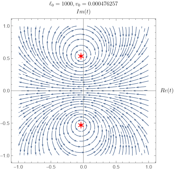
Refer to caption
Refer to caption
Refer to caption
Refer to caption
Figure 25: The RG flow projected onto the subspace of one complex four-fermion coupling in the spin anti-symmetric d-wave pairing channel with Cooper-pair wave function given in Eq. ( \theequation@prefix214) for Nc=2N_{c}=2, Nf=1N_{f}=1, Δ/Λ=108\Delta/\Lambda=10^{8} and ε/Λ=10−10\varepsilon/\Lambda=10^{-10} with ℓ0=\ell_{0}= 103,104,105,10610^{3},10^{4},10^{5},10^{6} from top left to bottom right. With increasing ℓ0\ell_{0} (decreasing v0​(0)v_{0}(0)), the pair of complex quasi-fixed points approach to the real axis, creating a bottleneck region in the real axis.

The existence of channels in which the quasi-fixed points arise away from the real axis suggests that a Hermitian theory eventually flows toward a superconducting fixed point at low energies. When the nesting angle is small, we expect a weaker superconducting instability as the pairing interaction generated from the spin fluctuations is weak. Indeed, the non-Hermitian quasi-fixed points get closer to the space of Hermitian theories as vv decreases. In Fig. 25, we plot the projected RG flow around the non-Hermitian quasi fixed point in the spin anti-symmetric d-wave channel for different values of vv. With decreasing vv, the quasi-fixed points approach the real axis, creating a bottleneck in the RG flow of Hermitian theories. The bottleneck creates a large window of length scale in which the theory exhibits an approximate scale invariance before the system eventually becomes superconducting in the low energy limit.

Our next task is to understand how Hermitian theories undergo superconducting instabilities at low energies. We can not use Eq. ( \theequation@prefix217) to describe the actual superconducting instability because the full RG flow does not stay within the one-dimensional subspace spanned by Eq. ( \theequation@prefix213). The RG flow that is projected to a fixed channel does not capture how the Cooper pair wavefunction evolves under the RG flow. In particular, the dilatation term in the beta functional continuously push electrons from the hot region to the cold region under the RG flow, which broadens the width of the pair wavefunction relative to the width of the hot spot region4343 43 This reflects the fact that more and more electrons are decoupled from spin fluctuations as the low-energy limit is taken.. Therefore, we go back to the full beta functional to address superconducting instability.

VIII Superconducting instability

• Theories whose bare four-fermion interactions are attractive and stronger than the interaction mediated by the critical spin fluctuations develop superconducting instabilities via the conventional BCS mechanism in which the nearby non-Fermi liquid fixed point plays little role. • Theories whose bare four-fermion interactions are not strongly attractive in any channel necessarily flow through the bottleneck region controlled by the non-Fermi liquid fixed point. It creates a window of energy scale for quasi-universal scaling, where the energy window increases with decreasing bare nesting angle. • The superconducting transition temperature and the pairing wavefunction of those theories that go through the bottleneck region are determined from the bare nesting angle that sets the distance of the bare theory from the non-Fermi liquid fixed point.

In this section, we study superconducting instability by solving the beta functional for the four-fermion coupling function in the pairing channel with a fixed nesting angle. This is justified because the theory undergoes a superconducting instability before the nesting angle changes appreciably in the small vv limit, as will be shown later. Since we already know that there is no Hermitian fixed point with v≠0v\neq 0, for the purpose of understanding superconductivity, it is simpler to use the beta functional for the coupling function defined in the space of physical momentum. The way superconductivity emerges at low energies can be understood from the solution of the beta functional for the four-fermion coupling function. Since λ2​P​P​(p−pk−k)V;(±),(sd){\lambda}^{V;(\pm),\begin{pmatrix}s\\ d\end{pmatrix}}_{2PP\begin{pmatrix}p&-p\\ k&-k\end{pmatrix}} is sensitive to the boson propagator at large momenta, only the net two-body interaction function defined in Eq. ( \theequation@prefix193) can be determined within the low-energy effective field theory. Nonetheless, we can still understand superconducting instabilities by solving Eq. ( \theequation@prefix192) for λ2​P​P​(p−pk−k)V;(±),(sd){\lambda}^{V;(\pm),\begin{pmatrix}s\\ d\end{pmatrix}}_{2PP\begin{pmatrix}p&-p\\ k&-k\end{pmatrix}}, assuming that the boson propagator takes the form of Eq. ( \theequation@prefix126) at all momenta. Although 𝖣μ​(q,k)\mathsf{D}_{\mu}(q;k) in Eq. ( \theequation@prefix126) and λ2​P​P​(p−pk−k)V;(±),(sd){\lambda}^{V;(\pm),\begin{pmatrix}s\\ d\end{pmatrix}}_{2PP\begin{pmatrix}p&-p\\ k&-k\end{pmatrix}} obtained from Eq. ( \theequation@prefix192) are not individually reliable at large momenta, the combination in Eq. ( \theequation@prefix193) is insensitive to the unknown UV physics. In particular, if the net two-body interaction diverges due to a superconducting instability, so does λ2​P​P​(p−pk−k)V;(±),(sd){\lambda}^{V;(\pm),\begin{pmatrix}s\\ d\end{pmatrix}}_{2PP\begin{pmatrix}p&-p\\ k&-k\end{pmatrix}} because Eq. ( \theequation@prefix126) is regular. Therefore, we directly solve the beta functional in Eq. ( \theequation@prefix192). The manner superconductivity arises crucially depends on whether the bare coupling function has any channel with attractive interaction which is stronger than the interaction mediated by the spin fluctuations or not Kohn and Luttinger 1965. Therefore, discussion on superconductivity is divided into two parts.

VIII-(aa)  Attractive bare interaction

If the bare interaction is attractive in any channel with its strength greater than w=v/cw=v/c, Eq. ( \theequation@prefix192) is dominated by the BCS term that is quadratic in the four-fermion coupling. In this case, Eq. ( \theequation@prefix192) is well approximated by

∂∂ℓ​λ2​P​P​(p−pk−k)V;(±),(sd)=−λ2​P​P​(p−pk−k)V;(±),(sd)−14​π​∫d​q2​π​μ​λ2​P​P​(p−pq−q)V;(±),(sd)​λ2​P​P​(q−qk−k)V;(±),(sd).\displaystyle\frac{\partial}{\partial\ell}{\lambda}^{V;(\pm),\begin{pmatrix}s\\ d\end{pmatrix}}_{2PP\begin{pmatrix}p&-p\\ k&-k\end{pmatrix}}=-{\lambda}^{V;(\pm),\begin{pmatrix}s\\ d\end{pmatrix}}_{2PP\begin{pmatrix}p&-p\\ k&-k\end{pmatrix}}-\frac{1}{4\pi}\int\frac{\mathrm{d}q}{2\pi\mu}\lambda^{V;(\pm),\begin{pmatrix}s\\ d\end{pmatrix}}_{2PP\begin{pmatrix}p&-p\\ q&-q\end{pmatrix}}\lambda^{V;(\pm),\begin{pmatrix}s\\ d\end{pmatrix}}_{2PP\begin{pmatrix}q&-q\\ k&-k\end{pmatrix}}. ( \theequation@prefix222)

The first term on the right hand side reflects the fact that the four-fermion coupling is irrelevant by power-counting under the scaling in which all components of momentum are scaled. The flip side of the scaling is the scale dependent measure d​q2​π​μ\frac{\mathrm{d}q}{2\pi\mu} in the second term. It describes the BCS process in which Cooper pairs are scattered to intermediate states on the Fermi surface. The volume of the phase space for virtual Cooper pairs measured in the unit of the running energy scale μ=Λ​e−ℓ\mu=\Lambda e^{-\ell} increases with decreasing energy. The enhancement from the phase space volume compensates the suppression from the power-counting, effectively promoting the four-fermion coupling to a marginal coupling as expected. This can be easily seen by absorbing a factor of eℓe^{\ell} into the coupling to write the beta functional as

∂∂ℓ(eℓλ2​P​P​(p−pk−k)V;(±),(sd))=−14​π∫d​q2​π​Λ(eℓλ2​P​P​(p−pq−q)V;(±),(sd))(eℓλ2​P​P​(q−qk−k)V;(±),(sd)).\displaystyle\frac{\partial}{\partial\ell}\left(e^{\ell}{\lambda}^{V;(\pm),\begin{pmatrix}s\\ d\end{pmatrix}}_{2PP\begin{pmatrix}p&-p\\ k&-k\end{pmatrix}}\right)=-\frac{1}{4\pi}\int\frac{\mathrm{d}q}{2\pi\Lambda}\left(e^{\ell}\lambda^{V;(\pm),\begin{pmatrix}s\\ d\end{pmatrix}}_{2PP\begin{pmatrix}p&-p\\ q&-q\end{pmatrix}}\right)\left(e^{\ell}\lambda^{V;(\pm),\begin{pmatrix}s\\ d\end{pmatrix}}_{2PP\begin{pmatrix}q&-q\\ k&-k\end{pmatrix}}\right). ( \theequation@prefix223)

Its solution is given by

λV;(±),(sd)​(ℓ)=e−ℓ​λV;(±),(sd)​(0)​[1+ℓ4​π​λV;(±),(sd)​(0)]−1.\displaystyle{\lambda}^{V;(\pm),\begin{pmatrix}s\\ d\end{pmatrix}}(\ell)=e^{-\ell}{\lambda}^{V;(\pm),\begin{pmatrix}s\\ d\end{pmatrix}}(0)\left[1+\frac{\ell}{4\pi}{\lambda}^{V;(\pm),\begin{pmatrix}s\\ d\end{pmatrix}}(0)\right]^{-1}. ( \theequation@prefix224)

Here λV;(±),(sd){\lambda}^{V;(\pm),\begin{pmatrix}s\\ d\end{pmatrix}} is viewed as a matrix defined in the space of momentum. In this expression, the matrix multiplications are defined with the measure (A​B)p,k=∫d​q2​π​Λ​Ap​q​Bq​k(AB)_{p,k}=\int\frac{\mathrm{d}q}{2\pi\Lambda}A_{pq}B_{qk}. If λV​(0){\lambda}^{V}(0) has any channel with negative eigenvalue, the four-fermion coupling blows up around scale ℓc∼4​π|E|\ell_{c}\sim\frac{4\pi}{|E|}, where E<0E<0 is the most negative eigenvalue of the bare coupling. For |E|>w|E|>w, ℓc<1/w≪ℓ0\ell_{c}<1/w\ll\ell_{0}, and the flow of vv is negligible between ℓ=0\ell=0 and ℓc\ell_{c}. When the bare interaction is attractive and stronger than ww, the superconducting transition temperature and the pairing wavefunction are sensitive to the bare four-fermion coupling. In this case, gapless spin fluctuations have little effect on superconductivity, and the manner in which superconductivity emerges is not universal.

VIII-(bb)  Repulsive bare interaction

Theories in which the bare coupling is not strongly attractive in any channel are more interesting in that the emergence of superconductivity is governed by the universal physics associated with the nearby non-Fermi liquid fixed point. This is because those theories necessarily flow through the bottleneck region where the RG flow is constricted. To see this, we view λ2​P​PV\lambda^{V}_{2PP} in Eq. ( \theequation@prefix186) as a matrix and decompose it as λ2​P​PV=∑iλi​|i⟩​⟨i|{\lambda}^{V}_{2PP}=\sum_{i}{\lambda}_{i}|i\rangle\langle i|. Here, the channel indices ((±),(sd)(\pm),\begin{pmatrix}s\\ d\end{pmatrix}) are dropped to avoid clutter in notation. |i⟩|i\rangle’s (⟨i|\langle i|’s) represent normalized column (row) eigenvectors that diagonalize the four fermion coupling function, and λi{\lambda}_{i}’s represent the eigenvalues. Eigenvalues and eigenvectors obey the flow equations given by

∂∂ℓ​λi=\displaystyle\frac{\partial}{\partial\ell}{\lambda}_{i}= −λi−2​⟨i|η|i⟩μ​λi−14​π​⟨i|(λ′)2|i⟩μ,\displaystyle-{\lambda}_{i}-2\langle i|\eta|i\rangle_{\mu}{\lambda}_{i}-\frac{1}{4\pi}\langle i|(\lambda^{\prime})^{2}|i\rangle_{\mu}, ( \theequation@prefix225)
∂|i⟩∂ℓ=\displaystyle\frac{\partial|i\rangle}{\partial\ell}= −∑j≠i(λi+λj)​(⟨j|η|i⟩μ−α(n)4​π​⟨j|𝖣V|i⟩μ)+(α(n))24​π​⟨j​|(𝖣V)2|​i⟩μλi−λj|j⟩.\displaystyle-\sum_{j\neq i}\frac{(\lambda_{i}+\lambda_{j})\left(\langle j|\eta|i\rangle_{\mu}-\frac{\alpha^{(n)}}{4\pi}\langle j|\mathsf{D}^{V}|i\rangle_{\mu}\right)+\frac{(\alpha^{(n)})^{2}}{4\pi}\langle j|\left(\mathsf{D}^{V}\right)^{2}|i\rangle_{\mu}}{\lambda_{i}-\lambda_{j}}|j\rangle.

Here, ⟨i|C|j⟩μ≡∫d​k​d​p(2​π​μ)2​fi,k∗​Ck​p​fj,p\langle i|C|j\rangle_{\mu}\equiv\int\frac{\mathrm{d}k\mathrm{d}p}{(2\pi\mu)^{2}}f_{i,k}^{*}C_{kp}f_{j,p} with fi,kf_{i,k} representing the ii-th eigenvector written in the momentum space. η\eta is a diagonal matrix with ηp,k=2​π​μ​δ​(p−k)​ηp\eta_{p,k}=2\pi\mu\delta(p-k)\eta_{p}. λ′(±),(sd)(p−pq−q)\lambda^{{}^{\prime}(\pm),\begin{pmatrix}s\\ d\end{pmatrix}}_{\begin{pmatrix}p&-p\\ q&-q\end{pmatrix}} is defined in Eq. ( \theequation@prefix193) and Dp,kV≡𝖣μ​(p,k)VF,p​VF,kD^{V}_{p,k}\equiv\frac{\mathsf{D}_{\mu}(p;k)}{\sqrt{V_{F,p}V_{F,k}}}. Since η\eta and (λ′)2(\lambda^{\prime})^{2} are non-negative matrices, d​λid​ℓ≤0\frac{d{\lambda}_{i}}{d\ell}\leq 0 for λi≥0\lambda_{i}\geq 0. This means that theories with repulsive couplings flow toward λi=0\lambda_{i}=0 at low energies. In the small vv limit, theories with bare repulsive couplings flow to the fixed point at λi=0\lambda_{i}=0. For v≠0v\neq 0, λi=0\lambda_{i}=0 is no longer a fixed point. Since ∂λi∂ℓ<0\frac{\partial{\lambda}_{i}}{\partial\ell}<0 for λi≥0\lambda_{i}\geq 0, all theories with v≠0v\neq 0 develop at least one channel with attractive interactions at sufficiently low energies4444 44 This is expected from the absence of Hermitian quasi-fixed points with v≠0v\neq 0.. Although λ=0\lambda=0 is not a fixed point, it still acts as an approximate focal point in the space of theories because at λ=0\lambda=0 the beta functional is proportional to 𝖣μ2\mathsf{D}_{\mu}^{2} whose eigenvalues are order of w2w^{2}. In the small vv limit, the slow RG speed near λ=0\lambda=0 creates a bottleneck region in which a theory spends a long RG ‘time’. Consequently, bare theories with O⁡(1)O(1) repulsive interactions are naturally attracted to the region with |λi|≤w|\lambda_{i}|\leq w at scale ℓ∗∼w−1\ell^{*}\sim w^{-1} before they become negative. For v≠0v\neq 0, there is no perfect focusing of the RG flow. Nonetheless, theories spend longer RG time in the bottleneck region as vv decreases. This makes the theory within the bottleneck an approximate attractor of UV theoriesZumbach 1993; Wang et al. 2017c. Once theories are attracted to the bottleneck region, the superconducting transition temperature is determined by the RG time that is needed for theories to pass through it. In this section, we examine how superconductivity emerges in a theory that is within the bottleneck region with λ≈0\lambda\approx 0 at a scale ℓ∗\ell^{*}.

To remove the explicit scale dependence in the measure of the momentum integration of the beta functional, we consider

λ¯2​P​P​(p−pk−k)V;(±),(sd)=eℓ​λ2​P​P​(p−pk−k)V;(±),(sd).\displaystyle\bar{\lambda}^{V;(\pm),\begin{pmatrix}s\\ d\end{pmatrix}}_{2PP\begin{pmatrix}p&-p\\ k&-k\end{pmatrix}}=e^{\ell}\lambda^{V;(\pm),\begin{pmatrix}s\\ d\end{pmatrix}}_{2PP\begin{pmatrix}p&-p\\ k&-k\end{pmatrix}}. ( \theequation@prefix226)

Its beta functional reads

∂∂ℓ​λ¯2​P​P​(p−pk−k)V;(±),(sd)=−(ηk+ηp)​λ¯2​P​P​(p−pk−k)V;(±),(sd)\displaystyle\frac{\partial}{\partial\ell}\bar{\lambda}^{V;(\pm),\begin{pmatrix}s\\ d\end{pmatrix}}_{2PP\begin{pmatrix}p&-p\\ k&-k\end{pmatrix}}=-\left(\eta_{k}+\eta_{p}\right)\bar{\lambda}^{V;(\pm),\begin{pmatrix}s\\ d\end{pmatrix}}_{2PP\begin{pmatrix}p&-p\\ k&-k\end{pmatrix}}
−14​π∫d​q2​π​Λ[λ¯2​P​P​(p−pq−q)V;(±),(sd)−2NfYP​P(±)1(sd)eℓ​𝖣Λ​e−ℓ​(p,q)VF,p​VF,q][λ¯2​P​P​(q−qk−k)V;(±),(sd)−2NfYP​P(±)1(sd)eℓ​𝖣Λ​e−ℓ​(q,k)VF,q​VF,k].\displaystyle-\frac{1}{4\pi}\int\frac{\mathrm{d}q}{2\pi\Lambda}\left[\bar{\lambda}^{V;(\pm),\begin{pmatrix}s\\ d\end{pmatrix}}_{2PP\begin{pmatrix}p&-p\\ q&-q\end{pmatrix}}-\frac{2}{N_{f}}Y_{PP}^{(\pm)}1^{\begin{pmatrix}s\\ d\end{pmatrix}}\frac{e^{\ell}{\mathsf{D}}_{\Lambda e^{-\ell}}(p;q)}{\sqrt{V_{F,p}V_{F,q}}}\right]\left[\bar{\lambda}^{V;(\pm),\begin{pmatrix}s\\ d\end{pmatrix}}_{2PP\begin{pmatrix}q&-q\\ k&-k\end{pmatrix}}-\frac{2}{N_{f}}Y_{PP}^{(\pm)}1^{\begin{pmatrix}s\\ d\end{pmatrix}}\frac{e^{\ell}{\mathsf{D}}_{\Lambda e^{-\ell}}(q;k)}{\sqrt{V_{F,q}V_{F,k}}}\right]. ( \theequation@prefix227)

Here, 𝖣μ​(q,k){\mathsf{D}}_{\mu}(q;k) is defined in Eq. ( \theequation@prefix126). A theory that is at the bottleneck point at scale ℓ∗\ell^{*} corresponds to the ‘initial’ condition

λ¯2​P​P​(p−pk−k)V;(±),(sd)​(ℓ∗)=0.\displaystyle\bar{\lambda}^{V;(\pm),\begin{pmatrix}s\\ d\end{pmatrix}}_{2PP\begin{pmatrix}p&-p\\ k&-k\end{pmatrix}}(\ell^{*})=0. ( \theequation@prefix228)

In the following, we focus on the d-wave and spin anti-symmetric sector in which the attractive interaction is strongestScalapino et al. 1986; PhysRevB.81.224505. At energy scales that are not too smaller than Λ∗=Λ​e−ℓ∗\Lambda^{*}=\Lambda e^{-\ell^{*}}, we can ignore λ¯2​P​PV\bar{\lambda}_{2PP}^{V} on the right hand side of Eq. ( \theequation@prefix227). As the energy scale is lowered, the spin fluctuations generate attractive interaction which, in turn, accelerates the flow of λ¯2​P​PV\bar{\lambda}_{2PP}^{V}4545 45 This follows from the fact that the largest eigenvalue of 𝖣μ{\mathsf{D}}_{\mu} is positive and YP​P(−)​1(d)=2​(1+1Nc)>0Y_{PP}^{(-)}1^{\begin{pmatrix}d\end{pmatrix}}=2\left(1+\frac{1}{N_{c}}\right)>0. . At sufficiently low energies, the magnitude of λ¯2​P​PV\bar{\lambda}_{2PP}^{V} surpasses that of −2Nf​YP​P(±)​1(sd)​eℓ​𝖣Λ​e−ℓ​(p,q)VF,p​VF,q-\frac{2}{N_{f}}Y_{PP}^{(\pm)}1^{\begin{pmatrix}s\\ d\end{pmatrix}}\frac{e^{\ell}{\mathsf{D}}_{\Lambda e^{-\ell}}(p;q)}{\sqrt{V_{F,p}V_{F,q}}} in Eq. ( \theequation@prefix227). As the four-fermion coupling becomes stronger than the attractive interaction generated by spin fluctuations at low energies, the further growth of the four-fermion coupling is dominated by the BCS process. We denote this crossover scale as ℓ1\ell_{1}. Since the beta function is dominated by different terms below and above the crossover scales, we write the approximate solution of the beta functional as

λ¯2​P​PV={λ¯Ifor ℓ<ℓ1λ¯I​Ifor ℓ>ℓ1.\displaystyle\bar{\lambda}_{2PP}^{V}=\left\{\begin{array}[]{cl}\bar{\lambda}_{I}&~~~\mbox{for $\ell<\ell_{1}$}\\ \bar{\lambda}_{II}&~~~\mbox{for $\ell>\ell_{1}$}\end{array}\right..

For ℓ<ℓ1\ell<\ell_{1}, the RG flow is approximated by

∂∂ℓλ¯I,(p−pk−k)(−),(d)≈−14​π(2​YP​P(−)Nf)2∫d​q2​π​Λeℓ​𝖣Λ​e−ℓ​(p,q)VF,p​VF,qeℓ​𝖣Λ​e−ℓ​(q,k)VF,q​VF,k.\displaystyle\frac{\partial}{\partial\ell}\bar{\lambda}^{(-),\begin{pmatrix}d\end{pmatrix}}_{I,\begin{pmatrix}p&-p\\ k&-k\end{pmatrix}}\approx-\frac{1}{4\pi}\left(\frac{2Y_{PP}^{(-)}}{N_{f}}\right)^{2}\int\frac{\mathrm{d}q}{2\pi\Lambda}\frac{e^{\ell}{\mathsf{D}}_{\Lambda e^{-\ell}}(p;q)}{\sqrt{V_{F,p}V_{F,q}}}\frac{e^{\ell}{\mathsf{D}}_{\Lambda e^{-\ell}}(q;k)}{\sqrt{V_{F,q}V_{F,k}}}. ( \theequation@prefix232)

It describes the process in which the four-fermion coupling is generated from gapless spin fluctuations. The contribution of the anomalous dimension can be also ignored because λ2​P​PV\lambda_{2PP}^{V} is small. The solution of Eq. ( \theequation@prefix232) is written as

λ¯I,(p−pk−k)(−),(d)​(ℓ)\displaystyle\bar{\lambda}^{(-),\begin{pmatrix}d\end{pmatrix}}_{I,\begin{pmatrix}p&-p\\ k&-k\end{pmatrix}}(\ell) =\displaystyle= −14​π(2​YP​P(−)Nf)2∫ℓ∗ℓdℓ′1VF,p​VF,k×\displaystyle-\frac{1}{4\pi}\left(\frac{2Y_{PP}^{(-)}}{N_{f}}\right)^{2}\int_{\ell^{*}}^{\ell}d\ell^{\prime}\frac{1}{\sqrt{V_{F,p}V_{F,k}}}\times ( \theequation@prefix233)
∫d​q2​π​VF,q​gp,q2​gq,k2​Λ[μ′+c​|p−q|μ′+c​|vp​p+vq​q|μ′]​[μ′+c​|q−k|μ′+c​|vq​q+vk​k|μ′],\displaystyle\int\frac{dq}{2\pi V_{F,q}}\frac{g_{p,q}^{2}g_{q,k}^{2}\Lambda}{\left[\mu^{\prime}+c\left|p-q\right|_{\mu^{\prime}}+c\left|v_{p}p+v_{q}q\right|_{\mu^{\prime}}\right]\left[\mu^{\prime}+c\left|q-k\right|_{\mu^{\prime}}+c\left|v_{q}q+v_{k}k\right|_{\mu^{\prime}}\right]},

where μ′=Λ​e−ℓ′\mu^{\prime}=\Lambda e^{-\ell^{\prime}}, and all coupling functions on the right hand side of the equation are evaluated at scale ℓ′\ell^{\prime}. Let us denote the most negative eigenvalue and the associated eigenvector of λ¯I​(ℓ)\bar{\lambda}_{I}(\ell) as E0​(ℓ)E_{0}(\ell) and Fk​(ℓ)F_{k}(\ell), respectively. The crossover scale ℓ1\ell_{1} is determined from the condition that E0​(ℓ)E_{0}(\ell) becomes comparable to the spin fluctuation-induced interaction projected onto Fk​(ℓ)F_{k}(\ell),

E0​(ℓ1)∼2Nf​YP​P(−)​⟨eℓ1​𝖣Λ​e−ℓ1​(p,k)VF,p​VF,k⟩F,\displaystyle E_{0}(\ell_{1})\sim\frac{2}{N_{f}}Y_{PP}^{(-)}\left\langle\frac{e^{\ell_{1}}{\mathsf{D}}_{\Lambda e^{-\ell_{1}}}(p;k)}{\sqrt{V_{F,p}V_{F,k}}}\right\rangle_{F}, ( \theequation@prefix234)

where ⟨eℓ1​𝖣Λ​e−ℓ1​(p,k)VF,p​VF,k⟩F=∫d​p​d​k(2​π​Λ)2​eℓ1​𝖣Λ​e−ℓ1​(p,k)VF,p​VF,k​Fp∗​(ℓ1)​Fk​(ℓ1)\left\langle\frac{e^{\ell_{1}}{\mathsf{D}}_{\Lambda e^{-\ell_{1}}}(p;k)}{\sqrt{V_{F,p}V_{F,k}}}\right\rangle_{F}=\int\frac{dpdk}{(2\pi\Lambda)^{2}}\frac{e^{\ell_{1}}{\mathsf{D}}_{\Lambda e^{-\ell_{1}}}(p;k)}{\sqrt{V_{F,p}V_{F,k}}}F_{p}^{*}(\ell_{1})F_{k}(\ell_{1}). To the leading order in vv, the four-fermion coupling function generated by the Yukawa coupling in Eq. ( \theequation@prefix233) decays as 1/|p−k|1/|p-k| at large momenta up to a logarithmic correction. The slow decay of the large-angle scatterings give rise to inter-patch couplings that invalidates the patch description.

Since it is difficult to analytically compute the eigenvector of λ¯I,(p−pk−k)(−),(d)​(ℓ)\bar{\lambda}^{(-),\begin{pmatrix}d\end{pmatrix}}_{I,\begin{pmatrix}p&-p\\ k&-k\end{pmatrix}}(\ell), we first estimate the crossover scale using a simple Ansatz. At energy scale Λ∗\Lambda^{*}, electrons within the range of momentum |k|<Λ∗/(v​c)|k|<\Lambda^{*}/(vc) are strongly coupled with spin fluctuations. Therefore, we consider a Cooper pair wavefunction whose width is order of Λ∗/(v​c)\Lambda^{*}/(vc) in the momentum space,

fk=(2​π​v​cΛ∗)1/2​Θ​(12−v​c​|k|Λ∗).f_{k}=\left(\frac{2\pi vc}{\Lambda^{*}}\right)^{1/2}\Theta\left(\frac{1}{2}-\frac{vc\left|k\right|}{\Lambda^{*}}\right). ( \theequation@prefix235)

The expectation value of eℓ​𝖣μVF​VF\frac{e^{\ell}\mathsf{D}_{\mu}}{\sqrt{V_{F}}\sqrt{V_{F}}} for this Ansatz is written as

⟨eℓ​𝖣μVF​VF⟩\displaystyle\left\langle\frac{e^{\ell}\mathsf{D}_{\mu}}{\sqrt{V_{F}}\sqrt{V_{F}}}\right\rangle =∫d​k​d​p(2​π​Λ)2​gk​p​(ℓ)2VF,k​(ℓ)​VF,p​(ℓ)​ΛΛ​e−ℓ+c​|k−p|+c​v​|k+p|​fk∗​(ℓ)​fp​(ℓ),\displaystyle=\int\frac{\mathrm{d}k\mathrm{d}p}{(2\pi\Lambda)^{2}}\frac{g_{kp}(\ell)^{2}}{\sqrt{V_{F,k}(\ell)V_{F,p}(\ell)}}\frac{\Lambda}{\Lambda e^{-\ell}+c\left|k-p\right|+cv\left|k+p\right|}f^{*}_{k}(\ell)f_{p}(\ell), ( \theequation@prefix236)

where

gk,p​(ℓ)=gk,p​(0)​(μ max​{μ,2​v​|k+p|,2​v​c​|k|,2​v​c​|p|})α0​(ℓ0),VF,k​(ℓ)=(μmax​{μ,4​v​|k|})α1​(ℓ0)/2g_{k,p}(\ell)=g_{k,p}(0)\left(\frac{\mu}{\text{ max}\{\mu,2v\left|k+p\right|,2vc\left|k\right|,2vc\left|p\right|\}}\right)^{\alpha_{0}(\ell_{0})},~~V_{F,k}(\ell)=\left(\frac{\mu}{\text{max}\{\mu,4v|k|\}}\right)^{\alpha_{1}(\ell_{0})/2} ( \theequation@prefix237)

with μ=Λ​e−ℓ\mu=\Lambda e^{-\ell} and α0\alpha_{0}, α1\alpha_{1} defined in Eq. ( \theequation@prefix157). To simplify the computation of Eq. ( \theequation@prefix236), we first use a few assumptions, and later justify them from the solution. First, we assume that the Yukawa coupling function does not change significantly as a function of ℓ\ell for ℓ∗<ℓ<ℓ1\ell^{*}<\ell<\ell_{1} :

gk,p​(ℓ1)gk,p​(ℓ∗)∼1,\frac{g_{k,p}(\ell_{1})}{g_{k,p}(\ell^{*})}\sim 1, ( \theequation@prefix238)

where ℓ∗\ell^{*} is the scale at which the theory is in the bottleneck region and ℓ1\ell_{1} is the crossover scale. If Eq. ( \theequation@prefix238) is satisfied, the scale dependence of VF,k​(ℓ)V_{F,k}(\ell) can be also ignored in ℓ∗<ℓ<ℓ1\ell^{*}<\ell<\ell_{1} because α1≪α0\alpha_{1}\ll\alpha_{0} in the small vv limit. Second, we assume that the coupling functions are almost constant within the support of fkf_{k} :

VF,k​(ℓ)≈1,gk,p​(ℓ)≈g0​(ℓ)V_{F,k}(\ell)\approx 1,\quad g_{k,p}(\ell)\approx g_{0}(\ell) ( \theequation@prefix239)

for |k|<Λ∗/(v​c)|k|<\Lambda^{*}/(vc) and ℓ∗<ℓ<ℓ1\ell^{*}<\ell<\ell_{1}. Finally, we assume that the crossover occurs at an energy that is much smaller than Λ∗\Lambda^{*},

ℓ1≫ℓ∗.\ell_{1}\gg\ell^{*}. ( \theequation@prefix240)

These assumptions allow us to approximate ( \theequation@prefix236) as

⟨eℓ​𝖣μVF​VF⟩≈g0​(ℓ∗)2​∫d​k​d​p(2​π​Λ)2​Λc​|k−p|+c​v​|k+p|​fk∗​(ℓ)​fp​(ℓ)\left\langle\frac{e^{\ell}\mathsf{D}_{\mu}}{\sqrt{V_{F}}\sqrt{V_{F}}}\right\rangle\approx g_{0}(\ell^{*})^{2}\int\frac{\mathrm{d}k\mathrm{d}p}{(2\pi\Lambda)^{2}}\frac{\Lambda}{c\left|k-p\right|+cv\left|k+p\right|}f^{*}_{k}(\ell)f_{p}(\ell) ( \theequation@prefix241)

for ℓ∗<ℓ<ℓ1\ell^{*}<\ell<\ell_{1}. The direct integrations over the momenta gives

⟨eℓ​𝖣μVF​VF⟩≈g0​(ℓ∗)2π​c​log⁡(1v)=w0​(ℓ∗)2​log⁡(1v).\left\langle\frac{e^{\ell}\mathsf{D}_{\mu}}{\sqrt{V_{F}}\sqrt{V_{F}}}\right\rangle\approx\frac{g_{0}(\ell^{*})^{2}}{\pi c}\log\left(\frac{1}{v}\right)=\frac{w_{0}(\ell^{*})}{2}\log\left(\frac{1}{v}\right). ( \theequation@prefix242)

Eq. ( \theequation@prefix242) is largely independent of ℓ\ell4646 46 While eℓ​𝖣Λ​e−ℓ​(p,k)VF,p​VF,k\frac{e^{\ell}{\mathsf{D}}_{\Lambda e^{-\ell}}(p;k)}{\sqrt{V_{F,p}V_{F,k}}} at the hot spot (p=k=0p=k=0) increases without a bound with increasing ℓ\ell, its eigenvalues remain bounded at all ℓ\ell. In particular, ∫−kFkFd​p2​π​Λ​∫−kFkFd​k2​π​Λ​fp∗​Λc​|k−p|+c​v0​|k+p|​fk\int_{-k_{F}}^{k_{F}}\frac{\mathrm{d}p}{2\pi\Lambda}\int_{-k_{F}}^{k_{F}}\frac{\mathrm{d}k}{2\pi\Lambda}f_{p}^{*}~\frac{\Lambda}{c\left|k-p\right|+cv_{0}\left|k+p\right|}~f_{k} is finite for all square integrable functions fkf_{k}. . On the other hand, E0​(ℓ)E_{0}(\ell) grows linearly in ℓ\ell as

E0​(ℓ)∼−14​π​Nf2​(YP​P(−))2​(ℓ−ℓ∗)​⟨eℓ​𝖣μVF​VF⟩f2∼−14​π​Nf2​(YP​P(−))2​(ℓ−ℓ∗)​w2​log2⁡(1v).\displaystyle E_{0}(\ell)\sim-\frac{1}{4\pi N_{f}^{2}}\left(Y_{PP}^{(-)}\right)^{2}(\ell-\ell^{*})\left\langle\frac{e^{\ell}\mathsf{D}_{\mu}}{\sqrt{V_{F}}\sqrt{V_{F}}}\right\rangle_{f}^{2}\sim-\frac{1}{4\pi N_{f}^{2}}\left(Y_{PP}^{(-)}\right)^{2}(\ell-\ell^{*})w^{2}\log^{2}\left(\frac{1}{v}\right). ( \theequation@prefix243)

Inserting Eqs. ( \theequation@prefix242)-( \theequation@prefix243) to Eq. ( \theequation@prefix234), we obtain the crossover scale to be

ℓ1∼ℓ∗+2​π​Nf(1+1Nc)​1w​log⁡(1/v),\displaystyle\ell_{1}\sim\ell^{*}+\frac{2\pi N_{f}}{\left(1+\frac{1}{N_{c}}\right)}\frac{1}{w\log(1/v)}, ( \theequation@prefix244)

and the strength of the four-fermion coupling at the crossover scale is

E0​(ℓ1)∼−2Nf​(1+1Nc)​w​log⁡(1v).E_{0}(\ell_{1})\sim-\frac{2}{N_{f}}\left(1+\frac{1}{N_{c}}\right)w\log\left(\frac{1}{v}\right). ( \theequation@prefix245)

The consistency of the assumptions used in Eqs. ( \theequation@prefix238) -( \theequation@prefix240) can be checked4747 47 Eq. ( \theequation@prefix240) directly follows from Eq. ( \theequation@prefix244). With α0\alpha_{0} and cc expressed in terms of vv as α0​(v)=v​log⁡(1/v)2​π​Nc​Nf\alpha_{0}(v)=\frac{\sqrt{v\log(1/v)}}{\sqrt{2}\pi\sqrt{N_{c}N_{f}}}, c⁡(v)=v8​Nc​Nf​log⁡(1v)c(v)=\sqrt{\frac{v}{8N_{c}N_{f}}\log\left(\frac{1}{v}\right)}, Eq. ( \theequation@prefix238) becomes gk,p​(ℓ1)gk,p​(ℓ∗)∼e−α0​(ℓ0)​(ℓ1−ℓ∗)∼e−12​(Nc+1)∼1\frac{g_{k,p}(\ell_{1})}{g_{k,p}(\ell^{*})}\sim e^{-\alpha_{0}(\ell_{0})(\ell_{1}-\ell^{*})}\sim e^{-\frac{1}{2(N_{c}+1)}}\sim 1. For Nc=2,Nf=1N_{c}=2,N_{f}=1, g⁡(ℓ1)/g⁡(ℓ∗)≈0.846482g(\ell_{1})/g(\ell^{*})\approx 0.846482. Eq. ( \theequation@prefix239) for the diagonal Yukawa coupling can be checked from gΛ∗v​c​(ℓ1)g0​(ℓ1)∼(Λ​e−ℓ1Λ∗)α0=e−α0​(ℓ1−ℓ∗)∼1\frac{g_{\frac{\Lambda^{*}}{vc}}(\ell_{1})}{g_{0}(\ell_{1})}\sim\left(\frac{\Lambda e^{-\ell_{1}}}{\Lambda^{*}}\right)^{\alpha_{0}}=e^{-\alpha_{0}(\ell_{1}-\ell^{*})}\sim 1. Similarly, Eq. ( \theequation@prefix239) for the off-diagonal Yukawa coupling and VF,kV_{F,k} follow. .

We confirm this estimation of the crossover scale by numerically diagonalizing Eq. ( \theequation@prefix233). Fig. 26( a ) shows the numerical results for the most negative eigenvalue of λ¯I,(p−pk−k)(−),(d)​(ℓ)\bar{\lambda}^{(-),\begin{pmatrix}d\end{pmatrix}}_{I,\begin{pmatrix}p&-p\\ k&-k\end{pmatrix}}(\ell) and the expectation value of eℓ1​𝖣Λ​e−ℓ1​(p,k)VF,p​VF,k\frac{e^{\ell_{1}}{\mathsf{D}}_{\Lambda e^{-\ell_{1}}}(p;k)}{\sqrt{V_{F,p}V_{F,k}}} evaluated for the corresponding eigenvector. While the magnitude of the former increases more or less linearly in ℓ−ℓ∗\ell-\ell^{*}, the expectation value of the latter is largely constant, as expected. This results in the crossover at a scale ℓ1\ell_{1}. At the crossover scale, the eigenvector shown in Fig. 26( b ) is peaked at the hot spot but its support is extended to Λ∗/(v​c)\Lambda^{*}/(vc). As is expected, the crossover scale increases with decreasing vv (or increasing ℓ0\ell_{0}) as is shown in Fig. 26( c ).

(a{\color[rgb]{0,0,1}a})
(b{\color[rgb]{0,0,1}b})
(c{\color[rgb]{0,0,1}c})
Figure 26: Numerical results for the crossover scale and the Cooper pair wavefunction. (a) The solid and dashed lines denote the most negative eigenvalue of Eq. ( \theequation@prefix233) (E0​(ℓ)E_{0}(\ell)) and the expectation value of 𝖣μ​(k,p){\mathsf{D}}_{\mu}(k,p) in Eq. ( \theequation@prefix236) for the associated eigenvector, respectively, plotted as functions of ℓ−ℓ∗\ell-\ell^{*} for ℓ0=100\ell_{0}=100, Nc=2N_{c}=2 and Nf=1.N_{f}=1. The eigenvalue and the expectation value cross at scale ℓ≈ℓ∗+0.6\ell\approx\ell^{*}+0.6. (b) The normalized eigenvector associated with the most negative eigenvalue of Eq. ( \theequation@prefix233) at the crossover scale. (c) The ℓ0\ell_{0} dependence of the crossover scale. The solid line represents the analytic estimation for the crossover scale obtained in Eq. ( \theequation@prefix244) with a multiplicative factor determined from a fit of the numerical crossover scales denoted as dots. The uncertainty in the numerical data is due to the grid size of ℓ−ℓ∗\ell-\ell^{*}, which is taken to be 0.050.05.

For ℓ>ℓ1\ell>\ell_{1}, the magnitude of λ¯V\bar{\lambda}^{V} exceeds the contribution of 2Nf​YP​P(±)​1(sd)​eℓ​𝖣Λ​e−ℓ​(q,k)VF,q​VF,k\frac{2}{N_{f}}Y_{PP}^{(\pm)}1^{\begin{pmatrix}s\\ d\end{pmatrix}}\frac{e^{\ell}{\mathsf{D}}_{\Lambda e^{-\ell}}(q;k)}{\sqrt{V_{F,q}V_{F,k}}} in Eq. ( \theequation@prefix227) at least in the channel with the most negative eigenvalue. The growth of the eigenvalue in that channel is then mostly driven by λ¯V\bar{\lambda}^{V} itself. This marks the start of the second stage. In the small vv limit, E0​(ℓ1)≫∫d​k2​π​Λ​ηk​|fk​(ℓ1)|2E_{0}(\ell_{1})\gg\int\frac{dk}{2\pi\Lambda}\eta_{k}|f_{k}(\ell_{1})|^{2}, and we can further ignore the contribution of the anomalous dimension in Eq. ( \theequation@prefix227) to write the beta functional as

∂∂ℓλ¯I​I,(p−pk−k)(−),(d)(ℓ)≈−14​π∫d​q2​π​Λλ¯I​I,(p−pq−q)(−),(d)λ¯I​I,(q−qk−k)(−),(d)\frac{\partial}{\partial\ell}\bar{\lambda}^{(-),\begin{pmatrix}d\end{pmatrix}}_{II,\begin{pmatrix}p&-p\\ k&-k\end{pmatrix}}(\ell)\approx-\frac{1}{4\pi}\int\frac{\mathrm{d}q}{2\pi\Lambda}\bar{\lambda}^{(-),\begin{pmatrix}d\end{pmatrix}}_{II,\begin{pmatrix}p&-p\\ q&-q\end{pmatrix}}\bar{\lambda}^{(-),\begin{pmatrix}d\end{pmatrix}}_{II,\begin{pmatrix}q&-q\\ k&-k\end{pmatrix}} ( \theequation@prefix246)

with the matching condition, λ¯I​I,(p−pk−k)(−),(d)​(ℓ1)=λ¯I,(p−pk−k)(−),(d)​(ℓ1)\bar{\lambda}^{(-),\begin{pmatrix}d\end{pmatrix}}_{II,\begin{pmatrix}p&-p\\ k&-k\end{pmatrix}}(\ell_{1})=\bar{\lambda}^{(-),\begin{pmatrix}d\end{pmatrix}}_{I,\begin{pmatrix}p&-p\\ k&-k\end{pmatrix}}(\ell_{1}). The solution to Eq. ( \theequation@prefix246) is given by λ¯I​I(−),(d)​(ℓ)=λ¯I(−),(d)​(ℓ1)1+14​π​(ℓ−ℓ1)​λ¯I(−),(d)​(ℓ1)\bar{\lambda}^{(-),\begin{pmatrix}d\end{pmatrix}}_{II}(\ell)=\frac{\bar{\lambda}^{(-),\begin{pmatrix}d\end{pmatrix}}_{I}(\ell_{1})}{1+\frac{1}{4\pi}(\ell-\ell_{1})\bar{\lambda}^{(-),\begin{pmatrix}d\end{pmatrix}}_{I}(\ell_{1})}, and the renormalized four-fermion coupling blows up around the scale, ℓc∼ℓ1+4​π|E0​(ℓ1)|=ℓ∗+4​π​Nf(1+1Nc)​w​log⁡(1v)\ell_{c}\sim\ell_{1}+\frac{4\pi}{|E_{0}(\ell_{1})|}=\ell^{*}+\frac{4\pi N_{f}}{\left(1+\frac{1}{N_{c}}\right)w\log\left(\frac{1}{v}\right)}. The superconducting transition temperature is given by

Tc∼Λ∗​e−4​π​Nf(1+1Nc)​w​log⁡(1v).T_{c}\sim\Lambda^{*}e^{-\frac{4\pi N_{f}}{\left(1+\frac{1}{N_{c}}\right)w\log\left(\frac{1}{v}\right)}}. ( \theequation@prefix247)

In the second stage of the RG flow, the eigenvector with the most negative eigenvalue is more or less frozen, and the eigenvectors of λ¯I,(p−pk−k)(−),(d)​(ℓ1)\bar{\lambda}^{(-),\begin{pmatrix}d\end{pmatrix}}_{I,\begin{pmatrix}p&-p\\ k&-k\end{pmatrix}}(\ell_{1}) (Fig. 26( b )) determines the channel that becomes superconducting. It is noted that the pairing wavefunction is extended far beyond the hot spot region defined at scale ℓc\ell_{c}. This shows the importance of large-angle scatterings beyond the hot spot region. Therefore, the hot spot theory can not capture the superconducting instability properly. Since ℓc−ℓ∗∼w​log⁡(1/v)≪1/v\ell_{c}-\ell^{*}\sim w\log(1/v)\ll 1/v in the small vv limit, the nesting angle does not change much between the scale where the theory is in the bottleneck and the scale at which the superconductivity sets in. This justifies our analysis in which the flow of the nesting angle is ignored.

For the superconductivity, the physics of non-Fermi liquid and the Fermi liquid play important roles in different length scales. When the theory is within the bottleneck region say at energy scale Λ∗\Lambda^{*}, the gapless spin fluctuations generate an attractive interaction for electrons within the range of momentum |k|<Λ∗v​c|k|<\frac{\Lambda^{*}}{vc} from the hot spots. The spin fluctuations also make those same electrons incoherent, causing a ‘pair-breaking’ effect. At lower energy scale, the momentum region where the spin fluctuations generate attractive interaction becomes increasingly localized near the hot spots as more and more electrons are decoupled from spin fluctuations. At the same time, the pair breaking effect caused by the spin fluctuations subsides except for the small region near the hot spots. At low energies, what remains away from the hot spots is the heavy but largely coherent electrons that are subject to the attractive four-fermion interaction that has been accumulated at high energies. The spin fluctuations continue to add more attractive interaction near the hot spots. But, once the accumulated four-fermion coupling becomes comparable to the interaction mediated by the spin fluctuations, the further growth of the four-fermion coupling is mainly driven by those more abundant cold electrons through the BCS scatterings4848 48 This is in contrast to the cases in which the Fermi surface is coupled with a critical bosonic mode centered at zero momentum. In those cases, the entire Fermi surface remains strongly renormalized down to the zero energy, and the pairing must arise out of hot fermions.. The RG time that is needed to reach the crossover scale (ℓ1−ℓ∗\ell_{1}-\ell^{*}) is comparable to the RG time that is further needed for the BCS process to finally drive the instability from the crossover (ℓc−ℓ1\ell_{c}-\ell_{1}). Interestingly, the residual attractive interaction that is left for the coherent electrons at low energies is only dependent on the bare nesting angle and so is the superconducting transition temperature.

IX Hot spots as critical points in momentum space

• In the normal state, electrons exhibit non-Fermi liquid behaviours near the hot spots, while the Fermi surface far away from the hot spots support well-defined quasiparticles. • The hot spots act as critical points in the momentum space where the non-Fermi liquid behaviour persists down to the low energy limit. In the space of energy and momentum along the Fermi surface, the quasiparticle decay rate exhibits a critical fan centered at the hot spots. • As the hot-spot momentum is approached on the Fermi surface, the quasiparticle weight, the deformed shape of Fermi surface and the Fermi velocity decay following universal functions controlled by the bare nesting angle.

A theory with v≠0v\neq 0 always flows to a superconducting state in the low energy limit. However, the theories whose bare interactions are not strongly attractive compared to the interaction mediated by the spin fluctuations necessarily stay in the bottleneck region for an RG scale that is order of Δ​ℓ∼1w​log⁡(1/v)\Delta\ell\sim\frac{1}{w\log(1/v)} before superconducting instabilities arise. This window of length scale becomes large as the bare nesting angle decreases. In this section, we examine universal scaling behaviours that the single electron spectral function exhibits in the normal state.

The spectral function 𝒜⁡(ω,k→)\mathcal{A}(\omega,\vec{k}) describes the probability that an electron with momentum k→\vec{k} has energy ω\omega. The spectral function can be obtained from the RG equation for the two-point function in Eq. ( \theequation@prefix65) under the assumption that the two-point function takes the form of the free fermion with VF,k=1V_{F,k}=1 and vk=v0v_{k}=v_{0} at the UV cutoff energy scale Λ\Lambda4949 49 Λ\Lambda should be small enough for the effective field theory description to be valid at energies below Λ\Lambda. Electrons at energy scale Λ\Lambda are already dressed by quantum fluctuations between the lattice scale and Λ\Lambda. Nonetheless, those high-energy quantum corrections only introduce smooth variations in electronic properties as a function of energy and momentum. The high-energy renormalization does not affect the singular part that emerges in the low-energy limit. Therefore, it is okay to use the free propagator at energy Λ\Lambda for the purpose of extracting the universal singularity that arises at low energies. . Since the biggest quantum correction to the electron spectral function arises from the one-loop quantum correction which exhibits a crossover at ℓk(1​L)\ell^{(1L)}_{k}, we divide the length scale into three regions : the short-distance region (ℓ<ℓk(2​L)\ell<\ell^{(2L)}_{k}) that is far less than the crossover scale, the intermediate region (ℓk(2​L)<ℓ<ℓk(3)\ell^{(2L)}_{k}<\ell<\ell^{(3)}_{k}) that includes the crossover scale and the long-distance region (ℓk(3)<ℓ\ell^{(3)}_{k}<\ell) that is far bigger than the crossover scale, where ℓk(2​L)=ℓk(1​L)−log⁡2c⁡(ℓk(1​L))\ell^{(2L)}_{k}=\ell^{(1L)}_{k}-\log\frac{2}{c(\ell^{(1L)}_{k})} and ℓk(3)=ℓk(1​L)+log⁡2c⁡(ℓk(1​L))\ell^{(3)}_{k}=\ell^{(1L)}_{k}+\log\frac{2}{c(\ell^{(1L)}_{k})}. The intermediate region is chosen to be big enough to capture the smooth crossover (ℓk(2​L)≪ℓk(1​L)≪ℓk(3)\ell^{(2L)}_{k}\ll\ell^{(1L)}_{k}\ll\ell^{(3)}_{k}) yet it is small enough that we can simplify the calculation by ignoring the running of the coupling functions within the window5050 50 For example, c⁡(ℓk(1​L))≈c⁡(ℓk(2​L))≈c⁡(ℓk(3))c(\ell^{(1L)}_{k})\approx c(\ell^{(2L)}_{k})\approx c(\ell^{(3)}_{k}).. We set ℓ\ell such that k0​(ℓ)=Λk_{0}(\ell)=\Lambda in Eq. ( \theequation@prefix66) and perform the analytic continuation to obtain the spectral function near hot spot 11 as (See Appendix D for the details)

𝒜⁡(ω,k→)\displaystyle\mathcal{A}(\omega,\vec{k}) =−1π​Im⁡(GR​(ω,k→)−1)Re​(GR​(ω,k→)−1)2+Im​(GR​(ω,k→)−1)2,\displaystyle=-\frac{1}{\pi}\frac{\mathrm{Im}(G_{\mathrm{R}}(\omega,\vec{k})^{-1})}{\mathrm{Re}(G_{\mathrm{R}}(\omega,\vec{k})^{-1})^{2}+\mathrm{Im}(G_{\mathrm{R}}(\omega,\vec{k})^{-1})^{2}}, ( \theequation@prefix248)

where

Re⁡(GR−1​(ω,k→))\displaystyle\mathrm{Re}(G^{-1}_{\mathrm{R}}(\omega,\vec{k})) =−ω​Re​(ℱz​(ω,k))+e⁡[k→,vk​(ℓωRe)],\displaystyle=-\omega\mathrm{Re}(\mathcal{F}_{z}(\omega,k))+e[\vec{k},v_{k}(\ell_{\omega}^{\mathrm{Re}})], ( \theequation@prefix249)
Im⁡(GR−1​(ω,k→))\displaystyle\mathrm{Im}(G^{-1}_{\mathrm{R}}(\omega,\vec{k})) =−ω​Im​(ℱz​(ω,k))\displaystyle=-\omega\mathrm{Im}(\mathcal{F}_{z}(\omega,k)) ( \theequation@prefix250)

are the real and imaginary parts of the inverse of the retarded Green’s function. ℱz​(ω,k)\mathcal{F}_{z}(\omega,k) is the leading contribution to the fermion self-energy given by

ℱz​(ω,k)=\displaystyle\mathcal{F}_{z}(\omega,k)= ( \theequation@prefix251)
{ℰ1​(ℓωRe,0)​(1+i​π​α1​(ℓωRe)2)ℓωRe<ℓk(2​L),ℰ1​(ℓk(2​L),0)​(1+eℓk(1​L)−ℓk(2​L)1+e2​ℓk(1​L)−2​ℓωRe)α1​(ℓk(2​L))​(1+i​α1​(ℓk(2​L))​arctan⁡(eℓk(1​L)−ℓωRe))ℓk(2​L)<ℓωRe<ℓk(3),ℰ1​(ℓk(2​L),0)​(1+eℓk(1​L)−ℓk(2​L)1+eℓk(1​L)−ℓk(3))α1​(ℓk(2​L))​eα3​(ℓk(2​L))​[1+i​α3​(ℓk(2​L))​e−ℓωRe+ℓk(3)​ℰ0​(ℓωRe,ℓk(3))2]ℓk(3)<ℓωRe\displaystyle\begin{cases}\mathcal{E}_{1}(\ell_{\omega}^{\mathrm{Re}},0)\left(1+\frac{i\pi\alpha_{1}(\ell_{\omega}^{\mathrm{Re}})}{2}\right)&\ell_{\omega}^{\mathrm{Re}}<\ell^{(2L)}_{k},\\ \mathcal{E}_{1}(\ell^{(2L)}_{k},0)\left(\frac{1+e^{\ell^{(1L)}_{k}-\ell^{(2L)}_{k}}}{\sqrt{1+e^{2\ell^{(1L)}_{k}-2\ell_{\omega}^{\mathrm{Re}}}}}\right)^{\alpha_{1}(\ell^{(2L)}_{k})}\Bigl(1+i\alpha_{1}(\ell^{(2L)}_{k})\arctan(e^{\ell^{(1L)}_{k}-\ell_{\omega}^{\mathrm{Re}}})\Bigr)&\ell^{(2L)}_{k}<\ell_{\omega}^{\mathrm{Re}}<\ell^{(3)}_{k},\\ \begin{aligned} &\mathcal{E}_{1}(\ell^{(2L)}_{k},0)\left(\frac{1+e^{\ell^{(1L)}_{k}-\ell^{(2L)}_{k}}}{1+e^{\ell^{(1L)}_{k}-\ell^{(3)}_{k}}}\right)^{\alpha_{1}(\ell^{(2L)}_{k})}e^{\alpha_{3}(\ell^{(2L)}_{k})}\left[1+i\alpha_{3}(\ell^{(2L)}_{k})e^{-\ell_{\omega}^{\mathrm{Re}}+\ell^{(3)}_{k}}\mathcal{E}_{0}(\ell_{\omega}^{\mathrm{Re}},\ell^{(3)}_{k})^{2}\right]\end{aligned}&\ell^{(3)}_{k}<\ell_{\omega}^{\mathrm{Re}}\\ \end{cases}

where

ℓωRe=log⁡Λω−Nc2−1​ℓ0+log⁡Λωlog⁡ℓ0+log⁡Λω+Nc2−1​ℓ0log⁡ℓ0\displaystyle\ell_{\omega}^{\mathrm{Re}}=\log\frac{\Lambda}{\omega}-\frac{\sqrt{N_{c}^{2}-1}\sqrt{\ell_{0}+\log\frac{\Lambda}{\omega}}}{\log\sqrt{\ell_{0}+\log\frac{\Lambda}{\omega}}}+\frac{\sqrt{N_{c}^{2}-1}\sqrt{\ell_{0}}}{\log\sqrt{\ell_{0}}} ( \theequation@prefix252)

represents the logarithmic length scale associated with energy ω\omega, α1​(ℓ)\alpha_{1}(\ell) is defined in Eq. ( \theequation@prefix157) and α3​(ℓ)=π4​1(ℓ+ℓ0)​log⁡(ℓ+ℓ0)\alpha_{3}(\ell)=\frac{\pi}{4}\frac{1}{(\ell+\ell_{0})\log(\ell+\ell_{0})}.

Refer to caption
Refer to caption
Refer to caption
Refer to caption
Figure 27: ∂log⁡Im⁡(GR​(ω,k→)−1)∂log⁡ω\frac{\partial\log\mathrm{Im}(G_{\mathrm{R}}(\omega,\vec{k})^{-1})}{\partial\log\omega} plotted as a function of momentum along the Fermi surface and energy for different values of ℓ0\ell_{0} : ℓ0=10,20,30,40\ell_{0}=10,20,30,40 from top left to bottom right with the corresponding values of the nesting angle v⁡(0,ℓ0)≈0.14,0.05,0.03,0.02v(0,\ell_{0})\approx 0.14,0.05,0.03,0.02, respectively. The horizontal dashed lines represent the superconducting transition temperatures estimated from Eq. ( \theequation@prefix247). As ℓ0\ell_{0} increases (vv decreases), the superconducting transition temperature is suppressed, opening up a larger range of energy scales for the normal state that exhibits non-Fermi liquid scaling near the hot spots. In the last panel, the superconducting transition temperature is too small to be visible in the scale. The crossover scale ω0\omega_{0} is not shown as it is far below the superconducting transition temperature for all choices of ℓ0\ell_{0}.

At general k→\vec{k}, the spectral function does not support a sharp peak, but we can still define the ‘dispersion relation’, ωk→\omega_{\vec{k}} through −ωk→​Re​(ℱz​(ωk→,k))+e⁡[k→,vk​(ℓωk→R​e)]=0-\omega_{\vec{k}}\mathrm{Re}(\mathcal{F}_{z}(\omega_{\vec{k}},k))+e[\vec{k},v_{k}(\ell^{Re}_{\omega_{\vec{k}}})]=0. This approximately corresponds to the energy at which the spectral function is peaked. Around the peak, Im⁡(GR​(ωk→,k→)−1)\mathrm{Im}(G_{\mathrm{R}}(\omega_{\vec{k}},\vec{k})^{-1}) controls the width of the spectral function. To characterize how the imaginary part of the self-energy scales with the frequency, we consider the local exponent with which the imaginary part of the self-energy scales with frequency,

∂log⁡Im⁡(GR​(ω,k→)−1)∂log⁡ω={1−α1​(ℓωRe)ℓωRe<ℓk(2​L)1+eℓk(1​L)−ℓωRe1+e2​ℓk(1​L)−2​ℓωRe​(1arctan⁡(eℓk(1​L)−ℓωRe)−α1​(ℓk(2​L))​eℓk(1​L)−ℓωRe)ℓk(2​L)<ℓωRe<ℓk(3)2+2​α0​(ℓωRe)ℓk(3)<ℓωRe,\displaystyle\frac{\partial\log\mathrm{Im}(G_{\mathrm{R}}(\omega,\vec{k})^{-1})}{\partial\log\omega}=\begin{cases}1-\alpha_{1}(\ell_{\omega}^{\mathrm{Re}})&\ell_{\omega}^{\mathrm{Re}}<\ell^{(2L)}_{k}\\ 1+\frac{e^{\ell^{(1L)}_{k}-\ell_{\omega}^{\mathrm{Re}}}}{1+e^{2\ell^{(1L)}_{k}-2\ell_{\omega}^{\mathrm{Re}}}}\left(\frac{1}{\arctan(e^{\ell^{(1L)}_{k}-\ell_{\omega}^{\mathrm{Re}}})}-\alpha_{1}(\ell^{(2L)}_{k})e^{\ell^{(1L)}_{k}-\ell_{\omega}^{\mathrm{Re}}}\right)&\ell^{(2L)}_{k}<\ell_{\omega}^{\mathrm{Re}}<\ell^{(3)}_{k}\\ 2+2\alpha_{0}(\ell_{\omega}^{\mathrm{Re}})&\ell^{(3)}_{k}<\ell_{\omega}^{\mathrm{Re}}\end{cases}, ( \theequation@prefix253)

where α0​(ℓ)\alpha_{0}(\ell) and α1​(ℓ)\alpha_{1}(\ell) are defined in Eq. ( \theequation@prefix157). Eq. ( \theequation@prefix253) is a function of energy and momentum along the Fermi surface 5151 51 There is one-to-one correspondence between (k,ωk→)(k,\omega_{\vec{k}}) and (kx,ky)(k_{x},k_{y}). . In Fig. 27, the exponent is plotted as a function of the momentum along the Fermi surface and energy for different choices of ℓ0\ell_{0} (vv). At the hot spot (k=0k=0), the exponent is less than 11 at all energy scales above zero, exhibiting the non-Fermi liquid behaviour. Since the imaginary part of the self-energy is bigger than the peak energy, there is no well-defined quasiparticle. At energy scales far above ω0=Λ​e−(1+α1​(0))​ℓ0\omega_{0}=\Lambda e^{-(1+\alpha_{1}(0))\ell_{0}}5252 52 ω0=Λ​e−z⁡(0)​ℓ0\omega_{0}=\Lambda e^{-z(0)\ell_{0}} to the leading order in (small) v0​(0)v_{0}(0). See Eqs. ( \theequation@prefix10) and ( \theequation@prefix13)., the flow of the nesting angle can be ignored, and the spectral function scales in frequency with exponent ∂log⁡Im⁡(GR​(ω,k→)−1)∂log⁡ω=1−α1​(0)\frac{\partial\log\mathrm{Im}(G_{\mathrm{R}}(\omega,\vec{k})^{-1})}{\partial\log\omega}=1-\alpha_{1}(0) to the leading order in the small vv limit. Below energy ω0\omega_{0}, the logarithmic flow of the nesting angle makes the transient exponent runs toward 11. In the low-energy limit, the spectral function scales linearly in ω\omega with super-logarithmic correction as is shown in Eq. ( \theequation@prefix13). However, this ultra-low energy scaling is not accessible because the superconducting instability kicks in at the energy scale higher than ω0\omega_{0}. For k≠0k\neq 0, electrons decouple from spin fluctuations and the exponent approaches 22 in the low-energy limit, exhibiting the Fermi liquid behaviour5353 53 At sufficiently low energies, the ω2​log⁡ω\omega^{2}\log\omega contribution from the short-range four-fermion coupling should be also included. . The high-energy non-Fermi liquid behaviour and the low-energy Fermi liquid behaviour is divided by a crossover region that interpolates the exponent smoothly. The crossover from the non-Fermi liquid to the Fermi liquid behaviours arises around the momentum-dependent energy scale ℓω=ℓk(1​L)\ell_{\omega}=\ell^{(1L)}_{k}. In ω>ω0\omega>\omega_{0}, the crossover occurs at ω∼k1+α1​(0)\omega\sim k^{1+\alpha_{1}(0)}. The crossover takes the from of a critical fan in the space of momentum and energy, where the momentum along the Fermi surface plays the role of a parameter that is tuned to reach the ‘critical point’, that is, the hot spot momentum.

(a{\color[rgb]{0,0,1}a})
(b{\color[rgb]{0,0,1}b})
Figure 28: (a) The nesting angle for the fully renormalized Fermi surface at ℓ=∞\ell=\infty plotted as a function of momentum along the Fermi surface. (b) The fully renormalized Fermi surface (solid line) that arises from a straight bare Fermi surface (dashed line) with ℓ0=10\ell_{0}=10. It is noted that the renormalized nesting angle vanishes only at the hot spots and the slope of the Fermi surface remains non-zero away from the hot spots.
Figure 29: The quasiparticle weight (and the renormalized Fermi velocity) plotted as a function of momentum along the Fermi surface for ℓ0=10\ell_{0}=10.

In the Fermi liquid region with ℓωRe≫ℓk(3)\ell_{\omega}^{\mathrm{Re}}\gg\ell^{(3)}_{k}, the spectral function exhibits a well-defined quasiparticle peak and it has the Lorentzian form,

𝒜⁡(ω,k→)\displaystyle\mathcal{A}\left(\omega,\vec{k}\right) =𝒵kπ​γ⁡(k→)(ω−ωk→)2+γ​(k→)2.\displaystyle=\frac{\mathcal{Z}_{k}}{\pi}\frac{\gamma({\vec{k}})}{(\omega-\omega_{\vec{k}})^{2}+\gamma({\vec{k}})^{2}}. ( \theequation@prefix254)

Here, ωk→=𝒱F,k​eN​[k→;𝐯k]\omega_{\vec{k}}=\mathcal{V}_{\mathrm{F,k}}e_{N}[\vec{k};{\bf v}_{k}] is the quasiparticle dispersion; 𝐯k=vk​(ℓk(2​L)){\bf v}_{k}=v_{k}(\ell^{(2L)}_{k}) is the renormalized nesting angle and 𝒱F,k=ℰ1​(ℓk(2​L))−1\mathcal{V}_{\mathrm{F,k}}=\mathcal{E}_{1}(\ell^{(2L)}_{k})^{-1} is the Fermi velocity.

𝒵k\displaystyle\mathcal{Z}_{k} =ℰ1​(ℓk(2​L),0)−1,\displaystyle=\mathcal{E}_{1}(\ell^{(2L)}_{k},0)^{-1}, ( \theequation@prefix255)
γ⁡(k→)\displaystyle\gamma(\vec{k}) =ωk→​α3​(ℓk(2​L))​e−ℓωk→Re+ℓk(3)​ℰ0​(ℓωk→Re,ℓk(3))2\displaystyle=\omega_{\vec{k}}\alpha_{3}(\ell^{(2L)}_{k})e^{-\ell^{\mathrm{Re}}_{\omega_{\vec{k}}}+\ell^{(3)}_{k}}\mathcal{E}_{0}(\ell^{\mathrm{Re}}_{\omega_{\vec{k}}},\ell^{(3)}_{k})^{2} ( \theequation@prefix256)

correspond to the quasiparticle weight (which is identical to the renormalized Fermi velocity to the leading order in vv) and the quasiparticle decay rate, respectively. The fully renormalized Fermi surface is given by ky=−vkx​(∞)​kxk_{y}=-v_{k_{x}}(\infty)k_{x} near hot spot 11. The renormalized nesting angle and the deformed shape of the Fermi surface for a UV theory whose bare Fermi surface is straight with a constant nesting angle is shown in Fig. 28. The quasiparticle weight and the renormalized Fermi velocity are plotted as functions of momentum along the Fermi surface in Fig. 295454 54 It is noted that a reduction of the quasiparticle weight and the Fermi velocity near the hot spots has been already observed in earlier numerical simulationsGerlach et al. 2017. However, one may have to use larger system sizes and small bare nesting angles to probe the low-energy dynamics dictated by the z≈1z\approx 1 scalingLunts et al. 2022. . Far away from the hot spots (k>kck>k_{c}), 𝒵k=1\mathcal{Z}_{k}=1 and vk​(∞)=v0v_{k}(\infty)=v_{0} because electrons in the cold region are not renormalized. Electrons in 0<k<kc0<k<k_{c} are subject to renormalization caused by spin fluctuations above crossover energy scales below which they decouple from spin fluctuations. Since electrons closer to the hot spots remain coupled with spin fluctuations over longer length scales, the quasiparticle weight, the Fermi velocity and the nesting angle all decreases as momentum approaches the hot spots.

X Conclusion

In this paper, a field-theoretic functional renormalization group formalism is developed for full low-energy effective field theories of non-Fermi liquids that include all gapless modes around the Fermi surface. The formalism, which is beyond the traditional patch description, captures the universal low-energy physics of the entire Fermi surface in the minimal way through renormalizable field theories. Due to the Fermi momentum that does not generally decouple from the low-energy physics, the usual notions of renormalizable field theories and scale invariance need to be generalized. We use this functional renormalization group formalism to understand the non-Fermi liquid state realized at the 2+1 dimensional antiferromagnetic quantum critical point and the pathway from the non-Fermi liquid to superconductivity.

The low-energy effective field theory of the antiferromagnetic quantum critical metal is characterized by couplings that are functions of momentum along the Fermi surface. The full functional renormalization group flow, which is controlled in the limit that the bare nesting angle is small for any NfN_{f} and NcN_{c}, allows us to identify the non-Fermi liquid fixed point in the space of coupling functions and extract universal low-energy physics controlled by the fixed point. At low energies, the renormalized coupling functions acquire universal profiles as functions of momentum along the Fermi surface. Those coupling functions, in turn, fix physical observables that depend on momentum along the Fermi surface such as the shape of the renormalized Fermi surface, the Fermi velocity, the quasiparticle weight, the single-electron decay rate and the pairing channel for the superconducting instability. When the bare four-fermion coupling is weak, the superconducting instability is controlled by the universal attractive interaction generated by the gapless spin fluctuations. In the limit that the bare nesting angle is small, there is a large window of energy controlled by the non-Fermi liquid fixed point above the superconducting transition temperature. Below the superconducting transition temperature, which is exponentially suppressed in the limit that the nesting angle is small, the non-Fermi liquid state becomes unstable against the spin-singlet d-wave pairing instability. The pairing wavefunction includes significant weight of electrons away from the hot spot region defined at the scale of the superconducting transition temperature. Therefore, the hot spot theory can not capture the superconducting instability that involves large-angle scatterings. We close with some discussions.

  • •

    Beyond the small nesting angle limit: For the antiferromagnetic quantum critical metal, we use the nesting angle as a small parameter to access the low-energy physics of the theory in a controlled way. We can not exclude the possibility of new strongly interacting fixed points in the region where the nesting angle is not small. However, a recent quantum Monte Carlo study suggests that the one parameter family of the quasi-fixed points that is connected to the true fixed point at zero nesting angle may still govern the low-energy physics of systems with general nesting angleLunts et al. 2022. It will be of great interest to understand the fate of the theories with general nesting angles in more detail.

  • •

    Hot Fermi surfaces : In this work, the functional renormalization group formalism has been applied to the theory in which only the hot spots on the Fermi surface remain strongly coupled in the low-energy limit. In this theory, a superconducting instability is unavoidable at low energies as the majority of the Fermi surface is left with largely coherent electrons at low energies, which become unstable in the presence of the attractive interaction that has been generated at high energies. In hot Fermi surfaces, on the other hand, the critical properties vary more smoothly along the Fermi surface and electrons can stay incoherent across the Fermi surface. It will be of great interest to examine a possibility in which the pair breaking effect due to incoherence prevents superconductivity even at zero temperature based on the functional renormalization group formalism which can be applied to theories for hot Fermi surfaces.

  • •

    Resilience of low-energy effective field theories : Theories with continuously many gapless modes are prone to ‘UV/IR mixing’ as the scale associated with the manifold of the gapless modes in the momentum space is not generally decoupled from the low-energy physicsMandal and Lee 2015; Gorantla et al. 2021; Ye et al. 2022. This does not imply a breakdown of low-energy effective theory. However, the content and the scope of low-energy effective theories need to be adjusted in order for the theories to be predictable. First, low-energy effective field theories in general have to include data associated with large momentum scatterings if such scatterings occur within the manifold of low-energy modes. All coupling functions that give rise to infrared singularities should be parts of low-energy theories even if they are formally ‘irrelevant’ by power-counting and include ‘microscopic’ information. The fact that one has to include such data means that the low-energy physics retains more information than conventional theories with finitely many gapless modes. In this context, what UV/IR mixing really means is an enrichment of IR physics. Second, some observables should be dropped from the scope of the low-energy effective theory if predicting them requires including physics of high-energy modes. For example, for the antiferromagnetic quantum critical metal, the 1PI fermion four-point functions can not be predicted without including high-energy physics as is discussed in Sec VII. Instead, only the net two-body interaction can be predicted within the low-energy effective field theory. However, the set of low-energy observables that can be predicted within a low-energy effective field theory in general depend on the theory.

Appendix A Quantum corrections for the two and three-point functions

In this appendix, we compute the quantum corrections for the fermion two-point function and the Yukawa vertex. In this computation, we assume that all coupling functions satisfy the adiabaticity condition in Eq. ( \theequation@prefix97). In this case, the singular parts of the quantum corrections for the two and three-point functions can be computed by replacing the coupling functions with the values at which the integrand is peaked. Later we will verify that the coupling functions that arise from the beta functionals obtained under the assumption of adiabaticity at a UV energy scale satisfy the adiabaticity at all energy scales.

A-(aa)  Fermion self-energy

1 One-loop

The real and imaginary part of the one-loop self-energy in Eq. ( \theequation@prefix81) reads

Im⁡[ΣN1​L​(𝐤)]\displaystyle\hskip-14.22636pt\mathrm{Im}\left[\Sigma^{\mathrm{1L}}_{N}({\bf k})\right] =2​gk(N)​gk(N¯)​(Nc2−1)Nc​Nf​∫d​𝒒​[(k0+q0)(k0+q0)2+(VF,k(N¯))2​eN¯​[k→+q→;vk(N¯)]2​1|q0|+|c​qx|+|c​qy|],\displaystyle=\frac{2g^{(N)}_{k}g^{(\bar{N})}_{k}(N^{2}_{c}-1)}{N_{c}N_{f}}\int\mathrm{d}\bm{q}\left[\frac{(k_{0}+q_{0})}{(k_{0}+q_{0})^{2}+(V_{F,k}^{(\bar{N})})^{2}e_{\bar{N}}[\vec{k}+\vec{q};v_{k}^{(\bar{N})}]^{2}}\frac{1}{|q_{0}|+|cq_{x}|+|cq_{y}|}\right], ( \theequation@prefix257)
Re⁡[ΣN1​L​(𝐤)]\displaystyle\hskip-14.22636pt\mathrm{Re}\left[\Sigma^{\mathrm{1L}}_{N}({\bf k})\right] =−2​gk(N)​gk(N¯)​(Nc2−1)Nc​Nf∫d𝒒[VF,k(N¯)​eN¯​[k→+q→;vk(N¯)](k0+q0)2+(VF,k(N¯))2​eN¯​[k→+q→;vk(N¯)]21|q0|+|c​qx|+|c​qy|].\displaystyle=-\frac{2g^{(N)}_{k}g^{(\bar{N})}_{k}(N^{2}_{c}-1)}{N_{c}N_{f}}\int\mathrm{d}\bm{q}\left[\frac{V_{F,k}^{(\bar{N})}e_{\bar{N}}[\vec{k}+\vec{q};v_{k}^{(\bar{N})}]}{(k_{0}+q_{0})^{2}+(V_{F,k}^{(\bar{N})})^{2}e_{\bar{N}}[\vec{k}+\vec{q};v_{k}^{(\bar{N})}]^{2}}\frac{1}{|q_{0}|+|cq_{x}|+|cq_{y}|}\right]. ( \theequation@prefix258)

Without loss of generality, we can consider the quantum correction for N=1N=1. The self-energy at other hot spots can be obtained from this through a C4C_{4}-transformation.

Im⁡[ΣN1​L​(k)]\mathrm{Im}\left[\Sigma^{\mathrm{1L}}_{N}(\textbf{k})\right]

We first compute the imaginary part,

Im⁡[Σ11​L​(𝐤)]\displaystyle\hskip-48.36958pt\mathrm{Im}\left[\Sigma^{\mathrm{1L}}_{1}({\bf k})\right] =2​gk2​(Nc2−1)Nc​Nf​∫d​𝐪​[(k0+q0)(k0+q0)2+VF,k2​(vk​qx−qy+e4​[k→,vk])2​1|q0|+|c​qx|+|c​qy|],\displaystyle=\frac{2g_{k}^{2}(N^{2}_{c}-1)}{N_{c}N_{f}}\int\mathrm{d}{\bf q}\left[\frac{(k_{0}+q_{0})}{(k_{0}+q_{0})^{2}+V_{F,k}^{2}(v_{k}q_{x}-q_{y}+e_{4}[\vec{k},v_{k}])^{2}}\frac{1}{|q_{0}|+|cq_{x}|+|cq_{y}|}\right], ( \theequation@prefix259)

where Eq. (IV) is used to express coupling functions in terms of the generic coupling functions. We shift the internal momentum as qy→qy+vk​qx+e4​[k→,vk]q_{y}\to q_{y}+v_{k}q_{x}+e_{4}[\vec{k},v_{k}] so that the internal fermion has zero energy at qy=0q_{y}=0. The integration over qyq_{y} is convergent even if we drop the c​qycq_{y} term in the boson propagator in the small vv limit. We further simply the expression by replacing |c​qx|+|c​vk​qx+c​e4​[k→,vk]||cq_{x}|+|cv_{k}q_{x}+ce_{4}[\vec{k},v_{k}]| with c​|qx|+|c​e4​[k→,vk]|c|q_{x}|+|ce_{4}[\vec{k},v_{k}]| in the small vv limit,

Im⁡[Σ11​L​(𝐤)]\displaystyle\hskip-48.36958pt\mathrm{Im}\left[\Sigma^{\mathrm{1L}}_{1}({\bf k})\right] =2​gk2​(Nc2−1)Nc​Nf​∫d​𝐪​[(k0+q0)(k0+q0)2+VF,k2​qy2​1|q0​|+|c​qx|+|​Δ¯​(k→,vk)|],\displaystyle=\frac{2g_{k}^{2}(N^{2}_{c}-1)}{N_{c}N_{f}}\int\mathrm{d}{\bf q}\left[\frac{(k_{0}+q_{0})}{(k_{0}+q_{0})^{2}+V_{F,k}^{2}q_{y}^{2}}\frac{1}{|q_{0}|+|cq_{x}|+|\bar{\Delta}(\vec{k};v_{k})|}\right], ( \theequation@prefix260)

where Δ¯​(k→,vk)=c​e4​[k→,vk]\bar{\Delta}(\vec{k};v_{k})=ce_{4}[\vec{k},v_{k}]. The integration over qyq_{y} leads to

Im⁡[Σ11​L​(𝐤)]\displaystyle\hskip-48.36958pt\mathrm{Im}\left[\Sigma^{\mathrm{1L}}_{1}({\bf k})\right] =gk2​(Nc2−1)VF,k​Nc​Nf∫ℝd​q02​π∫−Λ/cΛ/cd​qx2​π[sgn⁡(k0+q0)|q0​|+|c​qx|+|​Δ¯​(k→,vk)|].\displaystyle=\frac{g_{k}^{2}(N^{2}_{c}-1)}{V_{F,k}N_{c}N_{f}}\int_{\mathbb{R}}\frac{\mathrm{d}q_{0}}{2\pi}\int_{-\Lambda/c}^{\Lambda/c}\frac{\mathrm{d}q_{x}}{2\pi}\left[\frac{\sgn(k_{0}+q_{0})}{|q_{0}|+|cq_{x}|+|\bar{\Delta}(\vec{k};v_{k})|}\right]. ( \theequation@prefix261)

Here Λ\Lambda is a UV energy cutoff, which is translated to the momentum cutoff for the boson, Λ/c\Lambda/c. The subsequent integrations over q0q_{0} and qxq_{x} yield

Im⁡[Σ11​L​(𝐤)]\displaystyle\hskip-48.36958pt\mathrm{Im}\left[\Sigma^{\mathrm{1L}}_{1}({\bf k})\right] =gk2​(Nc2−1)VF,k​Nc​Nf​1π2​c​k0​log⁡(Λ|Δ¯​(k→,vk)|+|k0|)+r​e​g.,\displaystyle=\frac{g_{k}^{2}(N^{2}_{c}-1)}{V_{F,k}N_{c}N_{f}}\frac{1}{\pi^{2}c}k_{0}\log\left(\frac{\Lambda}{|\bar{\Delta}(\vec{k};v_{k})|+|k_{0}|}\right)+reg., ( \theequation@prefix262)

where r​e​g.reg. represents terms that are regular in the large Λ\Lambda limit. To remove the singular part of ∂Im⁡[Σ11​L​(𝐤)]∂k0|𝐤=(μ,kx,−vk​kx)\left.\frac{\partial\mathrm{Im}\left[\Sigma^{\mathrm{1L}}_{1}({\bf k})\right]}{\partial k_{0}}\right|_{{\bf k}=(\mu,k_{x},-v_{k}k_{x})} in the small μ\mu limit, the counter-term is chosen to be

A(1);1​L​(k)=−Nc2−1π2​Nc​Nf​gk2c​VF,k​log⁡(Λμ+2​vk​c​|k|),\displaystyle A^{(1);\mathrm{1L}}(k)=-\frac{N_{c}^{2}-1}{\pi^{2}N_{c}N_{f}}\frac{g_{k}^{2}}{cV_{F,k}}\log\left(\frac{\Lambda}{\mu+2v_{k}c|k|}\right), ( \theequation@prefix263)

where we use Δ¯​(k→,vk)=2​vk​c​k\bar{\Delta}(\vec{k};v_{k})=2v_{k}ck when the external fermion is on the Fermi surface.

Re⁡[ΣN1​L​(k)]\mathrm{Re}\left[\Sigma^{\mathrm{1L}}_{N}(\textbf{k})\right]

We rewrite the real part of the self-energy in Eq. ( \theequation@prefix258) by shifting qyq_{y} to qy+e4​[k→,vk]+vk​qxq_{y}+e_{4}[\vec{k},v_{k}]+v_{k}q_{x},

Re⁡[Σ11​L​(𝐤)]=2​gk2​(Nc2−1)Nc​Nf​∫d​𝐪​[VF,k​qy(k0+q0)2+VF,k2​qy2]​[1|q0|+|c​qx|+|c​qy+Δ¯​(k→,vk)+c​vk​qx|],\displaystyle\begin{split}\mathrm{Re}\left[\Sigma^{\mathrm{1L}}_{1}({\bf k})\right]&=\frac{2g_{k}^{2}(N^{2}_{c}-1)}{N_{c}N_{f}}\int\mathrm{d}{\bf q}\left[\frac{V_{F,k}q_{y}}{(k_{0}+q_{0})^{2}+V_{F,k}^{2}q_{y}^{2}}\right]\left[\frac{1}{|q_{0}|+|cq_{x}|+|cq_{y}+\bar{\Delta}(\vec{k};v_{k})+cv_{k}q_{x}|}\right],\end{split} ( \theequation@prefix264)

where Δ¯​(k→,vk)=c​e4​[k→,vk]\bar{\Delta}(\vec{k};v_{k})=ce_{4}[\vec{k},v_{k}]. As in the calculation of the imaginary part, we can neglect c​vk​qxcv_{k}q_{x} in the boson propagator since the leading qxq_{x} dependence comes from |c​qx||cq_{x}|. However, c​qycq_{y} can not be ignored as the integration vanishes without it. Therefore, we consider

Re⁡[Σ11​L​(𝐤)]\displaystyle\hskip-28.45274pt\mathrm{Re}\left[\Sigma^{\mathrm{1L}}_{1}({\bf k})\right] =2​gk2​(Nc2−1)Nc​Nf​∫d​𝐪​[VF,k​qy(k0+q0)2+VF,k2​qy2]​[1|q0|+|c​qx|+|c​qy+Δ¯​(k→,vk)|].\displaystyle=\frac{2g_{k}^{2}(N^{2}_{c}-1)}{N_{c}N_{f}}\int\mathrm{d}{\bf q}\left[\frac{V_{F,k}q_{y}}{(k_{0}+q_{0})^{2}+V_{F,k}^{2}q^{2}_{y}}\right]\left[\frac{1}{|q_{0}|+|cq_{x}|+|cq_{y}+\bar{\Delta}(\vec{k};v_{k})|}\right]. ( \theequation@prefix265)

For the imaginary part of the self-energy, the full self-energy has been obtained at general frequency and momentum. For the real part, we focus on the asymptotic limits: (ii) |k0|≫|Δ¯​(k→,vk)||k_{0}|\gg|\bar{\Delta}(\vec{k};v_{k})| and (i​iii) |k0|≪|Δ¯​(k→,vk)||k_{0}|\ll|\bar{\Delta}(\vec{k};v_{k})|.

For |k0|≫|Δ¯​(k→,vk)||k_{0}|\gg|\bar{\Delta}(\vec{k};v_{k})|, we rescale the internal momentum as q0→k0​q0q_{0}\to k_{0}q_{0} and q→→k0​q→/c\vec{q}\to k_{0}\vec{q}/c to rewrite Eq. ( \theequation@prefix265) as

Re⁡[Σ11​L​(𝐤)]\displaystyle\hskip-42.67912pt\mathrm{Re}\left[\Sigma^{\mathrm{1L}}_{1}({\bf k})\right] =2​gk2​(Nc2−1)​k0c​VF,k​Nc​Nf​∫d​𝐪​[qy𝔠k2​(1+q0)2+qy2]​[1|q0|+|qx|+|qy+𝔥⁡(k,vk)|],\displaystyle=\frac{2g_{k}^{2}(N^{2}_{c}-1)k_{0}}{cV_{F,k}N_{c}N_{f}}\int\mathrm{d}{\bf q}\left[\frac{q_{y}}{\mathfrak{c}_{k}^{2}(1+q_{0})^{2}+q^{2}_{y}}\right]\left[\frac{1}{|q_{0}|+|q_{x}|+|q_{y}+\mathfrak{h}(\textbf{k};v_{k})|}\right], ( \theequation@prefix266)

where 𝔥⁡(k,vk)=Δ¯​(k→,vk)/k0\mathfrak{h}(\textbf{k};v_{k})=\bar{\Delta}(\vec{k};v_{k})/k_{0} and 𝔠k≡c/VF,k\mathfrak{c}_{k}\equiv c/V_{F,k}. One has to be careful in taking the small cc and small 𝔥⁡(k,vk)\mathfrak{h}(\textbf{k};v_{k}) limits in this expression. On the one hand, the integration over qyq_{y} vanishes if 𝔥⁡(k,vk)=0\mathfrak{h}(\textbf{k};v_{k})=0. On the other hand, setting 𝔠k=0\mathfrak{c}_{k}=0 inside the integrand makes the integration logarithmically divergent. These imply that the quantum correction is proportional to 𝔥⁡(k,vk)\mathfrak{h}(\textbf{k},v_{k}) and diverges logarithmically in 𝔠k≪1\mathfrak{c}_{k}\ll 1. After the integration over qyq_{y} is done for general 𝔠k\mathfrak{c}_{k} and 𝔥⁡(k,vk)\mathfrak{h}(\textbf{k};v_{k}), the leading order contribution in 𝔥⁡(k,vk)\mathfrak{h}(\textbf{k};v_{k}) is given by

Re⁡[Σ11​L​(𝐤)]=2​gk2​(Nc2−1)​Δ¯​(k→,vk)π​c​VF,k​Nc​Nf​∫ℝd​q0(2​π)​∫ℝd​qx(2​π)​(𝔠k2​(1+q0)2+(|q0|+|qx|)2−π​𝔠k​|q0+1|​(|qx|+|q0|)[𝔠k2​(1+q0)2+(|q0|+|qx|)2]2CLOSE\displaystyle\mathrm{Re}\left[\Sigma^{\mathrm{1L}}_{1}({\bf k})\right]=\frac{2g_{k}^{2}(N^{2}_{c}-1)\bar{\Delta}(\vec{k};v_{k})}{\pi cV_{F,k}N_{c}N_{f}}\int\limits_{\mathbb{R}}\frac{\mathrm{d}q_{0}}{(2\pi)}\int\limits_{\mathbb{R}}\frac{\mathrm{d}q_{x}}{(2\pi)}\left(\frac{\mathfrak{c}_{k}^{2}(1+q_{0})^{2}+(|q_{0}|+|q_{x}|)^{2}-\pi\mathfrak{c}_{k}|q_{0}+1|(|q_{x}|+|q_{0}|)}{[\mathfrak{c}_{k}^{2}(1+q_{0})^{2}+(|q_{0}|+|q_{x}|)^{2}]^{2}}\right.
OPEN+12​𝔠k2​(1+q0)2−(|q0|+|qx|)2[𝔠k2​(1+q0)2+(|q0|+|qx|)2]2​log⁡((|q0|+|qx|)2𝔠k2​(1+q0)2)).\displaystyle\hskip 199.16928pt\left.+\frac{1}{2}\frac{\mathfrak{c}_{k}^{2}(1+q_{0})^{2}-(|q_{0}|+|q_{x}|)^{2}}{[\mathfrak{c}_{k}^{2}(1+q_{0})^{2}+(|q_{0}|+|q_{x}|)^{2}]^{2}}\log\left(\frac{(|q_{0}|+|q_{x}|)^{2}}{\mathfrak{c}_{k}^{2}(1+q_{0})^{2}}\right)\right). ( \theequation@prefix267)

The integration over qxq_{x} can be done exactly and is given by

Re[Σ11​L(𝐤)]=2​gk2​(Nc2−1)​Δ¯​(k→,vk)π​c​VF,k​Nc​Nf∫−Λ/|k0|Λ/|k0|d​q0(2​π)|q0|​log⁡(𝔠k2​(1+q0)2/q02)−π​𝔠k​|1+q0|2​π​(q02+𝔠k2​(1+q0)2),\displaystyle\mathrm{Re}\left[\Sigma^{\mathrm{1L}}_{1}({\bf k})\right]=\frac{2g_{k}^{2}(N^{2}_{c}-1)\bar{\Delta}(\vec{k};v_{k})}{\pi cV_{F,k}N_{c}N_{f}}\int\limits_{-\Lambda/|k_{0}|}^{\Lambda/|k_{0}|}\frac{\mathrm{d}q_{0}}{(2\pi)}\frac{|q_{0}|\log(\mathfrak{c}_{k}^{2}(1+q_{0})^{2}/q_{0}^{2})-\pi\mathfrak{c}_{k}|1+q_{0}|}{2\pi(q_{0}^{2}+\mathfrak{c}_{k}^{2}(1+q_{0})^{2})}, ( \theequation@prefix268)

where the cutoff for the rescaled frequency becomes Λ/|k0|\Lambda/|k_{0}|. The frequency integration gives

Re⁡[Σ11​L​(𝐤)]=−2​gk2​(Nc2−1)​Δ¯​(k→,vk)π3​c​VF,k​Nc​Nf​log⁡VF,kc​log​Λ|k0|+r​e​g.,\displaystyle\mathrm{Re}\left[\Sigma^{\mathrm{1L}}_{1}({\bf k})\right]=-\frac{2g_{k}^{2}(N^{2}_{c}-1)\bar{\Delta}(\vec{k};v_{k})}{\pi^{3}cV_{F,k}N_{c}N_{f}}\log\frac{V_{F,k}}{c}\log\frac{\Lambda}{|k_{0}|}+reg., ( \theequation@prefix269)

where r​e​g.reg. represents terms that are regular in the large Λ/k0\Lambda/k_{0} limit. For |Δ¯​(k→,vk)|≫|k0||\bar{\Delta}(\vec{k};v_{k})|\gg|k_{0}|, Δ¯​(k→,vk)\bar{\Delta}(\vec{k};v_{k}) cuts off the IR singularity, and the self-energy becomes

Re⁡[Σ11​L​(𝐤)]=−2​gk2​(Nc2−1)π3​c​VF,k​Nc​Nf​log⁡(VF,kc)​Δ¯​(k→,vk)​log⁡(Λ|Δ¯​(k→,vk)|)+r​e​g.,\displaystyle\mathrm{Re}\left[\Sigma^{\mathrm{1L}}_{1}({\bf k})\right]=-\frac{2g_{k}^{2}(N_{c}^{2}-1)}{\pi^{3}cV_{F,k}N_{c}N_{f}}\log\left(\frac{V_{F,k}}{c}\right)\bar{\Delta}(\vec{k};v_{k})\log\left(\frac{\Lambda}{|\bar{\Delta}(\vec{k};v_{k})|}\right)+reg., ( \theequation@prefix270)

where r​e​g.reg. represents terms that are regular in the large Λ/Δ¯\Lambda/\bar{\Delta} limit. Using Eqs. ( \theequation@prefix269) and ( \theequation@prefix270), we can write the real part of the one-loop fermion self-energy as

Re⁡[Σ11​L​(𝐤)]=−2​gk2​(Nc2−1)π3​VF,k​Nc​Nf​log⁡(VF,kc)​e4​[k→;vk]​log⁡(Λℋ1​(k0,c​e4​[k→;vk]))+r​e​g..\displaystyle\mathrm{Re}\left[\Sigma^{\mathrm{1L}}_{1}({\bf k})\right]=-\frac{2g_{k}^{2}(N_{c}^{2}-1)}{\pi^{3}V_{F,k}N_{c}N_{f}}\log\left(\frac{V_{F,k}}{c}\right)e_{4}[\vec{k};v_{k}]\log\left(\frac{\Lambda}{\mathscr{H}_{1}(k_{0},ce_{4}[\vec{k};v_{k}])}\right)+reg.. ( \theequation@prefix271)

Here, ℋ1​(x,y)\mathscr{H}_{1}(x,y) is a crossover function that satisfies ℋ1​(x,y)∼max⁡(|x|,|y|)\mathscr{H}_{1}(x,y)\sim\max(|x|,|y|) if |x|≫|y||x|\gg|y| or |y|≫|x||y|\gg|x|. Counter terms that remove IR divergent parts of ∂Re⁡[Σ11​L​(𝐤)]∂kx|𝐤=(μ,kx,−vk​kx)\left.\frac{\partial\mathrm{Re}\left[\Sigma^{\mathrm{1L}}_{1}({\bf k})\right]}{\partial k_{x}}\right|_{{\bf k}=(\mu,k_{x},-v_{k}k_{x})} and ∂Re⁡[Σ11​L​(𝐤)]∂ky|𝐤=(μ,kx,−vk​kx)\left.\frac{\partial\mathrm{Re}\left[\Sigma^{\mathrm{1L}}_{1}({\bf k})\right]}{\partial k_{y}}\right|_{{\bf k}=(\mu,k_{x},-v_{k}k_{x})} in the small μ\mu limit are given by

A(2);1​L​(k)\displaystyle A^{(2);\mathrm{1L}}(k) =2​gk2​(Nc2−1)π3​VF,k2​Nc​Nf​log⁡(VF,kc)​log⁡(Λℋ1​(μ,2​vk​c​k))+Ar​e​g(2);1​L​(k),\displaystyle=\frac{2g_{k}^{2}(N_{c}^{2}-1)}{\pi^{3}V_{F,k}^{2}N_{c}N_{f}}\log\left(\frac{V_{F,k}}{c}\right)\log\left(\frac{\Lambda}{\mathscr{H}_{1}(\mu,2v_{k}ck)}\right)+A^{(2);\mathrm{1L}}_{reg}(k), ( \theequation@prefix272)
A(3);1​L​(k)\displaystyle A^{(3);\mathrm{1L}}(k) =−2​gk2​(Nc2−1)π3​VF,k2​Nc​Nf​log⁡(VF,kc)​log⁡(Λℋ1​(μ,2​vk​c​k))+Ar​e​g(3);1​L​(k),\displaystyle=-\frac{2g_{k}^{2}(N_{c}^{2}-1)}{\pi^{3}V_{F,k}^{2}N_{c}N_{f}}\log\left(\frac{V_{F,k}}{c}\right)\log\left(\frac{\Lambda}{\mathscr{H}_{1}(\mu,2v_{k}ck)}\right)+A^{(3);\mathrm{1L}}_{reg}(k), ( \theequation@prefix273)

where Ar​e​g(2);1​L​(k)A^{(2);\mathrm{1L}}_{reg}(k) and Ar​e​g(3);1​L​(k)A^{(3);\mathrm{1L}}_{reg}(k) represent terms that are regular in the large Λℋ2​(μ,2​vk​c​k)\frac{\Lambda}{\mathscr{H}_{2}(\mu,2v_{k}ck)} limit.

2 Two-loop

The two-loop fermion self-energy reads

ΣN2​L​(𝐤)\displaystyle\Sigma^{\mathrm{2L}}_{N}({\bf k}) =4​(gk(N))2​(gk(N¯))2​(Nc2−1)Nc2​Nf2​∫d​𝐪​∫d​𝐩​D​(𝐩)​D​(𝐪)​GN¯​(𝐤+𝐩)​GN​(𝐤+𝐩+𝐪)​GN¯​(𝐤+𝐪).\displaystyle=\frac{4(g_{k}^{(N)})^{2}(g_{k}^{(\bar{N})})^{2}(N_{c}^{2}-1)}{N_{c}^{2}N_{f}^{2}}\int\mathrm{d}{\bf q}\int\mathrm{d}{\bf p}D({\bf p})D({\bf q})G_{\bar{N}}({\bf k}+{\bf p})G_{N}({\bf k}+{\bf p}+{\bf q})G_{\bar{N}}({\bf k}+{\bf q}). ( \theequation@prefix274)

With the shifts qy→qy+vk​qx+e4​[k→;vk]q_{y}\rightarrow q_{y}+v_{k}q_{x}+e_{4}[\vec{k};v_{k}] and py→py+vk​px+e4​[k→;vk]p_{y}\rightarrow p_{y}+v_{k}p_{x}+e_{4}[\vec{k};v_{k}], Eq. ( \theequation@prefix274) for N=1N=1 is written as

Σ12​L​(𝐤)=4​gk4​(Nc2−1)Nc2​Nf2∫d𝐪∫d𝐩{1|q0|+c​|qx|+|c​qy+vk​c​qx+Δ¯​(k→,vk)|×1|p0|+c​|px|+|c​py+vk​c​px+Δ¯​(k→,vk)|[1i⁡(k0+p0)−VF,k​py1i⁡(k0+q0)−VF,k​qy×1i⁡(k0+p0+q0)+(VF,k​py+VF,k​qy+VF,k​γ​(k→,vk)+2​vk​VF,k​(px+qx))]},\displaystyle\begin{split}\Sigma^{\mathrm{2L}}_{1}({\bf k})&=\frac{4g_{k}^{4}(N_{c}^{2}-1)}{N_{c}^{2}N_{f}^{2}}\int\mathrm{d}{\bf q}\int\mathrm{d}{\bf p}\left\{\frac{1}{|q_{0}|+c|q_{x}|+|cq_{y}+v_{k}cq_{x}+\bar{\Delta}(\vec{k};v_{k})|}\right.\\ &\times\frac{1}{|p_{0}|+c|p_{x}|+|cp_{y}+v_{k}cp_{x}+\bar{\Delta}(\vec{k};v_{k})|}\left[\frac{1}{i(k_{0}+p_{0})-V_{F,k}p_{y}}\frac{1}{i(k_{0}+q_{0})-V_{F,k}q_{y}}\right.\\ &\times\left.\left.\frac{1}{i(k_{0}+p_{0}+q_{0})+(V_{F,k}p_{y}+V_{F,k}q_{y}+V_{F,k}\gamma(\vec{k};v_{k})+2v_{k}V_{F,k}(p_{x}+q_{x}))}\right]\right\},\end{split} ( \theequation@prefix275)

where Δ¯​(k→,vk)=c​e4​[k→;vk]\bar{\Delta}(\vec{k};v_{k})=ce_{4}[\vec{k};v_{k}] and γ⁡(k→,vk)=2​e4​[k→;vk]+e1​[k→;vk]\gamma(\vec{k};v_{k})=2e_{4}[\vec{k};v_{k}]+e_{1}[\vec{k};v_{k}]. In the small vv limit, the c​qycq_{y} and c​pycp_{y} terms can be dropped in the boson propagators as the integrations of qyq_{y} and pyp_{y} are convergent without them. Furthermore, we drop vk​c​qxv_{k}cq_{x} and vk​c​pxv_{k}cp_{x} as the IR singular term is unaffected by them to the leading order in vv. With the rescaling of internal momentum as (px,qx)→(px/c,qx/c)(p_{x},q_{x})\rightarrow(p_{x}/c,q_{x}/c), the integration over pyp_{y} and qyq_{y} yields

Σ12​L​(𝐤)=−4​gk4​(Nc2−1)c2​VF,k2​Nc2​Nf2∫ℝd​q0(2​π)∫ℝd​p0(2​π)∫ℝd​qx(2​π)∫ℝd​px(2​π){[Θ⁡(p0+2​q0+2​k0)−Θ⁡(−k0−p0)]|q0​|+|qx|+|​Δ¯​(k→,vk)|×[Θ⁡(p0+q0+k0)−Θ⁡(−k0−q0)]|p0​|+|px|+|​Δ¯​(k→,vk)|[2​w~k​(px+qx)+γ~​(k→,vk)]−i⁡[2​(p0+q0)+3​k0](3​k0+2​p0+2​q0)2+[2​w~k​(px+qx)+γ~​(k→,vk)]2},\displaystyle\begin{split}\Sigma^{\mathrm{2L}}_{1}({\bf k})&=-\frac{4g_{k}^{4}(N_{c}^{2}-1)}{c^{2}V_{F,k}^{2}N_{c}^{2}N_{f}^{2}}\int\limits_{\mathbb{R}}\frac{\mathrm{d}q_{0}}{(2\pi)}\int\limits_{\mathbb{R}}\frac{\mathrm{d}p_{0}}{(2\pi)}\int\limits_{\mathbb{R}}\frac{\mathrm{d}q_{x}}{(2\pi)}\int\limits_{\mathbb{R}}\frac{\mathrm{d}p_{x}}{(2\pi)}\left\{\frac{\left[\Theta(p_{0}+2q_{0}+2k_{0})-\Theta(-k_{0}-p_{0})\right]}{|q_{0}|+|q_{x}|+|\bar{\Delta}(\vec{k};v_{k})|}\right.\\ &\times\left.\frac{[\Theta(p_{0}+q_{0}+k_{0})-\Theta(-k_{0}-q_{0})]}{|p_{0}|+|p_{x}|+|\bar{\Delta}(\vec{k};v_{k})|}\frac{[2\widetilde{w}_{k}(p_{x}+q_{x})+\widetilde{\gamma}(\vec{k};v_{k})]-i\left[2(p_{0}+q_{0})+3k_{0}\right]}{(3k_{0}+2p_{0}+2q_{0})^{2}+[2\widetilde{w}_{k}(p_{x}+q_{x})+\widetilde{\gamma}(\vec{k};v_{k})]^{2}}\right\},\end{split} ( \theequation@prefix276)

where wk=vk/cw_{k}=v_{k}/c, w~k=VF,k​wk\widetilde{w}_{k}=V_{F,k}w_{k}, γ~​(k→,vk)=VF,k​γ​(k→,vk)\widetilde{\gamma}(\vec{k},v_{k})=V_{F,k}\gamma(\vec{k};v_{k}) and Θ⁡(x)\Theta(x) denotes the Heaviside function. Since only the real part of the two-loop self-energy is of the same order as the one-loop self-energySchlief et al. 2017, we only compute the real part of the self-energy.

The real part of the two-loop fermion self-energy reads

Re⁡[Σ12​L​(𝐤)]=−4​gk4​(Nc2−1)c2​VF,k2​Nc2​Nf2∫ℝd​q0(2​π)∫ℝd​p0(2​π)∫ℝd​qx(2​π)∫ℝd​px(2​π){[Θ⁡(p0+2​q0+2​k0)−Θ⁡(−k0−p0)]|q0​|+|qx|+|​Δ¯​(k→,vk)|×[Θ⁡(p0+q0+k0)−Θ⁡(−k0−q0)]|p0​|+|px|+|​Δ¯​(k→,vk)|[2​w~k​(px+qx)+γ~​(k→,vk)](3​k0+2​p0+2​q0)2+[2​w~k​(px+qx)+γ~​(k→,vk)]2}.\displaystyle\begin{split}\mathrm{Re}\left[\Sigma^{\mathrm{2L}}_{1}({\bf k})\right]&=-\frac{4g_{k}^{4}(N_{c}^{2}-1)}{c^{2}V_{F,k}^{2}N_{c}^{2}N_{f}^{2}}\int\limits_{\mathbb{R}}\frac{\mathrm{d}q_{0}}{(2\pi)}\int\limits_{\mathbb{R}}\frac{\mathrm{d}p_{0}}{(2\pi)}\int\limits_{\mathbb{R}}\frac{\mathrm{d}q_{x}}{(2\pi)}\int\limits_{\mathbb{R}}\frac{\mathrm{d}p_{x}}{(2\pi)}\left\{\frac{\left[\Theta(p_{0}+2q_{0}+2k_{0})-\Theta(-k_{0}-p_{0})\right]}{|q_{0}|+|q_{x}|+|\bar{\Delta}(\vec{k};v_{k})|}\right.\\ &\times\left.\frac{[\Theta(p_{0}+q_{0}+k_{0})-\Theta(-k_{0}-q_{0})]}{|p_{0}|+|p_{x}|+|\bar{\Delta}(\vec{k};v_{k})|}\frac{[2\widetilde{w}_{k}(p_{x}+q_{x})+\widetilde{\gamma}(\vec{k};v_{k})]}{(3k_{0}+2p_{0}+2q_{0})^{2}+[2\widetilde{w}_{k}(p_{x}+q_{x})+\widetilde{\gamma}(\vec{k};v_{k})]^{2}}\right\}.\end{split} ( \theequation@prefix277)

Let us make a change of variables as a=(px+qx)/2a=(p_{x}+q_{x})/2 and b=(px−qx)/2b=(p_{x}-q_{x})/2. The integration over bb gives

Re[Σ2​L1(𝐤)]=−4​gk4​(Nc2−1)π​c2​VF,k2​Nc2​Nf2∫ℝd​q0(2​π)∫ℝd​p0(2​π)∫ℝd​a(2​π){Θ⁡(k0,p0,q0)​[4​w~k​a+γ~​(k→,vk)](3​k0+2​p0+2​q0)2+[4​w~k​a+γ~​(k→,vk)]2\displaystyle\mathrm{Re}\left[\Sigma^{\mathrm{2L}}_{1}({\bf k})\right]=-\frac{4g_{k}^{4}(N_{c}^{2}-1)}{\pi c^{2}V_{F,k}^{2}N_{c}^{2}N_{f}^{2}}\int\limits_{\mathbb{R}}\frac{\mathrm{d}q_{0}}{(2\pi)}\int\limits_{\mathbb{R}}\frac{\mathrm{d}p_{0}}{(2\pi)}\int\limits_{\mathbb{R}}\frac{\mathrm{d}a}{(2\pi)}\left\{\frac{\Theta(k_{0};p_{0},q_{0})[4\widetilde{w}_{k}a+\widetilde{\gamma}(\vec{k};v_{k})]}{(3k_{0}+2p_{0}+2q_{0})^{2}+[4\widetilde{w}_{k}a+\widetilde{\gamma}(\vec{k};v_{k})]^{2}}\right. ( \theequation@prefix278)
×(log⁡(2​|a​|+|p0|+|​Δ¯​(k→,vk)||q0|+|Δ¯​(k→,vk)|)2​|a|+|p0|−|q0|+log⁡(2​|a​|+|q0|+|​Δ¯​(k→,vk)||p0|+|Δ¯​(k→,vk)|)2​|a|+|q0|−|p0|+log⁡((2​|a|+|p0|+|Δ¯​(k→,vk)|)​(2​|a|+|q0|+|Δ¯​(k→,vk)|)(|p0|+|Δ¯​(k→,vk)|)​(|q0|+|Δ¯​(k→,vk)|))2​|a|+|p0|+|q0​|+2|​Δ¯​(k→,vk)|)},\displaystyle\times\left.\left(\frac{\log\left(\frac{2|a|+|p_{0}|+|\bar{\Delta}(\vec{k};v_{k})|}{|q_{0}|+|\bar{\Delta}(\vec{k};v_{k})|}\right)}{2|a|+|p_{0}|-|q_{0}|}+\frac{\log\left(\frac{2|a|+|q_{0}|+|\bar{\Delta}(\vec{k};v_{k})|}{|p_{0}|+|\bar{\Delta}(\vec{k};v_{k})|}\right)}{2|a|+|q_{0}|-|p_{0}|}+\frac{\log\left(\frac{(2|a|+|p_{0}|+|\bar{\Delta}(\vec{k};v_{k})|)(2|a|+|q_{0}|+|\bar{\Delta}(\vec{k};v_{k})|)}{(|p_{0}|+|\bar{\Delta}(\vec{k};v_{k})|)(|q_{0}|+|\bar{\Delta}(\vec{k};v_{k})|)}\right)}{2|a|+|p_{0}|+|q_{0}|+2|\bar{\Delta}(\vec{k};v_{k})|}\right)\right\},

where Θ⁡(k0,p0,q0)=[Θ⁡(p0+2​q0+2​k0)−Θ⁡(−k0−p0)]​[Θ⁡(p0+q0+k0)−Θ⁡(−k0−q0)]\Theta(k_{0};p_{0},q_{0})=\left[\Theta(p_{0}+2q_{0}+2k_{0})-\Theta(-k_{0}-p_{0})\right]\left[\Theta(p_{0}+q_{0}+k_{0})-\Theta(-k_{0}-q_{0})\right]. Besides k0k_{0}, γ~​(k→,vk)\widetilde{\gamma}(\vec{k};v_{k}) and Δ¯​(k→,vk)\bar{\Delta}(\vec{k};v_{k}) enter as additional energy scales associated with the external momentum k→\vec{k}. If the external fermion is close to the Fermi surface, |γ~​(k→,vk)|∼4​VF,k​vk​|kx|≫|Δ¯​(k→,vk)|∼2​vk​c​|kx||\widetilde{\gamma}(\vec{k};v_{k})|\sim 4V_{F,k}v_{k}|k_{x}|\gg|\bar{\Delta}(\vec{k};v_{k})|\sim 2v_{k}c|k_{x}|. Therefore, the crossover is determined by the competition between k0k_{0} and γ~​(k→,vk)\widetilde{\gamma}(\vec{k};v_{k}). In the |γ~​(k→,vk)/k0|≪1|\widetilde{\gamma}(\vec{k};v_{k})/k_{0}|\ll 1 limit, the integration over aa, q0q_{0} and p0p_{0} gives

Re⁡[Σ12​L​(𝐤)]\displaystyle\mathrm{Re}\left[\Sigma^{\mathrm{2L}}_{1}({\bf k})\right] =−4​gk4​(Nc2−1)​γ~​(k→,vk)π​c2​VF,k2​Nc2​Nf2​log2⁡w~k8​π3​log⁡Λk0.\displaystyle=-\frac{4g_{k}^{4}(N_{c}^{2}-1)\widetilde{\gamma}(\vec{k},v_{k})}{\pi c^{2}V_{F,k}^{2}N_{c}^{2}N_{f}^{2}}\frac{\log^{2}\widetilde{w}_{k}}{8\pi^{3}}\log\frac{\Lambda}{k_{0}}. ( \theequation@prefix279)

In the opposite limit with |k0/γ~​(k→,vk)|≪1|k_{0}/\widetilde{\gamma}(\vec{k},v_{k})|\ll 1, the IR divergence is cutoff by γ~​(k→,vk)\widetilde{\gamma}(\vec{k},v_{k}) instead of k0k_{0},

Re⁡[Σ12​L​(𝐤)]\displaystyle\mathrm{Re}\left[\Sigma^{\mathrm{2L}}_{1}({\bf k})\right] =−4​gk4​(Nc2−1)​γ~​(k→,vk)π​c2​VF,k2​Nc2​Nf2​log2⁡w~k8​π3​log⁡Λγ~​(k→,vk).\displaystyle=-\frac{4g_{k}^{4}(N_{c}^{2}-1)\widetilde{\gamma}(\vec{k},v_{k})}{\pi c^{2}V_{F,k}^{2}N_{c}^{2}N_{f}^{2}}\frac{\log^{2}\widetilde{w}_{k}}{8\pi^{3}}\log\frac{\Lambda}{\widetilde{\gamma}(\vec{k},v_{k})}. ( \theequation@prefix280)

Collecting the results of Eq. ( \theequation@prefix279) and Eq. ( \theequation@prefix280), we conclude that the logarithmically divergent contribution to the real part of the two-loop fermion self-energy is given by

Re⁡[Σ12​L​(𝐤)]\displaystyle\mathrm{Re}\left[\Sigma^{\mathrm{2L}}_{1}({\bf k})\right] =−gk4​(Nc2−1)2​π4​c2​VF,k2​Nc2​Nf2​VF,k​[e1​[k→;vk]+2​e4​[k→;vk]]​log2⁡(VF,k​vkc)​log⁡(Λℋ1​(k0,VF,k​(2​e4​[k→,vk]+e1​[k→,vk]))).\displaystyle=-\frac{g_{k}^{4}(N_{c}^{2}-1)}{2\pi^{4}c^{2}V_{F,k}^{2}N_{c}^{2}N_{f}^{2}}V_{F,k}\left[e_{1}[\vec{k};v_{k}]+2e_{4}[\vec{k};v_{k}]\right]\log^{2}\left(\frac{V_{F,k}v_{k}}{c}\right)\log\left(\frac{\Lambda}{\mathscr{H}_{1}(k_{0},V_{F,k}(2e_{4}[\vec{k},v_{k}]+e_{1}[\vec{k},v_{k}]))}\right). ( \theequation@prefix281)

The two-loop counterterms are given by

A(2);2​L​(k)\displaystyle A^{(2);2L}(k) =3​gk4​(Nc2−1)2​π4​c2​VF,k2​Nc2​Nf2​log2⁡(VF,k​vkc)​log⁡(Λℋ1​(μ,4​VF,k​vk​k))+Ar​e​g(2);2​L​(k),\displaystyle=\frac{3g_{k}^{4}(N_{c}^{2}-1)}{2\pi^{4}c^{2}V_{F,k}^{2}N_{c}^{2}N_{f}^{2}}\log^{2}\left(\frac{V_{F,k}v_{k}}{c}\right)\log\left(\frac{\Lambda}{\mathscr{H}_{1}(\mu,4V_{F,k}v_{k}k)}\right)+A^{(2);2L}_{reg}(k), ( \theequation@prefix282)
A(3);2​L​(k)\displaystyle A^{(3);2L}(k) =−gk4​(Nc2−1)2​π4​c2​VF,k2​Nc2​Nf2​log2⁡(VF,k​vkc)​log⁡(Λℋ1​(μ,4​VF,k​vk​k))+Ar​e​g(3);2​L​(k),\displaystyle=-\frac{g_{k}^{4}(N_{c}^{2}-1)}{2\pi^{4}c^{2}V_{F,k}^{2}N_{c}^{2}N_{f}^{2}}\log^{2}\left(\frac{V_{F,k}v_{k}}{c}\right)\log\left(\frac{\Lambda}{\mathscr{H}_{1}(\mu,4V_{F,k}v_{k}k)}\right)+A^{(3);2L}_{reg}(k), ( \theequation@prefix283)

where Ar​e​g(2);2​L​(k)A^{(2);2L}_{reg}(k) and Ar​e​g(3);2​L​(k)A^{(3);2L}_{reg}(k) represent the terms that are regular in the large Λℋ2​(μ,4​VF,k​vk​k)\frac{\Lambda}{\mathscr{H}_{2}(\mu,4V_{F,k}v_{k}k)} limit.

A-(bb)  Fermion-boson vertex correction

The one-loop vertex function is given by:

ΓN(2,1),1​L(𝐤′,𝐤)=−2Nc​Nf32gk′(N)gk,k′(N¯)gk(N)∫d𝐪D(𝐪)GN¯(𝐤′+𝐪)GN(𝐤+𝐪).\displaystyle\varGamma^{(2,1),\mathrm{1L}}_{N}({\bf k}^{\prime},{\bf k})=-\frac{2}{N_{c}N^{\frac{3}{2}}_{f}}g_{k^{\prime}}^{(N)}g_{k,k^{\prime}}^{(\bar{N})}g_{k}^{(N)}\int\mathrm{d}{\bf q}D({\bf q})G_{\bar{N}}({\bf k^{\prime}}+{\bf q})G_{N}({\bf k}+{\bf q}). ( \theequation@prefix284)

Without loss of generality, we consider the contribution to interaction vertex for the N=1N=1 hot spot,

Γ1(2,1),1​L​(𝐤′,𝐤)=−2​gk​gk′​gk′,kNc​Nf32\displaystyle\varGamma^{(2,1),\mathrm{1L}}_{1}({\bf k}^{\prime},{\bf k})=-\frac{2g_{k}g_{k^{\prime}}g_{k^{\prime},k}}{N_{c}N^{\frac{3}{2}}_{f}} ∫d​q02​π​d​qx2​π​d​qy2​π​1|q0|+|c​qx|+|c​qy|​1i⁡(k0′+q0)+VF,k′​(e4​[k→′,vk′]+vk′​qx−qy)\displaystyle\int\frac{\mathrm{d}q_{0}}{2\pi}\frac{\mathrm{d}q_{x}}{2\pi}\frac{\mathrm{d}q_{y}}{2\pi}\frac{1}{|q_{0}|+|cq_{x}|+|cq_{y}|}\frac{1}{i(k_{0}^{\prime}+q_{0})+V_{F,k^{\prime}}(e_{4}[\vec{k}^{\prime},v_{k^{\prime}}]+v_{k^{\prime}}q_{x}-q_{y})}
×1i⁡(k0+q0)+VF,k​(e1​[k→,vk]+vk​qx+qy).\displaystyle\times\frac{1}{i(k_{0}+q_{0})+V_{F,k}(e_{1}[\vec{k},v_{k}]+v_{k}q_{x}+q_{y})}. ( \theequation@prefix285)

Let us integrate over qyq_{y} using a contour integration. To do this, we use |c​qy|=c​qy2+0+|cq_{y}|=c\sqrt{q_{y}^{2}+0^{+}} with the branch cuts located at |I​m​qy|>0+|Im~q_{y}|>0^{+}. Across the branch cut, the square root is discontinuous : c​qy2+0+=c​sgn⁡(Re⁡(qy))​qyc\sqrt{q_{y}^{2}+0^{+}}=c\sgn(\mathrm{Re}(q_{y}))q_{y}. To ensure a symmetric expression, we close the contours in both the upper and lower-half planes and taking the average of these two expressions. In each case, we will consider a semicircular contour with a dip along the imaginary axis that avoids the branch cuts. The contour integral of Eq. ( \theequation@prefix285) results in

Γ1(2,1),1​L​(𝐤′,𝐤)=\displaystyle\varGamma^{(2,1),\mathrm{1L}}_{1}({\bf k}^{\prime},{\bf k})=
i​gk​gk′​gk′,kNc​Nf32​c​(VF,k+VF,k′)​∫d​q02​π​d​qx2​π​1i⁡(ℳ+q0)+ℛk′,k/2+𝒲​qx​(sgn⁡(k0′+q0)|q0|+|qx​|+c|​e4​(k→′,vk′)|+sgn⁡(k0+q0)|q0|+|qx​|+c|​e1​(k→,vk)|)\displaystyle\frac{ig_{k}g_{k^{\prime}}g_{k^{\prime},k}}{N_{c}N^{\frac{3}{2}}_{f}c(V_{F,k}+V_{F,k^{\prime}})}\int\frac{\mathrm{d}q_{0}}{2\pi}\frac{\mathrm{d}q_{x}}{2\pi}\frac{1}{i(\mathscr{M}+q_{0})+\mathscr{R}_{k^{\prime},k}/2+\mathscr{W}q_{x}}\left(\frac{\sgn(k_{0}^{\prime}+q_{0})}{|q_{0}|+|q_{x}|+c|e_{4}(\vec{k}^{\prime},v_{k^{\prime}})|}+\frac{\sgn(k_{0}+q_{0})}{|q_{0}|+|q_{x}|+c|e_{1}(\vec{k},v_{k})|}\right)
−2​gk​gk′​gk′,k​cNc​Nf32∫d​q02​πd​qx2​π∫−∞∞d​x2​π|x|(c2​x2+(|q0|+|c​qx|)2CLOSE1i⁡(k0′+q0)+VF,k′​(e4​(k′,vk′)+vk′​qx−i​x)\displaystyle-\frac{2g_{k}g_{k^{\prime}}g_{k^{\prime},k}c}{N_{c}N^{\frac{3}{2}}_{f}}\int\frac{\mathrm{d}q_{0}}{2\pi}\frac{\mathrm{d}q_{x}}{2\pi}\int_{-\infty}^{\infty}\frac{\mathrm{d}x}{2\pi}\frac{|x|}{(c^{2}x^{2}+(|q_{0}|+|cq_{x}|)^{2}}\frac{1}{i(k_{0}^{\prime}+q_{0})+V_{F,k^{\prime}}(e_{4}(k^{\prime},v_{k^{\prime}})+v_{k^{\prime}}q_{x}-ix)}
×1i⁡(k0+q0)+VF,k​(e1​(k,vk)+vk​qx+i​x),\displaystyle\hskip 170.71652pt\times\frac{1}{i(k_{0}+q_{0})+V_{F,k}(e_{1}(k,v_{k})+v_{k}q_{x}+ix)}, ( \theequation@prefix286)

where ℳ=(VF,k′−1​k0′+VF,k−1​k0)/(VF,k′−1+VF,k−1)\mathscr{M}=(V_{F,k^{\prime}}^{-1}k_{0}^{\prime}+V_{F,k}^{-1}k_{0})/(V_{F,k^{\prime}}^{-1}+V_{F,k}^{-1}), ℛk′,k=2​(e4​(k→′,vk′)+e1​(k→,vk))/(VF,k′−1+VF,k−1)\mathscr{R}_{k^{\prime},k}=2(e_{4}(\vec{k}^{\prime},v_{k^{\prime}})+e_{1}(\vec{k},v_{k}))/(V_{F,k^{\prime}}^{-1}+V_{F,k}^{-1}) and 𝒲=(vk+vk′)/(c​VF,k′−1+c​VF,k−1)\mathscr{W}=(v_{k}+v_{k^{\prime}})/(cV_{F,k^{\prime}}^{-1}+cV_{F,k}^{-1}). The first term is the contribution from the residues of the poles of the fermion propagators. The second term comes from the branch cut. In the small vv limit, the first contribution dominates. The remaining integrand over q0q_{0} and qxq_{x} leads to

Γ1(2,1),1​L​(𝐤′,𝐤)|𝐤′=(2​μ,kx′,−vk′​kx′)𝐤=(μ,kx,vk​kx)\displaystyle\varGamma^{(2,1),\mathrm{1L}}_{1}({\bf k}^{\prime},{\bf k})\bigg|_{\scriptsize\begin{array}[]{l}{\bf k}^{\prime}=(2\mu,k^{\prime}_{x},-v_{k^{\prime}}k^{\prime}_{x})\\ {\bf k}=(\mu,k_{x},v_{k}k_{x})\end{array}} =\displaystyle= gk​gk′​gk′,kπ2​c​(VF,k+VF,k′)​Nc​Nf32log(c⁡(VF,k−1+VF,k′−1)vk+vk′)×\displaystyle\frac{g_{k}g_{k^{\prime}}g_{k^{\prime},k}}{\pi^{2}c(V_{F,k}+V_{F,k^{\prime}})N_{c}N^{\frac{3}{2}}_{f}}\log\left(\frac{c(V_{F,k}^{-1}+V_{F,k^{\prime}}^{-1})}{v_{k}+v_{k^{\prime}}}\right)\times ( \theequation@prefix290)
(log⁡(Λℋ2​[μ,4​vk′​k′+4​vk​kVF,k′−1+VF,k−1,2​c​vk​k])+log⁡(Λℋ2​[μ,4​vk′​k′+4​vk​kVF,k′−1+VF,k−1,2​c​vk′​k′]))\displaystyle\hskip-56.9055pt\left(\log\left(\frac{\Lambda}{\mathscr{H}_{2}\left[\mu,\frac{4v_{k^{\prime}}k^{\prime}+4v_{k}k}{V_{F,k^{\prime}}^{-1}+V_{F,k}^{-1}},2cv_{k}k\right]}\right)+\log\left(\frac{\Lambda}{\mathscr{H}_{2}\left[\mu,\frac{4v_{k^{\prime}}k^{\prime}+4v_{k}k}{V_{F,k^{\prime}}^{-1}+V_{F,k}^{-1}},2cv_{k^{\prime}}k^{\prime}\right]}\right)\right)

to the leading order in cc. ℋ2​(x,y,z)\mathscr{H}_{2}(x,y,z) is a crossover function that satisfies ℋ2​(x,y,z)∼max⁡(|x|,|y|,|z|)\mathscr{H}_{2}(x,y,z)\sim\max(|x|,|y|,|z|) if |x|≫|y|,|z||x|\gg|y|,|z|, |y|≫|x|,|z||y|\gg|x|,|z| or |z|≫|x|,|y||z|\gg|x|,|y|5555 55 For the future convenience, ℛk′,k\mathscr{R}_{k^{\prime},k} is chosen as the crossover scale although ℛk′,k/2\mathscr{R}_{k^{\prime},k}/2 is what appears in Eq. ( \theequation@prefix286). This is a freedom associated with the choice of the crossover function that only affects the finite part of the counter term. . Because c≪1c\ll 1, |4​vk′​k′+4​vk​kVF,k′−1+VF,k−1|≫2​c​vk​|k|,2​c​vk′​|k′|\left|\frac{4v_{k^{\prime}}k^{\prime}+4v_{k}k}{V_{F,k^{\prime}}^{-1}+V_{F,k}^{-1}}\right|\gg 2cv_{k}|k|,2cv_{k^{\prime}}|k^{\prime}| for most kk and k′k^{\prime}. |4​vk′​k′+4​vk​kVF,k′−1+VF,k−1|\left|\frac{4v_{k^{\prime}}k^{\prime}+4v_{k}k}{V_{F,k^{\prime}}^{-1}+V_{F,k}^{-1}}\right| becomes smaller than 2​c​vk​|k|2cv_{k}|k| or 2​c​vk′​|k′|2cv_{k^{\prime}}|k^{\prime}| only in a small wedge near vk′​k′+vk​k=0v_{k^{\prime}}k^{\prime}+v_{k}k=0. Since |vk′​k′|≈|vk​k||v_{k^{\prime}}k^{\prime}|\approx|v_{k}k| within the wedge, we can combine the two crossover functions into one as

log⁡(Λℋ2​[μ,4​vk′​k′+4​vk​kVF,k′−1+VF,k−1,2​c​vk​k])+log⁡(Λℋ2​[μ,4​vk′​k′+4​vk​kVF,k′−1+VF,k−1,2​c​vk′​k′])=2​log⁡(Λℋ3​[μ,4​vk′​k′+4​vk​kVF,k′−1+VF,k−1,2​c​vk​k,2​c​vk′​k′]),\displaystyle\log\left(\frac{\Lambda}{\mathscr{H}_{2}\left[\mu,\frac{4v_{k^{\prime}}k^{\prime}+4v_{k}k}{V_{F,k^{\prime}}^{-1}+V_{F,k}^{-1}},2cv_{k}k\right]}\right)+\log\left(\frac{\Lambda}{\mathscr{H}_{2}\left[\mu,\frac{4v_{k^{\prime}}k^{\prime}+4v_{k}k}{V_{F,k^{\prime}}^{-1}+V_{F,k}^{-1}},2cv_{k^{\prime}}k^{\prime}\right]}\right)=2\log\left(\frac{\Lambda}{\mathscr{H}_{3}\left[\mu,\frac{4v_{k^{\prime}}k^{\prime}+4v_{k}k}{V_{F,k^{\prime}}^{-1}+V_{F,k}^{-1}},2cv_{k}k,2cv_{k^{\prime}}k^{\prime}\right]}\right),

where ℋ3​(w,x,y,z)\mathscr{H}_{3}(w,x,y,z) is a crossover function that satisfies ℋ3​(w,x,y,z)∼max⁡(|w|,|x|,|y|,|z|)\mathscr{H}_{3}(w,x,y,z)\sim\max(|w|,|x|,|y|,|z|). Therefore, we write the counter term as

A(4)​(k′,k)\displaystyle A^{(4)}(k^{\prime},k) =−2​gk​gk′π2​c​(VF,k+VF,k′)​Nc​Nf​log⁡(c⁡(VF,k−1+VF,k′−1)vk+vk′)​log⁡(Λℋ3​[μ,4​vk′​k′+4​vk​kVF,k′−1+VF,k−1,2​c​vk​k,2​c​vk′​k′]).\displaystyle=-\frac{2g_{k}g_{k^{\prime}}}{\pi^{2}c(V_{F,k}+V_{F,k^{\prime}})N_{c}N_{f}}\log\left(\frac{c(V_{F,k}^{-1}+V_{F,k^{\prime}}^{-1})}{v_{k}+v_{k^{\prime}}}\right)\log\left(\frac{\Lambda}{\mathscr{H}_{3}\left[\mu,\frac{4v_{k^{\prime}}k^{\prime}+4v_{k}k}{V_{F,k^{\prime}}^{-1}+V_{F,k}^{-1}},2cv_{k}k,2cv_{k^{\prime}}k^{\prime}\right]}\right). ( \theequation@prefix292)

Appendix B Quantum corrections for the four-point function

In this appendix, we compute the quantum corrections for the four-fermion vertex. We denote the fermionic four-point vertex function evaluated at external momenta on the Fermi surface as

𝚪(k1k2k4k3)(N1N2N4N3);(σ1σ2σ4σ3)≡𝚪(N1N2N4N3);(σ1σ2σ4σ3)​(𝐤1𝐤2𝐤4𝐤3)|𝐤i=𝐤i∗.\mathbf{\Gamma}^{\begin{pmatrix}N_{1}&N_{2}\\ N_{4}&N_{3}\end{pmatrix};\begin{pmatrix}\sigma_{1}&\sigma_{2}\\ \sigma_{4}&\sigma_{3}\end{pmatrix}}_{\begin{pmatrix}{k}_{1}&{k}_{2}\\ {k}_{4}&{k}_{3}\end{pmatrix}}\equiv\left.\mathbf{\Gamma}^{\begin{pmatrix}N_{1}&N_{2}\\ N_{4}&N_{3}\end{pmatrix};\begin{pmatrix}\sigma_{1}&\sigma_{2}\\ \sigma_{4}&\sigma_{3}\end{pmatrix}}\begin{pmatrix}{\bf k}_{1}&{\bf k}_{2}\\ {\bf k}_{4}&{\bf k}_{3}\end{pmatrix}\right|_{{\bf k}_{i}={\bf k}_{i}^{*}}. ( \theequation@prefix293)

Here the external frequencies are chosen as in Eq. ( \theequation@prefix40). kik_{i} labels the component of k→i\vec{k}_{i} that is parallel to the Fermi surface near hot spot NiN_{i} in the small vv limit. The other component of the spatial momentum is chosen so that external electrons are on the Fermi surface.

B-(aa)  Generation of the primary couplings from spin fluctuations

We first consider the quantum corrections through which the primary four-fermion coupling are generated.

1 Group 1

In group 1, the diagram in Fig. 11( a ) exhibits an IR singularity only when all external fermions are at the hot spots. In our minimal subtraction scheme, we don’t need to add a counter term for it. Therefore, we focus on the diagram in Fig. 11( b ). Its contribution to the quantum effective action is given by Eq. ( \theequation@prefix86),

𝚪(0)​P​H(1111);(σ1σ2σ4σ3)​(𝐤+𝐥𝐩−𝐥𝐤𝐩)=\displaystyle{\bf\Gamma}^{\begin{pmatrix}1&1\\ 1&1\end{pmatrix};\begin{pmatrix}\sigma_{1}&\sigma_{2}\\ \sigma_{4}&\sigma_{3}\end{pmatrix}}_{(0)PH}\begin{pmatrix}{\bf k}+{\bf l}&{\bf p}-{\bf l}\\ {\bf k}&{\bf p}\end{pmatrix}= −𝖳σ4​αβ​σ2​𝖳β​σ3σ1​α2​Nf2∫d𝐪gk+l,k+q(1)​gk+q,k(4)​gp−l,p−l+q(1)​gp−l+q,p(4)(|q0|+c​|qx|+c​|qy|)​(|q0−l0|+c​|qx−lx|+c​|qy−ly|)×\displaystyle-\frac{\mathsf{T}^{\beta\sigma_{2}}_{\sigma_{4}\alpha}\mathsf{T}^{\sigma_{1}\alpha}_{\beta\sigma_{3}}}{2N_{f}^{2}}\int\mathrm{d}{\bf q}\frac{g^{(1)}_{k+l,k+q}g^{(4)}_{k+q,k}g^{(1)}_{p-l,p-l+q}g^{(4)}_{p-l+q,p}}{\left(|q_{0}|+c|q_{x}|+c|q_{y}|\right)\left(|q_{0}-l_{0}|+c|q_{x}-l_{x}|+c|q_{y}-l_{y}|\right)}\times ( \theequation@prefix294)
1i⁡(k0+q0)+VF,k+q(4)​e4​[k→+q→;vk+q(4)]​1i⁡(p0−l0+q0)+VF,p−l+q(4)​e4​[p→−l→+q→;vp−l+q(4)].\displaystyle\frac{1}{i(k_{0}+q_{0})+V^{(4)}_{F,k+q}e_{4}[\vec{k}+\vec{q};v^{(4)}_{k+q}]}~\frac{1}{i(p_{0}-l_{0}+q_{0})+V^{(4)}_{F,p-l+q}e_{4}[\vec{p}-\vec{l}+\vec{q};v^{(4)}_{p-l+q}]}~.

Since it is possible to put all external fermions on the Fermi surface for k→+l→=p→\vec{k}+\vec{l}=\vec{p}, we focus on the quantum correction in the vicinity of the plane with k→+l→=p→\vec{k}+\vec{l}=\vec{p}. Near the plane, we can replace k+lk+l with pp inside coupling functions. Shifting qy→qy+vk+q​qx+Δ1,{1,1}/cq_{y}\to q_{y}+v_{k+q}q_{x}+\Delta_{1,\{1,1\}}/c, we obtain

𝚪(0)​P​H(1111);(σ1σ2σ4σ3)​(𝐤+𝐥𝐩−𝐥𝐤𝐩)=\displaystyle{\bf\Gamma}^{\begin{pmatrix}1&1\\ 1&1\end{pmatrix};\begin{pmatrix}\sigma_{1}&\sigma_{2}\\ \sigma_{4}&\sigma_{3}\end{pmatrix}}_{(0)PH}\begin{pmatrix}{\bf k}+{\bf l}&{\bf p}-{\bf l}\\ {\bf k}&{\bf p}\end{pmatrix}= −𝖳σ4​αβ​σ2​𝖳β​σ3σ1​α2​Nf2∫d​𝐪VF,k+q2gk+l,k+q2​gk+q,k2(|q0|+c​|qx|+c​|qy+vk+q​qx+Δ1,{1,1}/c|)×\displaystyle-\frac{\mathsf{T}^{\beta\sigma_{2}}_{\sigma_{4}\alpha}\mathsf{T}^{\sigma_{1}\alpha}_{\beta\sigma_{3}}}{2N_{f}^{2}}\int\frac{\mathrm{d}{\bf q}}{V_{F,k+q}^{2}}\frac{g^{2}_{k+l,k+q}g^{2}_{k+q,k}}{\left(|q_{0}|+c|q_{x}|+c|q_{y}+v_{k+q}q_{x}+\Delta_{1,\{1,1\}}/c|\right)}\times ( \theequation@prefix295)
1(|q0−l0|+c​|qx−lx|+c​|qy−ly+vk+q​qx+Δ1,{1,1}/c|)×\displaystyle\frac{1}{\left(|q_{0}-l_{0}|+c|q_{x}-l_{x}|+c|q_{y}-l_{y}+v_{k+q}q_{x}+\Delta_{1,\{1,1\}}/c|\right)}\times
1i⁡(k0+q0)/VF,k+q−qy+Δ2,{1,1}​1i⁡(p0−l0+q0)/VF,k+q−qy−Δ2,{1,1},\displaystyle\frac{1}{i(k_{0}+q_{0})/V_{F,k+q}-q_{y}+\Delta_{2,\{1,1\}}}~\frac{1}{i(p_{0}-l_{0}+q_{0})/V_{F,k+q}-q_{y}-\Delta_{2,\{1,1\}}}~,

where Δ1,{1,1}≡Δ1,{1,1}​(q,k,p−l,v)=c⁡(e4​[k→;vk+q(4)]+e4​[p→−l→;vp−l+q(4)])/2\Delta_{1,\{1,1\}}\equiv\Delta_{1,\{1,1\}}(q;k,p-l;v)=c(e_{4}[\vec{k};v^{(4)}_{k+q}]+e_{4}[\vec{p}-\vec{l};v^{(4)}_{p-l+q}])/2 and Δ2,{1,1}≡Δ2,{1,1}​(q,k,p−l,v)=(e4​[k→;vk+q(4)]−e4​[p→−l→;vp−l+q(4)])/2.\Delta_{2,\{1,1\}}\equiv\Delta_{2,\{1,1\}}(q;k,p-l;v)=(e_{4}[\vec{k};v^{(4)}_{k+q}]-e_{4}[\vec{p}-\vec{l};v^{(4)}_{p-l+q}])/2. We can drop c​qycq_{y} from the two boson propagators in the small vv limit because the integration is convergent without it. Using the RG condition for the frequencies (k0=μ,p0=μ,l0=2​μ)(k_{0}=\mu,~p_{0}=\mu,~l_{0}=2\mu) and doing the qyq_{y} integration, we obtain

𝚪(0)​P​H;(k+lp−lkp)(1111);(σ1σ2σ4σ3)=\displaystyle{\bf\Gamma}^{\begin{pmatrix}1&1\\ 1&1\end{pmatrix};\begin{pmatrix}\sigma_{1}&\sigma_{2}\\ \sigma_{4}&\sigma_{3}\end{pmatrix}}_{(0)PH;\begin{pmatrix}k+l&p-l\\ k&p\end{pmatrix}}= −𝖳σ4​αβ​σ2​𝖳β​σ3σ1​α2​Nf2∫d​q0​d​qx8​π2​VF,k+qgk+l,k+q2​gk+q,k2(|q0|+c​|qx|+c​|vk+q​qx+Δ1,{1,1}/c|)×\displaystyle-\frac{\mathsf{T}^{\beta\sigma_{2}}_{\sigma_{4}\alpha}\mathsf{T}^{\sigma_{1}\alpha}_{\beta\sigma_{3}}}{2N_{f}^{2}}\int\frac{\mathrm{d}{q_{0}}\mathrm{d}{q_{x}}}{8\pi^{2}V_{F,k+q}}\frac{g^{2}_{k+l,k+q}g^{2}_{k+q,k}}{\left(|q_{0}|+c|q_{x}|+c|v_{k+q}q_{x}+\Delta_{1,\{1,1\}}/c|\right)}\times ( \theequation@prefix296)
1(|q0−2​μ|+c​|qx−lx|+c​|−ly+vk+q​qx+Δ1,{1,1}/c|)​i⁡(sgn⁡(q0+μ)−sgn⁡(q0−μ))2​Vk+q​Δ2,{1,1}+2​i​μ.\displaystyle\frac{1}{\left(|q_{0}-2\mu|+c|q_{x}-l_{x}|+c|-l_{y}+v_{k+q}q_{x}+\Delta_{1,\{1,1\}}/c|\right)}~\frac{i({\rm sgn}(q_{0}+\mu)-{\rm sgn}(q_{0}-\mu))}{2V_{k+q}\Delta_{2,\{1,1\}}+2i\mu}~.

We now construct a local counter term for this quantum correction. There are two crucial conditions that counter terms must satisfy : 1) counter terms must remove the IR divergence of quantum corrections in the small μ\mu limit, and 2) counter terms should be analytic in external momenta as they are parts of the local action. Eq. ( \theequation@prefix296) can not be directly used for the counter term because it is a non-analytic function of external momentum. We can construct analytic counter terms by making the momentum dependence smooth around k=0k=0 and p=0p=0 with energy scale μ\mu. This smearing can be implemented by replacing

|x|μ≡x2+μ2\displaystyle|x|_{\mu}\equiv\sqrt{x^{2}+\mu^{2}} ( \theequation@prefix297)

for momentum xx. 5656 56 Such smearing naturally would arise in the exact boson propagator evaluated at a finite frequency μ\mu. . The modification only introduces a finite correction. The counter term can be further simplified by replacing |q0||q_{0}| and |q0−2​μ||q_{0}-2\mu| with μ\mu inside the boson propagators in Eq. ( \theequation@prefix296). The latter procedure only affects the finite part of the quantum correction because q0q_{0}-integration is bounded by −μ-\mu and μ\mu. The resulting counter term at energy scale μ\mu is written as

𝚪~(1111);(σ1σ2σ4σ3)C​T;(0)​P​H;(k+lp−lkp)=𝖳σ4​αβ​σ2​𝖳β​σ3σ1​α2​Nf2∫d​q0​d​qx8​π2​VF,k+qgk+l,k+q2​gk+q,k2(μ+c​|qx|μ+c|​vk+q​qx+Δ1,{1,1}/c|μ)×\displaystyle\tilde{\bf\Gamma}^{\begin{pmatrix}1&1\\ 1&1\end{pmatrix};\begin{pmatrix}\sigma_{1}&\sigma_{2}\\ \sigma_{4}&\sigma_{3}\end{pmatrix}}_{CT;(0)PH;\begin{pmatrix}k+l&p-l\\ k&p\end{pmatrix}}=\frac{\mathsf{T}^{\beta\sigma_{2}}_{\sigma_{4}\alpha}\mathsf{T}^{\sigma_{1}\alpha}_{\beta\sigma_{3}}}{2N_{f}^{2}}\int\frac{\mathrm{d}{q_{0}}\mathrm{d}{q_{x}}}{8\pi^{2}V_{F,k+q}}\frac{g^{2}_{k+l,k+q}g^{2}_{k+q,k}}{\left(\mu+c|q_{x}|_{\mu}+c|v_{k+q}q_{x}+\Delta_{1,\{1,1\}}/c|_{\mu}\right)}\times ( \theequation@prefix298)
1(μ+c​|qx−lx|μ+c|−ly+vk+q​qx+Δ1,{1,1}/c|μ)​i⁡(sgn⁡(q0+μ)−sgn⁡(q0−μ))2​Vk+q​Δ2,{1,1}+2​i​μ.\displaystyle\frac{1}{\left(\mu+c|q_{x}-l_{x}|_{\mu}+c|-l_{y}+v_{k+q}q_{x}+\Delta_{1,\{1,1\}}/c|_{\mu}\right)}~\frac{i({\rm sgn}(q_{0}+\mu)-{\rm sgn}(q_{0}-\mu))}{2V_{k+q}\Delta_{2,\{1,1\}}+2i\mu}~.

As expected, the counter term removes the IR singularity of the quantum correction in the plane p→=k→+l→{\vec{p}}=\vec{k}+\vec{l}5757 57 The sum of the quantum correction and the counter term in the region away from the hot-spot (|k|,|p|≫μv​c)\left(|k|,|p|\gg\frac{\mu}{vc}\right) is given by 𝚪(0)​P​H;(pkkp)(1111);(σ1σ2σ4σ3)+𝚪~C​T;(0)​P​H;(pkkp)(1111);(σ1σ2σ4σ3)∼𝖳σ4​αβ​σ2​𝖳β​σ3σ1​α2​Nf218​π2gp,k2​gk,k2c​VF,k[−2​μ​log⁡((c​|kx−px|+c​v​|kx|)​(c​|kx−px|+c​v​|px|)c2​v2​|kx|​|px|)c2​(|kx−px|+v​|kx|+v​|px|)2\displaystyle{\bf\Gamma}^{\begin{pmatrix}1&1\\ 1&1\end{pmatrix};\begin{pmatrix}\sigma_{1}&\sigma_{2}\\ \sigma_{4}&\sigma_{3}\end{pmatrix}}_{(0)PH;\begin{pmatrix}p&k\\ k&p\end{pmatrix}}+\tilde{\bf\Gamma}^{\begin{pmatrix}1&1\\ 1&1\end{pmatrix};\begin{pmatrix}\sigma_{1}&\sigma_{2}\\ \sigma_{4}&\sigma_{3}\end{pmatrix}}_{CT;(0)PH;\begin{pmatrix}p&k\\ k&p\end{pmatrix}}\sim\frac{\mathsf{T}^{\beta\sigma_{2}}_{\sigma_{4}\alpha}\mathsf{T}^{\sigma_{1}\alpha}_{\beta\sigma_{3}}}{2N_{f}^{2}}\frac{1}{8\pi^{2}}\dfrac{g^{2}_{p,k}g^{2}_{k,k}}{cV_{F,k}}\Bigg[-\frac{2\mu\log\left(\frac{(c|k_{x}-p_{x}|+cv|k_{x}|)(c|k_{x}-p_{x}|+cv|p_{x}|)}{c^{2}v^{2}|k_{x}||p_{x}|}\right)}{c^{2}(|k_{x}-p_{x}|+v|k_{x}|+v|p_{x}|)^{2}} −2​μ​(|kx|+|px|)c2​v​|kx|​|px|​(|kx−px|+v​|kx|+v​|px|)]\displaystyle-\frac{2\mu(|k_{x}|+|p_{x}|)}{c^{2}v|k_{x}||p_{x}|(|k_{x}-p_{x}|+v|k_{x}|+v|p_{x}|)}\Bigg] ( \theequation@prefix299) In order to arrive at the above expression, we use momentum independent nesting angle. . The log⁡μ\log\mu derivative of the counter term that determines the beta functional is given by

4μ∂∂log⁡μ𝚪~C​T;(0)​P​H;(k+lp−lkp)(1111);(σ1σ2σ4σ3)=−𝖳σ4​αβ​σ2​𝖳β​σ3σ1​απ​Nf2∫d​qx2​π​μ​VF,k+qi​μi​μ+VF,k+q​Δ2,{1,1}[−VF,k+q​Δ2,{1,1}(i​μ+VF,k+q​Δ2,{1,1})\displaystyle 4\mu\frac{\partial}{\partial\log\mu}{\bf\tilde{\Gamma}}^{\begin{pmatrix}1&1\\ 1&1\end{pmatrix};\begin{pmatrix}\sigma_{1}&\sigma_{2}\\ \sigma_{4}&\sigma_{3}\end{pmatrix}}_{CT;(0)PH;\begin{pmatrix}k+l&p-l\\ k&p\end{pmatrix}}=-\frac{\mathsf{T}^{\beta\sigma_{2}}_{\sigma_{4}\alpha}\mathsf{T}^{\sigma_{1}\alpha}_{\beta\sigma_{3}}}{\pi N_{f}^{2}}\int\frac{\mathrm{d}q_{x}}{2\pi\mu V_{F,k+q}}~\frac{i\mu}{i\mu+V_{F,k+q}\Delta_{2,\{1,1\}}}\Bigg[-\frac{V_{F,k+q}\Delta_{2,\{1,1\}}}{(i\mu+V_{F,k+q}\Delta_{2,\{1,1\}})}
×gk+q,k2​μ(μ+c​|qx|μ+c|​vk+q​qx+Δ1,{1,1}/c|μ)​gk+l,k+q2​μ(μ+c​|qx−lx|μ+c|−ly+vk+q​qx+Δ1,{1,1}/c|μ)\displaystyle\times\frac{g^{2}_{k+q,k}~\mu}{\left(\mu+c|q_{x}|_{\mu}+c|v_{k+q}q_{x}+\Delta_{1,\{1,1\}}/c|_{\mu}\right)}\frac{g^{2}_{k+l,k+q}~\mu}{\left(\mu+c|q_{x}-l_{x}|_{\mu}+c|-l_{y}+v_{k+q}q_{x}+\Delta_{1,\{1,1\}}/c|_{\mu}\right)}
+gk+q,k2​μ(μ+c​|qx|μ+c|​vk+q​qx+Δ1,{1,1}/c|μ)​gk+l,k+q2​μ2(μ+c​|qx−lx|μ+c|−ly+vk+q​qx+Δ1,{1,1}/c|μ)2\displaystyle+\frac{g^{2}_{k+q,k}~\mu}{\left(\mu+c|q_{x}|_{\mu}+c|v_{k+q}q_{x}+\Delta_{1,\{1,1\}}/c|_{\mu}\right)}\frac{g^{2}_{k+l,k+q}~\mu^{2}}{\left(\mu+c|q_{x}-l_{x}|_{\mu}+c|-l_{y}+v_{k+q}q_{x}+\Delta_{1,\{1,1\}}/c|_{\mu}\right)^{2}}
+gk+q,k2​μ2(μ+c​|qx|μ+c|​vk+q​qx+Δ1,{1,1}/c|μ)2gk+l,k+q2​μ(μ+c​|qx−lx|μ+c|−ly+vk+q​qx+Δ1,{1,1}/c|μ)].\displaystyle+\frac{g^{2}_{k+q,k}~\mu^{2}}{\left(\mu+c|q_{x}|_{\mu}+c|v_{k+q}q_{x}+\Delta_{1,\{1,1\}}/c|_{\mu}\right)^{2}}\frac{g^{2}_{k+l,k+q}~\mu}{\left(\mu+c|q_{x}-l_{x}|_{\mu}+c|-l_{y}+v_{k+q}q_{x}+\Delta_{1,\{1,1\}}/c|_{\mu}\right)}\Bigg]. ( \theequation@prefix300)

In the plane with p→=k→+l→{\vec{p}}={\vec{k}}+{\vec{l}}, we have Δ1,{1,1}=c​e4​[k→;vk+q(4)]\Delta_{1,\{1,1\}}=ce_{4}[\vec{k};v^{(4)}_{k+q}] and Δ2,{1,1}=0\Delta_{2,\{1,1\}}=0. Denoting qxq_{x}, pxp_{x} and kxk_{x} as qq, pp and kk, respectively, Eq. ( \theequation@prefix300) is written as

4μ∂∂log⁡μ𝚪~C​T;(0)​P​H;(pkkp)(1111);(σ1σ2σ4σ3)=−𝖳σ4​αβ​σ2​𝖳β​σ3σ1​απ​Nf2∫dρ(q)[𝖣μ(q;k)𝖣μ​(p,q)2gp,q2+𝖣μ(p;q)𝖣μ​(q,k)2gq,k2],4\mu\frac{\partial}{\partial\log\mu}{\bf\tilde{\Gamma}}^{\begin{pmatrix}1&1\\ 1&1\end{pmatrix};\begin{pmatrix}\sigma_{1}&\sigma_{2}\\ \sigma_{4}&\sigma_{3}\end{pmatrix}}_{CT;(0)PH;\begin{pmatrix}p&k\\ k&p\end{pmatrix}}=-\frac{\mathsf{T}^{\beta\sigma_{2}}_{\sigma_{4}\alpha}\mathsf{T}^{\sigma_{1}\alpha}_{\beta\sigma_{3}}}{\pi N_{f}^{2}}\int d\rho(q)\left[\mathsf{D}_{\mu}(q;k)\frac{\mathsf{D}_{\mu}(p;q)^{2}}{g_{p,q}^{2}}+\mathsf{D}_{\mu}(p;q)\frac{\mathsf{D}_{\mu}(q;k)^{2}}{g_{q,k}^{2}}\right], ( \theequation@prefix301)

where qq is shifted to q−kq-k and

𝖣μ​(p,k)=gk,p2​μμ+c⁡(|p−k|μ+|vp​p+vk​k|μ),d​ρ​(q)=d​q2​π​μ​VF,q\mathsf{D}_{\mu}(p;k)=g_{k,p}^{2}\frac{\mu}{\mu+c\left(\left|p-k\right|_{\mu}+\left|v_{p}p+v_{k}k\right|_{\mu}\right)},~~~~~d\rho(q)=\frac{\mathrm{d}q}{2\pi\mu V_{F,q}} ( \theequation@prefix302)

represent the interaction mediated by gapless spin fluctuations and the phase space integration measure, respectively.

2 Group 2

In group 2, the diagram in Fig. 11( a ) gives rise to a singular quantum correction to the couplings given by Eq. ( \theequation@prefix93) in which the total momentum of the electron pair is zero. Eq. ( \theequation@prefix85) for the quantum correction reads

𝚪(0)​P​P(1515);(σ1σ2σ4σ3)​(𝐤+𝐥𝐩−𝐥𝐤𝐩)=\displaystyle{\bf\Gamma}^{\begin{pmatrix}1&5\\ 1&5\end{pmatrix};\begin{pmatrix}\sigma_{1}&\sigma_{2}\\ \sigma_{4}&\sigma_{3}\end{pmatrix}}_{(0)PP}\begin{pmatrix}{\bf k}+{\bf l}&{\bf p}-{\bf l}\\ {\bf k}&{\bf p}\end{pmatrix}= −𝖳α​βσ1​σ2​𝖳σ4​σ3α​β2​Nf2∫d𝐪1i⁡(k0+q0)+VF,k+q(4)​e4​[k→+q→;vk+q(4)]1i⁡(p0−q0)+VF,p−q(8)​e8​[p→−q→;vp−q(8)]×\displaystyle-\frac{\mathsf{T}^{\sigma_{1}\sigma_{2}}_{\alpha\beta}\mathsf{T}^{\alpha\beta}_{\sigma_{4}\sigma_{3}}}{2N_{f}^{2}}\int\mathrm{d}{\bf q}~\frac{1}{i(k_{0}+q_{0})+V^{(4)}_{F,k+q}e_{4}[\vec{k}+\vec{q};v^{(4)}_{k+q}]}~\frac{1}{i(p_{0}-q_{0})+V^{(8)}_{F,p-q}e_{8}[\vec{p}-\vec{q};v^{(8)}_{p-q}]}\times ( \theequation@prefix303)
gk+q,k(4)​gp−q,p(8)​gk+l,k+q(1)​gp−l,p−q(5)(|q0|+c​|qx|+c​|qy|)​(|q0−l0|+c​|qx−lx|+c​|qy−ly|).\displaystyle\frac{g^{(4)}_{k+q,k}g^{(8)}_{p-q,p}g^{(1)}_{k+l,k+q}g^{(5)}_{p-l,p-q}}{\left(|q_{0}|+c|q_{x}|+c|q_{y}|\right)\left(|q_{0}-l_{0}|+c|q_{x}-l_{x}|+c|q_{y}-l_{y}|\right)}.

In the vicinity of the plane with p→+k→=0→{\vec{p}}+{\vec{k}}={\vec{0}}, we can replace pxp_{x} with −kx-k_{x} in the coupling functions. Shifting qy→qy+vk+q​qx+Δ1,{1,5}/cq_{y}\to q_{y}+v_{k+q}q_{x}+\Delta_{1,\{1,5\}}/c, we obtain

𝚪(0)​P​P(1515);(σ1σ2σ4σ3)​(𝐤+𝐥𝐩−𝐥𝐤𝐩)=\displaystyle{\bf\Gamma}^{\begin{pmatrix}1&5\\ 1&5\end{pmatrix};\begin{pmatrix}\sigma_{1}&\sigma_{2}\\ \sigma_{4}&\sigma_{3}\end{pmatrix}}_{(0)PP}\begin{pmatrix}{\bf k}+{\bf l}&{\bf p}-{\bf l}\\ {\bf k}&{\bf p}\end{pmatrix}= −𝖳α​βσ1​σ2​𝖳σ4​σ3α​β2​Nf2∫d​𝐪VF,k+q2gk+l,k+q2​gk+q,k2(|q0|+c​|qx|+c​|qy+vk+q​qx+Δ1,{1,5}/c|)×\displaystyle-\frac{\mathsf{T}^{\sigma_{1}\sigma_{2}}_{\alpha\beta}\mathsf{T}^{\alpha\beta}_{\sigma_{4}\sigma_{3}}}{2N_{f}^{2}}\int\frac{\mathrm{d}{\bf q}}{V_{F,k+q}^{2}}\frac{g^{2}_{k+l,k+q}g^{2}_{k+q,k}}{\left(|q_{0}|+c|q_{x}|+c|q_{y}+v_{k+q}q_{x}+\Delta_{1,\{1,5\}}/c|\right)}\times ( \theequation@prefix304)
1(|q0−l0|+c​|qx−lx|+c​|qy−ly+vk+q​qx+Δ1,{1,5}/c|)×\displaystyle\frac{1}{\left(|q_{0}-l_{0}|+c|q_{x}-l_{x}|+c|q_{y}-l_{y}+v_{k+q}q_{x}+\Delta_{1,\{1,5\}}/c|\right)}\times
1i⁡(k0+q0)/VF,k+q−qy+Δ2,{1,5}​1i⁡(p0−q0)/VF,k+q−qy−Δ2,{1,5},\displaystyle\frac{1}{i(k_{0}+q_{0})/V_{F,k+q}-q_{y}+\Delta_{2,\{1,5\}}}~\frac{1}{i(p_{0}-q_{0})/V_{F,k+q}-q_{y}-\Delta_{2,\{1,5\}}}~,

where Δ1,{1,5}≡Δ1,{1,5}​(q,k,p,v)=c⁡(e4​[k→;vk+q(4)]+e8​[p→;vp−q(8)])/2\Delta_{1,\{1,5\}}\equiv\Delta_{1,\{1,5\}}(q;k,p;v)=c(e_{4}[\vec{k};v^{(4)}_{k+q}]+e_{8}[\vec{p};v^{(8)}_{p-q}])/2 and Δ2,{1,5}≡Δ2,{1,5}​(q,k,p,v)=(e4​[k→;vk+q(4)]−e8​[p→;vp−q(8)])/2.\Delta_{2,\{1,5\}}\equiv\Delta_{2,\{1,5\}}(q;k,p;v)=(e_{4}[\vec{k};v^{(4)}_{k+q}]-e_{8}[\vec{p};v^{(8)}_{p-q}])/2. To the leading order in vv, one can perform the qyq_{y} integration with dropping c​qycq_{y} in the boson propagator to obtain

𝚪(1515);(σ1σ2σ4σ3)(0)​P​P;(k+lp−lkp)=−𝖳α​βσ1​σ2​𝖳σ4​σ3α​β2​Nf2∫d​q0​d​qx8​π2​VF,k+qsgn⁡(q0+μ)+sgn⁡(q0−μ)2​(q0−i​VF,k+q​Δ2,{1,5})×\displaystyle\bf{\displaystyle\Gamma}^{\begin{pmatrix}1&5\\ 1&5\end{pmatrix};\begin{pmatrix}\sigma_{1}&\sigma_{2}\\ \sigma_{4}&\sigma_{3}\end{pmatrix}}_{(0)PP;\begin{pmatrix}k+l&p-l\\ k&p\end{pmatrix}}=-\frac{\mathsf{T}^{\sigma_{1}\sigma_{2}}_{\alpha\beta}\mathsf{T}^{\alpha\beta}_{\sigma_{4}\sigma_{3}}}{2N_{f}^{2}}\int\frac{\mathrm{d}q_{0}\mathrm{d}q_{x}}{8\pi^{2}V_{F,k+q}}~\frac{{\rm sgn}(q_{0}+\mu)+{\rm sgn}(q_{0}-\mu)}{2(q_{0}-iV_{F,k+q}\Delta_{2,\{1,5\}})}\times ( \theequation@prefix305)
gk+q,k2​gk+l,k+q2(|q0|+c​|qx|+c​|vk+q​qx+Δ1,{1,5}/c|)​(|q0−2​μ|+c​|qx−lx|+c​|−ly+vk+q​qx+Δ1,{1,5}/c|).\displaystyle\frac{g^{2}_{k+q,k}g^{2}_{k+l,k+q}}{\left(|q_{0}|+c|q_{x}|+c|v_{k+q}q_{x}+\Delta_{1,\{1,5\}}/c|\right)\left(|q_{0}-2\mu|+c|q_{x}-l_{x}|+c|-l_{y}+v_{k+q}q_{x}+\Delta_{1,\{1,5\}}/c|\right)}.

Since the support of q0q_{0}-integration is (−∞,−μ)​⋃(μ,∞)(-\infty,-\mu)\bigcup(\mu,\infty), the IR divergent part of the quantum correction is not affected by dropping 2​μ2\mu from |q0−2​μ|\left|q_{0}-2\mu\right| in the second boson propagator. We further smear the non-analyticity in external momenta to write the counter term as

𝚪~(1515);(σ1σ2σ4σ3)C​T;(0)​P​P;(k+lp−lkp)=𝖳α​βσ1​σ2​𝖳σ4​σ3α​β2​Nf2∫d​q0​d​qx8​π2​VF,k+qsgn⁡(q0+μ)+sgn⁡(q0−μ)2​(q0−i​VF,k+q​Δ2,{1,5})×\displaystyle\tilde{\bf\Gamma}^{\begin{pmatrix}1&5\\ 1&5\end{pmatrix};\begin{pmatrix}\sigma_{1}&\sigma_{2}\\ \sigma_{4}&\sigma_{3}\end{pmatrix}}_{CT;(0)PP;\begin{pmatrix}k+l&p-l\\ k&p\end{pmatrix}}=\frac{\mathsf{T}^{\sigma_{1}\sigma_{2}}_{\alpha\beta}\mathsf{T}^{\alpha\beta}_{\sigma_{4}\sigma_{3}}}{2N_{f}^{2}}\int\frac{\mathrm{d}q_{0}\mathrm{d}q_{x}}{8\pi^{2}V_{F,k+q}}~\frac{{\rm sgn}(q_{0}+\mu)+{\rm sgn}(q_{0}-\mu)}{2(q_{0}-iV_{F,k+q}\Delta_{2,\{1,5\}})}\times ( \theequation@prefix306)
gk+q,k2​gk+l,k+q2(|q0|+c​|qx|μ+c|vk+q​qx+Δ1,{1,5}/c|μ)​(|q0|+c​|qx−lx|μ+c|−ly+vk+q​qx+Δ1,{1,5}/c|μ).\displaystyle\frac{g^{2}_{k+q,k}g^{2}_{k+l,k+q}}{\left(|q_{0}|+c|q_{x}|_{\mu}+c|v_{k+q}q_{x}+\Delta_{1,\{1,5\}}/c|_{\mu}\right)\left(|q_{0}|+c|q_{x}-l_{x}|_{\mu}+c|-l_{y}+v_{k+q}q_{x}+\Delta_{1,\{1,5\}}/c|_{\mu}\right)}.

The counter term removes the IR singularity of the quantum correction in the p→=−k→\vec{p}=-\vec{k} plane5858 58 The sum of the quantum correction and the counter term in the region away from the hot-spot (|k|,|k+l|≫μv​c)\left(|k|,|k+l|\gg\frac{\mu}{vc}\right) is given by 𝚪(0)​P​P;(k+l−k−lk−k)(1515);(σ1σ2σ4σ3)+𝚪~C​T;(0)​P​P;(k+l−k−lk−k)(1515);(σ1σ2σ4σ3)∼𝖳α​βσ1​σ2​𝖳σ4​σ3α​β2​Nf2​18​π2​gk,k2​gk+l,k2c​VF,k​4​μc​v​|kx+lx|​(c​v​|kx|+c​|lx|)\displaystyle{\bf\Gamma}^{\begin{pmatrix}1&5\\ 1&5\end{pmatrix};\begin{pmatrix}\sigma_{1}&\sigma_{2}\\ \sigma_{4}&\sigma_{3}\end{pmatrix}}_{(0)PP;\begin{pmatrix}k+l&-k-l\\ k&-k\end{pmatrix}}+\tilde{\bf\Gamma}^{\begin{pmatrix}1&5\\ 1&5\end{pmatrix};\begin{pmatrix}\sigma_{1}&\sigma_{2}\\ \sigma_{4}&\sigma_{3}\end{pmatrix}}_{CT;(0)PP;\begin{pmatrix}k+l&-k-l\\ k&-k\end{pmatrix}}\sim\frac{\mathsf{T}^{\sigma_{1}\sigma_{2}}_{\alpha\beta}\mathsf{T}^{\alpha\beta}_{\sigma_{4}\sigma_{3}}}{2N_{f}^{2}}\frac{1}{8\pi^{2}}\dfrac{g^{2}_{k,k}g^{2}_{k+l,k}}{cV_{F,k}}\frac{4\mu}{cv|k_{x}+l_{x}|(cv|k_{x}|+c|l_{x}|)} ( \theequation@prefix307) where we use momentum independent nesting angle for the estimation. . Integrating q0q_{0} and taking the log⁡μ\log\mu derivative of the counter term, we obtain

4μ∂∂log⁡μ𝚪~(1515);(σ1σ2σ4σ3)C​T;(0)​P​P;(k+lp−lkp)=−𝖳α​βσ1​σ2​𝖳σ4​σ3α​βπ​Nf2∫d​qx2​π​μ​VF,k+qμ2(μ2+VF,k+q2​Δ2,{1,5}2)×\displaystyle 4\mu\frac{\partial}{\partial\log\mu}\tilde{\bf\Gamma}^{\begin{pmatrix}1&5\\ 1&5\end{pmatrix};\begin{pmatrix}\sigma_{1}&\sigma_{2}\\ \sigma_{4}&\sigma_{3}\end{pmatrix}}_{CT;(0)PP;\begin{pmatrix}k+l&p-l\\ k&p\end{pmatrix}}=-\frac{\mathsf{T}^{\sigma_{1}\sigma_{2}}_{\alpha\beta}\mathsf{T}^{\alpha\beta}_{\sigma_{4}\sigma_{3}}}{\pi N_{f}^{2}}\int\frac{\mathrm{d}q_{x}}{2\pi\mu V_{F,k+q}}~\frac{\mu^{2}}{(\mu^{2}+V^{2}_{F,k+q}\Delta^{2}_{2,\{1,5\}})}\times ( \theequation@prefix308)
gk+q,k2​μ(μ+c​|qx|μ+c|​vk+q​qx+Δ1,{1,5}/c|μ)​gk+l,k+q2​μ(μ+c​|qx−lx|μ+c|−ly+vk+q​qx+Δ1,{1,5}/c|μ).\displaystyle\frac{g^{2}_{k+q,k}~\mu}{\left(\mu+c|q_{x}|_{\mu}+c|v_{k+q}q_{x}+\Delta_{1,\{1,5\}}/c|_{\mu}\right)}~\frac{g^{2}_{k+l,k+q}~\mu}{\left(\mu+c|q_{x}-l_{x}|_{\mu}+c|-l_{y}+v_{k+q}q_{x}+\Delta_{1,\{1,5\}}/c|_{\mu}\right)}.

Away from the plane with p→+k→≠0{\vec{p}}+{\vec{k}}\neq 0, Δ2,{1,5}≠0\Delta_{2,\{1,5\}}\neq 0 and the counter term vanishes in the low-energy limit. Non-vanishing contribution to the beta functional arises only for Δ2,{1,5}≪μ\Delta_{2,\{1,5\}}\ll\mu. Within the space of IR singularity, Eq. ( \theequation@prefix308) becomes

4μ∂∂log⁡μ𝚪~C​T;(0)​P​P;(k+l−k−lk−k)(1515);(σ1σ2σ4σ3)=−𝖳α​βσ1​σ2​𝖳σ4​σ3α​βπ​Nf2∫dρ(q)𝖣μ(q;k)𝖣μ(k+l;q),4\mu\frac{\partial}{\partial\log\mu}{\bf\tilde{\Gamma}}^{\begin{pmatrix}1&5\\ 1&5\end{pmatrix};\begin{pmatrix}\sigma_{1}&\sigma_{2}\\ \sigma_{4}&\sigma_{3}\end{pmatrix}}_{CT;(0)PP;\begin{pmatrix}k+l&-k-l\\ k&-k\end{pmatrix}}=-\frac{\mathsf{T}^{\sigma_{1}\sigma_{2}}_{\alpha\beta}\mathsf{T}^{\alpha\beta}_{\sigma_{4}\sigma_{3}}}{\pi N_{f}^{2}}\int\mathrm{d}\rho(q)~\mathsf{D}_{\mu}(q;k)\mathsf{D}_{\mu}(k+l;q), ( \theequation@prefix309)

where 𝖣μ​(p,k)\mathsf{D}_{\mu}(p;k) and d​ρ​(q)d\rho(q) are defined in Eq. ( \theequation@prefix302).

B-(bb)  Linear mixing

Once the primary couplings are generated from the spin fluctuations, the secondary couplings are further generated through the linear mixing. When external fermions are on the Fermi surface, Eqs. ( \theequation@prefix88) and ( \theequation@prefix89) that describe mixing of the four-fermion couplings can be written as the sum of contributions from different parts of the Fermi surface as

𝚪(1)​P​P;(k+lp−lkp)(N1N2N4N3);(σ1σ2σ4σ3)=14​μ​Nf​∫d​q2​π\displaystyle{\bf\Gamma}_{(1)PP;\begin{pmatrix}k+l&p-l\\ k&p\end{pmatrix}}^{\begin{pmatrix}N_{1}&N_{2}\\ N_{4}&N_{3}\end{pmatrix};\begin{pmatrix}\sigma_{1}&\sigma_{2}\\ \sigma_{4}&\sigma_{3}\end{pmatrix}}=\frac{1}{4\mu N_{f}}\int\frac{\mathrm{d}q}{2\pi} [g(N¯4)k+q,kg(N¯3)p−q,p𝒦N4,N3(P​P)(q;μ,μ,k,p)λ(N1N2N¯4N¯3);(σ1σ2αβ)(k+lp−lk+qp−q)𝖳α​βσ4​σ3\displaystyle\Biggl[g^{(\bar{N}_{4})}_{k+q,k}g^{(\bar{N}_{3})}_{p-q,p}~\mathcal{K}_{N_{4},N_{3}}^{(PP)}(q;\mu,\mu,{k},{p})\lambda^{\begin{pmatrix}N_{1}&N_{2}\\ \bar{N}_{4}&\bar{N}_{3}\end{pmatrix};\begin{pmatrix}\sigma_{1}&\sigma_{2}\\ \alpha&\beta\end{pmatrix}}_{\begin{pmatrix}k+l&p-l\\ k+q&p-q\end{pmatrix}}\mathsf{T}^{\alpha\beta}_{\sigma_{4}\sigma_{3}} ( \theequation@prefix310)
+g(N1)k+l,k+l+qg(N2)p−l,p−l−q𝒦N1,N2(P​P)(q;3μ,−μ,k+l,p−l)𝖳σ1​σ2α​βλ(N¯1N¯2N4N3);(αβσ4σ3)(k+l+qp−l−qkp)]\displaystyle+g^{(N_{1})}_{k+l,k+l+q}g^{(N_{2})}_{p-l,p-l-q}~\mathcal{K}_{N_{1},N_{2}}^{(PP)}(q;3\mu,-\mu,k+l,p-l)\mathsf{T}^{\sigma_{1}\sigma_{2}}_{\alpha\beta}\lambda^{\begin{pmatrix}\bar{N}_{1}&\bar{N}_{2}\\ N_{4}&N_{3}\end{pmatrix};\begin{pmatrix}\alpha&\beta\\ \sigma_{4}&\sigma_{3}\end{pmatrix}}_{\begin{pmatrix}k+l+q&p-l-q\\ k&p\end{pmatrix}}\Biggr]

and

𝚪(1)​P​H;(k+lp−lkp)(N1N2N4N3);(σ1σ2σ4σ3)=14​μ​Nf​∫d​q2​π\displaystyle{\bf\Gamma}_{(1)PH;\begin{pmatrix}k+l&p-l\\ k&p\end{pmatrix}}^{\begin{pmatrix}N_{1}&N_{2}\\ N_{4}&N_{3}\end{pmatrix};\begin{pmatrix}\sigma_{1}&\sigma_{2}\\ \sigma_{4}&\sigma_{3}\end{pmatrix}}=\frac{1}{4\mu N_{f}}\int\frac{\mathrm{d}q}{2\pi} [g(N¯4)k+q,kg(N1)k+l,k+l+q𝒦N1,N4(P​H)(q;3μ,μ,k+l,k)𝖳α​σ1σ4​βλ(N¯1N2N¯4N3);(βσ2ασ3)(k+l+qp−lk+qp)\displaystyle\Biggl[g^{(\bar{N}_{4})}_{k+q,k}g^{(N_{1})}_{k+l,k+l+q}~\mathcal{K}_{N_{1},N_{4}}^{(PH)}(q;3\mu,\mu,k+l,k)\mathsf{T}^{\alpha\sigma_{1}}_{\sigma_{4}\beta}\lambda^{\begin{pmatrix}\bar{N}_{1}&N_{2}\\ \bar{N}_{4}&N_{3}\end{pmatrix};\begin{pmatrix}\beta&\sigma_{2}\\ \alpha&\sigma_{3}\end{pmatrix}}_{\begin{pmatrix}k+l+q&p-l\\ k+q&p\end{pmatrix}} ( \theequation@prefix311)
+gp+q,p(N¯3)​gp−l,p−l+q(N2)​𝒦N2,N3(P​H)​(q,−μ,μ,p−l,p)​𝖳σ3​βα​σ2​λ(k+lp−l+qkp+q)(N1N¯2N4N¯3);(σ1βσ4α)\displaystyle+g^{(\bar{N}_{3})}_{p+q,p}g^{(N_{2})}_{p-l,p-l+q}~\mathcal{K}_{N_{2},N_{3}}^{(PH)}(q;-\mu,\mu,p-l,p)\mathsf{T}^{\alpha\sigma_{2}}_{\sigma_{3}\beta}\lambda^{\begin{pmatrix}N_{1}&\bar{N}_{2}\\ N_{4}&\bar{N}_{3}\end{pmatrix};\begin{pmatrix}\sigma_{1}&\beta\\ \sigma_{4}&\alpha\end{pmatrix}}_{\begin{pmatrix}k+l&p-l+q\\ k&p+q\end{pmatrix}}
+gk+q,k(N¯4)​gp−l,p−l+q(N2)​𝒦N2,N4(P​H)​(q,−μ,μ,p−l,k)​𝖳σ4​βα​σ2​λ(k+lp−l+qk+qp)(N1N¯2N¯4N3);(σ1βασ3)\displaystyle+g^{(\bar{N}_{4})}_{k+q,k}g^{(N_{2})}_{p-l,p-l+q}~\mathcal{K}_{N_{2},N_{4}}^{(PH)}(q;-\mu,\mu,p-l,k)\mathsf{T}^{\alpha\sigma_{2}}_{\sigma_{4}\beta}\lambda^{\begin{pmatrix}N_{1}&\bar{N}_{2}\\ \bar{N}_{4}&N_{3}\end{pmatrix};\begin{pmatrix}\sigma_{1}&\beta\\ \alpha&\sigma_{3}\end{pmatrix}}_{\begin{pmatrix}k+l&p-l+q\\ k+q&p\end{pmatrix}}
+g(N¯3)p+q,pg(N1)k+l,k+l+q𝒦N1,N3(P​H)(q;3μ,μ,k+l,p)𝖳α​σ1σ3​βλ(N¯1N2N4N¯3);(βσ2σ4α)(k+l+qp−lkp+q)].\displaystyle+g^{(\bar{N}_{3})}_{p+q,p}g^{(N_{1})}_{k+l,k+l+q}~\mathcal{K}_{N_{1},N_{3}}^{(PH)}(q;3\mu,\mu,k+l,p)\mathsf{T}^{\alpha\sigma_{1}}_{\sigma_{3}\beta}\lambda^{\begin{pmatrix}\bar{N}_{1}&N_{2}\\ N_{4}&\bar{N}_{3}\end{pmatrix};\begin{pmatrix}\beta&\sigma_{2}\\ \sigma_{4}&\alpha\end{pmatrix}}_{\begin{pmatrix}k+l+q&p-l\\ k&p+q\end{pmatrix}}\Biggr].

Here,

𝒦Na,Nb(P​P)​(q,ka,0,kb,0,ka,kb)=\displaystyle\mathcal{K}_{N_{a},N_{b}}^{(PP)}(q;k_{a,0},k_{b,0},k_{a},k_{b})= ∫d​q⟂​d​q0(2​π)2​D​(𝐪)​GNa¯​(𝐤𝐚+𝐪)​GNb¯​(𝐤𝐛−𝐪)\displaystyle\int\frac{\mathrm{d}{q_{\perp}}\mathrm{d}{q_{0}}}{(2\pi)^{2}}D({\bf q})G_{\bar{N_{a}}}({\bf k_{a}+q})G_{\bar{N_{b}}}({\bf k_{b}-q}) ( \theequation@prefix312)

is the kernel that determines the strength of mixing between a particle-particle pair with momenta (ka,kb)(k_{a},k_{b}) in hot spots (Na,Nb)(N_{a},N_{b}) with a particle-particle pair with momenta (ka+q,kb−q)(k_{a}+q,k_{b}-q) in hot spots (N¯a,N¯b)(\bar{N}_{a},\bar{N}_{b}). kak_{a} and kbk_{b} are the external momenta along the Fermi surface. ka,0k_{a,0} and kb,0k_{b,0} are the external frequencies. qq (q⟂q_{\perp}) denotes the internal momentum that becomes parallel (perpendicular) to the Fermi surface in the small vv limit. Similarly,

𝒦Na,Nb(P​H)​(q,ka,0,kb,0,ka,kb)=\displaystyle\mathcal{K}_{N_{a},N_{b}}^{(PH)}(q;k_{a,0},k_{b,0},k_{a},k_{b})= ∫d​q⟂​d​q0(2​π)2​D​(𝐪)​GN¯a​(𝐤𝐚+𝐪)​GNb¯​(𝐤𝐛+𝐪)\displaystyle\int\frac{\mathrm{d}{q_{\perp}}\mathrm{d}{q_{0}}}{(2\pi)^{2}}D({\bf q})G_{\bar{N}_{a}}({\bf k_{a}+q})G_{\bar{N_{b}}}({\bf k_{b}+q}) ( \theequation@prefix313)

determines the strength of mixing between a particle-hole pair with momenta (ka,kb)(k_{a},k_{b}) in hot spots (Na,Nb)(N_{a},N_{b}) with a particle-hole pair with momenta (ka+q,kb+q)(k_{a}+q,k_{b}+q) in hot spots (N¯a,N¯b)(\bar{N}_{a},\bar{N}_{b}).

1 Group 1

In group 1, the primary couplings generated from the spin fluctuations takes the form of Eq. ( \theequation@prefix92). The vertex correction that generates the secondary couplings exhibits IR singularity within the extended space of IR singularity only in the PH channel. In particular, only the last two terms in Eq. ( \theequation@prefix311) exhibit IR singularity for {λ(0kk0)(1111),λ(k00k)(1111)}\left\{\lambda^{\begin{pmatrix}1&1\\ 1&1\end{pmatrix}}_{\begin{pmatrix}0&k\\ k&0\end{pmatrix}},\lambda^{\begin{pmatrix}1&1\\ 1&1\end{pmatrix}}_{\begin{pmatrix}k&0\\ 0&k\end{pmatrix}}\right\} at general kk. This is because the primary coupling has zero total momentum only in two of the four PH channels at general kk. While we only need 𝒦1,1(P​H)​(q,ka,0,kb,0,k,p)\mathcal{K}^{(PH)}_{1,1}(q;k_{a,0},k_{b,0},k,p) at p=kp=k for the last two terms in Eq. ( \theequation@prefix311), let us compute it for general kk and pp to see how the vertex correction dies out at low energies when kk deviates from pp. In this case, q=qxq=q_{x} and q⟂=qyq_{\perp}=q_{y}. The kernel associated with a particle-hole pair at momenta kk and pp reads (see Figs. 12( c )-12( f ))

𝒦1,1(P​H)​(q,3​μ,μ,k,p)=\displaystyle\mathcal{K}^{(PH)}_{1,1}(q;3\mu,\mu,k,p)= ∫d​q0​d​q⟂(2​π)21|q0|+c⁡(|q|+|q⟂|)1i⁡(q0+3​μ)+VF,k+q(4)​(vk+q(4)​q−q⟂+e4​[k→;vk+q(4)])×\displaystyle\int\frac{\mathrm{d}{q_{0}}\mathrm{d}{q_{\perp}}}{(2\pi)^{2}}\frac{1}{\left|q_{0}\right|+c(\left|q\right|+\left|q_{\perp}\right|)}\frac{1}{i(q_{0}+3\mu)+V^{(4)}_{F,k+q}(v^{(4)}_{k+q}q-q_{\perp}+e_{4}[\vec{k};v^{(4)}_{k+q}])}\times ( \theequation@prefix314)
1i⁡(q0+μ)+VF,p+q(4)​(vp+q(4)​q−q⟂+e4​[p→;vp+q(4)]).\displaystyle\frac{1}{i(q_{0}+\mu)+V^{(4)}_{F,p+q}(v^{(4)}_{p+q}q-q_{\perp}+e_{4}[\vec{p};v^{(4)}_{p+q}])}.

From Eq. (IV), we can write VF,p(4)=VF,pV^{(4)}_{F,p}=V_{F,p} and vp(4)=vpv^{(4)}_{p}=v_{p}. Since we are interested in the kernel near the space of IR singularity with p=kp=k, we set VF,k+q=VF,p+qV_{F,k+q}=V_{F,p+q} and vk+q=vp+qv_{k+q}=v_{p+q} in the integrand. We shift the internal momenta as q0→q0−2​μq_{0}\to q_{0}-2\mu, q⟂→q⟂+vk+q​q+12​(e4​[k→;vk+q(4)]+e4​[p→;vp+q(4)])q_{\perp}\to q_{\perp}+v_{k+q}q+\frac{1}{2}\left(e_{4}[\vec{k};v^{(4)}_{k+q}]+e_{4}[\vec{p};v^{(4)}_{p+q}]\right) and drop c​q⟂cq_{\perp} from the boson propagator. The q⟂q_{\perp} integration gives

𝒦1,1(P​H)​(q,3​μ,μ,k,p)=\displaystyle\mathcal{K}^{(PH)}_{1,1}(q;3\mu,\mu,k,p)= ∫d​q02​π​14​VF,k+q​sgn​(q0+μ)−sgn​(q0−μ)|q0−2​μ|+c​|q|+|c​vk+q​q+Δ1,{1,1}|​1μ−i​VF,k+q​Δ2,{1,1},\displaystyle\int\frac{\mathrm{d}{q_{0}}}{2\pi}\frac{1}{4V_{F,k+q}}\frac{\text{sgn}(q_{0}+\mu)-\text{sgn}(q_{0}-\mu)}{\left|q_{0}-2\mu\right|+c\left|q\right|+\left|cv_{k+q}q+\Delta_{1,\{1,1\}}\right|}\frac{1}{\mu-iV_{F,k+q}\Delta_{2,\{1,1\}}}, ( \theequation@prefix315)

where

Δ1,{1,1}​(q,k,p,v)=c2​(e4​[k→;vk+q(4)]+e4​[p→;vp+q(4)]),\displaystyle\Delta_{1,\{1,1\}}(q;k,p;v)=\frac{c}{2}\left(e_{4}[\vec{k};v^{(4)}_{k+q}]+e_{4}[\vec{p};v^{(4)}_{p+q}]\right),~~ Δ2,{1,1}​(q,k,p,v)=12​(e4​[k→;vk+q(4)]−e4​[p→;vp+q(4)]).\displaystyle\Delta_{2,\{1,1\}}(q;k,p;v)=\frac{1}{2}\left(e_{4}[\vec{k};v^{(4)}_{k+q}]-e_{4}[\vec{p};v^{(4)}_{p+q}]\right). ( \theequation@prefix316)

The integration over the frequency results in

𝒦1,1(P​H)​(q,3​μ,μ,k,p)=log⁡(1+2​μμ+c​|q|+|c​vk+q​q+Δ1,{1,1}|)4​π​VF,k+q​(μ−i​VF,k+q​Δ2,{1,1}).\mathcal{K}^{(PH)}_{1,1}(q;3\mu,\mu,k,p)=\frac{\log\left(1+\frac{2\mu}{\mu+c\left|q\right|+\left|cv_{k+q}q+\Delta_{1,\{1,1\}}\right|}\right)}{4\pi V_{F,k+q}\left(\mu-iV_{F,k+q}\Delta_{2,\{1,1\}}\right)}. ( \theequation@prefix317)

The subsequent integration over momentum qq along the Fermi surface would give rise to a logarithmic IR divergence at k=p=0k=p=0. A simple local counter term that removes the IR divergent part of the quantum correction can be obtained by regulating the non-analyticity in the external momenta and replacing q0q_{0} with μ\mu inside the boson propagator in Eq. ( \theequation@prefix315) as

𝒦~1,1(P​H)​(q,k,p)=12​π​VF,k+q​μμ−i​VF,k+q​Δ2,{1,1}​1μ+c​|q|μ+c​|vk+q​q+1c​Δ1,{1,1}|μ,\tilde{\mathcal{K}}^{(PH)}_{1,1}(q;k,p)=\frac{1}{2\pi V_{F,k+q}}\frac{\mu}{\mu-iV_{F,k+q}\Delta_{2,\{1,1\}}}\frac{1}{\mu+c\left|q\right|_{\mu}+c\left|v_{k+q}q+\frac{1}{c}\Delta_{1,\{1,1\}}\right|_{\mu}}, ( \theequation@prefix318)

where |q|μ=q2+μ2\left|q\right|_{\mu}=\sqrt{q^{2}+\mu^{2}} smears the non-analyticity of the boson propagator. One can explicitly check that Eq. ( \theequation@prefix318) removes all IR singularity of the quantum correction 5959 59 To the leading order in the small vv limit, the difference between Eq. ( \theequation@prefix317) and Eq. ( \theequation@prefix318) is given by ∫d​q2​π​(𝒦1,1(P​H)​(q,3​μ,μ,k,p)−𝒦~1,1(P​H)​(q,k,p))=μ−(3​μ+|Δ1,{1,1}|)​arctanh​(μ2​μ+|Δ1,{1,1}|)2​c​π2​VF,k​(μ−i​Δ2,{1,1}​VF,k),\int\frac{\mathrm{d}q}{2\pi}\left(\mathcal{K}^{(PH)}_{1,1}(q;3\mu,\mu,k,p)-\tilde{\mathcal{K}}^{(PH)}_{1,1}(q;k,p)\right)=\frac{\mu-(3\mu+\left|\Delta_{1,\{1,1\}}\right|)\text{arctanh}\left(\frac{\mu}{2\mu+\left|\Delta_{1,\{1,1\}}\right|}\right)}{2c\pi^{2}V_{F,k}\left(\mu-i\Delta_{2,\{1,1\}}V_{F,k}\right)}, ( \theequation@prefix319) where the momentum dependence of the coupling functions are ignored, and c​vk​qcv_{k}q is dropped in the boson propagator. . The contribution to the beta functional is given by the derivative of Eq. ( \theequation@prefix318) with respect to log⁡μ\log\mu6060 60 In principle, the log⁡μ\log\mu derivative affects the |q|μ\left|q\right|_{\mu} terms, but these result in sub leading contributions, which we ignore.,

∂𝒦~1,1(P​H)​(q,k,p)∂log⁡μ=−12​π​VF,k+q​μ⁡[μ2+i​Δ2,{1,1}​VF,k+q​(c​|q|μ+c​|vk+q​q+1c​Δ1,{1,1}|μ)](μ−i​Δ2,{1,1}​VF,k+q)2​(μ+c​|q|μ+c​|vk+q​q+1c​Δ1,{1,1}|μ)2.\frac{\partial\tilde{\mathcal{K}}^{(PH)}_{1,1}(q;k,p)}{\partial\log\mu}=-\frac{1}{2\pi V_{F,k+q}}\frac{\mu\left[\mu^{2}+i\Delta_{2,\{1,1\}}V_{F,k+q}\left(c\left|q\right|_{\mu}+c\left|v_{k+q}q+\frac{1}{c}\Delta_{1,\{1,1\}}\right|_{\mu}\right)\right]}{\left(\mu-i\Delta_{2,\{1,1\}}V_{F,k+q}\right)^{2}\left(\mu+c\left|q\right|_{\mu}+c\left|v_{k+q}q+\frac{1}{c}\Delta_{1,\{1,1\}}\right|_{\mu}\right)^{2}}. ( \theequation@prefix320)

Eq. ( \theequation@prefix320) vanishes in the small μ\mu limit unless qq, Δ2,{1,1}\Delta_{2,\{1,1\}} and Δ1,{1,1}\Delta_{1,\{1,1\}} all vanish. This implies that (1) the vertex correction is non-zero only when the pair of external fermions scattered by the critical boson through quantum fluctuations are at the hot spots and (2) the non-zero vertex correction arises from the boson with small momenta near q=0q=0. We can use Eqs. ( \theequation@prefix319) and ( \theequation@prefix320) for the counter terms that cancel singular parts of quantum corrections with different choices of frequencies that are order of μ\mu in Eq. ( \theequation@prefix311).

The vertex correction in the particle-hole channel in Fig. 12 is given by the last two terms of Eq. ( \theequation@prefix311). From Eq. ( \theequation@prefix318), we can directly write the counter term,

𝚪~C​T;(1)​P​H;(k+lkkk+l)(1111);(σ1σ2σ4σ3)=−18​π​Nf∫dρ(q)[𝖣μ​(k,q)μ𝖳α​σ2σ4​βλ(1441);(σ1βασ3)(k+lqqk+l)+𝖣μ​(k+l,q)μ𝖳σ1​αβ​σ3λ(4114);(βσ2σ4α)(qkkq)],\displaystyle\bf{\displaystyle\tilde{\Gamma}}_{CT;(1)PH;\begin{pmatrix}k+l&k\\ k&k+l\end{pmatrix}}^{\begin{pmatrix}1&1\\ 1&1\end{pmatrix};\begin{pmatrix}\sigma_{1}&\sigma_{2}\\ \sigma_{4}&\sigma_{3}\end{pmatrix}}=-\frac{1}{8\pi N_{f}}\int d\rho(q)\left[\frac{\mathsf{D}_{\mu}(k;q)}{\mu}\mathsf{T}^{\alpha\sigma_{2}}_{\sigma_{4}\beta}\lambda^{\begin{pmatrix}1&4\\ 4&1\end{pmatrix};\begin{pmatrix}\sigma_{1}&\beta\\ \alpha&\sigma_{3}\end{pmatrix}}_{\begin{pmatrix}k+l&q\\ q&k+l\end{pmatrix}}+\frac{\mathsf{D}_{\mu}(k+l;q)}{\mu}\mathsf{T}^{\sigma_{1}\alpha}_{\beta\sigma_{3}}\lambda^{\begin{pmatrix}4&1\\ 1&4\end{pmatrix};\begin{pmatrix}\beta&\sigma_{2}\\ \sigma_{4}&\alpha\end{pmatrix}}_{\begin{pmatrix}q&k\\ k&q\end{pmatrix}}\right], ( \theequation@prefix321)

where we have shifted qx→qx−kxq_{x}\to q_{x}-k_{x} and qx→qx−kx−lxq_{x}\to q_{x}-k_{x}-l_{x}, respectively. The contribution to the beta functional is given by the log⁡μ\log\mu derivative of the counter term6161 61 To the leading order, fixing λB\lambda_{B} is equivalent to fixing λ/μ\lambda/\mu under the log⁡μ\log\mu derivative.,

4​μ​∂∂log⁡μ​𝚪~C​T;(1)​P​H;(k+lkkk+l)(1111);(σ1σ2σ4σ3)=\displaystyle 4\mu\frac{\partial}{\partial\log\mu}{\bf\tilde{\Gamma}}_{CT;(1)PH;\begin{pmatrix}k+l&k\\ k&k+l\end{pmatrix}}^{\begin{pmatrix}1&1\\ 1&1\end{pmatrix};\begin{pmatrix}\sigma_{1}&\sigma_{2}\\ \sigma_{4}&\sigma_{3}\end{pmatrix}}= 12​π​Nf​∫d​ρ​(q)​[𝖣μ​(k,q)2gq,k2​𝖳σ4​βα​σ2​λ(k+lqqk+l)(1441);(σ1βασ3)+𝖣μ​(k+l,q)2gk+l,q2​𝖳β​σ3σ1​α​λ(qkkq)(4114);(βσ2σ4α)].\displaystyle\frac{1}{2\pi N_{f}}\int d\rho(q)\left[\frac{\mathsf{D}_{\mu}(k;q)^{2}}{g_{q,k}^{2}}\mathsf{T}^{\alpha\sigma_{2}}_{\sigma_{4}\beta}\lambda^{\begin{pmatrix}1&4\\ 4&1\end{pmatrix};\begin{pmatrix}\sigma_{1}&\beta\\ \alpha&\sigma_{3}\end{pmatrix}}_{\begin{pmatrix}k+l&q\\ q&k+l\end{pmatrix}}+\frac{\mathsf{D}_{\mu}(k+l;q)^{2}}{g_{k+l,q}^{2}}\mathsf{T}^{\sigma_{1}\alpha}_{\beta\sigma_{3}}\lambda^{\begin{pmatrix}4&1\\ 1&4\end{pmatrix};\begin{pmatrix}\beta&\sigma_{2}\\ \sigma_{4}&\alpha\end{pmatrix}}_{\begin{pmatrix}q&k\\ k&q\end{pmatrix}}\right]. ( \theequation@prefix322)

2 Group 2

In group 2, the primary couplings generated from the spin fluctuations are given by Eq. ( \theequation@prefix93). The vertex correction that is linear in the four-fermion coupling further generates the secondary couplings in the PP channel through Figs. 12( a )- 12( b ). The relevant expression for the quantum correction is in Eq. ( \theequation@prefix310). The kernel that goes into the quantum correction in the PP channel is written as

𝒦1,5(P​P)​(q,3​μ,−μ,k,p)=\displaystyle\mathcal{K}^{(PP)}_{1,5}(q;3\mu,-\mu,k,p)= ∫d​q0​d​q⟂(2​π)21|q0|+c⁡(|q|+|q⟂|)1i⁡(q0+3​μ)+VF,k+q(4)​(vk+q(4)​q−q⟂+e4​[k→;vk+q(4)])×\displaystyle\int\frac{\mathrm{d}{q_{0}}\mathrm{d}{q_{\perp}}}{(2\pi)^{2}}\frac{1}{\left|q_{0}\right|+c(\left|q\right|+\left|q_{\perp}\right|)}\frac{1}{i(q_{0}+3\mu)+V^{(4)}_{F,k+q}(v^{(4)}_{k+q}q-q_{\perp}+e_{4}[\vec{k};v^{(4)}_{k+q}])}\times ( \theequation@prefix323)
1i⁡(−q0−μ)+VF,p−q(8)​(vp−q(8)​q−q⟂+e8​[p→;vp−q(8)]).\displaystyle\frac{1}{i(-q_{0}-\mu)+V^{(8)}_{F,p-q}(v^{(8)}_{p-q}q-q_{\perp}+e_{8}[\vec{p};v^{(8)}_{p-q}])}.

Shifting q0q_{0} by −2​μ-2\mu and q⟂q_{\perp} by vk+q​q+Δ1​{1,5}​(q,k,p,v)/cv_{k+q}q+\Delta_{1\{1,5\}}(q;k,p;v)/c, and dropping c​q⟂cq_{\perp} in the boson propagator in the small cc limit leads to

𝒦1,5(P​P)​(q,3​μ,−μ,k,p)=\displaystyle\mathcal{K}^{(PP)}_{1,5}(q;3\mu,-\mu,k,p)= ∫d​q0​d​q⟂(2​π)21|q0−2​μ|+c​|q|+|c​vk+q​q+Δ1,{1,5}|1i⁡(q0+μ)+VF,k+q​(−q⟂+Δ2,{1,5})×\displaystyle\int\frac{\mathrm{d}{q_{0}}\mathrm{d}{q_{\perp}}}{(2\pi)^{2}}\frac{1}{\left|q_{0}-2\mu\right|+c\left|q\right|+\left|cv_{k+q}q+\Delta_{1,\{1,5\}}\right|}\frac{1}{i(q_{0}+\mu)+V_{F,k+q}(-q_{\perp}+\Delta_{2,\{1,5\}})}\times ( \theequation@prefix324)
1i⁡(−q0+μ)+VF,−p+q​((v−p+q−vk+q)​q−q⟂−Δ2,{1,5}),\displaystyle\frac{1}{i(-q_{0}+\mu)+V_{F,-p+q}((v_{-p+q}-v_{k+q})q-q_{\perp}-\Delta_{2,\{1,5\}})},

where

Δ1,{1,5}​(q,k,p,v)=c2​(e4​[k→;vk+q(4)]+e8​[p→;vp−q(8)]),Δ2,{1,5}​(q,k,p,v)=12​(e4​[k→;vk+q(4)]−e8​[p→;vp−q(8)]).\displaystyle\Delta_{1,\{1,5\}}(q;k,p;v)=\frac{c}{2}\left(e_{4}[\vec{k};v^{(4)}_{k+q}]+e_{8}[\vec{p};v^{(8)}_{p-q}]\right),\quad\Delta_{2,\{1,5\}}(q;k,p;v)=\frac{1}{2}\left(e_{4}[\vec{k};v^{(4)}_{k+q}]-e_{8}[\vec{p};v^{(8)}_{p-q}]\right). ( \theequation@prefix325)

Integrating q⟂q_{\perp} gives

𝒦(P​P)1,5(q;3μ,−μ,k,p)=∫d​q02​π1|q0−2​μ|+c​|q|+|c​vk+q​q+Δ1,{1,5}|×\displaystyle\mathcal{K}^{(PP)}_{1,5}(q;3\mu,-\mu,k,p)=\int\frac{\mathrm{d}{q_{0}}}{2\pi}\frac{1}{\left|q_{0}-2\mu\right|+c\left|q\right|+\left|cv_{k+q}q+\Delta_{1,\{1,5\}}\right|}\times ( \theequation@prefix326)
12​(sgn​(q0+μ)+sgn​(q0−μ))(VF,k+q+VF,−p+q)​q0−(VF,k+q−VF,−p+q)​μ−i​VF,k+q​VF,−p+q​((vk+q−v−p+q)​q+2​Δ2,{1,5}).\displaystyle\frac{\frac{1}{2}\left(\text{sgn}(q_{0}+\mu)+\text{sgn}(q_{0}-\mu)\right)}{(V_{F,k+q}+V_{F,-p+q})q_{0}-(V_{F,k+q}-V_{F,-p+q})\mu-iV_{F,k+q}V_{F,-p+q}((v_{k+q}-v_{-p+q})q+2\Delta_{2,\{1,5\}})}.

Near the space of IR singularity with k=−pk=-p, we can set VF,k+q=VF,−p+qV_{F,k+q}=V_{F,-p+q} and vk+q=v−p+qv_{k+q}=v_{-p+q} to simplify the above expression. To construct a simple local and analytic counter term that removes the IR divergence, we can drop 2​μ2\mu in the boson propagator and regularize the non-analyticity in the external momenta as

𝒦~1,5(P​P)​(q,k,p)=∫d​q02​π​1|q0|+c​|q|μ+c​|vk+q​q+1c​Δ1,{1,5}|μ​12​(sgn​(q0+μ)+sgn​(q0−μ))2​VF,k+q​q0−2​i​VF,k+q2​Δ2,{1,5}.\displaystyle\tilde{\mathcal{K}}^{(PP)}_{1,5}(q;k,p)=\int\frac{\mathrm{d}{q_{0}}}{2\pi}\frac{1}{\left|q_{0}\right|+c\left|q\right|_{\mu}+c\left|v_{k+q}q+\frac{1}{c}\Delta_{1,\{1,5\}}\right|_{\mu}}\frac{\frac{1}{2}\left(\text{sgn}(q_{0}+\mu)+\text{sgn}(q_{0}-\mu)\right)}{2V_{F,k+q}q_{0}-2iV_{F,k+q}^{2}\Delta_{2,\{1,5\}}}. ( \theequation@prefix327)

Since 𝒦~1,5(p​p)\tilde{\mathcal{K}}^{(pp)}_{1,5} differs from 𝒦1,5(p​p){\mathcal{K}}^{(pp)}_{1,5} only by non-singular terms6262 62 To the leading order in vv, the difference is given by (𝒦1,5(P​P)​(q,3​μ,−μ,k,p)−𝒦~1,5(P​P)​(q,k,p))\displaystyle(\mathcal{K}^{(PP)}_{1,5}(q;3\mu,-\mu,k,p)-\tilde{\mathcal{K}}^{(PP)}_{1,5}(q;k,p)) ( \theequation@prefix328) =∫d​q02​π​12​(|q0|−|q0−2​μ|)​(sgn​(q0+μ)+sgn​(q0−μ)){[(VF,k+q+VF,−p+q)​q0−2​i​VF,k+q​VF,−p+q​Δ2,{1,5}]×(|q0−2​μ|+c​|q|+|c​vk+q​q+Δ1,{1,5}|)​(|q0|+c​|q|+|c​vk+q​q+Δ1,{1,5}|)}.\displaystyle=\int\frac{dq_{0}}{2\pi}\frac{\frac{1}{2}(\left|q_{0}\right|-\left|q_{0}-2\mu\right|)\left(\text{sgn}(q_{0}+\mu)+\text{sgn}(q_{0}-\mu)\right)}{\left\{\begin{gathered}\left[(V_{F,k+q}+V_{F,-p+q})q_{0}-2iV_{F,k+q}V_{F,-p+q}\Delta_{2,\{1,5\}}\right]\\ \times(\left|q_{0}-2\mu\right|+c\left|q\right|+\left|cv_{k+q}q+\Delta_{1,\{1,5\}}\right|)(\left|q_{0}\right|+c\left|q\right|+\left|cv_{k+q}q+\Delta_{1,\{1,5\}}\right|)\end{gathered}\right\}}. Here Δ2\Delta_{2} only makes the magnitude of the integrand strictly larger, thus we can set Δ2=0\Delta_{2}=0. For coupling functions that are weakly momentum dependent, one can perform the qq integration by dropping c​vk+q​qcv_{k+q}q for v≪c≪1v\ll c\ll 1 to obtain ∫d​q2​π​(𝒦1,5(P​P)​(q,3​μ,−μ,k,p)−𝒦~1,5(P​P)​(q,k,p))={1−log⁡4π2​c​(VF,k+VF,−p)​μ|Δ1,{1,5}|+O⁡(μ2)forΔ1≠0,Δ2=0π2−3​(2​log2⁡(2)+Li2​(1/4))12​c​π2​(VF,k+VF,−p)forΔ1=0,Δ2=0.\int\frac{\mathrm{d}q}{2\pi}(\mathcal{K}^{(PP)}_{1,5}(q;3\mu,-\mu,k,p)-\tilde{\mathcal{K}}^{(PP)}_{1,5}(q;k,p))=\left\{\begin{array}[]{lcl}\frac{1-\log 4}{\pi^{2}c(V_{F,k}+V_{F,-p})}\frac{\mu}{\left|\Delta_{1,\{1,5\}}\right|}+O(\mu^{2})&\mbox{for}&\Delta_{1}\neq 0,\Delta_{2}=0\\ \frac{\pi^{2}-3\left(2\log^{2}(2)+\mathrm{Li}_{2}(1/4)\right)}{12c\pi^{2}(V_{F,k}+V_{F,-p})}&\mbox{for}&\Delta_{1}=0,\Delta_{2}=0\end{array}\right.. ( \theequation@prefix329) , we can use Eq. ( \theequation@prefix327) in the counter term. After q0q_{0} integration, the kernel becomes

𝒦~1,5(P​P)​(q,k,p)={2​Δ2;{1,5}​VF,k+q​arctan⁡(Δ2;{1,5}​VF,k+qμ)−(c​|vk+q​qx+Δ1,{1,5}/c|μ+c​|qx|μ)​log⁡(μ2+(Δ2;{1,5}​VF,k+q)2(c​|vk+q​qx+Δ1;{1,5}/c|μ+c​|qx|μ+μ)2)}4​π​VF,k+q​[(c​|q|μ+c​|vk+q​q+Δ1,{1,5}/c|μ)2+(Δ2;{1,5}​VF,k+q)2].\displaystyle\tilde{\mathcal{K}}^{(PP)}_{1,5}(q;k,p)=\frac{\left\{\begin{gathered}2\Delta_{2;\{1,5\}}V_{F,k+q}\arctan\left(\frac{\Delta_{2;\{1,5\}}V_{F,k+q}}{\mu}\right)\\ -\left(c\left|v_{k+q}q_{x}+\Delta_{1,\{1,5\}}/c\right|_{\mu}+c\left|q_{x}\right|_{\mu}\right)\log\left(\frac{\mu^{2}+\left(\Delta_{2;\{1,5\}}V_{F,k+q}\right)^{2}}{\left(c\left|v_{k+q}q_{x}+\Delta_{1;\{1,5\}}/c\right|_{\mu}+c\left|q_{x}\right|_{\mu}+\mu\right)^{2}}\right)\end{gathered}\right\}}{4\pi V_{F,k+q}\left[\left(c\left|q\right|_{\mu}+c\left|v_{k+q}q+\Delta_{1,\{1,5\}}/c\right|_{\mu}\right)^{2}+\left(\Delta_{2;\{1,5\}}V_{F,k+q}\right)^{2}\right]}. ( \theequation@prefix330)

The contribution to the beta functional is given by the derivative of the kernel with respect to log⁡μ\log\mu,

∂𝒦~1,5(P​P)​(q,k,p)∂log⁡μ=−12​π​VF,k+q​μ2(Δ2,{1,5}​VF,k+q)2+μ2​1μ+c​|q|μ+c​|vk+q​q+Δ1,{1,5}/c|μ.\frac{\partial\tilde{\mathcal{K}}^{(PP)}_{1,5}(q;k,p)}{\partial\log\mu}=-\frac{1}{2\pi V_{F,k+q}}\frac{\mu^{2}}{\left(\Delta_{2,\{1,5\}}V_{F,k+q}\right)^{2}+\mu^{2}}\frac{1}{\mu+c\left|q\right|_{\mu}+c\left|v_{k+q}q+\Delta_{1,\{1,5\}}/c\right|_{\mu}}. ( \theequation@prefix331)

In the small μ\mu limit, Eq. ( \theequation@prefix331) remains non-zero as far as Δ2,{1,5}=0\Delta_{2,\{1,5\}}=0. This implies that (1) the vertex corrections in the pairing channel remains important at low energies irrespective of the relative momentum of Cooper pairs, and (2) the singular vertex correction arises from bosons with all momenta. In particular, even a high-energy boson creates a singular vertex correction by scatterings Cooper pairs along the Fermi surface with large momentum transfers.

Using Eq. ( \theequation@prefix330), we can directly write the counter term for the quantum correction in Eq. ( \theequation@prefix310). From ( \theequation@prefix331), the contribution to the beta functional is obtained to be

4​μ​∂∂log⁡μ​𝚪~C​T;(1)​P​P;(k+l−k−lk−k)(1515);(σ1σ2σ4σ3)=\displaystyle 4\mu\frac{\partial}{\partial\log\mu}\mathbf{\tilde{\Gamma}}^{\begin{pmatrix}1&5\\ 1&5\end{pmatrix};\begin{pmatrix}\sigma_{1}&\sigma_{2}\\ \sigma_{4}&\sigma_{3}\end{pmatrix}}_{CT;(1)PP;\begin{pmatrix}k+l&-k-l\\ k&-k\end{pmatrix}}= 12​π​Nf​∫d​ρ​(q)​[𝖣μ​(k+l,q)​𝖳α​βσ1​σ2​λ(q−qk−k)(4815),(αβσ4σ3)+𝖣μ​(q,k)​λ(k+l−k−lq−q)(1548),(σ1σ2αβ)​𝖳σ4​σ3α​β],\displaystyle\frac{1}{2\pi N_{f}}\int d\rho(q)\left[\mathsf{D}_{\mu}(k+l;q)\mathsf{T}^{\sigma_{1}\sigma_{2}}_{\alpha\beta}\lambda^{\begin{pmatrix}4&8\\ 1&5\end{pmatrix},\begin{pmatrix}\alpha&\beta\\ \sigma_{4}&\sigma_{3}\end{pmatrix}}_{\begin{pmatrix}q&-q\\ k&-k\end{pmatrix}}+\mathsf{D}_{\mu}(q;k)\lambda^{\begin{pmatrix}1&5\\ 4&8\end{pmatrix},\begin{pmatrix}\sigma_{1}&\sigma_{2}\\ \alpha&\beta\end{pmatrix}}_{\begin{pmatrix}k+l&-k-l\\ q&-q\end{pmatrix}}\mathsf{T}^{\alpha\beta}_{\sigma_{4}\sigma_{3}}\right], ( \theequation@prefix332)

where we have shifted qx→qx−kx−lxq_{x}\to q_{x}-k_{x}-l_{x} and qx→qx−kxq_{x}\to q_{x}-k_{x} in the respective terms.

B-(cc)  BCS processes

The vertex corrections quadratic in the four-fermion coupling (Eqs. ( \theequation@prefix90) - ( \theequation@prefix91) for Fig. 13) can be written as

𝚪(2)​P​P;(k+lp−lkp)(N1N2N4N3);(σ1σ2σ4σ3)=−18​μ2∫d​q2​π𝒬M1​M2(P​P)(q;μ,μ,k,p)λ(k+lp−lk+qp−q)(N1N2M1M2);(σ1σ2βα)λ(k+qp−qkp)(M1M2N4N3);(βασ4σ3),\displaystyle{\bf\Gamma}_{(2)PP;\begin{pmatrix}k+l&p-l\\ k&p\end{pmatrix}}^{\begin{pmatrix}N_{1}&N_{2}\\ N_{4}&N_{3}\end{pmatrix};\begin{pmatrix}\sigma_{1}&\sigma_{2}\\ \sigma_{4}&\sigma_{3}\end{pmatrix}}=-\frac{1}{8\mu^{2}}\int\frac{\mathrm{d}q}{2\pi}\mathcal{Q}^{(PP)}_{M_{1}M_{2}}(q;\mu,\mu,k,p)\lambda^{\begin{pmatrix}N_{1}&N_{2}\\ M_{1}&M_{2}\end{pmatrix};\begin{pmatrix}\sigma_{1}&\sigma_{2}\\ \beta&\alpha\end{pmatrix}}_{\begin{pmatrix}k+l&p-l\\ k+q&p-q\end{pmatrix}}\lambda^{\begin{pmatrix}M_{1}&M_{2}\\ N_{4}&N_{3}\end{pmatrix};\begin{pmatrix}\beta&\alpha\\ \sigma_{4}&\sigma_{3}\end{pmatrix}}_{\begin{pmatrix}k+q&p-q\\ k&p\end{pmatrix}}, ( \theequation@prefix333)

and

𝚪(2)​P​H;(k+lp−lkp)(N1N2N4N3);(σ1σ2σ4σ3)=\displaystyle{\bf\Gamma}_{(2)PH;\begin{pmatrix}k+l&p-l\\ k&p\end{pmatrix}}^{\begin{pmatrix}N_{1}&N_{2}\\ N_{4}&N_{3}\end{pmatrix};\begin{pmatrix}\sigma_{1}&\sigma_{2}\\ \sigma_{4}&\sigma_{3}\end{pmatrix}}= −18​μ2∫d​q2​π[𝒬(P​H)M1​M2(q;−2μ,0,−l,0)(−Nfλ(N1M1N4M2);(σ1ασ4β)(k+lq−lkq)λ(M2N2M1N3);(βσ2ασ3)(qp−lq−lp)\displaystyle-\frac{1}{8\mu^{2}}\int\frac{\mathrm{d}q}{2\pi}\Biggl[\mathcal{Q}^{(PH)}_{M_{1}M_{2}}(q;-2\mu,0,-l,0)\Biggl(-N_{f}\lambda^{\begin{pmatrix}N_{1}&M_{1}\\ N_{4}&M_{2}\end{pmatrix};\begin{pmatrix}\sigma_{1}&\alpha\\ \sigma_{4}&\beta\end{pmatrix}}_{\begin{pmatrix}k+l&q-l\\ k&q\end{pmatrix}}\lambda^{\begin{pmatrix}M_{2}&N_{2}\\ M_{1}&N_{3}\end{pmatrix};\begin{pmatrix}\beta&\sigma_{2}\\ \alpha&\sigma_{3}\end{pmatrix}}_{\begin{pmatrix}q&p-l\\ q-l&p\end{pmatrix}} ( \theequation@prefix334)
OPEN+λ(k+lq−lkq)(N1M1N4M2);(σ1ασ4β)​λ(qp−lpq−l)(M2N2N3M1);(βσ2σ3α)+λ(k+lq−lqk)(N1M1M2N4);(σ1αβσ4)​λ(qp−lq−lp)(M2N2M1N3);(βσ2ασ3))\displaystyle+\lambda^{\begin{pmatrix}N_{1}&M_{1}\\ N_{4}&M_{2}\end{pmatrix};\begin{pmatrix}\sigma_{1}&\alpha\\ \sigma_{4}&\beta\end{pmatrix}}_{\begin{pmatrix}k+l&q-l\\ k&q\end{pmatrix}}\lambda^{\begin{pmatrix}M_{2}&N_{2}\\ N_{3}&M_{1}\end{pmatrix};\begin{pmatrix}\beta&\sigma_{2}\\ \sigma_{3}&\alpha\end{pmatrix}}_{\begin{pmatrix}q&p-l\\ p&q-l\end{pmatrix}}+\lambda^{\begin{pmatrix}N_{1}&M_{1}\\ M_{2}&N_{4}\end{pmatrix};\begin{pmatrix}\sigma_{1}&\alpha\\ \beta&\sigma_{4}\end{pmatrix}}_{\begin{pmatrix}k+l&q-l\\ q&k\end{pmatrix}}\lambda^{\begin{pmatrix}M_{2}&N_{2}\\ M_{1}&N_{3}\end{pmatrix};\begin{pmatrix}\beta&\sigma_{2}\\ \alpha&\sigma_{3}\end{pmatrix}}_{\begin{pmatrix}q&p-l\\ q-l&p\end{pmatrix}}\Biggr)
+𝒬(P​H)M1​M2(q;−2μ,0,p−l−k,0)λ(N1M1M2N3);(σ1αβσ3)(k+lq+p−l−kqp)λ(M2N2N4M1);(βσ2σ4α)(qp−lkq+p−l−k)],\displaystyle+\mathcal{Q}^{(PH)}_{M_{1}M_{2}}(q;-2\mu,0,p-l-k,0)\lambda^{\begin{pmatrix}N_{1}&M_{1}\\ M_{2}&N_{3}\end{pmatrix};\begin{pmatrix}\sigma_{1}&\alpha\\ \beta&\sigma_{3}\end{pmatrix}}_{\begin{pmatrix}k+l&q+p-l-k\\ q&p\end{pmatrix}}\lambda^{\begin{pmatrix}M_{2}&N_{2}\\ N_{4}&M_{1}\end{pmatrix};\begin{pmatrix}\beta&\sigma_{2}\\ \sigma_{4}&\alpha\end{pmatrix}}_{\begin{pmatrix}q&p-l\\ k&q+p-l-k\end{pmatrix}}\Biggr],

where

𝒬N1​N2(P​P)​(q,ka,0,kb,0,ka,kb)\displaystyle\mathcal{Q}^{(PP)}_{N_{1}N_{2}}(q;k_{a,0},k_{b,0},k_{a},k_{b}) =∫d​q0​d​q⟂(2​π)2​GN1​(𝐤𝐚+𝐪)​GN2​(𝐤𝐛−𝐪),\displaystyle=\int\frac{\mathrm{d}q_{0}\mathrm{d}q_{\perp}}{(2\pi)^{2}}G_{N_{1}}({\bf k_{a}+q})G_{N_{2}}({\bf k_{b}-q}), ( \theequation@prefix335a)
𝒬N1​N2(P​H)​(q,ka,0,kb,0,ka,kb)\displaystyle\mathcal{Q}^{(PH)}_{N_{1}N_{2}}(q;k_{a,0},k_{b,0},k_{a},k_{b}) =∫d​q0​d​q⟂(2​π)2​GN1​(𝐤𝐚+𝐪)​GN2​(𝐤𝐛+𝐪)\displaystyle=\int\frac{\mathrm{d}q_{0}\mathrm{d}q_{\perp}}{(2\pi)^{2}}G_{N_{1}}({\bf k_{a}+q})G_{N_{2}}({\bf k_{b}+q}) ( \theequation@prefix335b)

are the kernels that determine the strength of the operator mixing in which two four-fermion operators ’fuse’ into one four-fermion operator as a function of momentum along the Fermi surface and frequencies. For a generic shape of Fermi surface, the only kernel that produces an IR singularity in an extended space of external momenta is in the PP channel,

𝒬15(P​P)​(q,μ,μ,k,p)\displaystyle\mathcal{Q}^{(PP)}_{15}(q;\mu,\mu,k,p) =∫1[i⁡(μ+q0)+VF,k+q(1)​e1​[k→+q→;vk+q(1)]]​[i⁡(μ−q0)+VF,p−q(5)​e5​[p→−q→;vp−q(5)]]​d​q⟂2​π​d​q02​π.\displaystyle=\int\frac{1}{\Bigl[i(\mu+q_{0})+V^{(1)}_{F,k+q}e_{1}[\vec{k}+\vec{q};v^{(1)}_{k+q}]\Bigr]\Bigl[i(\mu-q_{0})+V^{(5)}_{F,p-q}e_{5}[\vec{p}-\vec{q};v^{(5)}_{p-q}]\Bigr]}\frac{\mathrm{d}q_{\perp}}{2\pi}\frac{\mathrm{d}q_{0}}{2\pi}. ( \theequation@prefix336)

This is singular when the center of mass momentum is zero. For p→=−k→\vec{p}=-\vec{k}, the kernel becomes

𝒬15(P​P)​(q,μ,μ,k,−k)=12​π​VF,k+q​log⁡Λμ.\displaystyle\mathcal{Q}^{(PP)}_{15}(q;\mu,\mu,k,-k)=\frac{1}{2\pi V_{F,k+q}}\log\frac{\Lambda}{\mu}. ( \theequation@prefix337)

It is noted that this is IR divergent irrespective of kk as far as p=−kp=-k.

Using the expressions above, we write down the quantum corrections that are quadratic in λ\lambda explicitly. With the help of Eq. ( \theequation@prefix337) we obtain the counter term,

𝚪~C​T;(2)​P​P;(k+l−k−lk−k)(1515);(σ1σ2σ4σ3)=\displaystyle{\bf\tilde{\Gamma}}_{CT;(2)PP;\begin{pmatrix}k+l&-k-l\\ k&-k\end{pmatrix}}^{\begin{pmatrix}1&5\\ 1&5\end{pmatrix};\begin{pmatrix}\sigma_{1}&\sigma_{2}\\ \sigma_{4}&\sigma_{3}\end{pmatrix}}= 18​μ2​∫d​q2​π​12​π​VF,q​log⁡(Λμ)​[λ(k+l−k−lq−q)(1515);(σ1σ2βα)​λ(q−qk−k)(1515);(βασ4σ3)+λ(k+l−k−lq−q)(1548);(σ1σ2βα)​λ(q−qk−k)(4815);(βασ4σ3)],\displaystyle\frac{1}{8\mu^{2}}\int\frac{\mathrm{d}q}{2\pi}\frac{1}{2\pi V_{F,{q}}}\log\left(\frac{\Lambda}{\mu}\right)\left[\lambda^{\begin{pmatrix}1&5\\ 1&5\end{pmatrix};\begin{pmatrix}\sigma_{1}&\sigma_{2}\\ \beta&\alpha\end{pmatrix}}_{\begin{pmatrix}k+l&-k-l\\ q&-q\end{pmatrix}}\lambda^{\begin{pmatrix}1&5\\ 1&5\end{pmatrix};\begin{pmatrix}\beta&\alpha\\ \sigma_{4}&\sigma_{3}\end{pmatrix}}_{\begin{pmatrix}q&-q\\ k&-k\end{pmatrix}}+\lambda^{\begin{pmatrix}1&5\\ 4&8\end{pmatrix};\begin{pmatrix}\sigma_{1}&\sigma_{2}\\ \beta&\alpha\end{pmatrix}}_{\begin{pmatrix}k+l&-k-l\\ q&-q\end{pmatrix}}\lambda^{\begin{pmatrix}4&8\\ 1&5\end{pmatrix};\begin{pmatrix}\beta&\alpha\\ \sigma_{4}&\sigma_{3}\end{pmatrix}}_{\begin{pmatrix}q&-q\\ k&-k\end{pmatrix}}\right], ( \theequation@prefix338)

where the internal momentum is shifted by −k-k. The contribution to the beta functional becomes

4​μ​∂∂log⁡μ​𝚪~C​T;(2)​P​P;(k+l−k−lk−k)(1515);(σ1σ2σ4σ3)=\displaystyle 4\mu\frac{\partial}{\partial\log\mu}{\bf\tilde{\Gamma}}_{CT;(2)PP;\begin{pmatrix}k+l&-k-l\\ k&-k\end{pmatrix}}^{\begin{pmatrix}1&5\\ 1&5\end{pmatrix};\begin{pmatrix}\sigma_{1}&\sigma_{2}\\ \sigma_{4}&\sigma_{3}\end{pmatrix}}= −14​π∫dρ(q)[λ(1515);(σ1σ2βα)(k+l−k−lq−q)λ(1515);(βασ4σ3)(q−qk−k)+λ(1548);(σ1σ2βα)(k+l−k−lq−q)λ(4815);(βασ4σ3)(q−qk−k)].\displaystyle-\frac{1}{4\pi}\int d\rho(q)\left[\lambda^{\begin{pmatrix}1&5\\ 1&5\end{pmatrix};\begin{pmatrix}\sigma_{1}&\sigma_{2}\\ \beta&\alpha\end{pmatrix}}_{\begin{pmatrix}k+l&-k-l\\ q&-q\end{pmatrix}}\lambda^{\begin{pmatrix}1&5\\ 1&5\end{pmatrix};\begin{pmatrix}\beta&\alpha\\ \sigma_{4}&\sigma_{3}\end{pmatrix}}_{\begin{pmatrix}q&-q\\ k&-k\end{pmatrix}}+\lambda^{\begin{pmatrix}1&5\\ 4&8\end{pmatrix};\begin{pmatrix}\sigma_{1}&\sigma_{2}\\ \beta&\alpha\end{pmatrix}}_{\begin{pmatrix}k+l&-k-l\\ q&-q\end{pmatrix}}\lambda^{\begin{pmatrix}4&8\\ 1&5\end{pmatrix};\begin{pmatrix}\beta&\alpha\\ \sigma_{4}&\sigma_{3}\end{pmatrix}}_{\begin{pmatrix}q&-q\\ k&-k\end{pmatrix}}\right]. ( \theequation@prefix339)

Appendix C RG Flow of the nesting angle, Fermi velocity and Yukawa coupling functions

C-(aa)  Diagonal Coupling functions

We can solve the beta functionals for the diagonal couplings, {vk,VF,k,gk≡gk,k}\{v_{k},V_{F,k},g_{k}\equiv g_{k,k}\} because Eqs. ( \theequation@prefix118)-( \theequation@prefix120) do not depend on the off-diagonal elements of gk,k′g_{k,k^{\prime}} with k′≠kk^{\prime}\neq k. The momentum dependent flow of the diagonal coupling functions is controlled by three length scales ℓk(2​L)\ell^{(2L)}_{k}, ℓk(1​L)\ell^{(1L)}_{k}, ℓk,k(1​L)\ell^{(1L)}_{k,k}. defined through Eq. ( \theequation@prefix142). The length scales satisfy ℓk(2​L)=ℓk,k(1​L)<ℓk(1​L)\ell^{(2L)}_{k}=\ell^{(1L)}_{k,k}<\ell^{(1L)}_{k}. Since these logarithmic length scales depend on the scale dependent coupling functions, they need to be solved along with the beta functionals. To be concrete, we consider a UV theory which has momentum dependent coupling functions at scale Λ\Lambda as is shown in Eq. ( \theequation@prefix137).

1 Short-distance Regime

At length scales shorter than all crossover scales (ℓ<\ell< ℓk(2​L)\ell^{(2L)}_{k}, ℓk(1​L)\ell^{(1L)}_{k}, ℓk,k(1​L)\ell^{(1L)}_{k,k}), the beta functionals become

∂vk​(ℓ)∂ℓ\displaystyle\frac{\partial v_{k}(\ell)}{\partial\ell} =vk​(ℓ)​[−4​(Nc2−1)π3​Nc​Nf​gk​(ℓ)2VF,k​(ℓ)2​log⁡(VF,k​(ℓ)c⁡(ℓ))−2​(Nc2−1)π4​Nc2​Nf2​gk​(ℓ)4c​(ℓ)2​VF,k​(ℓ)2​log2⁡(VF,k​(ℓ)​vk​(ℓ)c⁡(ℓ))],\displaystyle=v_{k}(\ell)\Biggl[-\frac{4(N_{c}^{2}-1)}{\pi^{3}N_{c}N_{f}}\frac{g_{k}(\ell)^{2}}{V_{F,k}(\ell)^{2}}\log\left(\frac{V_{F,k}(\ell)}{c(\ell)}\right)-\frac{2(N_{c}^{2}-1)}{\pi^{4}N_{c}^{2}N_{f}^{2}}\frac{g_{k}(\ell)^{4}}{c(\ell)^{2}V_{F,k}(\ell)^{2}}\log^{2}\left(\frac{V_{F,k}(\ell)v_{k}(\ell)}{c(\ell)}\right)\Biggr], ( \theequation@prefix340)
∂VF,k​(ℓ)∂ℓ\displaystyle\frac{\partial V_{F,k}(\ell)}{\partial\ell} =VF,k(ℓ)[2​(Nc2−1)π3​Nc​Nfgk​(ℓ)2VF,k​(ℓ)2log(VF,k​(ℓ)c⁡(ℓ))−Nc2−1π2​Nc​Nfgk​(ℓ)2c⁡(ℓ)​VF,k​(ℓ)−32Nc2−1π2​Nc​Nfv0(ℓ)log(1c⁡(ℓ))\displaystyle=V_{F,k}(\ell)\Biggl[\frac{2(N_{c}^{2}-1)}{\pi^{3}N_{c}N_{f}}\frac{g_{k}(\ell)^{2}}{V_{F,k}(\ell)^{2}}\log\left(\frac{V_{F,k}(\ell)}{c(\ell)}\right)-\frac{N_{c}^{2}-1}{\pi^{2}N_{c}N_{f}}\frac{g_{k}(\ell)^{2}}{c(\ell)V_{F,k}(\ell)}-\frac{3}{2}\frac{N_{c}^{2}-1}{\pi^{2}N_{c}N_{f}}v_{0}(\ell)\log\left(\frac{1}{c(\ell)}\right)
+Nc2−12​π​Nc​NFw0(ℓ)+(Nc2−1)2​π4​Nc2​Nf2gk​(ℓ)4c​(ℓ)2​VF,k​(ℓ)2log2(VF,k​(ℓ)​vk​(ℓ)c⁡(ℓ))],\displaystyle\hskip 56.9055pt+\frac{N_{c}^{2}-1}{2\pi N_{c}N_{F}}w_{0}(\ell)+\frac{(N_{c}^{2}-1)}{2\pi^{4}N_{c}^{2}N_{f}^{2}}\frac{g_{k}(\ell)^{4}}{c(\ell)^{2}V_{F,k}(\ell)^{2}}\log^{2}\left(\frac{V_{F,k}(\ell)v_{k}(\ell)}{c(\ell)}\right)\Biggr], ( \theequation@prefix341)
∂gk​(ℓ)∂ℓ\displaystyle\frac{\partial g_{k}(\ell)}{\partial\ell} =gk(ℓ)[−12​π​Nc​Nfw0(ℓ)log(1w0​(ℓ))+Nc2−12​π​Nc​Nfw0(ℓ)−Nc2−1π2​Nc​Nfv0(ℓ)log(1v0​(ℓ))\displaystyle=g_{k}(\ell)\Biggl[-\frac{1}{2\pi N_{c}N_{f}}w_{0}(\ell)\log\left(\frac{1}{w_{0}(\ell)}\right)+\frac{N_{c}^{2}-1}{2\pi N_{c}N_{f}}w_{0}(\ell)-\frac{N_{c}^{2}-1}{\pi^{2}N_{c}N_{f}}v_{0}(\ell)\log\left(\frac{1}{v_{0}(\ell)}\right)
−(Nc2−1)​gk​(ℓ)2π2​Nc​Nf​c​(ℓ)​VF,k​(ℓ)+gk​(ℓ)2π2​Nc​Nf​VF,k​(ℓ)​c​(ℓ)log(c⁡(ℓ)VF,k​(ℓ)​vk​(ℓ))].\displaystyle\hskip 28.45274pt-\frac{(N_{c}^{2}-1)g_{k}(\ell)^{2}}{\pi^{2}N_{c}N_{f}c(\ell)V_{F,k}(\ell)}+\frac{g_{k}(\ell)^{2}}{\pi^{2}N_{c}N_{f}V_{F,k}(\ell)c(\ell)}\log\left(\frac{c(\ell)}{V_{F,k}(\ell)v_{k}(\ell)}\right)\Biggr]. ( \theequation@prefix342)

The solution to the beta functional reproduces the results of the hot spot theorySchlief et al. 2017,

vk​(ℓ)\displaystyle v_{k}(\ell) =π2​Nc​Nf2​(Nc2−1)​1(ℓ+ℓ0)​log⁡(ℓ+ℓ0),\displaystyle=\frac{\pi^{2}N_{c}N_{f}}{2(N_{c}^{2}-1)}\frac{1}{(\ell+\ell_{0})\log(\ell+\ell_{0})}, ( \theequation@prefix343)
VF,k​(ℓ)\displaystyle V_{F,k}(\ell) =1,\displaystyle=1, ( \theequation@prefix344)
gk​(ℓ)\displaystyle g_{k}(\ell) =π3​Nc​Nf4​(Nc2−1)​1(ℓ+ℓ0)​log⁡(ℓ+ℓ0).\displaystyle=\sqrt{\frac{\pi^{3}N_{c}N_{f}}{4(N_{c}^{2}-1)}\frac{1}{(\ell+\ell_{0})\log(\ell+\ell_{0})}}. ( \theequation@prefix345)

The speed of the collective mode is given by Eq. ( \theequation@prefix4),

c⁡(ℓ)=π4​Nc2−1​1ℓ+ℓ0.\displaystyle c(\ell)=\frac{\pi}{4\sqrt{N_{c}^{2}-1}}\frac{1}{\sqrt{\ell+\ell_{0}}}. ( \theequation@prefix346)

Here ℓ0\ell_{0} is the parameter that sets the nesting angle at the UV scale ℓ=0\ell=0. In the limit that the nesting angle is small, ℓ0≫1\ell_{0}\gg 1.

2 The crossover scales

As the length scale increases, the theory encounters the first crossover at ℓk(2​L)\ell^{(2L)}_{k}. Eq. ( \theequation@prefix142) that determines the crossover scale reads

ℓk(2​L)=log⁡(Λ4​v0​(ℓk(2​L))​k).\displaystyle\ell^{(2L)}_{k}=\log\left(\frac{\Lambda}{4v_{0}(\ell^{(2L)}_{k})k}\right). ( \theequation@prefix347)

For ℓ0≫1\ell_{0}\gg 1, log⁡1/v0​(ℓ)≈log⁡(ℓ+ℓ0)\log 1/v_{0}(\ell)\approx\log(\ell+\ell_{0}), and Eq. ( \theequation@prefix347) can be written as

ℓk(2​L)=log⁡(Λ4​v0​(0)​k)+log⁡(ℓ0+ℓk(2​L)ℓ0).\displaystyle\ell^{(2L)}_{k}=\log\left(\frac{\Lambda}{4v_{0}(0)k}\right)+\log\left(\frac{\ell_{0}+\ell^{(2L)}_{k}}{\ell_{0}}\right). ( \theequation@prefix348)

To the leading order in the small vv limit, its solution is obtained to be

ℓk(2​L)=log⁡(Λ4​v0​(0)​k)+log⁡[ℓ0+log⁡(Λ4​v0​(0)​k)ℓ0].\displaystyle\begin{split}\ell^{(2L)}_{k}&=\log\left(\frac{\Lambda}{4v_{0}(0)k}\right)+\log\left[\frac{\ell_{0}+\log\left(\frac{\Lambda}{4v_{0}(0)k}\right)}{\ell_{0}}\right].\end{split} ( \theequation@prefix349)

As ℓ\ell increases further, the theory encounters the second crossover length scale at

ℓk(1​L)\displaystyle\ell^{(1L)}_{k} =log⁡Λ2​vk​(ℓk(1​L))​c​(ℓk(1​L))​k.\displaystyle=\log\frac{\Lambda}{2v_{k}(\ell^{(1L)}_{k})c(\ell^{(1L)}_{k})k}. ( \theequation@prefix350)

It turns out that ℓk(1​L)−ℓk(2​L)\ell^{(1L)}_{k}-\ell^{(2L)}_{k} is not large enough to generate any significant flow of coupling functions within this window of length scales. To see this, let us first assume that the logarithmic change of the coupling functions is negligible between the two length scales,

|δk(J)|≡|log⁡J⁡(ℓk(1​L))−log⁡J⁡(ℓk(2​L))|≪1\displaystyle|\delta^{(J)}_{k}|\equiv|\log J(\ell^{(1L)}_{k})-\log J(\ell^{(2L)}_{k})|\ll 1 ( \theequation@prefix351)

for all couplings J={gk,vk,VF,k}J=\{g_{k},v_{k},V_{F,k}\}. The self-consistent equation in Eq. ( \theequation@prefix350) can be written as

ℓk(1​L)−ℓk(2​L)\displaystyle\ell^{(1L)}_{k}-\ell^{(2L)}_{k} =−log⁡c⁡(ℓk(2​L))−δk(vk)−δk(c)+log⁡2≈log⁡2c⁡(ℓk(2​L))\displaystyle=-\log c(\ell^{(2L)}_{k})-\delta^{(v_{k})}_{k}-\delta^{(c)}_{k}+\log 2\approx\log\frac{2}{c(\ell^{(2L)}_{k})} ( \theequation@prefix352)

for c≪1c\ll 1. Since all beta functionals goes to zero in powers of ww as

|1vk​(ℓ)​∂vk​(ℓ)∂ℓ|≲𝒪⁡(v​log⁡(1/c)),\displaystyle\left|\frac{1}{v_{k}(\ell)}\frac{\partial v_{k}(\ell)}{\partial\ell}\right|\lesssim\mathcal{O}(\,v\log(1/c)\,), |1VF,k​(ℓ)​∂VF,k​(ℓ)∂ℓ|≲𝒪⁡(w),\displaystyle\left|\frac{1}{V_{F,k}(\ell)}\frac{\partial V_{F,k}(\ell)}{\partial\ell}\right|\lesssim\mathcal{O}(\,w\,), |1gk,k​(ℓ)​∂gk,k′​(ℓ)∂ℓ|≲𝒪⁡(w​log⁡(1/w)),\displaystyle\left|\frac{1}{g_{k,k}(\ell)}\frac{\partial g_{k,k^{\prime}}(\ell)}{\partial\ell}\right|\lesssim\mathcal{O}(\,w\log(1/w)\,), ( \theequation@prefix353)

the change of the coupling that occurs in ℓk(2​L)<ℓ<ℓk(1​L)\ell^{(2L)}_{k}<\ell<\ell^{(1L)}_{k} is at most

|J⁡(ℓk(1​L))−J⁡(ℓk(2​L))J⁡(ℓk(2​L))|∼O⁡(w​log⁡(1/w)​log⁡(1/c))≪1\displaystyle\left|\frac{J(\ell^{(1L)}_{k})-J(\ell^{(2L)}_{k})}{J(\ell^{(2L)}_{k})}\right|\sim O(\,w\log(1/w)\log(1/c)\,)\ll 1 ( \theequation@prefix354)

for all couplings. This justifies the assumption made in Eq. ( \theequation@prefix351). Therefore, the change of couplings is negligible between ℓk(2​L)\ell^{(2L)}_{k} and ℓk(1​L)\ell^{(1L)}_{k}, and we can set

Jk​(ℓ)=J⁡(k,ℓk(2​L))​ for ​ℓk(2​L)≤ℓ≤ℓk(1​L).\displaystyle J_{k}(\ell)=J(k;\ell^{(2L)}_{k})\mbox{~~for~~}\ell^{(2L)}_{k}\leq\ell\leq\ell^{(1L)}_{k}. ( \theequation@prefix355)

3 Low Energy Regime

In the long distance limit with ℓ>ℓk(1​L)\ell>\ell^{(1L)}_{k}, the beta functionals become

∂vk​(ℓ)∂ℓ|ℓ≥ℓk(1​L)\displaystyle\frac{\partial v_{k}(\ell)}{\partial\ell}\biggr|_{\ell\geq\ell^{(1L)}_{k}} =0\displaystyle=0 ( \theequation@prefix356)
∂VF,k​(ℓ)∂ℓ|ℓ≥ℓk(1​L)\displaystyle\frac{\partial V_{F,k}(\ell)}{\partial\ell}\biggr|_{\ell\geq\ell^{(1L)}_{k}} =VF,k​(ℓ)​[Nc2−12​π​Nc​NF​w0​(ℓ)],\displaystyle=V_{F,k}(\ell)\Biggl[\frac{N_{c}^{2}-1}{2\pi N_{c}N_{F}}w_{0}(\ell)\Biggr], ( \theequation@prefix357)
∂gk​(ℓ)∂ℓ|ℓ≥ℓk(1​L)\displaystyle\frac{\partial g_{k}(\ell)}{\partial\ell}\biggr|_{\ell\geq\ell^{(1L)}_{k}} =gk​(ℓ)​[−12​π​Nc​Nf​w0​(ℓ)​log⁡(1w0​(ℓ))]\displaystyle=g_{k}(\ell)\Biggl[-\frac{1}{2\pi N_{c}N_{f}}w_{0}(\ell)\log\left(\frac{1}{w_{0}(\ell)}\right)\Biggr] ( \theequation@prefix358)

to the leading order in vv. With the quantum corrections turned off, the flow of vkv_{k} freezes out. VF,kV_{F,k} that represents the Fermi velocity measured in the unit of the Fermi velocity at the hot spots increases with increasing length scale. This is because the dynamical critical exponent is chosen to keep VF,0=1V_{F,0}=1 at the hot spot. Cold electrons which are decoupled from spin fluctuations at low energies appear to be moving increasingly faster when the speed is measured with the sluggish clock that is tuned to keep the speed of hot electrons to be 11. Since the deviation of the dynamical critical exponent from 11 is order of ww, the flow of VF,kV_{F,k} is controlled by ww. On the contrary, the Yukawa coupling decays to zero away from the hot spots in the low energy limit. This is because the vertex correction, which tends to strengthen the coupling through the anti-screening effect, turns off at low energies. With the anti-screening effect gone, the large anomalous dimension of the boson, which is 1+O⁡(w​log⁡1/w)1+O(w\log 1/w), forces the Yukawa coupling to decrease rapidly. Since the Yukawa coupling is marginal when the anomalous dimension is 11, the flow of the Yukawa coupling is proportional to w​log⁡1/ww\log 1/w. From w0​(ℓ)=v0​(ℓ)/c⁡(ℓ)w_{0}(\ell)=v_{0}(\ell)/c(\ell), the solutions are readily obtained to be

vk​(ℓ≥ℓk(1​L))=π2​Nc​Nf2​(Nc2−1)​1(ℓk(1​L)+ℓ0)​log⁡(ℓk(1​L)+ℓ0),VF,k​(ℓ≥ℓk(1​L))=ℰ1​(ℓ,ℓk(1​L)),gk​(ℓ≥ℓk(1​L))=π2​v0​(ℓk(1​L))​ℰ0​(ℓ,ℓk(1​L)),\displaystyle\begin{split}v_{k}(\ell\geq\ell^{(1L)}_{k})&=\frac{\pi^{2}N_{c}N_{f}}{2(N_{c}^{2}-1)}\frac{1}{(\ell^{(1L)}_{k}+\ell_{0})\log(\ell^{(1L)}_{k}+\ell_{0})},\\ V_{F,k}(\ell\geq\ell^{(1L)}_{k})&=\mathcal{E}_{1}(\ell,\ell^{(1L)}_{k}),\\ g_{k}(\ell\geq\ell^{(1L)}_{k})&=\sqrt{\frac{\pi}{2}v_{0}(\ell^{(1L)}_{k})}\mathcal{E}_{0}(\ell,\ell^{(1L)}_{k}),\end{split} ( \theequation@prefix359)

where

ℰ0​(X,Y)\displaystyle\mathcal{E}_{0}(X,Y) ≡exp⁡(−X+ℓ0−Y+ℓ0Nc2−1),\displaystyle\equiv\exp\left(-\frac{\sqrt{X+\ell_{0}}-\sqrt{Y+\ell_{0}}}{\sqrt{N_{c}^{2}-1}}\right), ( \theequation@prefix360)
ℰ1​(X,Y)\displaystyle\mathcal{E}_{1}(X,Y) ≡exp⁡(Nc2−1​(Ei⁡(log⁡X+ℓ0)−Ei⁡(log⁡Y+ℓ0))).\displaystyle\equiv\exp\left(\sqrt{N_{c}^{2}-1}\left(\mathrm{Ei}(\log\sqrt{X+\ell_{0}})-\mathrm{Ei}(\log\sqrt{Y+\ell_{0}})\right)\right). ( \theequation@prefix361)

Because vk​(ℓk(1​L))≈vk​(ℓk(2​L))v_{k}(\ell^{(1L)}_{k})\approx v_{k}(\ell^{(2L)}_{k}), ℰ0​(ℓk(1​L),ℓk(2​L))≈1\mathcal{E}_{0}(\ell^{(1L)}_{k},\ell^{(2L)}_{k})\approx 1, ℰ1​(ℓk(1​L),ℓk(2​L))≈1\mathcal{E}_{1}(\ell^{(1L)}_{k},\ell^{(2L)}_{k})\approx 1, the scale dependent diagonal couplings can be written in terms of only one crossover as

vk​(ℓ)={v0​(ℓ)ℓ≤ℓk(2​L)v0​(ℓk(2​L))ℓ≥ℓk(2​L)VF,k​(ℓ)={1ℓ≤ℓk(2​L)ℰ1​(ℓ,ℓk(2​L))ℓ≥ℓk(2​L)gk​(ℓ)={π​v0​(ℓ)/2ℓ≤ℓk(2​L)π2​v0​(ℓk(2​L))​ℰ0​(ℓ,ℓk(2​L))ℓ≥ℓk(2​L).\displaystyle\begin{split}v_{k}(\ell)&=\begin{cases}v_{0}(\ell)&\ell\leq\ell^{(2L)}_{k}\\ v_{0}(\ell^{(2L)}_{k})&\ell\geq\ell^{(2L)}_{k}\end{cases}\\ V_{F,k}(\ell)&=\begin{cases}1&\ell\leq\ell^{(2L)}_{k}\\ \mathcal{E}_{1}(\ell,\ell^{(2L)}_{k})&\ell\geq\ell^{(2L)}_{k}\end{cases}\\ g_{k}(\ell)&=\begin{cases}\sqrt{\pi v_{0}(\ell)/2}&\ell\leq\ell^{(2L)}_{k}\\ \sqrt{\frac{\pi}{2}v_{0}(\ell^{(2L)}_{k})}\mathcal{E}_{0}(\ell,\ell^{(2L)}_{k})&\ell\geq\ell^{(2L)}_{k}\end{cases}.\end{split} ( \theequation@prefix362)

C-(bb)  Off-diagonal Yukawa Coupling

The crossover scale for the off-diagonal Yukawa vertex correction is given by

ℓk,k′(1​L)\displaystyle\ell^{(1L)}_{k,k^{\prime}} =min⁡(ℓk′,k(ver),ℓk(1​L),ℓk′(1​L)),\displaystyle=\min\left(\ell^{(\mathrm{ver})}_{k^{\prime},k},\ell^{(1L)}_{k},\ell^{(1L)}_{k^{\prime}}\right), ( \theequation@prefix363)

where ℓk′,k(ver)=L(1​L)​(k,k′,ℓk′,k(ver))\ell^{(\mathrm{ver})}_{k^{\prime},k}=L^{(1L)}(k,k^{\prime};\ell^{(\mathrm{ver})}_{k^{\prime},k}) is the crossover scale associated with the vertex correction. Inside Eq. ( \theequation@prefix363), we can use the expression for ℓk′,k(ver)\ell^{(\mathrm{ver})}_{k^{\prime},k} that is valid for ℓk′,k(ver)≤ℓk(1​L),ℓk′(1​L)\ell^{(\mathrm{ver})}_{k^{\prime},k}\leq\ell^{(1L)}_{k},\ell^{(1L)}_{k^{\prime}}6363 63 If ℓk′,k(ver)\ell^{(\mathrm{ver})}_{k^{\prime},k} is greater than ℓk(1​L)\ell^{(1L)}_{k} or ℓk′(1​L)\ell^{(1L)}_{k^{\prime}}, ℓk′,k(ver)\ell^{(\mathrm{ver})}_{k^{\prime},k} drops out from Eq. ( \theequation@prefix363) anyway.. Therefore, we can set VF,k=VF,k′=1V_{F,k}=V_{F,k^{\prime}}=1 and vk​(ℓk′,k(ver)),vk′​(ℓk′,k(ver))=v0​(ℓk′,k(ver))v_{k}(\ell^{(\mathrm{ver})}_{k^{\prime},k}),v_{k^{\prime}}(\ell^{(\mathrm{ver})}_{k^{\prime},k})=v_{0}(\ell^{(\mathrm{ver})}_{k^{\prime},k}) to estimate ℓk′,k(ver)\ell^{(\mathrm{ver})}_{k^{\prime},k}. In this case, ℓk′,k(ver)\ell^{(\mathrm{ver})}_{k^{\prime},k} satisfies ℓk′,k(ver)=log⁡(Λ2​v0​(ℓk′,k(ver))​|k+k′|)\ell^{(\mathrm{ver})}_{k^{\prime},k}=\log\left(\frac{\Lambda}{2v_{0}(\ell^{(\mathrm{ver})}_{k^{\prime},k})|k+k^{\prime}|}\right). Since this is of the same form as Eq. ( \theequation@prefix347) for ℓk(2​L)\ell^{(2L)}_{k} except that kk is replaced with |k+k′|/2|k+k^{\prime}|/2, ℓk′,k(ver)=ℓ(k+k′)/2(2​L)\ell^{(\mathrm{ver})}_{k^{\prime},k}=\ell^{(2L)}_{(k+k^{\prime})/2}. From this, we can write the crossover scale for the off-diagonal Yukawa coupling as

ℓk′,k(1​L)=min⁡(ℓ(k+k′)/2(2​L),ℓk(1​L),ℓk′(1​L)).\displaystyle\ell^{(1L)}_{k^{\prime},k}=\min(\ell^{(2L)}_{(k+k^{\prime})/2},\ell^{(1L)}_{k},\ell^{(1L)}_{k^{\prime}}). ( \theequation@prefix364)

For ℓ≤ℓk′,k(1​L)\ell\leq\ell^{(1L)}_{k^{\prime},k}, Eq. ( \theequation@prefix120) takes the same form as the beta functional for the diagonal Yukawa coupling at high energy in Eq. ( \theequation@prefix342), and the solution is given by

gk,k′​(ℓ)\displaystyle g_{k,k^{\prime}}(\ell) =π2​v0​(ℓ).\displaystyle=\sqrt{\frac{\pi}{2}v_{0}(\ell)}. ( \theequation@prefix365)

For ℓ>ℓk′,k(1​L)\ell>\ell^{(1L)}_{k^{\prime},k}, the off-diagonal Yukawa coupling decreases as

∂gk′,k​(ℓ)∂ℓ\displaystyle\frac{\partial g_{k^{\prime},k}(\ell)}{\partial\ell} =gk′,k​(ℓ)​[−12​π​Nc​Nf​w0​(ℓ)​log⁡(1w0​(ℓ))].\displaystyle=g_{k^{\prime},k}(\ell)\Biggl[-\frac{1}{2\pi N_{c}N_{f}}w_{0}(\ell)\log\left(\frac{1}{w_{0}(\ell)}\right)\Biggr]. ( \theequation@prefix366)

All other terms in the beta function are sub-leading. Integrating this differential equation, we obtain

g⁡(k′,k,ℓ)\displaystyle g(k^{\prime},k;\ell) =π2​v0​(ℓk′,k(1​L))​ℰ0​(ℓ,ℓk′,k(1​L))\displaystyle=\sqrt{\frac{\pi}{2}v_{0}(\ell^{(1L)}_{k^{\prime},k})}\mathcal{E}_{0}(\ell,\ell^{(1L)}_{k^{\prime},k}) ( \theequation@prefix367)

for ℓ>ℓk′,k(1​L)\ell>\ell^{(1L)}_{k^{\prime},k}. Combining eqs.  \theequation@prefix365 and  \theequation@prefix367 we arrive at

gk,k′​(ℓ)\displaystyle g_{k,k^{\prime}}(\ell) ={π2​v0​(ℓ)ℓ≤ℓk′,k(1​L)π2​v0​(ℓk′,k(1​L))​ℰ0​(ℓ,ℓk′,k(1​L))ℓ≥ℓk′,k(1​L).\displaystyle=\begin{cases}\sqrt{\frac{\pi}{2}v_{0}(\ell)}&\ell\leq\ell^{(1L)}_{k^{\prime},k}\\ \sqrt{\frac{\pi}{2}v_{0}(\ell^{(1L)}_{k^{\prime},k})}\mathcal{E}_{0}(\ell,\ell^{(1L)}_{k^{\prime},k})&\ell\geq\ell^{(1L)}_{k^{\prime},k}.\end{cases} ( \theequation@prefix368)

Appendix D Electronic Spectral Function

In this appendix, we compute the electron spectral function discussed in Sec. IX. Eq. ( \theequation@prefix65) for m=1m=1 and n=0n=0 reads

Γ(2,0)​(k0,k→,[v^,g^,V^F],kF)=exp⁡{∫0ld​ℓ​[z⁡(ℓ)−2+2​η^k⁡(ℓ)(ψ)​(ℓ)]}​ΓN(2,0)​(k0​(l),k→​(l),[v^​(l),g^​(l),V^F​(l)],k~F​(l)),\displaystyle\varGamma^{(2,0)}(k_{0},\vec{k};[\hat{v},\hat{g},\hat{V}_{\mathrm{F}}];k_{\mathrm{F}})=\exp\left\{\int\limits^{l}_{0}\mathrm{d}\ell~[z(\ell)-2+2\hat{\eta}^{(\psi)}_{k(\ell)}(\ell)]\right\}\varGamma^{(2,0)}_{N}\left(k_{0}(l),\vec{k}(l);\left[\hat{v}(l),\hat{g}(l),\hat{V}_{F}(l)\right];\tilde{k}_{F}(l)\right), ( \theequation@prefix369)

where k0​(l)k_{0}(l), k→​(l)\vec{k}(l), v^​(l)\hat{v}(l), g^K,K′​(l)\hat{g}_{K,K^{\prime}}(l), V^F,K​(l)\hat{V}_{F,K}(l), η^K(ψ)​(l)\hat{\eta}^{(\psi)}_{K}(l) are defined in Eq. ( \theequation@prefix65) and below. In Eq. ( \theequation@prefix369), we set l=ℓk0l=\ell_{k_{0}} with |k0|​exp⁡(∫0ℓk0z⁡(ℓ)​𝑑ℓ)=Λ|k_{0}|\exp\left(\int_{0}^{\ell_{k_{0}}}z(\ell)\mathrm{d}\ell\right)=\Lambda. For ℓ0≫1\ell_{0}\gg 1, its solution is given by

ℓk0=log⁡Λ|k0|−Nc2−1​ℓ0+log⁡Λ|k0|log⁡ℓ0+log⁡Λ|k0|+Nc2−1​ℓ0log⁡ℓ0.\displaystyle\ell_{k_{0}}=\log\frac{\Lambda}{|k_{0}|}-\frac{\sqrt{N_{c}^{2}-1}\sqrt{\ell_{0}+\log\frac{\Lambda}{|k_{0}|}}}{\log\sqrt{\ell_{0}+\log\frac{\Lambda}{|k_{0}|}}}+\frac{\sqrt{N_{c}^{2}-1}\sqrt{\ell_{0}}}{\log\sqrt{\ell_{0}}}. ( \theequation@prefix370)

At high frequency Λ\Lambda, we assume that the two-point function takes the form of Γ(2,0)​(Λ,k→,[v^,g^,V^F],k^F)=i​Λ+V^F,k​eN​[k→;v^k]\varGamma^{(2,0)}\left(\Lambda,\vec{k};\left[\hat{v},\hat{g},\hat{V}_{\mathrm{F}}\right];\hat{k}_{\mathrm{F}}\right)=i\Lambda+\hat{V}_{F,k}e_{N}[\vec{k};\hat{v}_{k}]. Substituting this into the right hand side of Eq. ( \theequation@prefix369), we obtain

Γ(2,0)​(k0,k→)=exp⁡(∫0ℓk0d​ℓ​[z⁡(ℓ)−2+2​η^k⁡(ℓ)(ψ)​(ℓ)])​{i​sgn⁡(k0)​Λ+V^F,k⁡(ℓk0)​(ℓk0)​eN​[k→​(ℓk0);v^k⁡(ℓk0)​(ℓk0)]}.\displaystyle\begin{split}\varGamma^{(2,0)}(k_{0},\vec{k})&=\exp\left(\int\limits^{\ell_{k_{0}}}_{0}\mathrm{d}\ell~[z(\ell)-2+2\hat{\eta}^{(\psi)}_{k(\ell)}(\ell)]\right)\left\{i\sgn(k_{0})\Lambda+\hat{V}_{F,k(\ell_{k_{0}})}(\ell_{k_{0}})e_{N}[\vec{k}(\ell_{k_{0}});\hat{v}_{k(\ell_{k_{0}})}(\ell_{k_{0}})]\right\}.\end{split} ( \theequation@prefix371)

To the leading order in vv, we obtain

Γ(2,0)​(k0,k)\displaystyle\varGamma^{(2,0)}(k_{0},k) =Fz​(k0,k)​(i​k0+Fz​(k0,k)−1​eN​[k→,vk​(ℓk0)]),\displaystyle=F_{z}(k_{0},k)\left(ik_{0}+F_{z}(k_{0},k)^{-1}e_{N}[\vec{k},v_{k}(\ell_{k_{0}})]\right), ( \theequation@prefix372)

where

Fz​(k0,k)=exp⁡(∫0ℓk0d​ℓ​Nc2−1π2​Nc​Nf​gk​(ℓ)2c⁡(ℓ)​VF,k​(ℓ)​ΛΛ+2​vk​(ℓ)​c​(ℓ)​|k​eℓ|).\displaystyle F_{z}(k_{0},k)=\exp\left(\int_{0}^{\ell_{k_{0}}}\mathrm{d}\ell\frac{N_{c}^{2}-1}{\pi^{2}N_{c}N_{f}}\frac{g_{k}(\ell)^{2}}{c(\ell)V_{F,k}(\ell)}\frac{\Lambda}{\Lambda+2v_{k}(\ell)c(\ell)|ke^{\ell}|}\right). ( \theequation@prefix373)

Here we use Fz​(k0,k)=exp⁡{∫0ℓk0d​log⁡Z1​(k,ℓ)d​log⁡μ​𝑑ℓ}F_{z}(k_{0},k)=\exp\left\{\int_{0}^{\ell_{k_{0}}}\frac{\mathrm{d}\log Z_{1}(k;\ell)}{\mathrm{d}\log\mu}\mathrm{d}\ell\right\}, Z1​(k)=1−Nc2−1π2​Nc​Nf​gk2c​VF,k​log⁡(Λμ+2​vk​c​|k|)Z_{1}(k)=1-\frac{N_{c}^{2}-1}{\pi^{2}N_{c}N_{f}}\frac{g_{k}^{2}}{cV_{F,k}}\log\left(\frac{\Lambda}{\mu+2v_{k}c|k|}\right) from Eq. ( \theequation@prefix263) and the identity between the ‘hatted’ coupling functions and the ‘unhatted’ coupling functions in Eq. ( \theequation@prefix73) : v^k​eℓ​(ℓ)=vk​(ℓ)\hat{v}_{ke^{\ell}}(\ell)=v_{k}(\ell), V^F,k​eℓ​(ℓ)=VF,k​(ℓ)\hat{V}_{F,ke^{\ell}}(\ell)=V_{F,k}(\ell), g^k​eℓ​(ℓ)=gk​(ℓ)\hat{g}_{ke^{\ell}}(\ell)=g_{k}(\ell), η^k​eℓ(ψ)​(ℓ)=ηk(ψ)​(ℓ)\hat{\eta}^{(\psi)}_{ke^{\ell}}(\ell)=\eta^{(\psi)}_{k}(\ell). Fz​(k0,k)F_{z}(k_{0},k) exhibits a crossover around ℓk0∼ℓk(1​L)\ell_{k_{0}}\sim\ell^{(1L)}_{k}. At length scale much shorter than ℓk(1​L)\ell^{(1L)}_{k}, FzF_{z} is given by that of the hot spot. At length scale much larger than ℓk(1​L)\ell^{(1L)}_{k}, the quantum corrections turn off, and the Fermi liquid behaviour is expected to be restored. In order to capture the crossover smoothly, we choose a window of intermediate length scales that contains the crossover scale ℓk(1​L)\ell^{(1L)}_{k} : ℓk(2​L)<ℓ<ℓk(3)\ell^{(2L)}_{k}<\ell<\ell^{(3)}_{k}, where ℓk(2​L)=ℓk(1​L)−log⁡2c⁡(ℓk(1​L))\ell^{(2L)}_{k}=\ell^{(1L)}_{k}-\log\frac{2}{c(\ell^{(1L)}_{k})} and ℓk(3)=ℓk(1​L)+log⁡2c⁡(ℓk(1​L))\ell^{(3)}_{k}=\ell^{(1L)}_{k}+\log\frac{2}{c(\ell^{(1L)}_{k})}. We can compute Fz​(k0,k)F_{z}(k_{0},k) in the three different ranges of scale as

Fz​(k0,k)\displaystyle F_{z}(k_{0},k) ={exp⁡(Nc2−1π2​Nc​Nf​∫0ℓk0d​ℓ​gk​(ℓ)2c⁡(ℓ))ℓk0<ℓk(2​L)Fz​(k0(2​L),k)​exp⁡(Nc2−1π2​Nc​Nf​gk​(ℓk(2​L))2c⁡(ℓk(2​L))​∫ℓk(2​L)ℓk0d​ℓ​ΛΛ+2​vk​(ℓk(2​L))​c​(ℓk(2​L))​|k​eℓ|)ℓk(2​L)<ℓk0<ℓk(3)Fz​(k0(3),k)​exp⁡(Nc2−1π2​Nc​Nf​∫ℓk(3)ℓk0d​ℓ​gk​(ℓ)2c⁡(ℓk(3))​Λ2​vk​(ℓk(3))​c​(ℓk(3))​|k​eℓ|)ℓk(3)<ℓk0,\displaystyle=\left\{\begin{aligned} &\exp\left(\frac{N_{c}^{2}-1}{\pi^{2}N_{c}N_{f}}\int_{0}^{\ell_{k_{0}}}\mathrm{d}\ell~\frac{g_{k}(\ell)^{2}}{c(\ell)}\right)&&\ell_{k_{0}}<\ell^{(2L)}_{k}\\ &F_{z}(k_{0}^{(2L)},k)\exp\left(\frac{N_{c}^{2}-1}{\pi^{2}N_{c}N_{f}}\frac{g_{k}(\ell^{(2L)}_{k})^{2}}{c(\ell^{(2L)}_{k})}\int_{\ell^{(2L)}_{k}}^{\ell_{k_{0}}}\mathrm{d}\ell~\frac{\Lambda}{\Lambda+2v_{k}(\ell^{(2L)}_{k})c(\ell^{(2L)}_{k})|ke^{\ell}|}\right)&&\ell^{(2L)}_{k}<\ell_{k_{0}}<\ell^{(3)}_{k}\\ &F_{z}(k_{0}^{(3)},k)\exp\left(\frac{N_{c}^{2}-1}{\pi^{2}N_{c}N_{f}}\int_{\ell^{(3)}_{k}}^{\ell_{k_{0}}}\mathrm{d}\ell~\frac{g_{k}(\ell)^{2}}{c(\ell^{(3)}_{k})}\frac{\Lambda}{2v_{k}(\ell^{(3)}_{k})c(\ell^{(3)}_{k})|ke^{\ell}|}\right)&&\ell^{(3)}_{k}<\ell_{k_{0}}\\ \end{aligned}\right., ( \theequation@prefix374)

where k0(2​L)k_{0}^{(2L)} and k0(3)k_{0}^{(3)} are the frequencies that satisfy ℓk0(2​L)=ℓk(2​L)\ell_{k_{0}^{(2L)}}=\ell^{(2L)}_{k} and ℓk0(3)=ℓk(3)\ell_{k_{0}^{(3)}}=\ell^{(3)}_{k}, respectively. In the high-energy region, 2​vk​(ℓ)​c​(ℓ)​|k​eℓ|≪Λ2v_{k}(\ell)c(\ell)|ke^{\ell}|\ll\Lambda and one can approximate ΛΛ+2​vk​(ℓ)​c​(ℓ)​|k​eℓ|\frac{\Lambda}{\Lambda+2v_{k}(\ell)c(\ell)|ke^{\ell}|} with 11. In the intermediate energy region, coupling functions change little and the scale dependence can be ignored in all coupling functions. On the other hand, the crossover function ΛΛ+2​vk​(0)​c​(0)​|k​eℓ|\frac{\Lambda}{\Lambda+2v_{k}(0)c(0)|ke^{\ell}|} changes by a factor of cc in the intermediate region. In the low-energy limit, one can approximate ΛΛ+2​vk​(ℓ)​c​(ℓ)​|k​eℓ|\frac{\Lambda}{\Lambda+2v_{k}(\ell)c(\ell)|ke^{\ell}|} with Λ2​vk​(ℓ)​c​(ℓ)​|k​eℓ|\frac{\Lambda}{2v_{k}(\ell)c(\ell)|ke^{\ell}|}, and ignore the scale dependence of vk​(ℓ)v_{k}(\ell), c⁡(ℓ)c(\ell) which vary much slowly compared to gk​(ℓ)g_{k}(\ell) and k​eℓke^{\ell}. Here VF,k​(ℓ)V_{F,k}(\ell) is set to be 11 even for ℓ>ℓk(3)\ell>\ell^{(3)}_{k} because the dominant contribution arises around ℓ=ℓk(3)\ell=\ell^{(3)}_{k} in the low-energy region. An explicit computation of Eq. ( \theequation@prefix374) results in

Fz​(k0,k)\displaystyle F_{z}(k_{0},k) ={ℰ1​(ℓk0,0)ℓk0<ℓk(2​L)ℰ1​(ℓk(2​L),0)​(1+eℓk(1​L)−ℓk(2​L)1+eℓk(1​L)−ℓk0)α1​(ℓk(2​L))ℓk(2​L)<ℓk0<ℓk(3)ℰ1​(ℓk(2​L),0)​(1+eℓk(1​L)−ℓk(2​L)1+eℓk(1​L)−ℓk(3))α1​(ℓk(2​L))​exp⁡(α3​(ℓk(2​L))​[1−e−ℓk0+ℓk(3)​ℰ0​(ℓk0,ℓk(3))2])ℓk(3)<ℓk0,\displaystyle=\left\{\begin{aligned} &\mathcal{E}_{1}(\ell_{k_{0}},0)&&\ell_{k_{0}}<\ell^{(2L)}_{k}\\ &\mathcal{E}_{1}(\ell^{(2L)}_{k},0)\left(\frac{1+e^{\ell^{(1L)}_{k}-\ell^{(2L)}_{k}}}{1+e^{\ell^{(1L)}_{k}-\ell_{k_{0}}}}\right)^{\alpha_{1}(\ell^{(2L)}_{k})}&&\ell^{(2L)}_{k}<\ell_{k_{0}}<\ell^{(3)}_{k}\\ &\begin{aligned} &\mathcal{E}_{1}(\ell^{(2L)}_{k},0)\left(\frac{1+e^{\ell^{(1L)}_{k}-\ell^{(2L)}_{k}}}{1+e^{\ell^{(1L)}_{k}-\ell^{(3)}_{k}}}\right)^{\alpha_{1}(\ell^{(2L)}_{k})}\exp\left(\alpha_{3}(\ell^{(2L)}_{k})\left[1-e^{-\ell_{k_{0}}+\ell^{(3)}_{k}}\mathcal{E}_{0}(\ell_{k_{0}},\ell^{(3)}_{k})^{2}\right]\right)\end{aligned}&&\ell^{(3)}_{k}<\ell_{k_{0}}\\ \end{aligned}\right., ( \theequation@prefix375)

where α1​(ℓ)\alpha_{1}(\ell) is defined in Eq. ( \theequation@prefix157) and α3​(ℓ)=π4​1(ℓ+ℓ0)​log⁡(ℓ+ℓ0)\alpha_{3}(\ell)=\frac{\pi}{4}\frac{1}{(\ell+\ell_{0})\log(\ell+\ell_{0})}.

The retarded Green’s function can be obtained from the thermal Green’s function through the analytic continuation. For this, we start with the thermal Green’s function defined in the k0<0k_{0}<0 branch and replace k0k_{0} with i​ωi\omega6464 64 In our Euclidean sign convention, the spacetime Fourier transformation is defined as ψ⁡(k0,k→)=∫d​τ​𝑑r→​ei⁡(k0​τ+k→⋅r→)​ψ​(τ,r→)\psi(k_{0},\vec{k})=\int d\tau d\vec{r}~e^{i(k_{0}\tau+\vec{k}\cdot\vec{r})}\psi(\tau,\vec{r}), and the free thermal Green’s function is given by G⁡(k)=1i​k0+Ek→G(k)=\frac{1}{ik_{0}+E_{\vec{k}}}. To obtain the retarded Green’s function, GR​(k)=1−ω+Ek→−i​0+G_{R}(k)=\frac{1}{-\omega+E_{\vec{k}}-i0^{+}}, we start with the thermal Green’s function in k0<0k_{0}<0 and replace k0→i​ω−0+k_{0}\rightarrow i\omega-0^{+}. . The retarded Green’s function is written as

GNR​(ω,k→)−1\displaystyle G^{\mathrm{R}}_{N}(\omega,\vec{k})^{-1} =ℱz​(ω,k)​(−ω+ℱz​(ω,k)−1​eN​[k→,vk​(ℓω)]),\displaystyle=\mathcal{F}_{z}(\omega,k)\left(-\omega+\mathcal{F}_{z}(\omega,k)^{-1}e_{N}[\vec{k},v_{k}(\ell_{\omega})]\right), ( \theequation@prefix376)

where

ℱz​(ω,k)=\displaystyle\mathcal{F}_{z}(\omega,k)= ( \theequation@prefix377)
{ℰ1​(ℓωRe,0)​(1+i​π​α1​(ℓωRe)2)ℓωRe<ℓk(2​L)ℰ1​(ℓk(2​L),0)​(1+eℓk(1​L)−ℓk(2​L)1+e2​ℓk(1​L)−2​ℓωRe)α1​(ℓk(2​L))​(1+i​α1​(ℓk(2​L))​arctan⁡(eℓk(1​L)−ℓωRe))ℓk(2​L)<ℓωRe<ℓk(3)ℰ1​(ℓk(2​L),0)​(1+eℓk(1​L)−ℓk(2​L)1+eℓk(1​L)−ℓk(3))α1​(ℓk(2​L))​eα3​(ℓk(2​L))​[1+i​α3​(ℓk(2​L))​e−ℓωRe+ℓk(3)​ℰ0​(ℓωRe,ℓk(3))2]ℓk(3)<ℓωRe.\displaystyle\begin{cases}\mathcal{E}_{1}(\ell_{\omega}^{\mathrm{Re}},0)\left(1+\frac{i\pi\alpha_{1}(\ell_{\omega}^{\mathrm{Re}})}{2}\right)&\ell_{\omega}^{\mathrm{Re}}<\ell^{(2L)}_{k}\\ \mathcal{E}_{1}(\ell^{(2L)}_{k},0)\left(\frac{1+e^{\ell^{(1L)}_{k}-\ell^{(2L)}_{k}}}{\sqrt{1+e^{2\ell^{(1L)}_{k}-2\ell_{\omega}^{\mathrm{Re}}}}}\right)^{\alpha_{1}(\ell^{(2L)}_{k})}\Bigl(1+i\alpha_{1}(\ell^{(2L)}_{k})\arctan(e^{\ell^{(1L)}_{k}-\ell_{\omega}^{\mathrm{Re}}})\Bigr)&\ell^{(2L)}_{k}<\ell_{\omega}^{\mathrm{Re}}<\ell^{(3)}_{k}\\ \begin{aligned} &\mathcal{E}_{1}(\ell^{(2L)}_{k},0)\left(\frac{1+e^{\ell^{(1L)}_{k}-\ell^{(2L)}_{k}}}{1+e^{\ell^{(1L)}_{k}-\ell^{(3)}_{k}}}\right)^{\alpha_{1}(\ell^{(2L)}_{k})}e^{\alpha_{3}(\ell^{(2L)}_{k})}\left[1+i\alpha_{3}(\ell^{(2L)}_{k})e^{-\ell_{\omega}^{\mathrm{Re}}+\ell^{(3)}_{k}}\mathcal{E}_{0}(\ell_{\omega}^{\mathrm{Re}},\ell^{(3)}_{k})^{2}\right]\end{aligned}&\ell^{(3)}_{k}<\ell_{\omega}^{\mathrm{Re}}\\ \end{cases}.

Here ℓk0\ell_{k_{0}} is analytically continued as

ℓω\displaystyle\ell_{\omega} =[log⁡Λω−Nc2−1​ℓ0+log⁡Λωlog⁡ℓ0+log⁡Λω+Nc2−1​ℓ0log⁡ℓ0]⏟Re⁡(ℓω)≡ℓωRe+i​π2\displaystyle=\underbrace{\left[\log\frac{\Lambda}{\omega}-\frac{\sqrt{N_{c}^{2}-1}\sqrt{\ell_{0}+\log\frac{\Lambda}{\omega}}}{\log\sqrt{\ell_{0}+\log\frac{\Lambda}{\omega}}}+\frac{\sqrt{N_{c}^{2}-1}\sqrt{\ell_{0}}}{\log\sqrt{\ell_{0}}}\right]}_{\mathrm{Re}(\ell_{\omega})\equiv\ell_{\omega}^{\mathrm{Re}}}+i\frac{\pi}{2} ( \theequation@prefix378)

to the leading order in the large ℓ0\ell_{0} limit and ℓωRe\ell_{\omega}^{\mathrm{Re}} represents the real part of or ℓω\ell_{\omega}. The imaginary part generated from v⁡(ℓk0)v(\ell_{k_{0}}) is negligible in the small vv limit.

Appendix E Additional beta functionals in the presence of the particle-hole symmetry

If the PH symmetry is present, there exists a perfect nesting for the 2​kF2k_{F} scatterings both in the PP and PH channels6565 65 The time-reversal and parity symmetries guarantee that VF,−k(NT)​eNT​[−k→;v−k(NT)]=VF,k(N)​eN​[k→;vk(N)]V^{(N_{T})}_{\mathrm{F},-k}e_{N_{T}}[-\vec{k};v_{-k}^{(N_{T})}]=V^{(N)}_{\mathrm{F},k}e_{N}[\vec{k};v_{k}^{(N)}] for NT=[N+4]8N_{T}=[N+4]_{8}. This makes it possible to put two electrons with zero center of mass momentum on the Fermi surface in antipodal patches irrespective of their relative momentum. In the presence of the PH symmetry, we also have VF,−k(N)​eN​[−k→;v−k(N)]=−VF,k(N)​eN​[k→;vk(N)]V^{(N)}_{\mathrm{F},-k}e_{N}[-\vec{k};v^{(N)}_{-k}]=-V^{(N)}_{\mathrm{F},k}e_{N}[\vec{k};v^{(N)}_{k}]. This further makes it possible for a pair of electrons or an electron-hole pair with total momentum 2​k→F2\vec{k}_{F} to stay on the Fermi surface irrespective of their relative momentum. . In this case, there are additional channels with extended spaces of IR singularity. In group 11, one needs to include the interaction that describes pairings between electrons with total momentum 2​kF2k_{F} as is shown in Eq. ( \theequation@prefix94). In group 22, the 2​kF2k_{F} scatterings of particle-hole pairs in Eq. ( \theequation@prefix95) should be included. Below, we derive the beta functionals for those additional coupling functions and discuss they affect the flow of the couplings considered in the main text. In the presence of the PH symmetry, the coupling functions obey Eq. ( \theequation@prefix28). Therefore, we can simply write vk(N)=vk,VF,k(N)=VF,kv^{(N)}_{k}=v_{k},V^{(N)}_{F,k}=V_{F,k} and gk′,k(N)=gk′,kg^{(N)}_{k^{\prime},k}=g_{k^{\prime},k}, where vk=v−kv_{k}=v_{-k} and VF,k=VF,−kV_{F,k}=V_{F,-k}. This implies that the fermion propagator satisfies

GN​(𝐪)=−GN​(−𝐪).G_{N}({\bf q})=-G_{N}(-{\bf q}). ( \theequation@prefix379)

From this, we can derive relations between the vertex corrections in the PP and PH channels. The vertex correction that is independent of the four-fermion coupling in Eqs. ( \theequation@prefix85) and ( \theequation@prefix86) is determined by the kernels,

γN1,N2(P​P)​(q,k0,p0,l0,k,p,l)=\displaystyle\gamma^{(PP)}_{N_{1},N_{2}}(q;k_{0},p_{0},l_{0},k,p,l)= ∫d​q0​d​q⟂(2​π)2​D​(𝐪)​D​(𝐥−𝐪)​GN¯1​(𝐤+𝐪)​GN¯2​(𝐩−𝐪),\displaystyle\int\frac{\mathrm{d}q_{0}\mathrm{d}q_{\perp}}{(2\pi)^{2}}D({\bf q})D({\bf l}-{\bf q})G_{\bar{N}_{1}}({\bf k}+{\bf q})G_{\bar{N}_{2}}({\bf p}-{\bf q}), ( \theequation@prefix380)
γN1,N2(P​H)​(q,k0,p0,l0,k,p,l)=\displaystyle\gamma^{(PH)}_{N_{1},N_{2}}(q;k_{0},p_{0},l_{0},k,p,l)= ∫d​q0​d​q⟂(2​π)2​D​(𝐪)​D​(𝐥−𝐪)​GN¯1​(𝐤+𝐪)​GN¯2​(𝐩−𝐥+𝐪).\displaystyle\int\frac{\mathrm{d}q_{0}\mathrm{d}q_{\perp}}{(2\pi)^{2}}D({\bf q})D({\bf l}-{\bf q})G_{\bar{N}_{1}}({\bf k}+{\bf q})G_{\bar{N}_{2}}({\bf p}-{\bf l}+{\bf q}). ( \theequation@prefix381)

Due to Eq. ( \theequation@prefix379), γN1,N2(P​P)\gamma^{(PP)}_{N_{1},N_{2}} and γN1,N2(P​H)\gamma^{(PH)}_{N_{1},N_{2}} obey

γN1,N2(P​H)​(q,k0,p0,l0,k,p,l)=−γN1,N2(P​P)​(q,k0,−p0+l0,l0,k,−p+l,l).\gamma^{(PH)}_{N_{1},N_{2}}(q;k_{0},p_{0},l_{0},k,p,l)=-\gamma^{(PP)}_{N_{1},N_{2}}(q;k_{0},-p_{0}+l_{0},l_{0},k,-p+l,l). ( \theequation@prefix382)

Similarly, the kernels that determines the linear mixing in Eqs. ( \theequation@prefix312) and ( \theequation@prefix313) satisfy

𝒦Na,Nb(P​H)​(q,ka,0,kb,0,ka,kb)=−𝒦Na,Nb(P​P)​(q,ka,0,−kb,0,ka,−kb).\mathcal{K}_{N_{a},N_{b}}^{(PH)}(q;k_{a,0},k_{b,0},k_{a},k_{b})=-\mathcal{K}_{N_{a},N_{b}}^{(PP)}(q;k_{a,0},-k_{b,0},k_{a},-k_{b}). ( \theequation@prefix383)

Finally, the kernels for the quantum corrections quadratic in the four fermion coupling in Eqs. ( \theequation@prefix335a) and ( \theequation@prefix335b) are related to each other through

QMa,Mb(P​H)​(q,ka,0,kb,0,ka,kb)=−QMa,Mb(P​P)​(q,ka,0,−kb,0,ka,−kb).Q_{M_{a},M_{b}}^{(PH)}(q;k_{a,0},k_{b,0},k_{a},k_{b})=-Q_{M_{a},M_{b}}^{(PP)}(q;k_{a,0},-k_{b,0},k_{a},-k_{b}). ( \theequation@prefix384)

From these relations, we can readily compute the beta functions for the 2​kF2k_{F} scatterings using Eq. ( \theequation@prefix123).

E-(aa)  Group 1

1 Beta functional for the 2​kF2k_{F} pairing

Let us first consider λ(p−pk−k)(1111)\lambda^{\begin{pmatrix}1&1\\ 1&1\end{pmatrix}}_{\begin{pmatrix}p&-p\\ k&-k\end{pmatrix}}, where the total momentum of two electrons is 2​kF2k_{F} (00 when measured with respect to the momentum of two electrons located at hot spot 11) in the PP channel. The beta functional for the coupling is

β(p−pk−k)(λ);(1111);(σ1σ2σ4σ3)=(1+3​(z−1)+2​ηp(ψ)+2​ηk(ψ))​λ(p−pk−k)(1111);(σ1σ2σ4σ3)\displaystyle\beta^{(\lambda);\begin{pmatrix}1&1\\ 1&1\end{pmatrix};\begin{pmatrix}\sigma_{1}&\sigma_{2}\\ \sigma_{4}&\sigma_{3}\end{pmatrix}}_{\begin{pmatrix}p&-p\\ k&-k\end{pmatrix}}=\left(1+3(z-1)+2\eta^{(\psi)}_{p}+2\eta^{(\psi)}_{k}\right)\lambda^{\begin{pmatrix}1&1\\ 1&1\end{pmatrix};\begin{pmatrix}\sigma_{1}&\sigma_{2}\\ \sigma_{4}&\sigma_{3}\end{pmatrix}}_{\begin{pmatrix}p&-p\\ k&-k\end{pmatrix}} ( \theequation@prefix385)
+∫dρ(q){𝖣μ​(q,k)22​π​Nf​gk,q2λ(1144);(σ1σ2αβ)(p−pq−q)𝖳α​βσ4​σ3+𝖣μ​(p,q)22​π​Nf​gp,q2𝖳σ1​σ2α​βλ(4411);(αβσ4σ3)(q−qk−k)\displaystyle+\int\mathrm{d}\rho(q)\left\{\frac{\mathsf{D}_{\mu}(q;k)^{2}}{2\pi N_{f}g^{2}_{k,q}}\lambda^{\begin{pmatrix}1&1\\ 4&4\end{pmatrix};\begin{pmatrix}\sigma_{1}&\sigma_{2}\\ \alpha&\beta\end{pmatrix}}_{\begin{pmatrix}p&-p\\ q&-q\end{pmatrix}}\mathsf{T}^{\alpha\beta}_{\sigma_{4}\sigma_{3}}+\frac{\mathsf{D}_{\mu}(p;q)^{2}}{2\pi N_{f}g^{2}_{p,q}}\mathsf{T}^{\sigma_{1}\sigma_{2}}_{\alpha\beta}\lambda^{\begin{pmatrix}4&4\\ 1&1\end{pmatrix};\begin{pmatrix}\alpha&\beta\\ \sigma_{4}&\sigma_{3}\end{pmatrix}}_{\begin{pmatrix}q&-q\\ k&-k\end{pmatrix}}\right.
−𝖣μ​(p,q)​𝖣μ​(q,k)π​Nf2𝖳σ1​σ2α​β𝖳α​βσ4​σ3(𝖣μ​(q,k)gq,k2+𝖣μ​(p,q)gp,q2)}.\displaystyle-\left.\frac{\mathsf{D}_{\mu}(p;q)\mathsf{D}_{\mu}(q;k)}{\pi N_{f}^{2}}\mathsf{T}^{\sigma_{1}\sigma_{2}}_{\alpha\beta}\mathsf{T}^{\alpha\beta}_{\sigma_{4}\sigma_{3}}\left(\frac{\mathsf{D}_{\mu}(q;k)}{g^{2}_{q,k}}+\frac{\mathsf{D}_{\mu}(p;q)}{g^{2}_{p,q}}\right)\right\}.

Performing the qq integration in the adiabatic limit, we obtain

β(p−pk−k)(λ);(1111);(σ1σ2σ4σ3)=(1+3​(z−1)+2​ηp(ψ)+2​ηk(ψ))​λ(p−pk−k)(1111);(σ1σ2σ4σ3)\displaystyle\beta^{(\lambda);\begin{pmatrix}1&1\\ 1&1\end{pmatrix};\begin{pmatrix}\sigma_{1}&\sigma_{2}\\ \sigma_{4}&\sigma_{3}\end{pmatrix}}_{\begin{pmatrix}p&-p\\ k&-k\end{pmatrix}}=\left(1+3(z-1)+2\eta^{(\psi)}_{p}+2\eta^{(\psi)}_{k}\right)\lambda^{\begin{pmatrix}1&1\\ 1&1\end{pmatrix};\begin{pmatrix}\sigma_{1}&\sigma_{2}\\ \sigma_{4}&\sigma_{3}\end{pmatrix}}_{\begin{pmatrix}p&-p\\ k&-k\end{pmatrix}} ( \theequation@prefix386)
+gk,k22​π2​c​Nf​VF,k​μμ+2​v​c​|k|μ​λ(p−pk−k)(1144);(σ1σ2αβ)​𝖳σ4​σ3α​β+gp,p22​π2​c​Nf​VF,p​μμ+2​v​c​|p|μ​𝖳α​βσ1​σ2​λ(p−pk−k)(4411);(αβσ4σ3)\displaystyle+\frac{g^{2}_{k,k}}{2\pi^{2}cN_{f}V_{F,k}}\frac{\mu}{\mu+2vc|k|_{\mu}}\lambda^{\begin{pmatrix}1&1\\ 4&4\end{pmatrix};\begin{pmatrix}\sigma_{1}&\sigma_{2}\\ \alpha&\beta\end{pmatrix}}_{\begin{pmatrix}p&-p\\ k&-k\end{pmatrix}}\mathsf{T}^{\alpha\beta}_{\sigma_{4}\sigma_{3}}+\frac{g^{2}_{p,p}}{2\pi^{2}cN_{f}V_{F,p}}\frac{\mu}{\mu+2vc|p|_{\mu}}\mathsf{T}^{\sigma_{1}\sigma_{2}}_{\alpha\beta}\lambda^{\begin{pmatrix}4&4\\ 1&1\end{pmatrix};\begin{pmatrix}\alpha&\beta\\ \sigma_{4}&\sigma_{3}\end{pmatrix}}_{\begin{pmatrix}p&-p\\ k&-k\end{pmatrix}}
−𝖳α​βσ1​σ2​𝖳σ4​σ3α​β​𝖣μ​(p,k)π2​c​Nf2​[μ​gk,k2VF,k​(μ+2​vk​c​|k|μ)+μ​gp,p2VF,p​(μ+2​vp​c​|p|μ)].\displaystyle-\mathsf{T}^{\sigma_{1}\sigma_{2}}_{\alpha\beta}\mathsf{T}^{\alpha\beta}_{\sigma_{4}\sigma_{3}}\frac{\mathsf{D}_{\mu}(p;k)}{\pi^{2}cN_{f}^{2}}\left[\frac{\mu g^{2}_{k,k}}{V_{F,k}(\mu+2v_{k}c|k|_{\mu})}+\frac{\mu g^{2}_{p,p}}{V_{F,p}(\mu+2v_{p}c|p|_{\mu})}\right].

Since the coupling λ(1111)\lambda^{\begin{pmatrix}1&1\\ 1&1\end{pmatrix}} mixes with λ(4411)\lambda^{\begin{pmatrix}4&4\\ 1&1\end{pmatrix}}, λ(1144)\lambda^{\begin{pmatrix}1&1\\ 4&4\end{pmatrix}}, λ(4444)\lambda^{\begin{pmatrix}4&4\\ 4&4\end{pmatrix}}, we need to compute the beta functionals for those couplings as well to have a closed set of beta functionals. The beta functionals for the rest of the couplings are obtained to be

β(p−pk−k)(λ);(4411);(σ1σ2σ4σ3)=(1+3​(z−1)+2​ηp(ψ)+2​ηk(ψ))​λ(p−pk−k)(4411);(σ1σ2σ4σ3)\displaystyle\beta^{(\lambda);\begin{pmatrix}4&4\\ 1&1\end{pmatrix};\begin{pmatrix}\sigma_{1}&\sigma_{2}\\ \sigma_{4}&\sigma_{3}\end{pmatrix}}_{\begin{pmatrix}p&-p\\ k&-k\end{pmatrix}}=\left(1+3(z-1)+2\eta^{(\psi)}_{p}+2\eta^{(\psi)}_{k}\right)\lambda^{\begin{pmatrix}4&4\\ 1&1\end{pmatrix};\begin{pmatrix}\sigma_{1}&\sigma_{2}\\ \sigma_{4}&\sigma_{3}\end{pmatrix}}_{\begin{pmatrix}p&-p\\ k&-k\end{pmatrix}} ( \theequation@prefix387)
+gk,k22​π2​c​Nf​VF,k​μμ+2​vk​c​|k|μ​λ(p−pk−k)(4444);(σ1σ2αβ)​𝖳σ4​σ3α​β+gp,p22​π2​c​Nf​VF,p​μμ+2​vp​c​|p|μ​𝖳α​βσ1​σ2​λ(p−pk−k)(1111);(αβσ4σ3),\displaystyle+\frac{g^{2}_{k,k}}{2\pi^{2}cN_{f}V_{F,k}}\frac{\mu}{\mu+2v_{k}c|k|_{\mu}}\lambda^{\begin{pmatrix}4&4\\ 4&4\end{pmatrix};\begin{pmatrix}\sigma_{1}&\sigma_{2}\\ \alpha&\beta\end{pmatrix}}_{\begin{pmatrix}p&-p\\ k&-k\end{pmatrix}}\mathsf{T}^{\alpha\beta}_{\sigma_{4}\sigma_{3}}+\frac{g^{2}_{p,p}}{2\pi^{2}cN_{f}V_{F,p}}\frac{\mu}{\mu+2v_{p}c|p|_{\mu}}\mathsf{T}^{\sigma_{1}\sigma_{2}}_{\alpha\beta}\lambda^{\begin{pmatrix}1&1\\ 1&1\end{pmatrix};\begin{pmatrix}\alpha&\beta\\ \sigma_{4}&\sigma_{3}\end{pmatrix}}_{\begin{pmatrix}p&-p\\ k&-k\end{pmatrix}},
β(p−pk−k)(λ);(1144);(σ1σ2σ4σ3)=(1+3​(z−1)+2​ηp(ψ)+2​ηk(ψ))​λ(p−pk−k)(1144);(σ1σ2σ4σ3)\displaystyle\beta^{(\lambda);\begin{pmatrix}1&1\\ 4&4\end{pmatrix};\begin{pmatrix}\sigma_{1}&\sigma_{2}\\ \sigma_{4}&\sigma_{3}\end{pmatrix}}_{\begin{pmatrix}p&-p\\ k&-k\end{pmatrix}}=\left(1+3(z-1)+2\eta^{(\psi)}_{p}+2\eta^{(\psi)}_{k}\right)\lambda^{\begin{pmatrix}1&1\\ 4&4\end{pmatrix};\begin{pmatrix}\sigma_{1}&\sigma_{2}\\ \sigma_{4}&\sigma_{3}\end{pmatrix}}_{\begin{pmatrix}p&-p\\ k&-k\end{pmatrix}} ( \theequation@prefix388)
+gk,k22​π2​c​Nf​VF,k​μμ+2​vk​c​|k|μ​λ(p−pk−k)(1111);(σ1σ2αβ)​𝖳σ4​σ3α​β+gp,p22​π2​c​Nf​VF,p​μμ+2​vp​c​|p|μ​𝖳α​βσ1​σ2​λ(p−pk−k)(4444);(αβσ4σ3),\displaystyle+\frac{g^{2}_{k,k}}{2\pi^{2}cN_{f}V_{F,k}}\frac{\mu}{\mu+2v_{k}c|k|_{\mu}}\lambda^{\begin{pmatrix}1&1\\ 1&1\end{pmatrix};\begin{pmatrix}\sigma_{1}&\sigma_{2}\\ \alpha&\beta\end{pmatrix}}_{\begin{pmatrix}p&-p\\ k&-k\end{pmatrix}}\mathsf{T}^{\alpha\beta}_{\sigma_{4}\sigma_{3}}+\frac{g^{2}_{p,p}}{2\pi^{2}cN_{f}V_{F,p}}\frac{\mu}{\mu+2v_{p}c|p|_{\mu}}\mathsf{T}^{\sigma_{1}\sigma_{2}}_{\alpha\beta}\lambda^{\begin{pmatrix}4&4\\ 4&4\end{pmatrix};\begin{pmatrix}\alpha&\beta\\ \sigma_{4}&\sigma_{3}\end{pmatrix}}_{\begin{pmatrix}p&-p\\ k&-k\end{pmatrix}},
β(p−pk−k)(λ);(4444);(σ1σ2σ4σ3)=(1+3​(z−1)+2​ηp(ψ)+2​ηk(ψ))​λ(p−pk−k)(4444);(σ1σ2σ4σ3)\displaystyle\beta^{(\lambda);\begin{pmatrix}4&4\\ 4&4\end{pmatrix};\begin{pmatrix}\sigma_{1}&\sigma_{2}\\ \sigma_{4}&\sigma_{3}\end{pmatrix}}_{\begin{pmatrix}p&-p\\ k&-k\end{pmatrix}}=\left(1+3(z-1)+2\eta^{(\psi)}_{p}+2\eta^{(\psi)}_{k}\right)\lambda^{\begin{pmatrix}4&4\\ 4&4\end{pmatrix};\begin{pmatrix}\sigma_{1}&\sigma_{2}\\ \sigma_{4}&\sigma_{3}\end{pmatrix}}_{\begin{pmatrix}p&-p\\ k&-k\end{pmatrix}} ( \theequation@prefix389)
+gk,k22​π2​c​Nf​VF,k​μμ+2​vk​c​|k|μ​λ(p−pk−k)(4411);(σ1σ2αβ)​𝖳σ4​σ3α​β+gp,p22​π2​c​Nf​VF,p​μμ+2​vp​c​|p|μ​𝖳α​βσ1​σ2​λ(p−pk−k)(1144);(αβσ4σ3)\displaystyle+\frac{g^{2}_{k,k}}{2\pi^{2}cN_{f}V_{F,k}}\frac{\mu}{\mu+2v_{k}c|k|_{\mu}}\lambda^{\begin{pmatrix}4&4\\ 1&1\end{pmatrix};\begin{pmatrix}\sigma_{1}&\sigma_{2}\\ \alpha&\beta\end{pmatrix}}_{\begin{pmatrix}p&-p\\ k&-k\end{pmatrix}}\mathsf{T}^{\alpha\beta}_{\sigma_{4}\sigma_{3}}+\frac{g^{2}_{p,p}}{2\pi^{2}cN_{f}V_{F,p}}\frac{\mu}{\mu+2v_{p}c|p|_{\mu}}\mathsf{T}^{\sigma_{1}\sigma_{2}}_{\alpha\beta}\lambda^{\begin{pmatrix}1&1\\ 4&4\end{pmatrix};\begin{pmatrix}\alpha&\beta\\ \sigma_{4}&\sigma_{3}\end{pmatrix}}_{\begin{pmatrix}p&-p\\ k&-k\end{pmatrix}}
−𝖳α​βσ1​σ2​𝖳σ4​σ3α​β​𝖣μ​(p,k)π2​c​Nf2​[μ​gk,k2VF,k​(μ+2​vk​c​|k|μ)+μ​gp,p2VF,p​(μ+2​vp​c​|p|μ)].\displaystyle-\mathsf{T}^{\sigma_{1}\sigma_{2}}_{\alpha\beta}\mathsf{T}^{\alpha\beta}_{\sigma_{4}\sigma_{3}}\frac{\mathsf{D}_{\mu}(p;k)}{\pi^{2}cN_{f}^{2}}\left[\frac{\mu g^{2}_{k,k}}{V_{F,k}(\mu+2v_{k}c|k|_{\mu})}+\frac{\mu g^{2}_{p,p}}{V_{F,p}(\mu+2v_{p}c|p|_{\mu})}\right].

For λ(4411)\lambda^{\begin{pmatrix}4&4\\ 1&1\end{pmatrix}} and λ(1144)\lambda^{\begin{pmatrix}1&1\\ 4&4\end{pmatrix}}, there is no source term to the leading order in vv.

2 Solution of the beta functional for the 2​kF2k_{F} pairing

In the space of the rescaled momentum, the set of four beta functionals in Eqs. ( \theequation@prefix386)- ( \theequation@prefix389) can be written as

[∂∂ℓ+K​∂∂K+P​∂∂P]​λ^(P−PK−K)(N1N2N4N3);(σ1σ2σ4σ3)=−(1+η^K+η^P)​λ^(P−PK−K)(N1N2N4N3);(σ1σ2σ4σ3)\displaystyle\left[\frac{\partial}{\partial\ell}+K\frac{\partial}{\partial K}+P\frac{\partial}{\partial P}\right]{\hat{\lambda}}_{\begin{pmatrix}P&-P\\ K&-K\end{pmatrix}}^{\begin{pmatrix}N_{1}&N_{2}\\ N_{4}&N_{3}\end{pmatrix};\begin{pmatrix}\sigma_{1}&\sigma_{2}\\ \sigma_{4}&\sigma_{3}\end{pmatrix}}=-\left(1+\hat{\eta}_{K}+\hat{\eta}_{P}\right){\hat{\lambda}}_{\begin{pmatrix}P&-P\\ K&-K\end{pmatrix}}^{\begin{pmatrix}N_{1}&N_{2}\\ N_{4}&N_{3}\end{pmatrix};\begin{pmatrix}\sigma_{1}&\sigma_{2}\\ \sigma_{4}&\sigma_{3}\end{pmatrix}}
−B^K2​Nf​λ^(P−PK−K)(N1N2N¯4N¯3);(σ1σ2αβ)​𝖳σ4​σ3α​β−B^P2​Nf​𝖳α​βσ1​σ2​λ^(P−PK−K)(N¯1N¯2N4N3);(αβσ4σ3)+S^K,PNf2​𝖳α​βσ1​σ2​𝖳σ4​σ3α​β​δN4N1​δN3N2,\displaystyle-\frac{\hat{B}_{K}}{2N_{f}}\hat{\lambda}^{\begin{pmatrix}N_{1}&N_{2}\\ \bar{N}_{4}&\bar{N}_{3}\end{pmatrix};\begin{pmatrix}\sigma_{1}&\sigma_{2}\\ \alpha&\beta\end{pmatrix}}_{\begin{pmatrix}P&-P\\ K&-K\end{pmatrix}}\mathsf{T}^{\alpha\beta}_{\sigma_{4}\sigma_{3}}-\frac{\hat{B}_{P}}{2N_{f}}\mathsf{T}^{\sigma_{1}\sigma_{2}}_{\alpha\beta}\hat{\lambda}^{\begin{pmatrix}\bar{N}_{1}&\bar{N}_{2}\\ N_{4}&N_{3}\end{pmatrix};\begin{pmatrix}\alpha&\beta\\ \sigma_{4}&\sigma_{3}\end{pmatrix}}_{\begin{pmatrix}P&-P\\ K&-K\end{pmatrix}}+\frac{\hat{S}_{K,P}}{N_{f}^{2}}\mathsf{T}^{\sigma_{1}\sigma_{2}}_{\alpha\beta}\mathsf{T}^{\alpha\beta}_{\sigma_{4}\sigma_{3}}\delta^{N_{1}}_{N_{4}}\delta^{N_{2}}_{N_{3}}, ( \theequation@prefix390)

where λ^(P−PK−K)(N1N2N4N3);(αβγδ)=1VF,p​VF,k​λ1​P​H​(p−pk−k)(N1N2N4N3);(αβγδ)\hat{\lambda}^{\begin{pmatrix}N_{1}&N_{2}\\ N_{4}&N_{3}\end{pmatrix};\begin{pmatrix}\alpha&\beta\\ \gamma&\delta\end{pmatrix}}_{\begin{pmatrix}P&-P\\ K&-K\end{pmatrix}}=\frac{1}{\sqrt{V_{F,p}V_{F,k}}}{\lambda}^{\begin{pmatrix}N_{1}&N_{2}\\ N_{4}&N_{3}\end{pmatrix};\begin{pmatrix}\alpha&\beta\\ \gamma&\delta\end{pmatrix}}_{1PH\begin{pmatrix}p&-p\\ k&-k\end{pmatrix}} with K=k​eℓK=ke^{\ell}, P=p​eℓP=pe^{\ell} for (N1N2N4N3)\begin{pmatrix}N_{1}&N_{2}\\ N_{4}&N_{3}\end{pmatrix} in

H1111P​P={(1111),(1144),(4411),(4444)}.\displaystyle H_{1111}^{PP}=\Big\{\begin{pmatrix}1&1\\ 1&1\end{pmatrix},\begin{pmatrix}1&1\\ 4&4\end{pmatrix},\begin{pmatrix}4&4\\ 1&1\end{pmatrix},\begin{pmatrix}4&4\\ 4&4\end{pmatrix}\Bigr\}. ( \theequation@prefix391)

B^K\hat{B}_{K} and S^K,P\hat{S}_{K,P} are defined in Eq. ( \theequation@prefix161) and Eq. ( \theequation@prefix165). We combine the four coupling functions into a matrix as

λ^1​P​P​(P−PK−K)(σ1σ2σ4σ3)=(λ^(P−PK−K)(1111);(σ1σ2σ4σ3)λ^(P−PK−K)(1144);(σ1σ2σ4σ3)λ^(P−PK−K)(4411);(σ1σ2σ4σ3)λ^(P−PK−K)(4444);(σ1σ2σ4σ3))\hat{\lambda}^{\begin{pmatrix}\sigma_{1}&\sigma_{2}\\ \sigma_{4}&\sigma_{3}\end{pmatrix}}_{1PP\begin{pmatrix}P&-P\\ K&-K\end{pmatrix}}=\begin{pmatrix}\hat{\lambda}^{\begin{pmatrix}1&1\\ 1&1\end{pmatrix};\begin{pmatrix}\sigma_{1}&\sigma_{2}\\ \sigma_{4}&\sigma_{3}\end{pmatrix}}_{\begin{pmatrix}P&-P\\ K&-K\end{pmatrix}}&\hat{\lambda}^{\begin{pmatrix}1&1\\ 4&4\end{pmatrix};\begin{pmatrix}\sigma_{1}&\sigma_{2}\\ \sigma_{4}&\sigma_{3}\end{pmatrix}}_{\begin{pmatrix}P&-P\\ K&-K\end{pmatrix}}\\ \hat{\lambda}^{\begin{pmatrix}4&4\\ 1&1\end{pmatrix};\begin{pmatrix}\sigma_{1}&\sigma_{2}\\ \sigma_{4}&\sigma_{3}\end{pmatrix}}_{\begin{pmatrix}P&-P\\ K&-K\end{pmatrix}}&\hat{\lambda}^{\begin{pmatrix}4&4\\ 4&4\end{pmatrix};\begin{pmatrix}\sigma_{1}&\sigma_{2}\\ \sigma_{4}&\sigma_{3}\end{pmatrix}}_{\begin{pmatrix}P&-P\\ K&-K\end{pmatrix}}\end{pmatrix} ( \theequation@prefix392)

to write the set of beta functionals in a compact form as

[∂∂ℓ+K​∂∂K+P​∂∂P]​λ^1​P​P​(P−PK−K)(σ1σ2σ4σ3)=−(1+η^K+η^P)​λ^1​P​P​(P−PK−K)(σ1σ2σ4σ3)\displaystyle\left[\frac{\partial}{\partial\ell}+K\frac{\partial}{\partial K}+P\frac{\partial}{\partial P}\right]\hat{\lambda}^{\begin{pmatrix}\sigma_{1}&\sigma_{2}\\ \sigma_{4}&\sigma_{3}\end{pmatrix}}_{1PP\begin{pmatrix}P&-P\\ K&-K\end{pmatrix}}=-\left(1+\hat{\eta}_{K}+\hat{\eta}_{P}\right)\hat{\lambda}^{\begin{pmatrix}\sigma_{1}&\sigma_{2}\\ \sigma_{4}&\sigma_{3}\end{pmatrix}}_{1PP\begin{pmatrix}P&-P\\ K&-K\end{pmatrix}} ( \theequation@prefix393)
−B^K2​Nf​λ^1​P​P​(P−PK−K)(σ1σ2αβ)​𝖳σ4​σ3α​β​(0110)−B^P2​Nf​𝖳α​βσ1​σ2​(0110)​λ^1​P​P​(P−PK−K)(αβσ4σ3)+S^K,PNf2​𝖳α​βσ1​σ2​𝖳σ4​σ3α​β​(1001).\displaystyle-\frac{\hat{B}_{K}}{2N_{f}}\hat{\lambda}^{\begin{pmatrix}\sigma_{1}&\sigma_{2}\\ \alpha&\beta\end{pmatrix}}_{1PP\begin{pmatrix}P&-P\\ K&-K\end{pmatrix}}\mathsf{T}^{\alpha\beta}_{\sigma_{4}\sigma_{3}}\begin{pmatrix}0&1\\ 1&0\end{pmatrix}-\frac{\hat{B}_{P}}{2N_{f}}\mathsf{T}^{\sigma_{1}\sigma_{2}}_{\alpha\beta}\begin{pmatrix}0&1\\ 1&0\end{pmatrix}\hat{\lambda}^{\begin{pmatrix}\alpha&\beta\\ \sigma_{4}&\sigma_{3}\end{pmatrix}}_{1PP\begin{pmatrix}P&-P\\ K&-K\end{pmatrix}}+\frac{\hat{S}_{K,P}}{N_{f}^{2}}\mathsf{T}^{\sigma_{1}\sigma_{2}}_{\alpha\beta}\mathsf{T}^{\alpha\beta}_{\sigma_{4}\sigma_{3}}~\begin{pmatrix}1&0\\ 0&1\end{pmatrix}.

The matrix coupling function can be decomposed into the spin-symmetric s-wave (+,s+,s), spin-symmetric d-wave (+,d+,d), spin-anti-symmetric s-wave (−,s-,s) and spin-anti-symmetric d-wave (−,d-,d) channels as

λ^1​P​P​(P−PK−K)(σ1σ2σ4σ3)=λ^1​P​P​(P−PK−K)(+)​(s)​𝖲σ4​σ3σ1​σ2​𝒫s+λ^1​P​P​(P−PK−K)(+)​(d)​𝖲σ4​σ3σ1​σ2​𝒫d+λ^1​P​P​(P−PK−K)(−)​(s)​𝖠σ4​σ3σ1​σ2​𝒫s+λ^1​P​P​(P−PK−K)(−)​(d)​𝖠σ4​σ3σ1​σ2​𝒫d.\hat{\lambda}^{\begin{pmatrix}\sigma_{1}&\sigma_{2}\\ \sigma_{4}&\sigma_{3}\end{pmatrix}}_{1PP\begin{pmatrix}P&-P\\ K&-K\end{pmatrix}}=\hat{\lambda}^{(+)(s)}_{1PP\begin{pmatrix}P&-P\\ K&-K\end{pmatrix}}\mathsf{S}^{\sigma_{1}\sigma_{2}}_{\sigma_{4}\sigma_{3}}\mathscr{P}_{s}+\hat{\lambda}^{(+)(d)}_{1PP\begin{pmatrix}P&-P\\ K&-K\end{pmatrix}}\mathsf{S}^{\sigma_{1}\sigma_{2}}_{\sigma_{4}\sigma_{3}}\mathscr{P}_{d}+\hat{\lambda}^{(-)(s)}_{1PP\begin{pmatrix}P&-P\\ K&-K\end{pmatrix}}\mathsf{A}^{\sigma_{1}\sigma_{2}}_{\sigma_{4}\sigma_{3}}\mathscr{P}_{s}+\hat{\lambda}^{(-)(d)}_{1PP\begin{pmatrix}P&-P\\ K&-K\end{pmatrix}}\mathsf{A}^{\sigma_{1}\sigma_{2}}_{\sigma_{4}\sigma_{3}}\mathscr{P}_{d}. ( \theequation@prefix394)

where SS and AA defined in Eq. ( \theequation@prefix189) represent the operators that project spin wavefunctions to the symmetric and anti-symmetric channels, respectively. 𝒫s\mathscr{P}_{s} and 𝒫d\mathscr{P}_{d} defined in Eq. ( \theequation@prefix173) are the operators that project hot spot wavefunctions to the s and d wave channels, respectively. In each channel, the beta functional becomes

[∂∂ℓ+K​∂∂K+P​∂∂P]​λ^1​P​P​(P−PK−K)(±)​(sd)\displaystyle\left[\frac{\partial}{\partial\ell}+K\frac{\partial}{\partial K}+P\frac{\partial}{\partial P}\right]\hat{\lambda}^{(\pm)\begin{pmatrix}s\\ d\end{pmatrix}}_{1PP\begin{pmatrix}P&-P\\ K&-K\end{pmatrix}} =\displaystyle= −(1+η^K+η^P+1(sd)​YP​P(±)2​Nf​[B^K+B^P])​λ^1​P​P​(P−PK−K)(±)​(sd)+YP​P(±)2​S^K,PNf2.\displaystyle-\left(1+\hat{\eta}_{K}+\hat{\eta}_{P}+\frac{1^{\begin{pmatrix}s\\ d\end{pmatrix}}Y_{PP}^{(\pm)}}{2N_{f}}\left[\hat{B}_{K}+\hat{B}_{P}\right]\right)\hat{\lambda}^{(\pm)\begin{pmatrix}s\\ d\end{pmatrix}}_{1PP\begin{pmatrix}P&-P\\ K&-K\end{pmatrix}}+Y_{PP}^{(\pm)^{2}}\frac{\hat{S}_{K,P}}{N_{f}^{2}}.

At the quasi-fixed points, the coupling function is given by

λ^1​P​P​(P−PK−K)∗(±)​(sd)|w≪1=g^P,K2​YP​P(±)2π2​c​Nf2​V^F,K​V^F,P\displaystyle\left.\hat{\lambda}^{*(\pm)\begin{pmatrix}s\\ d\end{pmatrix}}_{1PP\begin{pmatrix}P&-P\\ K&-K\end{pmatrix}}\right|_{w\ll 1}=\frac{\hat{g}^{2}_{P,K}\left.Y_{PP}^{(\pm)}\right.^{2}}{\pi^{2}cN_{f}^{2}\sqrt{\hat{V}_{F,K}\hat{V}_{F,P}}} [g^K,K2V^F,KΛ​log⁡(c​|v^K​K+v^P​P|Λ+c​|K−P|Λ+Λ2​v^K​c​|K|Λ+Λ)c⁡(|v^K​K+v^P​P|Λ+|K−P|Λ−2​v^K|​K|Λ)\displaystyle\left[\frac{\hat{g}^{2}_{K,K}}{\hat{V}_{F,K}}\frac{\Lambda\log\left(\frac{c|\hat{v}_{K}K+\hat{v}_{P}P|_{\Lambda}+c|K-P|_{\Lambda}+\Lambda}{2\hat{v}_{K}c|K|_{\Lambda}+\Lambda}\right)}{c(|\hat{v}_{K}K+\hat{v}_{P}P|_{\Lambda}+|K-P|_{\Lambda}-2\hat{v}_{K}|K|_{\Lambda})}\right.
+g^P,P2V^F,PΛ​log⁡(c​|v^K​K+v^P​P|Λ+c​|K−P|Λ+Λ2​v^P​c​|P|Λ+Λ)c⁡(|v^K​K+v^P​P|Λ+|K−P|Λ−2​v^P|​P|Λ)].\displaystyle\left.+\frac{\hat{g}^{2}_{P,P}}{\hat{V}_{F,P}}\frac{\Lambda\log\left(\frac{c|\hat{v}_{K}K+\hat{v}_{P}P|_{\Lambda}+c|K-P|_{\Lambda}+\Lambda}{2\hat{v}_{P}c|P|_{\Lambda}+\Lambda}\right)}{c(|\hat{v}_{K}K+\hat{v}_{P}P|_{\Lambda}+|K-P|_{\Lambda}-2\hat{v}_{P}|P|_{\Lambda})}\right]. ( \theequation@prefix396)

E-(bb)  Group 2

Figure 30: The space of IR singularity for λ(p+q/2−p+q/2k+q/2−k+q/2)(1515)\lambda^{\begin{pmatrix}1&5\\ 1&5\end{pmatrix}}_{\begin{pmatrix}p+q/2&-p+q/2\\ k+q/2&-k+q/2\end{pmatrix}}. Plane I (plane II) represents the set of external momenta at which the vertex correction is singular in the PP (PH) channel. On line III, where the two planes intersect, the vertex corrections from both channels contribute. As one deviates from the intersecting line but staying within plane I (II), the quantum corrections from plane II (I) dynamically turn off as the deviation of the momentum from the intersecting line is greater than μ/v\mu/v. Since the volume of the intersecting ‘line’ vanishes in the small μ\mu limit, one can ignore the contribution of the couplings in the intersecting line to the flow of the couplings within plane I or II far away from the intersecting line.

In group 2, the space of IR singularity consists of two intersecting manifolds in the presence of the PH symmetry. The first manifold is the PP-plane in which the center of mass momentum of two incoming particles is zero. The second manifold is the PH-plane in which a particle-hole pair with momentum 2​kF2k_{F} is formed across anti-podal patches. (when the momentum is measured with respect to each hot spot the particle-hole pair has zero center of mass momentum). This space can be divided into three disjoint manifolds. The first is the PP-plane that excludes the intersecting line with the PH-plane. The second is the PH-plane that excludes the intersecting line with the PP-plane. The third is the intersecting line. Written as a function of three general external momenta as λ(p+q/2−p+q/2k+q/2−k+q/2)(1515)\lambda^{\begin{pmatrix}1&5\\ 1&5\end{pmatrix}}_{\begin{pmatrix}p+q/2&-p+q/2\\ k+q/2&-k+q/2\end{pmatrix}}, the space of IR singularity can be divided into four disjoint sub-spaces as (see Fig. 30)

1)q=0,p+k≠0,2)q≠0,p+k=0,3)q=0,p+k=0.\displaystyle\begin{array}[]{lll}1)~q=0,~p+k\neq 0,&2)~q\neq 0,~p+k=0,&3)~q=0,~p+k=0.\end{array}

The beta functional in the PP-plane is computed in Sec. 2. In this section, we present the beta functionals for the couplings in the PH-plane and the intersecting line.

1 Beta functional for the 2​kF2k_{F} PH interaction

Within the PH plane, the coupling function describes the processes in which a pair of electron and hole fluctuate between different antipodal patches (11, 55 and 44, 88 patches) and different relative momenta. The derivation of the beta functional is parallel to the ones for the PP channel. The beta functional for λ(pkkp)(1515);(σ1σ2σ4σ3)\lambda^{\begin{pmatrix}1&5\\ 1&5\end{pmatrix};\begin{pmatrix}\sigma_{1}&\sigma_{2}\\ \sigma_{4}&\sigma_{3}\end{pmatrix}}_{\begin{pmatrix}p&k\\ k&p\end{pmatrix}} in the PH plane but away from the intersecting line is obtained to be

β(pkkp)(λ);(1515);(σ1σ2σ4σ3)=(1+3​(z−1)+2​ηp(ψ)+2​ηk(ψ))​λ(pkkp)(1515);(σ1σ2σ4σ3)\displaystyle\beta^{(\lambda);\begin{pmatrix}1&5\\ 1&5\end{pmatrix};\begin{pmatrix}\sigma_{1}&\sigma_{2}\\ \sigma_{4}&\sigma_{3}\end{pmatrix}}_{\begin{pmatrix}p&k\\ k&p\end{pmatrix}}=\left(1+3(z-1)+2\eta^{(\psi)}_{p}+2\eta^{(\psi)}_{k}\right)\lambda^{\begin{pmatrix}1&5\\ 1&5\end{pmatrix};\begin{pmatrix}\sigma_{1}&\sigma_{2}\\ \sigma_{4}&\sigma_{3}\end{pmatrix}}_{\begin{pmatrix}p&k\\ k&p\end{pmatrix}} ( \theequation@prefix399)
+∫dρ(q){𝖣μ​(q,k)2​π​Nfλ(1845);(σ1αβσ3)(pqqp)𝖳β​σ2σ4​α+𝖣μ​(p,q)2​π​Nfλ(4518);(ασ2σ4β)(qkkq)𝖳σ1​βα​σ3\displaystyle+\int\mathrm{d}\rho(q)\left\{\frac{\mathsf{D}_{\mu}(q;k)}{2\pi N_{f}}\lambda^{\begin{pmatrix}1&8\\ 4&5\end{pmatrix};\begin{pmatrix}\sigma_{1}&\alpha\\ \beta&\sigma_{3}\end{pmatrix}}_{\begin{pmatrix}p&q\\ q&p\end{pmatrix}}\mathsf{T}^{\beta\sigma_{2}}_{\sigma_{4}\alpha}+\frac{\mathsf{D}_{\mu}(p;q)}{2\pi N_{f}}\lambda^{\begin{pmatrix}4&5\\ 1&8\end{pmatrix};\begin{pmatrix}\alpha&\sigma_{2}\\ \sigma_{4}&\beta\end{pmatrix}}_{\begin{pmatrix}q&k\\ k&q\end{pmatrix}}\mathsf{T}^{\sigma_{1}\beta}_{\alpha\sigma_{3}}\right.
−1π​Nf2​𝖳σ4​αβ​σ2​𝖳β​σ3σ1​α​𝖣μ​(p,q)​𝖣μ​(q,k)\displaystyle-\frac{1}{\pi N_{f}^{2}}\mathsf{T}^{\beta\sigma_{2}}_{\sigma_{4}\alpha}\mathsf{T}^{\sigma_{1}\alpha}_{\beta\sigma_{3}}\mathsf{D}_{\mu}(p;q)\mathsf{D}_{\mu}(q;k)
−14​π(λ(1515);(σ1αβσ3)(pqqp)λ(1515);(βσ2σ4α)(qkkq)+λ(1845);(σ1αβσ3)(pqqp)λ(4518);(βσ2σ4α)(qkkq))}.\displaystyle\left.-\frac{1}{4\pi}\left(\lambda^{\begin{pmatrix}1&5\\ 1&5\end{pmatrix};\begin{pmatrix}\sigma_{1}&\alpha\\ \beta&\sigma_{3}\end{pmatrix}}_{\begin{pmatrix}p&q\\ q&p\end{pmatrix}}\lambda^{\begin{pmatrix}1&5\\ 1&5\end{pmatrix};\begin{pmatrix}\beta&\sigma_{2}\\ \sigma_{4}&\alpha\end{pmatrix}}_{\begin{pmatrix}q&k\\ k&q\end{pmatrix}}+\lambda^{\begin{pmatrix}1&8\\ 4&5\end{pmatrix};\begin{pmatrix}\sigma_{1}&\alpha\\ \beta&\sigma_{3}\end{pmatrix}}_{\begin{pmatrix}p&q\\ q&p\end{pmatrix}}\lambda^{\begin{pmatrix}4&5\\ 1&8\end{pmatrix};\begin{pmatrix}\beta&\sigma_{2}\\ \sigma_{4}&\alpha\end{pmatrix}}_{\begin{pmatrix}q&k\\ k&q\end{pmatrix}}\right)\right\}.

Here λ(pkkp)(1515);(σ1σ2σ4σ3)\lambda^{\begin{pmatrix}1&5\\ 1&5\end{pmatrix};\begin{pmatrix}\sigma_{1}&\sigma_{2}\\ \sigma_{4}&\sigma_{3}\end{pmatrix}}_{\begin{pmatrix}p&k\\ k&p\end{pmatrix}} describes the interaction in which an electron with momentum kk in hot spot 11 and a hole with −k-k in hot spot 55 are scattered to electron with pp in hot spot 11 and hole with −p-p in hot spot 55. Since the momentum is measured with respect to the hot spots, the pair of electron and hole in this channel actually carry a non-zero momentum, 2​k→F2\vec{k}_{F}. The physical origin of each term in Eq. ( \theequation@prefix399) can be understood in the same way as in Eq. ( \theequation@prefix132). The beta functionals for the other couplings that form a closed set of flow equations in the PH-plane are given by

β(pkkp)(λ);(4518);(σ1σ2σ4σ3)=(1+3​(z−1)+2​ηp(ψ)+2​ηk(ψ))​λ(pkkp)(4518);(σ1σ2σ4σ3)\displaystyle\beta^{(\lambda);\begin{pmatrix}4&5\\ 1&8\end{pmatrix};\begin{pmatrix}\sigma_{1}&\sigma_{2}\\ \sigma_{4}&\sigma_{3}\end{pmatrix}}_{\begin{pmatrix}p&k\\ k&p\end{pmatrix}}=\left(1+3(z-1)+2\eta^{(\psi)}_{p}+2\eta^{(\psi)}_{k}\right)\lambda^{\begin{pmatrix}4&5\\ 1&8\end{pmatrix};\begin{pmatrix}\sigma_{1}&\sigma_{2}\\ \sigma_{4}&\sigma_{3}\end{pmatrix}}_{\begin{pmatrix}p&k\\ k&p\end{pmatrix}} ( \theequation@prefix400)
+∫dρ(q){12​π​Nf𝖣μ(q;k)λ(4848);(σ1αβσ3)(pqqp)𝖳β​σ2σ4​α+12​π​Nf𝖣μ(p;q)λ(1515);(ασ2σ4β)(qkkq)𝖳σ1​βα​σ3\displaystyle+\int\mathrm{d}\rho(q)\left\{\frac{1}{2\pi N_{f}}\mathsf{D}_{\mu}(q;k)\lambda^{\begin{pmatrix}4&8\\ 4&8\end{pmatrix};\begin{pmatrix}\sigma_{1}&\alpha\\ \beta&\sigma_{3}\end{pmatrix}}_{\begin{pmatrix}p&q\\ q&p\end{pmatrix}}\mathsf{T}^{\beta\sigma_{2}}_{\sigma_{4}\alpha}+\frac{1}{2\pi N_{f}}\mathsf{D}_{\mu}(p;q)\lambda^{\begin{pmatrix}1&5\\ 1&5\end{pmatrix};\begin{pmatrix}\alpha&\sigma_{2}\\ \sigma_{4}&\beta\end{pmatrix}}_{\begin{pmatrix}q&k\\ k&q\end{pmatrix}}\mathsf{T}^{\sigma_{1}\beta}_{\alpha\sigma_{3}}\right.
−14​π(λ(4518);(σ1αβσ3)(pqqp)λ(1515);(βσ2σ4α)(qkkq)+λ(4848);(σ1αβσ3)(pqqp)λ(4518);(βσ2σ4α)(qkkq))},\displaystyle\left.-\frac{1}{4\pi}\left(\lambda^{\begin{pmatrix}4&5\\ 1&8\end{pmatrix};\begin{pmatrix}\sigma_{1}&\alpha\\ \beta&\sigma_{3}\end{pmatrix}}_{\begin{pmatrix}p&q\\ q&p\end{pmatrix}}\lambda^{\begin{pmatrix}1&5\\ 1&5\end{pmatrix};\begin{pmatrix}\beta&\sigma_{2}\\ \sigma_{4}&\alpha\end{pmatrix}}_{\begin{pmatrix}q&k\\ k&q\end{pmatrix}}+\lambda^{\begin{pmatrix}4&8\\ 4&8\end{pmatrix};\begin{pmatrix}\sigma_{1}&\alpha\\ \beta&\sigma_{3}\end{pmatrix}}_{\begin{pmatrix}p&q\\ q&p\end{pmatrix}}\lambda^{\begin{pmatrix}4&5\\ 1&8\end{pmatrix};\begin{pmatrix}\beta&\sigma_{2}\\ \sigma_{4}&\alpha\end{pmatrix}}_{\begin{pmatrix}q&k\\ k&q\end{pmatrix}}\right)\right\},
β(pkkp)(λ);(1845);(σ1σ2σ4σ3)=(1+3​(z−1)+2​ηp(ψ)+2​ηk(ψ))​λ(pkkp)(1845);(σ1σ2σ4σ3)\displaystyle\beta^{(\lambda);\begin{pmatrix}1&8\\ 4&5\end{pmatrix};\begin{pmatrix}\sigma_{1}&\sigma_{2}\\ \sigma_{4}&\sigma_{3}\end{pmatrix}}_{\begin{pmatrix}p&k\\ k&p\end{pmatrix}}=\left(1+3(z-1)+2\eta^{(\psi)}_{p}+2\eta^{(\psi)}_{k}\right)\lambda^{\begin{pmatrix}1&8\\ 4&5\end{pmatrix};\begin{pmatrix}\sigma_{1}&\sigma_{2}\\ \sigma_{4}&\sigma_{3}\end{pmatrix}}_{\begin{pmatrix}p&k\\ k&p\end{pmatrix}} ( \theequation@prefix401)
+∫dρ(q){12​π​Nf𝖣μ(q;k)λ(1515);(σ1αβσ3)(pqqp)𝖳β​σ2σ4​α+12​π​Nf𝖣μ(p;q)λ(4848);(ασ2σ4β)(qkkq)𝖳σ1​βα​σ3\displaystyle+\int\mathrm{d}\rho(q)\left\{\frac{1}{2\pi N_{f}}\mathsf{D}_{\mu}(q;k)\lambda^{\begin{pmatrix}1&5\\ 1&5\end{pmatrix};\begin{pmatrix}\sigma_{1}&\alpha\\ \beta&\sigma_{3}\end{pmatrix}}_{\begin{pmatrix}p&q\\ q&p\end{pmatrix}}\mathsf{T}^{\beta\sigma_{2}}_{\sigma_{4}\alpha}+\frac{1}{2\pi N_{f}}\mathsf{D}_{\mu}(p;q)\lambda^{\begin{pmatrix}4&8\\ 4&8\end{pmatrix};\begin{pmatrix}\alpha&\sigma_{2}\\ \sigma_{4}&\beta\end{pmatrix}}_{\begin{pmatrix}q&k\\ k&q\end{pmatrix}}\mathsf{T}^{\sigma_{1}\beta}_{\alpha\sigma_{3}}\right.
−14​π(λ(1515);(σ1αβσ3)(pqqp)λ(1845);(βσ2σ4α)(qkkq)+λ(1845);(σ1αβσ3)(pqqp)λ(4848);(βσ2σ4α)(qkkq))},\displaystyle\left.-\frac{1}{4\pi}\left(\lambda^{\begin{pmatrix}1&5\\ 1&5\end{pmatrix};\begin{pmatrix}\sigma_{1}&\alpha\\ \beta&\sigma_{3}\end{pmatrix}}_{\begin{pmatrix}p&q\\ q&p\end{pmatrix}}\lambda^{\begin{pmatrix}1&8\\ 4&5\end{pmatrix};\begin{pmatrix}\beta&\sigma_{2}\\ \sigma_{4}&\alpha\end{pmatrix}}_{\begin{pmatrix}q&k\\ k&q\end{pmatrix}}+\lambda^{\begin{pmatrix}1&8\\ 4&5\end{pmatrix};\begin{pmatrix}\sigma_{1}&\alpha\\ \beta&\sigma_{3}\end{pmatrix}}_{\begin{pmatrix}p&q\\ q&p\end{pmatrix}}\lambda^{\begin{pmatrix}4&8\\ 4&8\end{pmatrix};\begin{pmatrix}\beta&\sigma_{2}\\ \sigma_{4}&\alpha\end{pmatrix}}_{\begin{pmatrix}q&k\\ k&q\end{pmatrix}}\right)\right\},
β(pkkp)(λ);(4848);(σ1σ2σ4σ3)=(1+3​(z−1)+2​ηp(ψ)+2​ηk(ψ))​λ(pkkp)(4848);(σ1σ2σ4σ3)\displaystyle\beta^{(\lambda);\begin{pmatrix}4&8\\ 4&8\end{pmatrix};\begin{pmatrix}\sigma_{1}&\sigma_{2}\\ \sigma_{4}&\sigma_{3}\end{pmatrix}}_{\begin{pmatrix}p&k\\ k&p\end{pmatrix}}=\left(1+3(z-1)+2\eta^{(\psi)}_{p}+2\eta^{(\psi)}_{k}\right)\lambda^{\begin{pmatrix}4&8\\ 4&8\end{pmatrix};\begin{pmatrix}\sigma_{1}&\sigma_{2}\\ \sigma_{4}&\sigma_{3}\end{pmatrix}}_{\begin{pmatrix}p&k\\ k&p\end{pmatrix}} ( \theequation@prefix402)
+∫dρ(q){𝖣μ​(q,k)2​π​Nfλ(4518);(σ1αβσ3)(pqqp)𝖳β​σ2σ4​α+𝖣μ​(p,q)2​π​Nfλ(1845);(ασ2σ4β)(qkkq)𝖳σ1​βα​σ3\displaystyle+\int\mathrm{d}\rho(q)\left\{\frac{\mathsf{D}_{\mu}(q;k)}{2\pi N_{f}}\lambda^{\begin{pmatrix}4&5\\ 1&8\end{pmatrix};\begin{pmatrix}\sigma_{1}&\alpha\\ \beta&\sigma_{3}\end{pmatrix}}_{\begin{pmatrix}p&q\\ q&p\end{pmatrix}}\mathsf{T}^{\beta\sigma_{2}}_{\sigma_{4}\alpha}+\frac{\mathsf{D}_{\mu}(p;q)}{2\pi N_{f}}\lambda^{\begin{pmatrix}1&8\\ 4&5\end{pmatrix};\begin{pmatrix}\alpha&\sigma_{2}\\ \sigma_{4}&\beta\end{pmatrix}}_{\begin{pmatrix}q&k\\ k&q\end{pmatrix}}\mathsf{T}^{\sigma_{1}\beta}_{\alpha\sigma_{3}}\right.
−1π​Nf2​𝖳σ4​αβ​σ2​𝖳β​σ3σ1​α​𝖣μ​(p,q)​𝖣μ​(q,k)\displaystyle-\frac{1}{\pi N_{f}^{2}}\mathsf{T}^{\beta\sigma_{2}}_{\sigma_{4}\alpha}\mathsf{T}^{\sigma_{1}\alpha}_{\beta\sigma_{3}}\mathsf{D}_{\mu}(p;q)\mathsf{D}_{\mu}(q;k)
−14​π(λ(4518);(σ1αβσ3)(pqqp)λ(1845);(βσ2σ4α)(qkkq)+λ(4848);(σ1αβσ3)(pqqp)λ(4848);(βσ2σ4α)(qkkq))}.\displaystyle\left.-\frac{1}{4\pi}\left(\lambda^{\begin{pmatrix}4&5\\ 1&8\end{pmatrix};\begin{pmatrix}\sigma_{1}&\alpha\\ \beta&\sigma_{3}\end{pmatrix}}_{\begin{pmatrix}p&q\\ q&p\end{pmatrix}}\lambda^{\begin{pmatrix}1&8\\ 4&5\end{pmatrix};\begin{pmatrix}\beta&\sigma_{2}\\ \sigma_{4}&\alpha\end{pmatrix}}_{\begin{pmatrix}q&k\\ k&q\end{pmatrix}}+\lambda^{\begin{pmatrix}4&8\\ 4&8\end{pmatrix};\begin{pmatrix}\sigma_{1}&\alpha\\ \beta&\sigma_{3}\end{pmatrix}}_{\begin{pmatrix}p&q\\ q&p\end{pmatrix}}\lambda^{\begin{pmatrix}4&8\\ 4&8\end{pmatrix};\begin{pmatrix}\beta&\sigma_{2}\\ \sigma_{4}&\alpha\end{pmatrix}}_{\begin{pmatrix}q&k\\ k&q\end{pmatrix}}\right)\right\}.

2 Beta functional in the intersection between the PP and PH planes

Within the PP-plane with k+p≠0k+p\neq 0, an operator mixes with other operators only within the plane. Similarly, an operator at generic momenta within the PH-plane only mixes with other operators within the PH-plane. However, an operator at the intersection of the two planes can mix with operators in both planes. Within the one-dimensional manifold in which the PP and PH planes meet, the coupling function is parameterized by one variable as λ(−kkk−k)(1515);(σ1σ2σ4σ3)\lambda^{\begin{pmatrix}1&5\\ 1&5\end{pmatrix};\begin{pmatrix}\sigma_{1}&\sigma_{2}\\ \sigma_{4}&\sigma_{3}\end{pmatrix}}_{\begin{pmatrix}-k&k\\ k&-k\end{pmatrix}}. While the beta functional takes a more complicated form in the line, the underlying physics of each term is not different from the ones that determine the beta functionals in each of the PP and PH planes. The beta functional for the couplings at a generic momentum point (k≠0k\neq 0) on this line is

β(−kkk−k)(λ);(N1N2N4N3);(σ1σ2σ4σ3)=(1+3​(z−1)+η−k(ψ,N1)+ηk(ψ,N2)+η−k(ψ,N3)+ηk(ψ,N4))​λ(−kkk−k)(N1N2N4N3);(σ1σ2σ4σ3)\displaystyle\beta^{(\lambda);\begin{pmatrix}N_{1}&N_{2}\\ N_{4}&N_{3}\end{pmatrix};\begin{pmatrix}\sigma_{1}&\sigma_{2}\\ \sigma_{4}&\sigma_{3}\end{pmatrix}}_{\begin{pmatrix}-k&k\\ k&-k\end{pmatrix}}=\left(1+3(z-1)+\eta^{(\psi,N_{1})}_{-k}+\eta^{(\psi,N_{2})}_{k}+\eta^{(\psi,N_{3})}_{-k}+\eta^{(\psi,N_{4})}_{k}\right)\lambda^{\begin{pmatrix}N_{1}&N_{2}\\ N_{4}&N_{3}\end{pmatrix};\begin{pmatrix}\sigma_{1}&\sigma_{2}\\ \sigma_{4}&\sigma_{3}\end{pmatrix}}_{\begin{pmatrix}-k&k\\ k&-k\end{pmatrix}} ( \theequation@prefix403)
+∫dρ(q){−𝖣μ​(−k,q)2​π​Nf[𝖳σ1​σ2α​βλ(N¯1N¯2N4N3);(αβσ4σ3)(q−qk−k)−λ(N¯1N2N4N¯3);(ασ2σ4β)(qkkq)𝖳σ1​βα​σ3]\displaystyle+\int\mathrm{d}\rho(q)\left\{-\frac{\mathsf{D}_{\mu}(-k;q)}{2\pi N_{f}}\left[\mathsf{T}^{\sigma_{1}\sigma_{2}}_{\alpha\beta}\lambda^{\begin{pmatrix}\bar{N}_{1}&\bar{N}_{2}\\ N_{4}&N_{3}\end{pmatrix};\begin{pmatrix}\alpha&\beta\\ \sigma_{4}&\sigma_{3}\end{pmatrix}}_{\begin{pmatrix}q&-q\\ k&-k\end{pmatrix}}-\lambda^{\begin{pmatrix}\bar{N}_{1}&N_{2}\\ N_{4}&\bar{N}_{3}\end{pmatrix};\begin{pmatrix}\alpha&\sigma_{2}\\ \sigma_{4}&\beta\end{pmatrix}}_{\begin{pmatrix}q&k\\ k&q\end{pmatrix}}\mathsf{T}^{\sigma_{1}\beta}_{\alpha\sigma_{3}}\right]\right.
−𝖣μ​(q,k)2​π​Nf[λ(N1N2N¯4N¯3);(σ1σ2αβ)(−kkq−q)𝖳α​βσ4​σ3−λ(N1N¯2N¯4N3);(σ1αβσ3)(−kqq−k)𝖳β​σ2σ4​α]}\displaystyle\left.-\frac{\mathsf{D}_{\mu}(q;k)}{2\pi N_{f}}\left[\lambda^{\begin{pmatrix}N_{1}&N_{2}\\ \bar{N}_{4}&\bar{N}_{3}\end{pmatrix};\begin{pmatrix}\sigma_{1}&\sigma_{2}\\ \alpha&\beta\end{pmatrix}}_{\begin{pmatrix}-k&k\\ q&-q\end{pmatrix}}\mathsf{T}^{\alpha\beta}_{\sigma_{4}\sigma_{3}}-\lambda^{\begin{pmatrix}N_{1}&\bar{N}_{2}\\ \bar{N}_{4}&N_{3}\end{pmatrix};\begin{pmatrix}\sigma_{1}&\alpha\\ \beta&\sigma_{3}\end{pmatrix}}_{\begin{pmatrix}-k&q\\ q&-k\end{pmatrix}}\mathsf{T}^{\beta\sigma_{2}}_{\sigma_{4}\alpha}\right]\right\}
+1π​Nf2∫dρ(q)[𝖳σ1​σ2α​β𝖳α​βσ4​σ3𝖣μ(−k;q)𝖣μ(q;k)−𝖳σ1​βα​σ3𝖳α​σ2σ4​β𝖣μ(−k;q)𝖣μ(q;k)]δN1N4δN2N3\displaystyle+\frac{1}{\pi N_{f}^{2}}\int\mathrm{d}\rho(q)\left[\mathsf{T}^{\sigma_{1}\sigma_{2}}_{\alpha\beta}\mathsf{T}^{\alpha\beta}_{\sigma_{4}\sigma_{3}}\mathsf{D}_{\mu}(-k;q)\mathsf{D}_{\mu}(q;k)-\mathsf{T}^{\sigma_{1}\beta}_{\alpha\sigma_{3}}\mathsf{T}^{\alpha\sigma_{2}}_{\sigma_{4}\beta}\mathsf{D}_{\mu}(-k;q)\mathsf{D}_{\mu}(q;k)\right]\delta^{N_{1}}_{N_{4}}\delta^{N_{2}}_{N_{3}}
+14​π∫dρ(q)[(λ(N1N2MM′);(σ1σ2βα)(−kkq−q)λ(MM′N4N3);(βασ4σ3)(q−qk−k)−λ(N1MM′N3);(σ1αβσ3)(−kqq−k)λ(M′N2N4M);(βσ2σ4α)(qkkq))].\displaystyle+\frac{1}{4\pi}\int\mathrm{d}\rho(q)\left[\left(\lambda^{\begin{pmatrix}N_{1}&N_{2}\\ M&M^{\prime}\end{pmatrix};\begin{pmatrix}\sigma_{1}&\sigma_{2}\\ \beta&\alpha\end{pmatrix}}_{\begin{pmatrix}-k&k\\ q&-q\end{pmatrix}}\lambda^{\begin{pmatrix}M&M^{\prime}\\ N_{4}&N_{3}\end{pmatrix};\begin{pmatrix}\beta&\alpha\\ \sigma_{4}&\sigma_{3}\end{pmatrix}}_{\begin{pmatrix}q&-q\\ k&-k\end{pmatrix}}-\lambda^{\begin{pmatrix}N_{1}&M\\ M^{\prime}&N_{3}\end{pmatrix};\begin{pmatrix}\sigma_{1}&\alpha\\ \beta&\sigma_{3}\end{pmatrix}}_{\begin{pmatrix}-k&q\\ q&-k\end{pmatrix}}\lambda^{\begin{pmatrix}M^{\prime}&N_{2}\\ N_{4}&M\end{pmatrix};\begin{pmatrix}\beta&\sigma_{2}\\ \sigma_{4}&\alpha\end{pmatrix}}_{\begin{pmatrix}q&k\\ k&q\end{pmatrix}}\right)\right].

Here (N1N2N4N3)\begin{pmatrix}N_{1}&N_{2}\\ N_{4}&N_{3}\end{pmatrix} represents any of the elements in the set of

h1515(1)={(1515),(1548),(4815),(4848),(1845),(4518)}.\displaystyle h^{(1)}_{1515}=\Big\{\begin{pmatrix}1&5\\ 1&5\end{pmatrix},\begin{pmatrix}1&5\\ 4&8\end{pmatrix},\begin{pmatrix}4&8\\ 1&5\end{pmatrix},\begin{pmatrix}4&8\\ 4&8\end{pmatrix},\begin{pmatrix}1&8\\ 4&5\end{pmatrix},\begin{pmatrix}4&5\\ 1&8\end{pmatrix}\Bigr\}. ( \theequation@prefix404)

MM and M′M^{\prime} are summed over hot spot indices for which the four-fermion couplings are in h1515(1)h^{(1)}_{1515}. If k=0k=0, the four-fermion operator mixes with an even larger set of operators. However, we don’t need to introduce counter terms for the operators right at the hot spots because the IR singularity is localized within the measure zero set in the low-energy limit.

How does Eq. ( \theequation@prefix403) change to Eqs. ( \theequation@prefix132)- ( \theequation@prefix135) or Eqs. ( \theequation@prefix399)- ( \theequation@prefix402) as one moves away from the intersecting line staying either within the PP or PH plane? To answer this question, let us examine how the contribution of the PP diagram to λ(pkkp)(1515);(σ1σ2σ4σ3)\lambda^{\begin{pmatrix}1&5\\ 1&5\end{pmatrix};\begin{pmatrix}\sigma_{1}&\sigma_{2}\\ \sigma_{4}&\sigma_{3}\end{pmatrix}}_{\begin{pmatrix}p&k\\ k&p\end{pmatrix}} decays as p+kp+k becomes non-zero away from the intersecting line. Away from the intersecting line but within the PH plane, the total momentum of the electron pair is non-zero, which makes it impossible to put both internal electrons on the Fermi surface within the loop: if a pair of electrons with momenta kk and pp on the Fermi surface near hot spots 11 and 55 are scattered to hot spots 44 and 88, the minimum energy that the virtual electron pair must carry is order of vp​p+vk​kv_{p}p+v_{k}k. This cuts off the IR divergence in the PP diagram in the low energy limit. Therefore, the contribution of the PP diagram to λ(pkkp)(1515);(σ1σ2σ4σ3)\lambda^{\begin{pmatrix}1&5\\ 1&5\end{pmatrix};\begin{pmatrix}\sigma_{1}&\sigma_{2}\\ \sigma_{4}&\sigma_{3}\end{pmatrix}}_{\begin{pmatrix}p&k\\ k&p\end{pmatrix}} becomes negligible for μ≪|vp​p+vk​k|\mu\ll|v_{p}p+v_{k}k|. This is confirmed through an explicit calculation in Appendix B. Similarly, the contribution of the PH diagram to λ(p−pk−k)(1515);(σ1σ2σ4σ3)\lambda^{\begin{pmatrix}1&5\\ 1&5\end{pmatrix};\begin{pmatrix}\sigma_{1}&\sigma_{2}\\ \sigma_{4}&\sigma_{3}\end{pmatrix}}_{\begin{pmatrix}p&-p\\ k&-k\end{pmatrix}} becomes negligible for μ≪|vp​p+vk​k|\mu\ll|v_{p}p+v_{k}k|. This implies that Eq. ( \theequation@prefix403) crossovers to Eqs. ( \theequation@prefix132)- ( \theequation@prefix135) or Eqs. ( \theequation@prefix399)- ( \theequation@prefix402) as the momentum deviates more than μ/v\mu/v away from the intersecting line in each plane.

3 Decoupling between the PP and PH-planes

The full beta functionals that describe the coupling functions defined in this space are given by Eqs. ( \theequation@prefix132)-( \theequation@prefix135), Eqs. ( \theequation@prefix399)-( \theequation@prefix402) and Eq. ( \theequation@prefix403). The couplings in the PP plane are coupled with the couplings in the PH plane through the intersection. However, a simplification arises at low energies. In the low-energy limit, the phase space of the intersection becomes vanishingly small compared to the phase space of the PP and PH planes. To see this in more detail, let us consider the beta functional of λ(p−pk−k)(1515);(σ1σ2σ4σ3)\lambda^{\begin{pmatrix}1&5\\ 1&5\end{pmatrix};\begin{pmatrix}\sigma_{1}&\sigma_{2}\\ \sigma_{4}&\sigma_{3}\end{pmatrix}}_{\begin{pmatrix}p&-p\\ k&-k\end{pmatrix}} for pp and kk far away from the intersecting line, that is |vk​k+vp​p|>μ|v_{k}k+v_{p}p|>\mu. The qq integration in Eq. ( \theequation@prefix132) can be broken into the contribution that depends on the couplings in the intersecting line and the remaining contribution that does not depend on the couplings in the intersecting line as

β(p−pk−k)(λ);(1515);(σ1σ2σ4σ3)=(1+3​(z−1)+2​ηp(ψ)+2​ηk(ψ))​λ(p−pk−k)(1515);(σ1σ2σ4σ3)\displaystyle\beta^{(\lambda);\begin{pmatrix}1&5\\ 1&5\end{pmatrix};\begin{pmatrix}\sigma_{1}&\sigma_{2}\\ \sigma_{4}&\sigma_{3}\end{pmatrix}}_{\begin{pmatrix}p&-p\\ k&-k\end{pmatrix}}=\left(1+3(z-1)+2\eta^{(\psi)}_{p}+2\eta^{(\psi)}_{k}\right)\lambda^{\begin{pmatrix}1&5\\ 1&5\end{pmatrix};\begin{pmatrix}\sigma_{1}&\sigma_{2}\\ \sigma_{4}&\sigma_{3}\end{pmatrix}}_{\begin{pmatrix}p&-p\\ k&-k\end{pmatrix}} ( \theequation@prefix405)
+∫Ck,pdρ(q)V(λ);(1515);(σ1σ2σ4σ3)p,k,q+∫Ck,p′dρ(q)V(λ);(1515);(σ1σ2σ4σ3)p,k,q,\displaystyle+\int_{C_{k,p}}\mathrm{d}\rho(q)~~V^{(\lambda);\begin{pmatrix}1&5\\ 1&5\end{pmatrix};\begin{pmatrix}\sigma_{1}&\sigma_{2}\\ \sigma_{4}&\sigma_{3}\end{pmatrix}}_{p,k,q}+\int_{C^{\prime}_{k,p}}\mathrm{d}\rho(q)~~V^{(\lambda);\begin{pmatrix}1&5\\ 1&5\end{pmatrix};\begin{pmatrix}\sigma_{1}&\sigma_{2}\\ \sigma_{4}&\sigma_{3}\end{pmatrix}}_{p,k,q},

where

Vp,k,q(λ);(1515);(σ1σ2σ4σ3)=−𝖣μ​(p,q)2​π​Nf​𝖳α​βσ1​σ2​λ(q−qk−k)(4815);(αβσ4σ3)−𝖣μ​(q,k)2​π​Nf​λ(p−pq−q)(1548);(σ1σ2αβ)​𝖳σ4​σ3α​β\displaystyle V^{(\lambda);\begin{pmatrix}1&5\\ 1&5\end{pmatrix};\begin{pmatrix}\sigma_{1}&\sigma_{2}\\ \sigma_{4}&\sigma_{3}\end{pmatrix}}_{p,k,q}=-\frac{\mathsf{D}_{\mu}(p;q)}{2\pi N_{f}}\mathsf{T}^{\sigma_{1}\sigma_{2}}_{\alpha\beta}\lambda^{\begin{pmatrix}4&8\\ 1&5\end{pmatrix};\begin{pmatrix}\alpha&\beta\\ \sigma_{4}&\sigma_{3}\end{pmatrix}}_{\begin{pmatrix}q&-q\\ k&-k\end{pmatrix}}-\frac{\mathsf{D}_{\mu}(q;k)}{2\pi N_{f}}\lambda^{\begin{pmatrix}1&5\\ 4&8\end{pmatrix};\begin{pmatrix}\sigma_{1}&\sigma_{2}\\ \alpha&\beta\end{pmatrix}}_{\begin{pmatrix}p&-p\\ q&-q\end{pmatrix}}\mathsf{T}^{\alpha\beta}_{\sigma_{4}\sigma_{3}}
+1π​Nf2​𝖳α​βσ1​σ2​𝖳σ4​σ3α​β​𝖣μ​(p,q)​𝖣μ​(q,k)+14​π​(λ(p−pq−q)(1515);(σ1σ2βα)​λ(q−qk−k)(1515);(βασ4σ3)+λ(p−pq−q)(1548);(σ1σ2βα)​λ(q−qk−k)(4815);(βασ4σ3)),\displaystyle+\frac{1}{\pi N_{f}^{2}}\mathsf{T}^{\sigma_{1}\sigma_{2}}_{\alpha\beta}\mathsf{T}^{\alpha\beta}_{\sigma_{4}\sigma_{3}}\mathsf{D}_{\mu}(p;q)\mathsf{D}_{\mu}(q;k)+\frac{1}{4\pi}\left(\lambda^{\begin{pmatrix}1&5\\ 1&5\end{pmatrix};\begin{pmatrix}\sigma_{1}&\sigma_{2}\\ \beta&\alpha\end{pmatrix}}_{\begin{pmatrix}p&-p\\ q&-q\end{pmatrix}}\lambda^{\begin{pmatrix}1&5\\ 1&5\end{pmatrix};\begin{pmatrix}\beta&\alpha\\ \sigma_{4}&\sigma_{3}\end{pmatrix}}_{\begin{pmatrix}q&-q\\ k&-k\end{pmatrix}}+\lambda^{\begin{pmatrix}1&5\\ 4&8\end{pmatrix};\begin{pmatrix}\sigma_{1}&\sigma_{2}\\ \beta&\alpha\end{pmatrix}}_{\begin{pmatrix}p&-p\\ q&-q\end{pmatrix}}\lambda^{\begin{pmatrix}4&8\\ 1&5\end{pmatrix};\begin{pmatrix}\beta&\alpha\\ \sigma_{4}&\sigma_{3}\end{pmatrix}}_{\begin{pmatrix}q&-q\\ k&-k\end{pmatrix}}\right), ( \theequation@prefix406)

and

Ck,p=\displaystyle C_{k,p}= {q||vq​q+vk​k|>μ&|vq​q+vp​p|>μ},\displaystyle\left\{q~\big|~|v_{q}q+v_{k}k|>\mu~\&~|v_{q}q+v_{p}p|>\mu~\right\}, ( \theequation@prefix407)
Ck,p′=\displaystyle C^{\prime}_{k,p}= (Ck,p)∁.\displaystyle(C_{k,p})^{\complement}.

Ck,pC_{k,p} represents the set of qq at which all coupling functions in Vp,k,q(λ);(1515);(σ1σ2σ4σ3)V^{(\lambda);\begin{pmatrix}1&5\\ 1&5\end{pmatrix};\begin{pmatrix}\sigma_{1}&\sigma_{2}\\ \sigma_{4}&\sigma_{3}\end{pmatrix}}_{p,k,q} are away from the intersection and obey the beta functionals given by Eqs. ( \theequation@prefix132)-( \theequation@prefix135). Ck,p′C^{\prime}_{k,p}, being the complement of Ck,pC_{k,p}, represents the set of qq at which at least one coupling function in Vp,k,q(λ);(1515);(σ1σ2σ4σ3)V^{(\lambda);\begin{pmatrix}1&5\\ 1&5\end{pmatrix};\begin{pmatrix}\sigma_{1}&\sigma_{2}\\ \sigma_{4}&\sigma_{3}\end{pmatrix}}_{p,k,q} is in the intersection of the PP and PH planes and satisfy Eq. ( \theequation@prefix403). In the small μ\mu limit, the phase space of Ck,p′C^{\prime}_{k,p} vanishes linearly in μ\mu. Consequently, the contribution of Ck,p′C^{\prime}_{k,p} to the beta functions of λ(p−pk−k)(1515);(σ1σ2σ4σ3)\lambda^{\begin{pmatrix}1&5\\ 1&5\end{pmatrix};\begin{pmatrix}\sigma_{1}&\sigma_{2}\\ \sigma_{4}&\sigma_{3}\end{pmatrix}}_{\begin{pmatrix}p&-p\\ k&-k\end{pmatrix}} away from the intersection becomes negligible in the small μ\mu limit. Similarly, the contributions of the intersection to the beta functional of the couplings in the PH plane away from the intersection are negligible in the low-energy limit. Therefore, one can ignore the intersection for the purpose of understanding the RG flow of the coupling functions in the PP and PH planes away from the intersecting line. As a result, the couplings in the PP plane and the couplings in the PH plane become effectively decoupled in the low-energy limit, and we can study Eqs. ( \theequation@prefix132)-( \theequation@prefix135) and Eqs. ( \theequation@prefix399)-( \theequation@prefix402), separately. The solution of the beta function in the PP-plane is discussed in Sec. VII-( c ) . Here, we present the solution of the beta function for the couplings defined in the PH-plane.

4 Solution of the beta functional for the 2​kF2k_{F} PH interaction

The closed set of beta functionals for λ(pkkk)(1515);(σ1σ2σ4σ3){\lambda}^{\begin{pmatrix}1&5\\ 1&5\end{pmatrix};\begin{pmatrix}\sigma_{1}&\sigma_{2}\\ \sigma_{4}&\sigma_{3}\end{pmatrix}}_{\begin{pmatrix}p&k\\ k&k\end{pmatrix}}, λ(pkkp)(1845);(σ1σ2σ4σ3){\lambda}^{\begin{pmatrix}1&8\\ 4&5\end{pmatrix};\begin{pmatrix}\sigma_{1}&\sigma_{2}\\ \sigma_{4}&\sigma_{3}\end{pmatrix}}_{\begin{pmatrix}p&k\\ k&p\end{pmatrix}}, λ(pkkp)(4518);(σ1σ2σ4σ3){\lambda}^{\begin{pmatrix}4&5\\ 1&8\end{pmatrix};\begin{pmatrix}\sigma_{1}&\sigma_{2}\\ \sigma_{4}&\sigma_{3}\end{pmatrix}}_{\begin{pmatrix}p&k\\ k&p\end{pmatrix}}, λ(pkkp)(4848);(σ1σ2σ4σ3){\lambda}^{\begin{pmatrix}4&8\\ 4&8\end{pmatrix};\begin{pmatrix}\sigma_{1}&\sigma_{2}\\ \sigma_{4}&\sigma_{3}\end{pmatrix}}_{\begin{pmatrix}p&k\\ k&p\end{pmatrix}} that describe four-fermion couplings in the PH channel with momentum 2​k→F2\vec{k}_{F} are given by Eqs. ( \theequation@prefix399)- ( \theequation@prefix402). With

λ2​P​H​(pkkp)(σ1σ2σ4σ3)=(λ(pkkp)(1515);(σ1σ2σ4σ3)λ(pkkp)(1845);(σ1σ2σ4σ3)λ(pkkp)(4518);(σ1σ2σ4σ3)λ(pkkp)(4848);(σ1σ2σ4σ3)),{\lambda}^{\begin{pmatrix}\sigma_{1}&\sigma_{2}\\ \sigma_{4}&\sigma_{3}\end{pmatrix}}_{2PH\begin{pmatrix}p&k\\ k&p\end{pmatrix}}=\begin{pmatrix}{\lambda}^{\begin{pmatrix}1&5\\ 1&5\end{pmatrix};\begin{pmatrix}\sigma_{1}&\sigma_{2}\\ \sigma_{4}&\sigma_{3}\end{pmatrix}}_{\begin{pmatrix}p&k\\ k&p\end{pmatrix}}&{\lambda}^{\begin{pmatrix}1&8\\ 4&5\end{pmatrix};\begin{pmatrix}\sigma_{1}&\sigma_{2}\\ \sigma_{4}&\sigma_{3}\end{pmatrix}}_{\begin{pmatrix}p&k\\ k&p\end{pmatrix}}\\ {\lambda}^{\begin{pmatrix}4&5\\ 1&8\end{pmatrix};\begin{pmatrix}\sigma_{1}&\sigma_{2}\\ \sigma_{4}&\sigma_{3}\end{pmatrix}}_{\begin{pmatrix}p&k\\ k&p\end{pmatrix}}&{\lambda}^{\begin{pmatrix}4&8\\ 4&8\end{pmatrix};\begin{pmatrix}\sigma_{1}&\sigma_{2}\\ \sigma_{4}&\sigma_{3}\end{pmatrix}}_{\begin{pmatrix}p&k\\ k&p\end{pmatrix}}\end{pmatrix}, ( \theequation@prefix408)

the set of beta functionals can be combined into

∂∂ℓ​λ2​P​H​(pkkp)(σ1σ2σ4σ3)=−(1+3​(z−1)+2​ηk(ψ)+2​ηp(ψ))​λ2​P​H​(pkkp)(σ1σ2σ4σ3)\displaystyle\frac{\partial}{\partial\ell}{\lambda}^{\begin{pmatrix}\sigma_{1}&\sigma_{2}\\ \sigma_{4}&\sigma_{3}\end{pmatrix}}_{2PH\begin{pmatrix}p&k\\ k&p\end{pmatrix}}=-\left(1+3(z-1)+2\eta^{(\psi)}_{k}+2\eta^{(\psi)}_{p}\right){\lambda}^{\begin{pmatrix}\sigma_{1}&\sigma_{2}\\ \sigma_{4}&\sigma_{3}\end{pmatrix}}_{2PH\begin{pmatrix}p&k\\ k&p\end{pmatrix}}
+14​π∫d​q2​π​μ​VF,q[λ2​P​H​(pqqp)(σ1αβσ3)−2​𝖳β​σ3σ1​αNf𝖣μ(q;p)(0110)][λ2​P​H​(qkkq)(βσ2σ4α)−2​𝖳σ4​αβ​σ2Nf𝖣μ(q;k)(0110)].\displaystyle+\frac{1}{4\pi}\int\frac{dq}{2\pi\mu V_{F,q}}\left[{\lambda}^{\begin{pmatrix}\sigma_{1}&\alpha\\ \beta&\sigma_{3}\end{pmatrix}}_{2PH\begin{pmatrix}p&q\\ q&p\end{pmatrix}}-\frac{2\mathsf{T}^{\sigma_{1}\alpha}_{\beta\sigma_{3}}}{N_{f}}\mathsf{D}_{\mu}(q;p)\begin{pmatrix}0&1\\ 1&0\end{pmatrix}\right]\left[{\lambda}^{\begin{pmatrix}\beta&\sigma_{2}\\ \sigma_{4}&\alpha\end{pmatrix}}_{2PH\begin{pmatrix}q&k\\ k&q\end{pmatrix}}-\frac{2\mathsf{T}^{\beta\sigma_{2}}_{\sigma_{4}\alpha}}{N_{f}}\mathsf{D}_{\mu}(q;k)\begin{pmatrix}0&1\\ 1&0\end{pmatrix}\right]. ( \theequation@prefix409)

To make the analysis parallel with that of the PH channel, we define

λ~2​P​H​(PKKP)(αβγδ)=\displaystyle\tilde{\lambda}^{\begin{pmatrix}\alpha&\beta\\ \gamma&\delta\end{pmatrix}}_{2PH\begin{pmatrix}P&K\\ K&P\end{pmatrix}}= 1VF,p​VF,k​[−λ2​P​H​(pkkp)(αβγδ)+2​𝖳γ​δα​βNf​𝖣μ​(p,k)​(0110)]\displaystyle\frac{1}{\sqrt{V_{F,p}V_{F,k}}}\left[-{\lambda}^{\begin{pmatrix}\alpha&\beta\\ \gamma&\delta\end{pmatrix}}_{2PH\begin{pmatrix}p&k\\ k&p\end{pmatrix}}+\frac{2\mathsf{T}^{\alpha\beta}_{\gamma\delta}}{N_{f}}\mathsf{D}_{\mu}(p;k)\begin{pmatrix}0&1\\ 1&0\end{pmatrix}\right] ( \theequation@prefix410)

with P=p​eℓP=pe^{\ell}, K=k​eℓK=ke^{\ell} to rewrite the beta functional as

∂∂ℓ​λ~2​P​H​(PKKP)(σ1σ2σ4σ3)=\displaystyle\frac{\partial}{\partial\ell}\tilde{\lambda}^{\begin{pmatrix}\sigma_{1}&\sigma_{2}\\ \sigma_{4}&\sigma_{3}\end{pmatrix}}_{2PH\begin{pmatrix}P&K\\ K&P\end{pmatrix}}= −(1+K​∂∂K+P​∂∂P+η^K+η^P)​λ~2​P​H​(PKKP)(σ1σ2σ4σ3)−14​π​∫d​Q2​π​Λ​λ~2​P​H​(PQQP)(σ1αβσ3)​λ~2​P​H​(QKKQ)(βσ2σ4α)\displaystyle-\left(1+K\frac{\partial}{\partial K}+P\frac{\partial}{\partial P}+\hat{\eta}_{K}+\hat{\eta}_{P}\right)\tilde{\lambda}^{\begin{pmatrix}\sigma_{1}&\sigma_{2}\\ \sigma_{4}&\sigma_{3}\end{pmatrix}}_{2PH\begin{pmatrix}P&K\\ K&P\end{pmatrix}}-\frac{1}{4\pi}\int\frac{\mathrm{d}Q}{2\pi\Lambda}\tilde{\lambda}^{\begin{pmatrix}\sigma_{1}&\alpha\\ \beta&\sigma_{3}\end{pmatrix}}_{2PH\begin{pmatrix}P&Q\\ Q&P\end{pmatrix}}\tilde{\lambda}^{\begin{pmatrix}\beta&\sigma_{2}\\ \sigma_{4}&\alpha\end{pmatrix}}_{2PH\begin{pmatrix}Q&K\\ K&Q\end{pmatrix}} ( \theequation@prefix411)
+2​𝖳σ4​σ3σ1​σ2Nf​𝖱​(K,P)​(𝒫s−𝒫d),\displaystyle+\frac{2\mathsf{T}^{\sigma_{1}\sigma_{2}}_{\sigma_{4}\sigma_{3}}}{N_{f}}\mathsf{R}(K,P)(\mathscr{P}_{s}-\mathscr{P}_{d}),

where 𝖱⁡(K,P)\mathsf{R}(K,P) and η^K\hat{\eta}_{K}, are defined in Eqs. ( \theequation@prefix198). The coupling function is decomposed into four different channels as

λ~2​P​H​{Ki}(σ1σ2σ4σ3)=λ~2​P​H​{Ki}(t)​(s)​𝖨σ4​σ3σ1​σ2​𝒫s+λ~2​P​H​{Ki}(t)​(d)​𝖨σ4​σ3σ1​σ2​𝒫d+λ~2​P​H​{Ki}(a)​(s)​χσ4​σ3σ1​σ2​𝒫s+λ~2​P​H​{Ki}(a)​(d)​χσ4​σ3σ1​σ2​𝒫d,\tilde{\lambda}^{\begin{pmatrix}\sigma_{1}&\sigma_{2}\\ \sigma_{4}&\sigma_{3}\end{pmatrix}}_{2PH\{K_{i}\}}=\tilde{\lambda}^{(t)(s)}_{2PH\{K_{i}\}}\mathsf{I}^{\sigma_{1}\sigma_{2}}_{\sigma_{4}\sigma_{3}}\mathscr{P}_{s}+\tilde{\lambda}^{(t)(d)}_{2PH\{K_{i}\}}\mathsf{I}^{\sigma_{1}\sigma_{2}}_{\sigma_{4}\sigma_{3}}\mathscr{P}_{d}+\tilde{\lambda}^{(a)(s)}_{2PH\{K_{i}\}}\mathsf{\chi}^{\sigma_{1}\sigma_{2}}_{\sigma_{4}\sigma_{3}}\mathscr{P}_{s}+\tilde{\lambda}^{(a)(d)}_{2PH\{K_{i}\}}\mathsf{\chi}^{\sigma_{1}\sigma_{2}}_{\sigma_{4}\sigma_{3}}\mathscr{P}_{d}, ( \theequation@prefix412)

where 𝖨σ4​σ3σ1​σ2\mathsf{I}^{\sigma_{1}\sigma_{2}}_{\sigma_{4}\sigma_{3}} and χσ4​σ3σ1​σ2\mathsf{\chi}^{\sigma_{1}\sigma_{2}}_{\sigma_{4}\sigma_{3}} are defined in Eq. ( \theequation@prefix170). Each of the four channels are S​U​(Nc)SU(N_{c})-trivial s-wave, S​U​(Nc)SU(N_{c})-trivial d-wave, S​U​(Nc)SU(N_{c})-adjoint s-wave and S​U​(Nc)SU(N_{c})-adjoint d-wave channels. The beta functional in each channel becomes

dd​ℓ​λ~2​P​H​(PKKP)(ta),(sd)\displaystyle\frac{\mathrm{d}}{\mathrm{d}\ell}\tilde{\lambda}^{\begin{pmatrix}t\\ a\end{pmatrix},\begin{pmatrix}s\\ d\end{pmatrix}}_{2PH\begin{pmatrix}P&K\\ K&P\end{pmatrix}} =−(1+K​∂∂K+P​∂∂P+η^K+η^P)​λ~2​P​H​(PKKP)(ta),(sd)−14​π​∫d​Q2​π​Λ​λ~2​P​H​(PQQP)(ta),(sd)​λ~2​P​H​(QKKQ)(ta),(sd)\displaystyle=-\left(1+K\frac{\partial}{\partial K}+P\frac{\partial}{\partial P}+\hat{\eta}_{K}+\hat{\eta}_{P}\right)\tilde{\lambda}^{\begin{pmatrix}t\\ a\end{pmatrix},\begin{pmatrix}s\\ d\end{pmatrix}}_{2PH\begin{pmatrix}P&K\\ K&P\end{pmatrix}}-\frac{1}{4\pi}\int\frac{\mathrm{d}Q}{2\pi\Lambda}\tilde{\lambda}^{\begin{pmatrix}t\\ a\end{pmatrix},\begin{pmatrix}s\\ d\end{pmatrix}}_{2PH\begin{pmatrix}P&Q\\ Q&P\end{pmatrix}}\tilde{\lambda}^{\begin{pmatrix}t\\ a\end{pmatrix},\begin{pmatrix}s\\ d\end{pmatrix}}_{2PH\begin{pmatrix}Q&K\\ K&Q\end{pmatrix}} ( \theequation@prefix413)
+2Nf​YP​H(ta)​1(sd)​𝖱​(P,K),\displaystyle+\frac{2}{N_{f}}Y_{PH}^{\begin{pmatrix}t\\ a\end{pmatrix}}1^{\begin{pmatrix}s\\ d\end{pmatrix}}\mathsf{R}(P,K),

where 1(sd)1^{\begin{pmatrix}s\\ d\end{pmatrix}} is defined in Eq. ( \theequation@prefix174).

Eq. ( \theequation@prefix413) has the same form as Eq. ( \theequation@prefix197). The only difference is the change in the spin wavefunction and the associated eigenvalue determined from the representations of two fermions in the PP and PH channels. The spin symmetric and anti-symmetric representations in the PP channel with eigenvalues YP​P(±)Y_{PP}^{(\pm)} in the last term of Eq. ( \theequation@prefix197) are replaced with the trivial and adjoint representations in the PH channel with eigenvalues YP​H(ta)Y_{PH}^{\begin{pmatrix}t\\ a\end{pmatrix}} in Eq. ( \theequation@prefix171) 6666 66 For Nc=2N_{c}=2, even that difference goes away because the fundamental and anti-fundamental representations are identical for S​U​(2)SU(2).. All discussions on λ~2​P​P\tilde{\lambda}_{2PP} straightforwardly generalize to λ~2​P​H\tilde{\lambda}_{2PH}. In the PH channel, the spin fluctuations gives rise to an attractive interaction in the S​U​(Nc)SU(N_{c})-adjoint s-wave channel and the S​U​(Nc)SU(N_{c})-trivial d-wave channel with the S​U​(Nc)SU(N_{c})-trivial d-wave channel being the stronger. The other two channels, S​U​(Nc)SU(N_{c})-adjoint d-wave and S​U​(Nc)SU(N_{c})-trivial s-wave, are repulsive. Therefore, λ~2​P​H(t)​(d)\tilde{\lambda}^{(t)(d)}_{2PH} and λ~2​P​H(a)​(s)\tilde{\lambda}^{(a)(s)}_{2PH} become non-Hermitian (complex) at quasi-fixed point.

Acknowledgement

This research was supported by the Natural Sciences and Engineering Research Council of Canada. Research at the Perimeter Institute is supported in part by the Government of Canada through Industry Canada, and by the Province of Ontario through the Ministry of Research and Information.

References