![[Uncaptioned image]](2208.00686v1/journal_name.png)
![[Uncaptioned image]](2208.00686v1/header_bar.png)
![[Uncaptioned image]](2208.00686v1/DOI.png)
|
Nonadiabatic forward flux sampling for excited-state rare events† |
| Madlen Maria Reiner,ab Brigitta Bachmair,ac Maximilian Xaver Tiefenbacher,ac Sebastian Mai,d Leticia González,∗ad Philipp Marquetand,∗ad and Christoph Dellago∗ae | |
![[Uncaptioned image]](2208.00686v1/dates.png)
|
We present a rare event sampling scheme applicable to coupled electronic excited states. In particular, we extend the forward flux sampling (FFS) method for rare event sampling to a nonadiabatic version (NAFFS) that uses the trajectory surface hopping (TSH) method for nonadiabatic dynamics. NAFFS is applied to two dynamically relevant excited-state models that feature an avoided crossing and a conical intersection with tunable parameters. We investigate how nonadiabatic couplings, temperature, and reaction barriers affect transition rate constants in regimes that cannot be otherwise obtained with plain, traditional TSH. The comparison with reference brute-force TSH simulations for limiting cases of rareness shows that NAFFS can be several orders of magnitude cheaper than conventional TSH, and thus represents a conceptually novel tool to extend excited-state dynamics to time scales that are able to capture rare nonadiabatic events. |
1 Introduction
Chemical reactions initiated by the absorption of a photon are at the core of organic synthesis,1 catalysis,2 optogenetics,3 protein modification,4 the conversion and storage of solar energy,5 and hold promise for many other applications.6 While many photochemical reactions are ultrafast and occur on a femtosecond time scale,7 high barriers on electronically excited potential energy surfaces (PESs) or nonadiabatic transitions8 with small couplings may lead to much slower reactions. For instance, the average reaction time for the keto-enol tautomerism of -benzylbenzophenone is half a millisecond,9, 10 i.e., many orders of magnitude longer than the time scale of basic molecular motions. The resulting separation of time scales represents a huge challenge for the computer simulation of such rare reactive events. In particular, the femtosecond time step11 needed to accurately capture nuclear dynamics12, 13 makes it unfeasible to simulate rare photoreactions using straightforward quantum dynamics14, 15 or nonadiabatic mixed quantum-classical molecular dynamics,16, 17 even if recently developed machine learning approaches bring such simulations from the picosecond18 to the nanosecond time scale.19, 20, 21, 22
For classical dynamics in the electronic ground state, numerous computational methods have been developed to address the rare event problem,12 including umbrella sampling,23 blue-moon sampling,24 steered MD,25 hyperdynamics,26 milestoning,27 metadynamics,28 the string method, 29 transition path sampling (TPS),30 and forward flux sampling (FFS).31, 32, 33 The investigation of rare events in excited-state problems, however, is much less explored. Recent efforts relied on metadynamics to probe intersection crossing points between adiabatic electronic states that lead to the slow formation of photoproducts.34, 35, 36 In other work, TPS was used to sample the nonadiabatic dynamics of open quantum systems as described by a quantum master equation preserving detailed balance.37 TPS has also been applied to semiclassical pathways38 obtained by trajectory surface hopping (TSH).39 In contrast to other rare event methods, TPS does not require any prior knowledge of the reaction mechanism in terms of a reaction coordinate. The backward propagation of trajectories required in TPS, however, is not possible in the framework of TSH.40 While this difficulty can be circumvented by generating reverse trajectories with approximate quantum weights and subsequently reweighting them,38, 41 this procedure reduces the efficiency of the TPS simulation.
In this paper, we show how rare but important events occurring in electronic excited states can be studied with FFS, a trajectory based approach originally developed for driven non-equilibrium stochastic systems with unknown stationary phase space distribution. In this approach, a sequence of non-intersecting interfaces between reactants and products is used to sample the ensemble of transition paths and calculate reaction rate constants. We combine the FFS methodology with TSH dynamics, exploiting that FFS requires only forward integration of the equations of motion. Hence, it is not affected by the lack of time reversal symmetry of TSH. As demonstrated using two simple illustrative models, the novel nonadiabatic FFS (NAFFS) method presented here provides a general approach for enhanced path sampling in electronic excited states and allows studying rare nonadiabatic reactions on time scales exceeding by far those accessible with brute-force TSH simulations.
The remainder of the paper is organized as follows. In Sec. 2 we lay out the FFS algorithm and describe how it is combined with TSH. Details on the implementation of the method are provided in Sec. 3. Results obtained for two simple model systems are presented and discussed in Sec. 4 and conclusions are provided in Sec. 5.
2 Theory
In the following, we review the main concepts behind the FFS method and the TSH algorithm and explain how they had to be extended in order to be combined into NAFFS.
2.1 Forward flux sampling of rare events in electronically excited states
Rare event sampling methods for ground state problems sample regions of the phase space that are unlikely to be visited by standard MD calculations. Among them, TPS approaches sample fully dynamical trajectories, (i.e., trajectories which could occur in exactly the same way in brute-force MD simulations with the correct probability) with Monte Carlo methods acting in path space (i.e., trajectory space).12 In these algorithms, transition paths—i.e., rare trajectories that start in the initial reactant region of phase space and end in the final product region of phase space—are sampled by generating a new trajectory from a given trajectory, typically by propagating the system both forward and backward in time. The newly generated trajectory is then accepted or rejected according to a criterion guaranteeing that the trajectories follow the statistics dictated by the transition path ensemble. In this way, reactivity is maintained at all times during the TPS simulation and no computing resources are wasted to follow the dynamics of the system during the long periods when no transition occurs. Analysis of the sampled transition paths then provides insights into the underlying reaction mechanisms.30 In transition interface sampling,42 a variant of TPS, ensembles of pathways that cross a sequence of interfaces between reactant and product regions are considered. This procedure significantly enhances the sampling of transition paths and uses the rejected trajectories ingeniously to calculate reaction rate constants.
As most other TPS methods, also transition interface sampling relies on the time reversibility of the dynamics and on explicit knowledge of the stationary phase space distribution. Hence, the application of TPS methods to irreversible non-equilibrium systems is not straightforward. This difficulty motivated the development of FFS,31, 32, 33, 43 a simulation method for rare events in which the equations of motion are integrated only forward in time such that it does not suffer from lack of knowledge of the stationary distribution and the absence of microscopic reversibility. Hence, FFS, a splitting method based in spawning swarms of trajectories connecting interfaces, can be applied to study rare events occurring in non-equilibrium systems.43, 44 These properties make FFS ideally suited for combining it with TSH, which does not satisfy detailed balance and generally produces an unknown stationary distribution.
As it is customary in FFS, we consider systems that undergo a rare transition from an initial reactant region of phase space called to a final product region called . Both regions, and , are supposed to be stable, meaning that the system resides in them for long times compared to the time where it is in an unstable region, e.g., when it undergoes a transition from to .12 Both regions are defined in terms of collective variables, that is, functions of the phase space coordinates, e.g., bond lengths, angles, or dihedrals.45 What distinguishes our application of FFS from others is the novelty that we explicitly include one or several PESs in the definition of our initial and final regions (see Fig. 1); this is necessary to study nonadiabatic excited-state reactions. Throughout this work, we use the term “region” for stable phase space regions in the FFS context, and the term “transition path” as a synonym of “reaction path” to describe the evolution of the system between regions. We use the term “state” for electronic states or PESs, and the term “hop” to describe nonadiabatic changes between states. Hence, in our nonadiabatic setting, one or several states can be part of the definition of a region, and a transition path between regions can include hops between electronic states.

A typical TSH simulation begins with an instantaneous vertical excitation (that mimics the absorption of a photon) of a nuclear ensemble of geometrical configurations, e.g., drawn from a Wigner distribution in the electronic ground state minimum (see Fig. 1 left).17 In excited-state reactions involving rare events, after the vertical excitation the system would evolve (see dark red dotted equilibration trajectories in Fig. 1) into a stable excited-state region , in which it stays for a very long time before the rare event occurs and the system transitions to the final region (see blue dashed transition paths in Fig. 1). To ensure the greatest possible generality in the choice of reaction pathways, the stable excited-state region may span several PESs, where the different configurations of the nuclear ensemble land after equilibration. Further, the initial region is flexible enough to include different regions of a single PES, if needed. Likewise, the final region (see green PESs parts in Fig. 1) can expand over multiple states. For simplicity, neither the vertical excitation process nor the equilibration to the initial region is included in our NAFFS algorithm but can be performed with standard initial condition and TSH simulations.

As the transition interface sampling method,42 FFS is an interface-based approach46 where interfaces (i.e., intermediate stages between the regions and ) are defined in terms of collective variables. There exist several approaches to the proper placement of the interfaces.47, 48, 49, 50 In NAFFS, the interfaces are also able to include a range of PESs, as the initial and final regions do. For the applications presented later, we define the first and last interfaces to equal the boundaries of the stable regions and , i.e., and , as often done so.33 The rate constant is then calculated as31
| (1) |
where is the effective positive flux out of through the boundary of , and is the probability of a trajectory that started in crossing the interface in the direction of given that it has already crossed the interface . There are two common ways to calculate the flux through the boundary of the initial region . The first49 involves running an MD simulation in region and counting the number of times that the interface is crossed in the outward direction of divided by the simulation time (see Fig. 2a). Here it is assumed that the trajectory does not enter the final product region during the MD simulation, or if it does, it is immediately reset to and re-equilibrated.32 Alternatively, only for equilibrium systems and reversible reactions and if the trajectory visits both regions and several times in the MD run, the flux can be calculated by dividing the number by the time the system has spent in the overall region during the simulation,42
| (2) |
The time spent in the overall region is not only the time the trajectory is located in region , but also the time spent outside as long as is not reached. If the trajectory enters , resumes counting after the trajectory exits and re-enters . Provided that both approaches to calculate the flux are applicable, one or the other could be computationally more efficient and which one to take is decided depending on the system to study.
The crossing probabilities are given by the fraction of accepted Monte Carlo moves or “shots” that are initiated on the shooting interface and cross the subsequent interface with respect to the total number of trial shots initiated from . In the first FFS cycle, the shooting points on the boundary of the initial region are randomly chosen from the crossing points collected in the flux simulation, exploiting the fact that due to the underlying stochastic dynamics of the system (induced typically by a thermostat), two shots beginning in the same point produce different trajectories (see Fig. 2b). Final points of accepted shots in each FFS cycle serve as possible shooting points for the next FFS cycle (see Fig. 2c).32 Final reactive paths (see Fig. 2d) are obtained in accordance to their correct weight in the transition path ensemble, i.e., the relative probabilities of transition paths with respect to the considered system, and, hence, those of reactive paths obtained in MD simulations are conserved.51 In summary, the difficult problem of finding a reaction coordinate and a phase space probability distribution is replaced by the (usually) simpler task of defining reactant and product regions and , and interfaces in between.
The relative error of the rate constant obtained in an FFS simulation can be estimated as33, 49, 52
| (3) |
where is the standard deviation of the calculated rate constant , and is the number of shots performed starting from shooting points on interface . The relative error estimation given by Eq. (3) corresponds to a Gaussian error propagation, taking into consideration an estimate of the relative error of the flux as
| (4) |
and the estimated errors of the crossing probabilities obtained for each shooting interface as
| (5) |
2.2 Stochastic excited-state molecular dynamics simulations using trajectory surface hopping
The application of the FFS method requires an MD algorithm to propagate the system in time. Here, we use a velocity Verlet-type53, 54, 55 algorithm with Langevin dynamics in combination with the surface hopping including arbitrary couplings (SHARC) approach.56, 57, 58 SHARC is an extension of Tully’s fewest switches59 TSH method, able to describe on the same footing internal conversion between states of the same spin multiplicity via nonadiabatic couplings and intersystem crossing between states of different spin multiplicity via spin-orbit couplings.
As a TSH method, SHARC is a mixed quantum-classical simulation technique, where the nuclei are considered classical particles and nonadiabatic effects are accounted for by including multiple PESs.60 Nuclei always follow the force corresponding to one single PES (the “active state”), and instantaneous hops between adiabatic PESs mimic nonadiabatic changes, according to hopping probabilities based on the quantum mechanical evolution of the electronic populations of the different states.58 As the TSH algorithm treats the electrons quantum mechanically, it solves the electronic time-dependent Schrödinger equation57
| (6) |
where is the electronic Hamilton operator, the reduced Planck constant, and the electronic wave function, which in a linear combination of basis states is written in terms of the coefficients ,
| (7) |
Combining Eq. (6) and Eq. (7) yields the equations of motion for the electronic population vector consisting of the electronic wave function coefficients ,
| (8) |
with coupling matrix and Hamilton matrix .
SHARC uses a fully “adiabatic” or diagonal representation in the propagation.56, 57 In the simulations presented in this work, the coefficients are propagated as58
| (9) |
with time step . The corresponding propagator matrix is given as
| (10) |
with
| (11) |
and
| (12) |
where the number of substeps with length within a time step of length , and overlap matrix calculated by from transformation matrices obtained by diagonalizing the diabatic Hamiltonian, at times and . The overlap matrix and Hamiltonian are phase-corrected58 in each time step to avoid random changes in the population transfer direction because of random phases of the transformation matrices . The hopping probabilities, i.e., the probabilities to hop from the current or active state to a different state , are given by57
| (13) |
with electronic coefficients in state and , namely and , and complex conjugated elements of the propagator matrix . A surface hop to state is attempted only if a random number drawn from a uniform distribution in the interval satisfies61
| (14) |
If the total energy of the system is smaller than the potential energy of the envisaged new state , no hop is performed and the system stays in the state , i.e., the new active state is the same as the old state—this is called a “frustrated hop”. Otherwise, if the potential energy of the envisaged new state is smaller than or equal to the system’s total energy , a surface hop is performed. As in most TSH implementations, during the surface hop the total energy is kept constant by rescaling the nuclear velocities . By default in SHARC, this is done according to the scheme17
| (15) |
where is the total kinetic energy before the hop, i.e., the rescaled velocity vector is parallel to the original one, . After this adjustment, the state is the new active state of the system. Other velocity adjustment varieties are available in SHARC.62
In TSH, electronic populations in the non-active states follow the forces of the active state , even though in a proper quantum mechanical description they should follow the forces of their respective state . This problem is known as “overcoherence”,63, 16, 17 and in the present work is accounted for by modifying the electronic coefficients of the states according to the energy difference to the active state after the surface hopping procedure,64
| (16) |
with decoherence parameter .
Although TSH algorithms already have an intrinsically stochastic character due to the randomness of the hops, their degree of stochasticity is not sufficient for an application of the FFS algorithm, especially in regions away from probable hopping points. These regions are characterized by large energy gaps between adjacent PESs. To increase the level of stochasticity beyond random hops in a controllable way, we consider a system evolving under the influence of friction and random forces as described by the Langevin equation
| (17) |
Here, denotes the positions of all atoms, is the potential energy, the mass and the friction constant controlling the magnitude of the frictional forces, which are proportional to the velocities. In the above equation, denotes Gaussian white noise with zero mean, , and delta-like correlations with Boltzmann’s constant and temperature . The Langevin equation can be viewed as resulting from coupling the system to a heat bath with temperature that causes friction and random forces related by the fluctuation-dissipation theorem. The strength of the coupling to the heat bath is controlled by the friction constant and for the Langevin equation reduces to Newton’s equations of motion.
The Langevin equation (17) is solved numerically in small time steps using a velocity Verlet-like integration scheme,65
| (18) |
where , and . In the above equations, and denote independent Gaussian random numbers with zero mean and variance .
This methodology allows SHARC simulations to follow stochastic dynamics and is, therefore, ideally suited for combination with the FFS algorithm.
3 Implementation
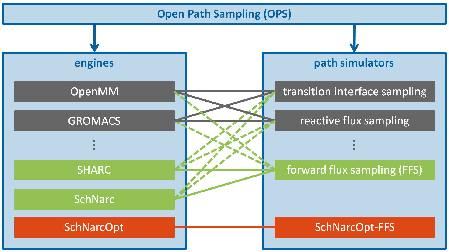
The practical implementation of NAFFS relies on two program suites. On the TSH side, we extended SHARC56, 58, 57 with a Langevin thermostat to endow the dynamics with the stochasticity required for FFS (Sec. 2.2). On the FFS side, we used Open Path Sampling (OPS),66, 67 a Python library for path sampling simulations capable to work with various MD codes. For example, OPS is interfaced with two popular MD engines: OpenMM68, 69 and GROMACS70, 71 (see gray engines in Fig. 3). We have now implemented the SHARC suite and the SchNarc72 method via the SHARC driver pySHARC73 as new general engines in OPS, see green engines in Fig. 3. Hence, any quantum chemical method compatible with the SHARC program for computing PESs and electronic properties is now also available for NAFFS simulations. SchNarc was originally developed as an interface between the SHARC program and an extension of the neural network potential SchNet74, 75 to excited-state properties.72 We do not use neural networks in this work, but because SchNarc is not based on file I/O it allows for computationally much more efficient path sampling simulations using TSH dynamics. An additional advantage of the SchNarc engine is that it opens the possibility of using neural network potentials to compute PESs in the future, further decreasing computational costs.
To accompany both engines, SHARC and SchNarc, we implemented an OPS tool to capture snapshots, i.e., individual frames of a trajectory. Such a tool is needed to describe the system at a particular point in time, where specific ranges of PESs are included in addition to the atomic positions and velocities that define the collective variables. Both, the ranges of PESs and collective variables, are used for the definition of the stable initial and final regions and as well as the definition of the FFS interfaces. We note that, as usual in OPS, we also include in our engines an additional rejection criterion for discarding trial shots if those exceed a user-given number of time steps. Although this number should be chosen such that (almost) no trajectories are discarded, such implementation is useful, as it aids, for example, the discovery of new stable minima in the region between and . From a practical point of view, a rejection criterion is also helpful to avoid very long unnecessary calculations in such a priori unknown stable minima by terminating the respective trajectory calculation and continuing with the next shot.
In OPS any engine can be combined with any TPS simulator, such as transition interface sampling42 or reactive flux sampling,76 see Fig. 3. As an additional transition path sampling method in the OPS library, here we implemented a general FFS simulator applicable to excited states, see green simulator in Fig. 3.
The advantage of both the general SHARC engines and the general FFS simulator is that they are implemented in the spirit of OPS, i.e., any engine can be combined with any path simulators, so that, in principle, now SHARC (or SchNarc) can be used with any method available in OPS (dashed green lines) and certainly both engines effectively work with FFS (solid green lines). Despite their flexibility, we have also created a dedicated SchNarcOpt engine that is combined with an optimized FFS-SchNarcOpt path simulator (red in Fig. 3), which, although specific, is computationally more efficient since it does not require file I/O. This specific NAFFS implementation has been used in the applications below in order to keep the computational cost as low as possible.
The vertical excitation and the equilibration process (recall Fig. 1) pose a necessary preliminary step prior to any NAFFS simulation. In this work, these steps are carried out in a plain SHARC/SchNarc-TSH simulation. Thus, the workflow of a NAFFS simulation begins with the flux simulation and collection of initial shooting points on the boundary of the initial region (see Fig. 2a). This process is done via the SchNarcOpt engine through OPS and it is followed by the FFS cycles (see Fig. 2b-d), executed via the SchNarcOpt-FFS path simulator in OPS.
In summary, the workflow of a typical NAFFS simulation starts with generating initial conditions (e.g., Wigner sampling and vertical excitation, see Fig. 1), and a relaxation into the initial region, followed by the NAFFS method that generates transition trajectories between the initial and final regions.
To ensure transparency and reproducibility of the obtained results, the code developed is made freely available (see Sec. S1 †).
4 Results and Discussion
As a first application of NAFFS, here we employ two dynamically relevant analytical potential energy landscapes that have been constructed to include rare events in different conditions. We deliberately choose simple analytical models for testing NAFFS rather than a real molecule because they allow for a systematic investigation of different parameters and demonstrate the broad applicability of NAFFS even in extreme situations, regardless of low or high temperature, strong or weak nonadiabaticity. Further, our models can be tuned so that NAFFS results can be compared with reference data obtained with plain brute-force TSH simulations under different conditions. These TSH calculations have been also performed via the SchNarcOpt engine through OPS. The future simulation of real molecules is straightforward, i.e., does not require any further implementation, only investing in the calculation of on-the-fly multidimensional PESs at the desired quantum chemical level of theory.
The first system features an avoided crossing between two states, see Sec. 4.1. Using this model, we demonstrate the essential functionality of NAFFS by calculating the temperature dependence of the transition rate constant with the energy barrier of the avoided crossing. Further, for this model we investigate the influence of nonadiabatic effects on the transition rate constant by varying the gap size between the PESs and thus the rareness of the event.
The second system includes a conical intersection between two states, see Sec. 4.2. This model shows richer nonadiabatic dynamics than the one-dimensional avoided crossing and allows us to focus on the dependence of the reaction rate constant on temperature and to study the contributions of trajectories with different numbers of hops.
Both models demonstrate that NAFFS yields correct results compared to reference plain brute-force TSH simulations in a fraction of the computational time and thus is ideally suited to study general rare nonadiabatic reactions.
4.1 Rare event dynamics through an avoided crossing
We define a three-dimensional potential energy landscape from two diabatic harmonic potentials of the form
| (19) |
defined in the Cartesian coordinates , , and . In -direction the potential is bi-stable with minima at separated by a barrier of height . The tight harmonic potentials acting on the and coordinates make the system effectively one-dimensional along the coordinate. In particular, the additive terms in and are invariant under a diagonalization of the diabatic Hamiltonian. However, the dynamics is coupled in all directions due to the velocity rescaling (see Eq. (15)) and decoherence scheme (see Eq. (16)). We use system-specific self-consistent units, i.e., we measure energies in units of , lengths in units of , and masses in units of , where the mass of our system is (see Sec. S2.1 † and Table S1 †) for the remainder of this Section. Time is measured in units of .
The diabatic potentials are coupled to each other by a constant coupling of , giving the diabatic Hamiltonian,
| (20) |
which upon diagonalization provides the gap between the corresponding avoiding adiabatic potentials (here labeled as ground and excited states, see Fig. 4a). This model of an avoided crossing is used to compare quantitative and qualitative results against plain brute-force TSH simulations. In this way, we demonstrate that NAFFS yields the correct reaction rate constants and evaluate its computational efficiency. Varying the temperature and the strength of the diabatic coupling gives insight into how these parameters fundamentally condition the transition rate constants.
For the first simulation we use . This is a rather strong diabatic coupling and leads to a very strongly avoided crossing, i.e. the energy gap is (see Fig. 4a), which is large compared to other choices of the coupling constant considered later. Accordingly, one expects very few nonadiabatic surface hops in the generated trajectories and a dynamics that is predominantly adiabatic in the ground state potential with occasional hops to the excited state. The ground state resembles a one-dimensional double-well potential, where we define the ground state minimum around as initial region and the ground state minimum around as final region . The two stable regions are separated by a ground state energy barrier of , see Fig. 4a.

All simulations presented in this Section employ the default TSH decoherence parameter64 (see Sec. S2.2 †) and substeps (see Eq. (10)). The remaining adjustable parameters are the temperature, the time step, and the friction constant. The time step is set to approximately , such that one oscillation in a ground state minimum consists of at least time steps, and, hence, the dynamics of the system can be adequately captured. The temperature is set to , such that the ground state barrier height is . This barrier height is sufficiently large to make the barrier crossing a rare event possible and, at the same time, sufficiently low to enable the observation of transition events in brute-force TSH simulations.
The rate constant of a transitions from to depends on the friction constant that appears in the Langevin equation (see Eq. (17)).77 In particular, the rate constant shows a maximum as a function of the friction constant, known as the Kramers turnover.77, 78 For smaller and larger values of the rate constant decreases: at low friction because of slow energy exchange of the system with the environment and at high friction due to slow diffusion at the barrier top. The maximum transition rate constant is expected to occur for a friction constant at which the energy dissipated as the system crosses the barrier is about . For a barrier shaped like an inverted parabola, this conditions implies , where is the friction constant at which the turnover occurs and is the frequency of the unstable mode at the barrier top. For the parameters selected here, the turnover friction is . Hence, the friction coefficient selected for our simulations, , is slightly higher than the turnover friction.
For the brute-force TSH trajectory, we run million time steps, and for the analysis, we define the ground state region as the initial region , and the ground state region as the final region . A representative cutout of the TSH trajectory can be seen in Fig. 4b. It shows the typical behavior of a rare event, i.e., it oscillates for a long time in one of the two regions or before it undergoes a fast transition to the other region, where it oscillates again. As the diabatic coupling is very large, the crossing is strongly avoided and we expect small nonadiabatic effects. Indeed, the system spends only very short periods of time in the excited state, see orange circles in Fig. 4b. The corresponding reaction rate constant for the transition from the initial region to the final region obtained with the brute-force TSH is , see Table 1. This result nicely agrees with that obtained by the NAFFS simulation , which aside marginal statistical deviations, demonstrates the quantitative accuracy of our implementation. The computational details for the NAFFS simulation are given in Table S2 †.
| TSH | NAFFS | |
|---|---|---|
| rate constant () | ||
| number of transition paths | ||
| mean transition time | ||
| std transition time | ||
| mean number of hops | ||
| std number of hops |
Figures 4c and 4d show the superimposed transition paths connecting the regions and , as obtained from TSH and NAFFS simulations. The mean time that a transition path takes to go from to and the average number of hops occurring during the transition paths are also collected in Table 1, together with their corresponding standard deviations. The larger standard deviation for the transition time in TSH compared to NAFFS stems from the overall lower number of transition paths obtained with TSH and some outlying long transition paths among them. The good qualitative and quantitative agreement between NAFFS and TSH values confirms that the NAFFS simulation correctly samples transition paths.
In order to demonstrate the applicability of NAFFS in harsher conditions, we now decrease the temperature, which effectively increases the barrier and thus the rareness of the event. To avoid variations of the rate constant at different temperatures due to the definition of the boundaries of the stable regions and , we fix as and as on the ground state for the remaining simulations on this model. We expect the temperature dependence of calculated rate constants to follow Arrhenius’ law,
| (21) |
with prefactor . The reaction rate constants obtained with NAFFS, shown in Figure 5a as a function of the inverse temperature, fit Arrhenius’ law remarkably well.

Table 2 illustrates the computational efficiency of NAFFS against TSH, showing that the speedup of NAFFS versus TSH increases with the rareness of the transition.
Note that the average number of time steps needed to obtain one NAFFS trajectory depends on the acceptance probabilities for the various interfaces (especially of the last shooting interface where the total number of final transition paths is determined), and, hence, on the choice of the interface placements. This explains that the average number of time steps required to obtain one reactive NAFFS path is always of the same order of magnitude, in stark contrast to the TSH simulations, which require an increasingly larger number of steps with decreasing temperature. Accordingly, for the lowest temperature (largest barrier height ), NAFFS sampled transition paths in about one million time steps (flux calculation included) whereas TSH sampled only in the same amount of time steps. This implies a speed up of almost in favor of NAFFS, i.e., a sampling acceleration of two orders of magnitude. We note that at this low temperature, an accurate rate constant calculation is no longer possible within reason with brute-force TSH, but well feasible with NAFFS.
| TSH (time steps) | NAFFS (time steps) | speedup factor | |
|---|---|---|---|
Finally, since the dynamics with is predominantly adiabatic in the ground state potential, we investigate the effect of varying the diabatic coupling from to , thus decreasing the diabatic gap from to , and thus increasing the nonadiabaticity of the avoided crossing. The barrier height in terms of is kept constant and equal to for all simulations. The rate constant is expected to decrease with smaller gaps, as the nonadiabatic effects increase, i.e., the number of hops in the adiabatic representation increases, and, thus, the probability of a transition for a trajectory that reaches the energy barrier is lower than for systems with higher gap sizes. In other words, with smaller gaps, the nonadiabatic effects become more an obstacle that the system must overcome to complete a transition in addition to the potential energy barrier. In the limit of no diabatic coupling ( and, hence, ), the system is diabatically trapped, i.e., the dynamics purely evolves on one diabatic state, and the transition rate constant is zero.
As expected, the calculated reaction rate constants are lower for smaller gap sizes, see Figure 5b. The probability that a trajectory coming from the initial region hops to the excited state in the vicinity of the barrier, oscillates there for one period and then falls back to the ground state in direction of due to the inertia, increases with decreasing gap size, i.e., the closer the adiabatic states come to each other. Accordingly, the mean number of surface hops in transition paths also increases with decreasing gap size, see Fig. 5c. We fitted the obtained rate constants (see Fig. 5b) according to the Landau-Zener-type formula79, 80, 81
| (22) |
where is the ground state transition rate constant, and is a fitting parameter . This expression approximately describes the dependence of the reaction rate constant on the gap size.77 As shown in Fig. 5b, the fit nicely reproduces our data. Even for small energy gap sizes, and, thus, highly nonadiabatic situations, the NAFFS and TSH simulation rate constants agree (see Fig. S1 †), further validating our method.
4.2 Rare event dynamics through a conical intersection
To examine the application of NAFFS to rare event dynamics in the vicinity of an explicit conical intersection, we consider a model with two coupled diabatic potential energy surfaces,
| (23) |
and
| (24) |
with Cartesian coordinates , , and and parameters , , , , . The narrow harmonic potential around the coordinate allows us to consider the potential energy landscape as a function of two variables, and . Again, all values are given in system-specific self-consistent units (see Sec. S2.1 † and Table S1 †) and the mass is . The coupling between the two diabatic PESs is given by
| (25) |
with the prefactor , and , resulting in the adiabatic PESs shown in Fig. 6a-b.

We choose the default decoherence parameter 64 (see Sec. S2.3 †) and substeps (see Eq. (10)). As meaningful parameter values for the propagation using the Langevin thermostat, we choose a time step of , a temperature , and a friction coefficient . In contrast to the model discussed in Sec. 4.1, here the rare event is not due to a high barrier, as this is only , but due to a small diabatic coupling that makes the system stay preferably on one diabatic surface (i.e., diabatic trapping). Accordingly, the dynamics shows frequent hops between the ground and excited adiabatic PESs in regions close to the conical intersection (see Fig. 6c), i.e., in general twice during a typical oscillation period in one of the minima. Hence, in this case the rare event is a rare hop in the diabatic representation, i.e., a transition between the two diabatic PESs and (Eq. (23)-(24)). The initial region and final region are defined by and , respectively, plus the additional condition that the system needs to be located in the ground state. The stable region’s boundaries also correspond to the first and last interface in the NAFFS simulation.
For this model, we performed a plain brute-force TSH simulation of million time steps. The resulting rate constant, , for the transition from to agrees very well with the rate constant obtained using a NAFFS calculation, (, performed with million time steps in the flux simulation followed by shots per interface (see Table 3). Computational details for the NAFFS simulations are given in Table S3 of Sec. S2.2 †. A second NAFFS simulation of half the size of the previous one ( million time steps and shots per interface, see Sec. S2.3 †) still yields the correct result, namely , highlighting the efficiency of NAFFS.
| TSH | NAFFS | |
|---|---|---|
| rate constant () | ||
| number of transition paths | ||
| mean transition time | ||
| std transition time | ||
| mean number of hops | ||
| std number of hops |
The transition paths obtained by the NAFFS simulations (Fig. 6d) are very similar to the ones obtained from brute-force TSH simulations (Fig. S2a †), demonstrating that NAFFS correctly samples transition paths in strong nonadiabatic regimes. Therefore, we next change the parameters of our model system to study it under different conditions. First, we investigate the dependence of the reaction rate constant on temperature. As can be seen in Fig. 7a, due to the stronger nonadiabaticity of the system, the dependence is stronger than in the case of the avoided crossing (recall Fig. 5a), i.e., the slope in a vs. plot is steeper than that given by Arrhenius’ law (Eq. (21)) with an activation energy that equals the ground state barrier height (see Fig. 7a). Fitting the reaction rate constants with the expression
| (26) |
with constant yields an effective activation energy of , which is significantly higher than the ground state energy barrier of . This means that the nonadiabatic effects lead to an additional barrier that decreases the probability of the system to undergo a transition.
The obtained NAFFS transition paths show the expected qualitative behavior for different temperatures: their distribution is broader for higher temperatures as the system has more energy available, and is narrower for low temperatures where the transition paths are located in the region around the conical intersection. In regions close to the conical intersection, the energy that the system needs to transition to the final region is lower than in regions far away from the conical intersection, see the narrower distribution of transition paths in Fig. 6e along the diagonal direction compared to Fig. 6d. At low temperatures (see Fig. 6e), the rare event is mainly determined by the high potential barrier, whereas for high temperatures (see Fig. 6d), the rareness is predominantly caused by the nonadiabatic effects.

Figure 7b shows that the rate constants of reactive paths that exhibit a given number of hops between the ground and the excited adiabatic PESs differ from each other. In general, the fraction of transition paths that do not undergo hops increases with decreasing temperature, while the fraction of transition paths that feature hops decreases with decreasing temperature (see Fig. S2b †). This is because the system needs energy to undergo hops to the excited state, but has less energy available the lower the temperature is (see Fig. S2d †). Note that due to using velocity rescaling (see Eq. (15), the number of hops to the excited state might be slightly overestimated, because the system can use all the kinetic energy along the velocity vector to perform a hop. Rescaling along the NAC direction—usually regarded as more accurate82—would lead to fewer upwards hops, because less kinetic energy is usually available along the NAC direction. For simplicity, here we use velocity rescaling.
Since we defined the initial and final regions and in the adiabatic ground state, a transition path from to can only have an even number of hops in the adiabatic representation. The “hop-dependent” rate constants (see Fig. 7b) are fitted according to Eq. (26), yielding effective activation energies for transition paths with a certain number of hops between the ground and excited adiabatic PESs. increases with increasing number of hops, which again agrees with the necessity to spend energy for hopping events (see Fig. 7c). The effective activation energy for transition paths showing zero hops, i.e., reaction paths evolving entirely in the ground state, is , which within the range of uncertainty aligns accurately with the ground state energy barrier of . Hence, transition paths evolving only in the ground state follow Arrhenius’ law even if this ground state is part of a highly nonadiabatic PES landscape. Furthermore, nonadiabatic transition paths also follow approximately Arrhenius’ law, but with a higher effective activation energy. The latter can be understood when thinking about nonadiabatic effects as prolonging the transition path (e.g., because of turning around and having to come back again), which can be compensated by higher energies and hence the reaction barrier seems effectively higher.
An estimate of the computational savings obtained when using our NAFFS implementation is shown in Table 4. As in the case of the rare event dynamics through an avoided crossing (Table 2), here we also achieve a speedup factor of about for the largest barrier height considered.
| TSH (time steps) | NAFFS (time steps) | speedup factor | |
|---|---|---|---|
5 Conclusions
In this work, we have introduced a nonadiabatic forward flux sampling (NAFFS) method that uses the trajectory surface hopping (TSH) algorithm for the underlying dynamics simulation. This method extends the previous fields of application of FFS to capture rare events in electronically excited systems, such as those initiated by the absorption of a photon. NAFFS is therefore suitable to deal with excited-state processes that occur on very long time scales, which cannot be otherwise accessed with plain brute-force TSH simulations. Using two models that exemplify different regimes of rareness and nonadiabaticity, we demonstrate that NAFFS produces quantitatively and qualitatively correct results at a computational cost that is two orders of magnitude lower than that of conventional TSH molecular dynamics simulations. Unlike previous efforts to develop nonadiabatic transition path sampling methods,38 our method does not need to propagate trajectories back in time, and, hence, avoids serious problems in long simulations that include several hopping events.40, 37
The presented approach is particularly promising to investigate photoinduced chemical reactions that are hindered by potential energy barriers or very small nonadiabatic couplings, and thus take a long time to occur. Exciting examples include DNA damage and repair processes,83, 84 enone [2+2] photocycloadditions85 and many more.
Conflicts of interest
There are no conflicts to declare.
Acknowledgements
The authors thank the University of Vienna for continuous support, in particular the one provided in the framework of the research platform ViRAPID. M. X. T., and L. G. appreciate additional support provided by the Austrian Science Fund, W 1232 (MolTag). The computational results presented have been achieved (in part) using the Vienna Scientific Cluster (VSC). The authors thank the SHARC development team, and the ViRAPID members for insightful discussions. We thank Barbara Wagner for her contributions to some NAFFS calculations.
References
- Honda et al. 2012 K. Honda, M. Konishi, M. Kawai, A. Yamada, Y. Takahashi, Y. Hoshino and S. Inoue, Nat. Prod. Commun., 2012, 7, 459–462.
- Candish et al. 2022 L. Candish, K. D. Collins, G. C. Cook, J. J. Douglas, A. Gómez-Suárez, A. Jolit and S. Keess, Chem. Rev., 2022, 122, 2907–2980.
- Feliu et al. 2018 N. Feliu, E. Neher and W. J. Parak, Science, 2018, 359, 633–635.
- Holland et al. 2020 J. P. Holland, M. Gut, S. Klingler, R. Fay and A. Guillou, Chem. Eur. J., 2020, 26, 33–48.
- Tian et al. 2018 Molecular devices for solar energy conversion and storage, ed. H. Tian, G. Boschloo and A. Hagfeldt, Springer, Singapore, 2018.
- Ciamician 1912 G. Ciamician, Science, 1912, 36, 385–394.
- De Nalda and Bañares 2013 Ultrafast Phenomena in Molecular Sciences : Femtosecond Physics and Chemistry, ed. R. De Nalda and L. Bañares, Springer International Publishing AG, Cham, 2013.
- Domcke et al. 2011 Conical intersections: theory, computation and experiment, ed. W. Domcke, D. R. Yarkony and H. Köppel, World Scientific, 2011.
- Turro 1965 N. J. Turro, Molecular Photochemistry, 1965, p. 148.
- Zwicker et al. 1963 E. F. Zwicker, L. I. Grossweiner and N. C. Yang, J. Am. Chem. Soc., 1963, 85, 2671–2672.
- Hammes-Schiffer and Tully 1995 S. Hammes-Schiffer and J. C. Tully, J. Chem. Phys., 1995, 103, 8513–8527.
- Dellago and Bolhuis 2009 C. Dellago and P. G. Bolhuis, Advanced Computer Simulation Approaches for Soft Matter Sciences III. Adv. Polym. Sci., Springer, Berlin, Heidelberg, 2009, pp. 167–233.
- Lindh and González 2020 Quantum Chemistry and Dynamics of Excited States: Methods and Applications, ed. R. Lindh and L. González, John Wiley & Sons, 2020.
- Curchod and Martínez 2018 B. F. Curchod and T. J. Martínez, Chem. Rev., 2018, 118, 3305–3336.
- Reiter et al. 2020 S. Reiter, D. Keefer and R. De Vivie-Riedle, Quantum Chemistry and Dynamics of Excited States: Methods and Applications, Wiley & Sons, 2020, ch. 11, pp. 355–381.
- Crespo-Otero and Barbatti 2018 R. Crespo-Otero and M. Barbatti, Chem. Rev., 2018, 118, 7026–7068.
- Mai et al. 2020 S. Mai, P. Marquetand and L. González, Quantum Chemistry and Dynamics of Excited States: Methods and Applications, John Wiley & Sons, 2020, ch. 16, pp. 499–530.
- Zobel et al. 2021 J. P. Zobel, T. Knoll and L. González, Chem. Sci., 2021, 12, 10791–10801.
- Westermayr et al. 2019 J. Westermayr, M. Gastegger, M. F. Menger, S. Mai, L. González and P. Marquetand, Chem. Sci., 2019, 10, 8100–8107.
- Li et al. 2021 J. Li, P. Reiser, B. R. Boswell, A. Eberhard, N. Z. Burns, P. Friederich and S. A. Lopez, Chem. Sci., 2021, 12, 5302–5314.
- Westermayr and Marquetand 2020 J. Westermayr and P. Marquetand, Mach. Learn.: Sci. Technol., 2020, 1, 043001.
- Westermayr and Marquetand 2021 J. Westermayr and P. Marquetand, Chem. Rev., 2021, 121, 9873–9926.
- Torrie and Valleau 1977 G. Torrie and J. Valleau, Journal of Computational Physics, 1977, 23, 187–199.
- Ciccotti and Ferrario 2004 G. Ciccotti and M. Ferrario, Molecular Simulation, 2004, 30, 787–793.
- Grubmüller et al. 1996 H. Grubmüller, B. Heymann and P. Tavan, Science, 1996, 271, 997–999.
- Voter 1997 A. F. Voter, Phys. Rev. Lett., 1997, 78, 3908–3911.
- Faradjian and Elber 2004 A. K. Faradjian and R. Elber, The Journal of Chemical Physics, 2004, 120, 10880–10889.
- Laio and Parrinello 2002 A. Laio and M. Parrinello, Proceedings of the National Academy of Sciences, 2002, 99, 12562–12566.
- E et al. 2002 W. E, W. Ren and E. Vanden-Eijnden, Phys. Rev. B, 2002, 66, 052301.
- Dellago et al. 1998 C. Dellago, P. G. Bolhuis, F. S. Csajka and D. Chandler, J. Chem. Phys., 1998, 108, 1964–1977.
- Allen et al. 2005 R. J. Allen, P. B. Warren and P. R. Ten Wolde, Phys. Rev. Lett., 2005, 94, 018104.
- Allen et al. 2006 R. J. Allen, D. Frenkel and P. R. Ten Wolde, J. Chem. Phys., 2006, 124, 024102.
- Allen et al. 2006 R. J. Allen, D. Frenkel and P. R. Ten Wolde, J. Chem. Phys., 2006, 124, 194111.
- Pieri et al. 2021 E. Pieri, D. Lahana, A. M. Chang, C. R. Aldaz, K. C. Thompson and T. J. Martínez, Chem. Sci., 2021, 12, 7294–7307.
- Aldaz et al. 2018 C. Aldaz, J. A. Kammeraad and P. M. Zimmerman, Phys. Chem. Chem. Phys., 2018, 20, 27394–27405.
- Lindner et al. 2019 J. O. Lindner, K. Sultangaleeva, M. I. Röhr and R. Mitrić, J. Chem. Theory Comput., 2019, 15, 3450–3460.
- Schile and Limmer 2018 A. J. Schile and D. T. Limmer, J. Chem. Phys., 2018, 149, 214109.
- Sherman and Corcelli 2016 M. C. Sherman and S. A. Corcelli, J. Chem. Phys., 2016, 145, 034110.
- Tully 1990 J. C. Tully, J. Chem. Phys., 1990, 92, 1061–1071.
- Subotnik and Rhee 2015 J. E. Subotnik and Y. M. Rhee, J. Phys. Chem. A, 2015, 119, 990–995.
- Hammes-Schiffer and Tully 1995 S. Hammes-Schiffer and J. C. Tully, The Journal of Chemical Physics, 1995, 103, 8528–8537.
- Van Erp et al. 2003 T. S. Van Erp, D. Moroni and P. G. Bolhuis, J. Chem. Phys., 2003, 118, 7762–7774.
- Allen et al. 2009 R. J. Allen, C. Valeriani and P. R. Ten Wolde, J. Phys.: Condens. Matter, 2009, 21, 1–40.
- Bolhuis and Swenson 2021 P. G. Bolhuis and D. W. Swenson, Adv. Theor. Simul., 2021, 4, 1–14.
- Peters 2016 B. Peters, Annu. Rev. Phys. Chem., 2016, 67, 669–690.
- Escobedo et al. 2009 F. A. Escobedo, E. E. Borrero and J. C. Araque, J. Phys.: Condens. Matter, 2009, 21, 333101.
- Berkov et al. 2021 D. Berkov, E. K. Semenova and N. L. Gorn, Phys. Rev. Lett., 2021, 127, 247201.
- Borrero et al. 2011 E. E. Borrero, M. Weinwurm and C. Dellago, J. Chem. Phys., 2011, 134, 244118.
- Hussain and Haji-Akbari 2020 S. Hussain and A. Haji-Akbari, J. Chem. Phys., 2020, 152, 060901.
- Bolhuis and Dellago 2015 P. G. Bolhuis and C. Dellago, Eur. Phys. J. Spec. Top., 2015, 224, 2409–2427.
- Dellago et al. 2006 C. Dellago, P. G. Bolhuis and P. L. Geissler, Lect. Notes Phys., 2006, 703, 349–391.
- Borrero and Escobedo 2008 E. E. Borrero and F. A. Escobedo, J. Chem. Phys., 2008, 129, 024115.
- Verlet 1967 L. Verlet, Phys. Rev., 1967, 159, 98–103.
- Verlet 1968 L. Verlet, Phys. Rev., 1968, 165, 201–214.
- Grønbech-Jensen et al. 2014 N. Grønbech-Jensen, N. R. Hayre and O. Farago, Comput. Phys. Commun., 2014, 185, 524–527.
- Richter et al. 2011 M. Richter, P. Marquetand, J. González-Vázquez, I. Sola and L. González, J. Chem. Theory Comput., 2011, 7, 1253–1258.
- Mai et al. 2015 S. Mai, P. Marquetand and L. González, Int. J. Quantum Chem., 2015, 115, 1215–1231.
- Mai et al. 2018 S. Mai, P. Marquetand and L. González, Wiley Interdiscip. Rev.: Comput. Mol. Sci., 2018, 8, 1–23.
- Tully and Preston 1971 J. C. Tully and R. K. Preston, J. Chem. Phys., 1971, 55, 562–572.
- Nelson et al. 2020 T. R. Nelson, A. J. White, J. A. Bjorgaard, A. E. Sifain, Y. Zhang, B. Nebgen, S. Fernandez-Alberti, D. Mozyrsky, A. E. Roitberg and S. Tretiak, Chem. Rev., 2020, 120, 2215–2287.
- Fabiano et al. 2008 E. Fabiano, T. W. Keal and W. Thiel, Chem. Phys., 2008, 349, 334–347.
- Plasser et al. 2019 F. Plasser, S. Mai, M. Fumanal, E. Gindensperger, C. Daniel and L. González, J. Chem. Theory Comput., 2019, 15, 5031–5045.
- Heindl and González 2021 M. Heindl and L. González, J. Chem. Phys., 2021, 154, 144102.
- Granucci et al. 2010 G. Granucci, M. Persico and A. Zoccante, J. Chem. Phys., 2010, 133, 134111.
- Grønbech-Jensen and Farago 2013 N. Grønbech-Jensen and O. Farago, Mol. Phys., 2013, 111, 983–991.
- Swenson et al. 2019 D. W. Swenson, J. H. Prinz, F. Noe, J. D. Chodera and P. G. Bolhuis, J. Chem. Theory Comput., 2019, 15, 813–836.
- Swenson et al. 2019 D. W. Swenson, J. H. Prinz, F. Noe, J. D. Chodera and P. G. Bolhuis, J. Chem. Theory Comput., 2019, 15, 837–856.
- Eastman and Pande 2010 P. Eastman and V. S. Pande, Comput. Sci. Eng., 2010, 12, 34–39.
- Eastman et al. 2013 P. Eastman, M. S. Friedrichs, J. D. Chodera, R. J. Radmer, C. M. Bruns, J. P. Ku, K. A. Beauchamp, T. J. Lane, L. P. Wang, D. Shukla, T. Tye, M. Houston, T. Stich, C. Klein, M. R. Shirts and V. S. Pande, J. Chem. Theory Comput., 2013, 9, 461–469.
- Van Der Spoel et al. 2005 D. Van Der Spoel, E. Lindahl, B. Hess, G. Groenhof, A. E. Mark and H. J. Berendsen, J. Comput. Chem., 2005, 26, 1701–1718.
- Hess et al. 2008 B. Hess, C. Kutzner, D. Van Der Spoel and E. Lindahl, J. Chem. Theory Comput., 2008, 4, 435–447.
- Westermayr et al. 2020 J. Westermayr, M. Gastegger and P. Marquetand, J. Phys. Chem. Lett., 2020, 11, 3828–3834.
- Plasser et al. 2019 F. Plasser, S. Gómez, M. F. Menger, S. Mai and L. González, Phys. Chem. Chem. Phys., 2019, 21, 57–69.
- Schütt et al. 2017 K. T. Schütt, P. J. Kindermans, H. E. Sauceda, S. Chmiela, A. Tkatchenko and K. R. Müller, Adv. Neural Inf. Process. Syst., 2017, 30, 992–1002.
- Schütt et al. 2018 K. T. Schütt, H. E. Sauceda, P. J. Kindermans, A. Tkatchenko and K. R. Müller, J. Chem. Phys., 2018, 148, 241722.
- van Erp and Bolhuis 2005 T. S. van Erp and P. G. Bolhuis, J. Comput. Phys., 2005, 205, 157–181.
- Hänggi et al. 1990 P. Hänggi, P. Talkner and M. Borkovec, Rev. Mod. Phys., 1990, 62, 251–341.
- Rondin et al. 2017 L. Rondin, J. Gieseler, F. Ricci, R. Quidant, C. Dellago and L. Novotny, Nature Nanotechnology, 2017, 12, 1130–1133.
- Novaro et al. 2012 O. Novaro, M. D. A. Pacheco-Blas and J. H. Pacheco-Sánchez, Adv. Phys. Chem., 2012, 2012, 720197.
- Zener 1932 C. Zener, Proc. R. Soc. London, Ser. A, 1932, 137, 696–702.
- Landau 1932 L. D. Landau, Phys. Z. Sowjetunion, 1932, 2, 118.
- Subotnik et al. 2016 J. E. Subotnik, A. Jain, B. Landry, A. Petit, W. Ouyang and N. Bellonzi, Annu. Rev. Phys. Chem., 2016, 67, 387–417.
- Barbatti et al. 2015 M. Barbatti, A. Borin and S. Ullrich, Photoinduced Phenomena in Nucleic Acids I and II, Springer, Cham, Topics in Current Chemistry edn, 2015, vol. 355 and 356.
- Improta et al. 2016 R. Improta, F. Santoro and L. Blancafort, Chem. Rev., 2016, 116, 3540–3593.
- Brimioulle and Bach 2013 R. Brimioulle and T. Bach, Science, 2013, 342, 840–843.