Topological susceptibility of or non-linear -model: is it divergent or not?
Abstract
The topological susceptibility of models is expected, based on perturbative computations, to develop a divergence in the limit , where these models reduce to the well-known non-linear -model. The divergence is due to the dominance of instantons of arbitrarily small size and its detection by numerical lattice simulations is notoriously difficult, because it is logarithmic in the lattice spacing. We approach the problem from a different perspective, studying the behavior of the model when the volume is fixed in dimensionless lattice units, where perturbative predictions are turned into more easily checkable behaviors. After testing this strategy for and , we apply it to , adopting at the same time a multicanonic algorithm to overcome the problem of rare topological fluctuations on asymptotically small lattices. Our final results fully confirm, by means of purely non-perturbative methods, the divergence of the topological susceptibility of the model.
pacs
12.38.Aw, 11.15.Ha, 12.38.Gc, 12.38.Mh1 Introduction
The models are quantum field theories that play an important role in the study of the non-perturbative properties of gauge theories, as they share many intriguing features with Yang–Mills theories, such as confinement, the existence of a non-trivial topological structure and the related dependence on the topological parameter . D’Adda et al. 1978; Shifman 2012; Vicari and Panagopoulos 2009. These theories are amenable to be treated exactly by analytic means in certain regimes, but have also been extensively explored by means of Monte Carlo (MC) simulations on the lattice, since they constitute the perfect theoretical laboratory to test new numerical methods in view of an application to the more complicated physical gauge theories.
At large-, models admit a expansion which is similar to the ’t Hooft large- expansion of QCD. These models, however, admit an analytic solution in this regime, and the large- limit of the vacuum energy is well known both analytically and numerically Witten 1980; Witten 1998; Rossi and Vicari 1993; Rossi 2016; Campostrini and Rossi 1991; Campostrini et al. 1992a; Campostrini et al. 1992b; Campostrini and Rossi 1993; Bonati et al. 2016; Bonanno et al. 2019; Berni et al. 2019. An important difference between models and Yang–Mills theories emerges in the opposite, small- limit. Indeed, in the limit, where the theory becomes equivalent to the non-linear -model (which has been widely studied both analytically and numerically in the literature Forster 1977; Berg and Lüscher 1981; Haldane 1983a; Haldane 1983b; Bhanot and David 1985; Haldane 1985; Wiegmann 1985; Affleck and Haldane 1987; Hasenfratz et al. 1990; D’Elia et al. 1995; D’Elia et al. 1997; Blatter et al. 1996; Burkhalter et al. 2001; Controzzi and Mussardo 2004; Alles and Papa 2008; Nogradi 2012; Azcoiti et al. 2012; Alles et al. 2014; Bietenholz et al. 2018; Bruckmann et al. 2019; Sulejmanpasic and Tanizaki 2018; Sulejmanpasic et al. 2020; Thomas and Monahan 2022; Marino et al. 2022), a pathological behavior emerges, which has no analogue in the Yang–Mills case, where instead the approach from small to large is much smoother Bonati et al. 2016; Bonanno et al. 2021; Kitano et al. 2021a; Kitano et al. 2021b.
The semi-classical picture predicts a divergence of the topological susceptibility for , which survives the renormalization procedure. Various studies have already tried to check this prediction by lattice numerical simulations, and while there is a general consensus that the prediction is verified, the issue is not completely settled. For example, while various works about the non-linear -model found numerical evidence supporting that is divergent in the continuum limit (see, e.g., Refs. Bietenholz et al. 2018; Thomas and Monahan 2022), a recent investigation Berni et al. 2020 from some of the authors of the present paper, considering both direct simulations at and the limit of models, pointed out some difficulties in making a definite statement.
The main difficulty can be related to the fact that the divergence is of ultraviolet (UV) origin, i.e., it is related to the presence of semiclassical solutions with non-zero topological charge (instantons) at arbitrarily small scales. As a consequence, lattice studies need to check the emergence of a divergent behavior as the lattice spacing : this task can be ambiguous, since the behavior could be barely distinguishable from a badly convergent behavior in a wide range of lattice spacings. For instance, even for the finiteness of could be definitely established only recently (see, e.g., Ref. Berni et al. 2020, where two different strategies led consistent results).
The purpose of the present study is to develop a novel strategy, in order to make the problem better defined and reach more definite conclusions. In practice, we will approach the continuum limit keeping the ratio between the UV and the infrared (IR) cutoffs fixed, i.e., working at fixed volume in lattice units, and then considering the same procedure for different values of the dimensionless volume, a strategy which resembles some aspects of the determination of the step scaling beta-function on the lattice (see, e.g., Ref. Del Debbio and Ramos 2021 for a recent review on the topic). As we will discuss in more details in the following, within this framework the original divergent behavior of the topological susceptibility is turned into a convergent (as opposed to vanishing) continuum limit, which is much easier to check numerically, as indeed we will manage to do.
A drawback of this strategy is that one is forced to study volumes of arbitrarily small size in physical units, where topological fluctuations are extremely rare and a precise determination of the topological susceptibility could require an unfeasible statistics. This problem is easily solved by adopting a multicanonical algorithm Berg and Neuhaus 1991, which has been recently employed to face the same issue in Refs. Jahn et al. 2018; Bonati and D’Elia 2018; Bonati et al. 2018; Athenodorou et al. 2022. The general idea is to add a bias potential to the action, so that the probability of visiting suppressed topological sectors is enhanced; the MC averages with respect to the original distribution are then obtained by means of an exact standard reweighting procedure.
This paper is organized as follows. In Sec. 2 we give a brief review about models and their topological properties. In Sec. 3 we describe our numerical setup and our strategy to compute the continuum limit of on asymptotically small lattices, including a description of the adopted multicanonical algorithm. In Sec. 4 we present and discuss our numerical results, including also an application of the same method to and , in order to check consistency with previous results in the literature for these models Petcher and Lüscher 1983; Campostrini et al. 1992b; Lian and Thacker 2007; Berni et al. 2020. Finally, in Sec. 5, we draw our conclusions.
2 Continum theory
The Euclidean action of models can be written in terms of a matter field , a complex -component scalar field satisfying , and of an auxiliary non propagating gauge field . In the presence of the topological term, the action reads
| (1) |
where is the ’t Hooft coupling, is the covariant derivative and
| (2) |
is the integer-valued topological charge.
The -dependent vacuum energy density, using the path-integral formulation of the theory, is given by
| (3) |
where is the space-time volume. Assuming that is an analytic function of around , one can Taylor expand it around this point; at leading order, one has Vicari and Panagopoulos 2009; Bonati et al. 2016:
| (4) |
where is the topological susceptibility
| (5) |
To better understand the origin of the divergence of in the limit, it is useful to recall that, in the semi-classical approximation, the path-integral is evaluated by integrating fluctuations around instanton solutions, and it is reduced to an ordinary integral of the instanton density. At leading order, the instanton density of models is given, as a function of the instanton size, by Lüscher 1982:
| (6) |
For , , i.e., it develops an UV divergence for . This means that the divergence of in this case can be traced back to the proliferation of small-size instantons with vanishing size , whose density grows proportionally to .
3 Numerical methods
In this section we discuss various aspects related to the discretization of the models and of the observables, in particular those related to topology, and to the employed numerical strategies.
3.1 Discretization details
We discretized space-time through a square lattice with sites and periodic boundary conditions, and the continuum action (1) through the tree-level Symanzik-improved lattice action Campostrini et al. 1992a:
| (7) |
where and are improvement coefficients, is the inverse bare coupling, are the matter fields, satisfying , and are gauge link variables. Symanzik improvement cancels out logarithmic corrections to the leading continuum scaling Symanzik 1983, improving convergence towards the continuum limit.
In this limit, approached taking , a vanishing lattice spacing can be traded for a divergent lattice correlation length . In order to fix , in this work we chose the second moment correlation length , defined in the continuum theory as
| (8) |
where denotes the two-point connected correlation function of the projector :
| (9) |
A lattice discretization of Eq. (8) can be obtained from the Fourier transform of , which is the lattice counterpart of Eq. (9) Caracciolo and Pelissetto 1998:
| (10) |
3.2 Topology on the lattice and smoothing
There are several possible discretizations of the topological charge (2), all yielding the same continuum limit for the topological susceptibility and other quantities relevant to -dependence, when discretization effects are properly taken care of. Generally speaking, lattice definitions are related to the continuum one by Campostrini et al. 1988; Farchioni and Papa 1993:
| (11) |
where is a finite multiplicative renormalization factor. For this reason, lattice discretizations of are in general not integer-valued. The most simple discretization can be defined in terms of the plaquette as:
| (12) |
However, it is possible to work out geometric discretizations of the topological charge Berg and Lüscher 1981; Campostrini et al. 1992a, which always result in integer values for every configuration, i.e., definitions with . In particular, we adopted the geometric definition that can be built from the link variables Campostrini et al. 1992a:
| (13) |
Although has , renormalization effects are still present when computing because of dislocations Berg 1981; Campostrini et al. 1992b. Dislocations are UV fluctuations of the background gauge field that make establishing the winding number of the configuration ambiguous. The net effect is that dislocations result in an additive renormalization when computing the lattice topological susceptibility Alles et al. 1998; D’Elia 2003. Such renormalization diverges in the continuum limit and thus must be removed.
Being dislocations the result of UV fluctuations at the scale of the lattice spacing, computing the geometric charge on smoothed configurations is sufficient to remove their unphysical contribution, while preserving the background topological structure of the gauge fields. Indeed, smoothing brings a configuration closer to a local minimum of the action, thus dumping UV fluctuations while, at the same time, preserving the physical topological signal.
Many different smoothing algorithms have been proposed in the literature, such as stout smearing, gradient flow, or cooling, all giving consistent results when properly matched with each other (see Refs. Bonati and D’Elia 2014; Alexandrou et al. 2015 for more details). For this reason, we chose cooling for its numerical cheapness. This method consists in a sequence of steps in which the configuration approaches a local minimum of the action by iteratively aligning both link variables and site variables to their relative local force. Since the choice of the action that is locally minimized during cooling is irrelevant Alexandrou et al. 2015, we adopted the unimproved one for this purpose, meaning that the local forces along which the and fields are aligned are computed from the action in Eq. (7) with and . In the end, thus, we define:
| (14) |
It is worth mentioning that smoothing methods act as diffusive processes, thus modifying the UV behavior of the fields below a smoothing radius which is proportional to the square root of the amount of smoothing performed (e.g., to in our case). When is finite, the choice of is not critical because the physical topological signal is well separated from the length scale introduced by the smoothing procedure. As a consequence, in such cases exhibits a plateau upon increasing above a certain threshold, and no residual dependence on is observed on continuum-extrapolated results.
The pathological case of the model is, instead, different in this respect, since we exactly aim at probing the sensitivity of to the contribution of small instantons, which are however smoothed away below (see Ref. Bietenholz et al. 2018, where the dependence of the topological susceptibility of the non-linear model on the gradient flow time is discussed). In particular, in our setup where is kept fixed as , the quantity is a relevant parameter and we expect the continuum limit of to depend on its value. Thus, we will extrapolate our results towards in order to ensure that no relevant contribution coming from small length scales is lost.
Concerning updating algorithms, models at small do not require any particular strategy to decorrelate the topological charge Berni et al. 2020, contrary to the large- case, which is plagued by a severe topological critical slowing down Del Debbio et al. 2004; Lüscher and Schaefer 2011; Hasenbusch 2017; Bonanno et al. 2019; Berni et al. 2019; Bonanno et al. 2021; Bonanno et al. 2022. As a matter of fact, models at small are dominated by small instantons, which are more easily decorrelated by means of local field updates. Thus, we will adopt local updating algorithms such as the Over-Relaxation (OR) and the over-Heat-Bath (HB) Campostrini et al. 1992a. An issue is however represented by the dominance of the sector on small physical volumes, which is discussed in more details in Sec. 3.5.
3.3 Continuum limit at fixed volume in lattice units
The expectation value of a generic observable scales towards the continuum limit according to
| (15) |
where finite lattice spacing corrections to continuum scaling are expressed as inverse powers of . However, the continuum scaling of topological observables is modified at small-, due to the presence of small-size topological fluctuations.
Such modifications have been worked out in Ref. Berni et al. 2020 assuming the perturbative computation of the instanton size distribution and that topological fluctuations are dominated by a non-interacting gas of small-size instantons and anti-instantons. Under these assumptions, the number of (anti-)instantons () is distributed as a Poissonian with , where the integral is taken from a UV scale , proportional to the lattice spacing , to a IR scale , proportional to the correlation length . Then,
| (16) |
and, thus,
| (17) |
From Eq. (17), taking into account that and , one can predict the following behaviors for the topological susceptibility when the continuum limit is approached at fixed physical lattice volume (hence, on lattices satisfying ):
where . Hence, for the model the divergence of the topological susceptibility should appear as a logarithm of the UV cut-off , which may be difficult to distinguish from a regular power-law behavior in .
To overcome this issue, we investigate the continuum limit of in the small- limit performing lattice simulations at fixed volume in lattice units, i.e., fixing . Using this approach, we have the following predictions:
| (18) |
where is an effective parameter accounting for the ratio between the maximum and the minimum instanton sizes which can live on the same lattice, which is expected in this case to be proportional to (since ), i.e., , with independent of . We stress that Eq. (18) has been obtained by multiplying for the squared correlation length obtained on large physical volumes (i.e., in the limit ), so that the only dependence on of the continuum limit of comes from alone.
These semi-classical considerations point out that, when the continuum topological susceptibility computed on lattices with is finite, the continuum limit of at fixed is expected to vanish as for or as for , cf. Eq. (18). This is due to the fact that, when at fixed , the physical lattice size vanishes proportionally to , and any topological fluctuation on physical scales disappears.
On the other hand, if the continuum limit of taken at fixed is logarithmically divergent, as predicted by semi-classical computations, we expect to approach a constant and finite value for when, instead, the continuum limit is taken at fixed , cf. again Eq. (18). In this case, topological fluctuations damped because of the decreasing IR cut-off are exactly balanced, as , by new topological fluctuations appearing at arbitrarily small UV scales. This means that, with this strategy, the divergent continuum limit of predicted by semiclassical computations is mapped into a non-vanishing finite continuum limit, which should be more amenable to be tested by numerical methods.
3.4 Determining close to the continuum limit
As we stressed above, the values of needed for our determination of are those that would be obtained in the infinite volume limit, i.e., on lattices of size such that . This is barely feasible within the framework of our numerical strategy, aimed at reaching very large values of but keeping fixed, i.e. we would need to perform additional simulations on unfeasible large lattices for a reliable numerical determination of .
To overcome this problem, we will first look for the onset of the asymptotic scaling region where scales as predicted by the -loop perturbative beta-function Shifman 2012
| (19) |
and then make use of such scaling to extend the determination of within this region.
Integrating Eq. (19) to obtain the running of the quantity , it is possible to obtain the dynamically-generated scale of the lattice theory (7) in lattice units Campostrini et al. 1992a
| (20) |
The latter equation can be turned into a perturbative expression for the mass gap by multiplying both sides for :
| (21) |
Being Eq. (21) the result of a perturbative computation, we expect the ratio to approach a constant value plus corrections in the asymptotic region . Assuming such corrections to be negligible, Eq. (21) allows to compute at arbitrarily-large values of the bare coupling once its value for a certain coupling is fixed:
| (22) |
In the following, will be first determined numerically on large lattices (satisfying ) and for a feasible range of values of ; then, by matching results to asymptotic scaling prediction in Eq. (21), we will choose a for which Eq. (22) is reliable, and determine accordingly for larger values of . More details about our choice of and on the check of the stability of varying this choice can be found in App. A.
3.5 Dominance of the sector and multicanonical algorithm
Another drawback of working at fixed is the dominance of the sector, which introduces the necessity of collecting unfeasible statistics to achieve a precise computation of the topological susceptibility on asymptotically small lattice volumes. In order to better clarify this statement we remark that, according to Eq. (18), even if diverges for as expected from the semi-classical approximation, is expected to vanish, for fixed , as in the continuum limit. If then ; in this regime, the variance of the topological charge distribution can be approximated as
| (23) |
i.e., to compute we need to estimate with great precision a vanishing probability to visit sectors. This requires a growing and unfeasible numerical effort, since we need a sufficient number of fluctuations of to obtain with a given target precision.
In order to overcome this problem we will adopt the multicanonical algorithm. This approach was recently employed in the context of gauge theories to enhance topological fluctuations at finite temperature, see, e.g., Refs. Jahn et al. 2018; Bonati et al. 2018. The main idea behind the multicanonic approach is to modify the probability distribution of the topological charge , where is a known -dependent weight function, in order to enhance the probability of visiting suppressed topological sectors. Since the relative error on (23) scales as the inverse of the square root of the number of events , enhancing with respect to by a known factor of reduces the relative error on by a factor of .
In analogy with lattice QCD simulations Bonati and D’Elia 2018; Jahn et al. 2018; Bonati et al. 2018, we introduce the weights by adding a topological potential to the lattice action:
| (24) |
where is a suitable discretization of the topological charge, which does not necessarily need to coincide with the one that is used to measure it.
Expectation values with respect to the original distribution are then exactly recovered by the following standard reweighting procedure:
| (25) |
We stress that the relation in Eq. (25) among expectation values computed with and without the bias potential is exact, thus, any choice for will in the end give the correct result for . Therefore, this strategy does not introduce any further source of uncertainty. For this reason, the discretization of the topological charge and the bias potential can be chosen with some arbitrariness.
However, the choice of can affect the efficiency of the algorithm, and in particular one would like to avoid possible issues due to a poor overlap between the starting and the biased path-integral distributions. This could happen, e.g., if is too strong. In that case, a sort of spontaneous breaking of the symmetry occurs Bonati et al. 2018, meaning that configurations with occur with overwhelming frequency with respect to ones and that , thus disrupting importance sampling and leading to uncontrolled effects on the correct estimation of statistical errors in the evaluation of the ratio of expectation values in Eq. (25).
However, such pathological cases can be easily avoided by tuning the topological potential through short test runs, ensuring that importance sampling is not disrupted. In particular, if the MC evolution of the topological charge is still dominated by the sector, the symmetry properties of the distribution are preserved (i.e., ), and sectors (which are those giving contribution to the averages of interest) are explored more frequently, and then reweighted, that enhances (rather than disrupting) importance sampling for the observables of interest. The estimate of the statistical error on Eq. (25), which proceeds usually through a bootstrap analysis, will then be reliable if the number of tunnelings in and out of the topological sector is statistically significant, as is always the case in our simulations. The tuning of the potential was done following the procedure outlined in Ref. Bonati et al. 2018. More details about our choices for and and about our implementation of the multicanonical algorithm can be found in App. B.
4 Numerical results
In this section, we will first discuss results for the topological susceptibility for and , showing that our strategy gives compatible results with previous findings in the literature Petcher and Lüscher 1983; Campostrini et al. 1992b; Lian and Thacker 2007; Berni et al. 2020. Then, we show the behavior of in the continuum limit at fixed for , established adopting the multicanonic algorithm. Finally, we conclude our study by comparing results achieved at fixed with those obtained at fixed physical volume ().
4.1 Results for and
In order to calibrate our strategy, we first consider the cases and , for which we expect from semi-classical computations, and we actually know from previous lattice results Petcher and Lüscher 1983; Campostrini et al. 1992b; Lian and Thacker 2007; Berni et al. 2020, that the topological susceptibility is finite.
Therefore, according to Eq. (18), we expect to observe a vanishing continuum limit
| (26) |
where for and for .
Following the strategy discussed in Sec. 3.3, we performed lattice simulations keeping the volume fixed in lattice units on lattices with , exploring several values of and reaching values of of the order of . Our MC updating step in this case consisted of 4 lattice sweep of OR and 1 lattice sweep of HB updating steps: in the following we will simply call this combination “standard MC step”. The computation of the topological susceptibility in lattice units via Eq. (14) was performed every 10 MC steps and after cooling steps, while was computed via Eq. (22).
In Tab. 1 we report a complete summary of the parameters of the performed simulations for and along with the generated statistics and the obtained results for , and .
| Stat. | |||||
| 1.35 | 0.08262(70) | 283.0(2.7) | 1.932(38) | 52M | |
| 1.40 | 0.11108(94) | 89.3(1.5) | 1.102(27) | ||
| 1.45 | 0.1494(13) | 28.55(87) | 0.638(22) | ||
| 1.50 | 0.2012(17) | 7.80(43) | 0.316(18) | ||
| 1.55 | 0.2709(23) | 2.88(27) | 0.211(20) | ||
| 1.60 | 0.3651(31) | 0.98(17) | 0.130(22) | ||
| 1.65 | 0.4922(42) | 0.42(11) | 0.102(27) | ||
| 1.70 | 0.6639(56) | 0.107(54) | 0.047(24) | ||
| 1.75 | 0.8959(76) | 0.031(19) | 0.025(15) | ||
| 1.50 | 0.12765(68) | 529.1(4.1) | 8.62(11) | 25M | |
| 1.55 | 0.17099(92) | 223.8(2.7) | 6.54(10) | ||
| 1.60 | 0.2292(12) | 90.8(1.7) | 4.77(10) | ||
| 1.65 | 0.3074(16) | 38.4(1.1) | 3.62(11) | ||
| 1.70 | 0.4126(22) | 15.66(73) | 2.67(13) | ||
| 1.75 | 0.5541(30) | 6.87(47) | 2.11(15) | ||
| 1.80 | 0.7445(40) | 2.78(15) | 1.54(8) | 102M | |
| 1.85 | 1.0009(54) | 1.18(10) | 1.18(10) | ||
| 1.90 | 1.3461(72) | 0.501(76) | 0.91(14) | 76M | |
| 1.95 | 1.8114(97) | 0.146(37) | 0.48(12) | ||
| 2.00 | 2.438(13) | 0.083(40) | 0.50(24) | ||
| 2.05 | 3.284(18) | 0.025(11) | 0.27(12) | 128M | |
| 2.10 | 4.424(24) | 0.0156(83) | 0.31(16) | ||
| 2.15 | 5.963(32) | 0.0094(70) | 0.33(25) |
We start our discussion from the model. We extrapolated the quantity towards the continuum limit fitting the -dependence of according to the fit function
| (27) |
where is a free exponent.
In order to check that the continuum limit is indeed vanishing, we considered two cases: the case when is treated as a free parameter and the one when is fixed to zero. In the former case, our data turn out to be well compatible with a vanishing continuum limit, as the best fit yields and , which is compatible with zero within its statistical error. Moreover, the exponent turns out to be compatible with 2, which is in agreement with the semi-classical prediction in Eq. (26) and with results of Ref. Berni et al. 2020. Also fixing gives a very good description of our data, as the best fit gives and a compatible exponent . In Fig. 1 we show such continuum extrapolations for considering all available determinations in Tab. 1.
Varying the fit range, the value of used to compute or the coupling used to fix did not result in any appreciable variation of our final results. We can thus conclude that our findings are perfectly compatible with previous results in the literature pointing out a finite continuum limit for (see, e.g., Refs. Campostrini et al. 1992b; Lian and Thacker 2007; Berni et al. 2020).
We now repeat the same analysis for . The continuum extrapolation of data for according to fit function (27) is depicted in Fig. 1. The best fit in the whole available range yields , and . Also performing the best fit fixing perfectly describes our data, giving and .
Again, we observe no dependence of our continuum-extrapolated results on the choice of , of or of the fit range. Therefore, also in this case our strategy gives compatible results both with semi-classical expectations and with previous numerical results in the literature for (see, e.g., Refs. Petcher and Lüscher 1983; Berni et al. 2020).

4.2 Results for the topological susceptibility of the model from the multicanonic algorithm
In order to precisely assess the continuum behavior of , we pushed our investigation on the lattice up to as large as . Reliably computing the susceptibility for such fine lattice spacings is an unfeasible task with standard methods due to the dominance of the sector previously explained, while it was made possible by the adoption of the multicanonic algorithm, which allowed to largely improve the number of fluctuations of observed during MC simulations. Illustrative examples for and are shown in Fig. 2.


This has in turn allowed to largely reduce the computational power needed to determine with a given precision. As an example, let as consider our largest , for which (cf. Fig. 3). Using Eq. (23) and assuming that the error on scales as the inverse of the square root of , we can estimate that, to reach the same relative error on the susceptibility achieved with the multicanonical algorithm, with the standard algorithm we would have needed a statistics larger by about a factor of , i.e., we gained two orders of magnitude in terms of computational power.
For this reason, we adopted the multicanonic algorithm for , i.e., for , where . A summary of all the performed simulation and the obtained results for is reported in Tab. 2.
| Alg. | Stat. | |||||
| Std | 1.70 | 0.17991(78) | 2207.4(4.8) | 71.45(64) | 51M | |
| 1.75 | 0.2393(10) | 1205.7(3.6) | 69.03(63) | |||
| 1.80 | 0.3185(14) | 652.6(2.7) | 66.21(64) | |||
| 1.85 | 0.4243(18) | 359.0(2.0) | 64.62(66) | |||
| 1.90 | 0.5656(25) | 196.7(1.5) | 62.92(72) | |||
| 1.95 | 0.7545(33) | 107.6(1.1) | 61.24(82) | |||
| 2.00 | 1.0072(44) | 58.15(57) | 58.99(77) | 102M | ||
| 2.05 | 1.3453(58) | 31.59(34) | 57.17(79) | 153M | ||
| 2.10 | 1.7980(78) | 17.63(20) | 57.00(82) | 256M | ||
| 2.15 | 2.404(10) | 9.50(12) | 54.90(83) | 410M | ||
| Multi- can. | 2.20 | 3.217(14) | 5.086(59) | 52.64(76) | 81M | |
| 2.25 | 4.307(19) | 2.864(35) | 53.12(79) | 133M | ||
| 2.30 | 5.768(25) | 1.516(18) | 50.43(75) | 266M | ||
| 2.35 | 7.729(34) | 0.849(11) | 50.73(79) | 595M | ||
| 2.40 | 10.362(45) | 0.4576(56) | 49.13(74) | 566M | ||
| 2.45 | 13.897(60) | 0.2475(30) | 47.80(71) | 640M | ||
| 2.50 | 18.645(81) | 0.1346(16) | 46.78(70) | 1G | ||
| 2.80 | 109.643(48) | 0.003448(68) | 41.45(89) | 7G | ||
| 3.00 | 359.6(1.6) | 0.0003093(69) | 39.98(96) | 16G |
To extrapolate our finite- determinations towards the continuum limit, we consider again the fit function ansatz in Eq. (27), and we perform a best fit of all available data for as a function of , both considering fixed and as a free parameter.
While in the latter case such best fit provides a very good description of our numerical results, giving
the best fit performed fixing yields a , thus clearly providing a bad description of our data. Narrowing the fit range by, e.g., excluding the point at the smallest value of (), does not improve the result, as we still obtain . On the other hand, the quality of the fit with free remains very good, as excluding the point for our smallest yields with . A comparison between the continuum limits taken at fixed in the whole available range is displayed in Fig. 4.
It is interesting to observe that the best fit with free yield , i.e., smaller than 1. A possible explanation is that, being all values of obtained from the same -loop scaling equation, results for at different values of are slightly correlated, thus our result for the is actually underestimated.
To check if this explanation is reasonable, we repeated the best fits previously discussed computing the error on without considering the error on , so that the mentioned correlation becomes irrelevant in the evaluation of the . Treating as a free parameter, we obtain with , i.e., a perfectly agreeing result but with a reduced chi squared. The best fit with fixed is instead further disproved, as it yields an even larger reduced chi squared: .
Summarizing, these results point out that behaves in the continuum limit in perfect agreement with the semi-classical prediction, cf. Eq. (18).

In order to check that all systematics are under control, we repeated this analysis varying the number of cooling steps , changing the value of and narrowing the fit range. While again we observe that the latter two choices do not produce any appreciable change in the obtained result for , as any observed variation of this parameter is much smaller compared to its statistical error, we observe a systematic drift of our continuum extrapolations for as is increased (see Fig. 5).
Naively, one could think that taking the continuum limit at fixed value of would result in a vanishing smoothing radius. However, since we took fixing , the quantity is kept constant in our continuum extrapolation and does not disappear from the game. The fact that decreases increasing can be easily understood in these terms: fixes in lattice spacing units, hence results should eventually become independent of for a theory with no UV divergences. However, because of the divergent small-instanton density and of the fixed ratio between the UV and the IR cut-offs , the fraction of topological signal which is smoothed away becomes eventually finite and independent of the lattice spacing, but increases as increases.
In order to provide the correct final result for including the full UV contribution, the correct thing to do is to extrapolate continuum results towards the limit. To do so, we extrapolated our continuum determinations for assuming the following scaling function:
| (28) |

This fit function is justified on the basis of the argument explained in Ref. Altenkort et al. 2021. Such argument is, strictly-speaking, proven within the gradient flow formalism. However, since it has been shown that performing cooling steps is numerically equivalent to flow for a time with constant (e.g., in the pure-gauge theory with the Wilson action) Bonati and D’Elia 2014, we expect this argument to also apply in our case.
In the continuum theory, any operator computed on smoothed fields can be expressed in terms of operators computed on the non-smoothed ones by the OPE (Operator Product Expansion) formalism. The leading order contribution is simply given by computed on non-smoothed fields (apart from a multiplicative renormalization constant), and higher-order contributions coming from contaminating higher-dimensional operators are suppressed as suitable compensating powers of the amount of smoothing performed. In the case of the topological susceptibility, the relevant operator to be considered is just the topological charge density , since . In this case the renormalization constant appearing in front of the leading order term is just 1 because of the non-renormalizability of the topological charge in the continuum theory, while the next-to-leading order term is suppressed as Altenkort et al. 2021. This justifies the ansatz given in Eq. (28).
The result of the best fit of our data with ansatz (28) is shown in Fig. 5. A linear term in nicely describes our data for (). Including instead yields a much larger , thus providing a worse description of our data. Excluding further points (e.g., ) gives compatible results within the errors with the one obtained excluding , thus justifying our choice for the fit range. Our final zero cooling extrapolation turns out to be , i.e., clearly different from zero. The latter result has been obtained by performing the continuum extrapolation at fixed followed by the limit on bootstrap resamplings extracted for each value of , each one of the same size of the corresponding original dataset.
4.3 Checking the dependence and the thermodynamic limit
In Sec. 4.2 we have shown that our results for the topological susceptibility are compatible with the -divergent continuum limit predicted by semiclassical arguments. Our numerical evidence has been obtained on lattices with fixed , i.e., with vanishing volume in the continuum limit, and is based on the ansatz, stemming from perturbative computations, reported in Eqs. (17) and (18). Therefore, as a last step along our investigation, it is useful to check the dependence on appearing in this ansatz and, moreover, that results are consistent with those obtained in standard simulations approaching the thermodynamic limit, i.e., for fixed and , such as those reported in our previous study in Ref. Berni et al. 2020.
As already discussed in Sec. 3.3, we have the following prediction (see Eq. (17)):
| (29) |
where are the maximum/minimum instanton size that can be observed on the given lattice. On a small lattice with fixed , we expect , while on a large lattice with we expect to be fixed by some physical IR cut-off, hence in lattice spacing units. Regarding , instead, we expect it to be proportional to the lattice spacing, with a proportionality constant independent of as long as . Putting these considerations together, we expect:
| (30) | |||||
| (31) |
where and are two effective parameters which are different in the two cases, while the pre-factor is expected (and we will actually check) to be the same, since it just comes from the (unknown) pre-factor of the instanton density .
To extract from finite results, thus, we need to study the -dependence of the finite continuum limit of . For this reason, we also performed simulations for and . The only difference compared to the investigation discussed above is that, for these lattices, we do not employ the multicanonical algorithm, since the logarithmic UV-divergence is assumed a priori, hence we do not need extremely precise data to disprove a convergent behavior. In Tab. 3 we summarize the parameters of the simulations performed for and .
| Stat. | Stat. | |||||||
| 2 | 1.70 | 0.17991(78) | 3912(10) | 126.6(1.2) | 9M | 5620(22) | 181.9(1.7) | 2M |
| 1.75 | 0.2393(10) | 2149.1(7.9) | 123.0(1.2) | 3097(16) | 177.3(1.8) | |||
| 1.80 | 0.3185(14) | 1193.5(5.9) | 121.1(1.2) | 1717(12) | 174.2(2.0) | |||
| 1.85 | 0.4243(18) | 652.9(4.4) | 117.5(1.3) | 948.5(9.4) | 170.7(2.3) | |||
| 1.90 | 0.5656(25) | 365.9(3.4) | 117.1(1.5) | 525.0(6.9) | 168.0(2.7) | |||
| 1.95 | 0.7545(33) | 198.9(2.5) | 113.3(1.7) | 282.9(5.4) | 161.0(3.4) | |||
| 2.00 | 1.0072(44) | 108.3(1.9) | 109.9(2.2) | 160.4(4.1) | 162.7(4.4) | |||
| 2.05 | 1.3453(58) | 61.0(1.5) | 110.4(2.8) | 88.5(2.3) | 160.1(4.4) | |||
| 2.10 | 1.7980(78) | 33.81(56) | 109.3(2.0) | 37M | 48.2(1.2) | 155.8(4.2) | 4M | |
| 2.15 | 2.404(10) | 18.23(39) | 105.4(2.4) | 27.57(87) | 159.4(5.2) | 8M | ||
| 2.20 | 3.217(14) | 10.01(21) | 103.6(2.4) | 75M | 14.40(43) | 149.0(4.7) | ||
| 2.25 | 4.307(19) | 5.61(16) | 104.0(3.1) | 9.28(43) | 172.0(8.2) | 15M | ||
| 2.30 | 5.768(25) | 3.08(12) | 102.5(4.2) | 4.43(26) | 147.5(8.6) | |||
| 2.35 | 7.729(34) | 1.745(93) | 104.3(5.6) | 2.53(22) | 151(13) | |||
| 2.40 | 10.362(45) | 0.955(72) | 102.6(7.8) | 1.30(12) | 139(13) | |||
| 2.45 | 13.897(60) | 0.542(48) | 104.6(9.3) | 0.767(86) | 148(17) | |||
| 2.50 | 18.645(81) | 0.355(47) | 123(16) | 0.458(74) | 159(26) | |||
The computation of for has been done following the same lines of Sec. 4.2. First, we extrapolate our results towards the continuum limit at fixed value of . Continuum extrapolations at fixed for are shown in Fig. 6. As a further consistency check, we also verified that the free exponent appearing in the fit function in Eq. (27) was compatible within the errors in all cases, cf. Tab. 4.

Then, we extrapolate such continuum determinations towards the zero-cooling limit. Again, our results for are nicely described by a linear function in , cf. Fig. 7. Our final results for , for and are collected in Tab. 4.
| exponent | ||
| 50 | 0.054(4) | 0.20(2) |
| 100 | 0.109(9) | 0.35(14) |
| 200 | 0.15(2) | 0.39(20) |


.
Finally, we performed a best fit of our results for as a function of the fixed lattice size according to Eq. (31) to determine the pre-factor .
Our data are very-well described by a log-divergent function of the lattice size , as shown in Fig. 8, and we obtain:
| (32) | |||||
| (33) |
It is now interesting to compare these results with those of Ref. Berni et al. 2020, obtained in the thermodynamic limit .
Extrapolating the results for reported in that work towards the continuum limit, and according to the divergent fit function in Eq. (30) plus corrections, we obtain
| (34) | |||||
| (35) |
As expected, while the constants and are different, the pre-factors of the logarithms turn out to be in perfect agreement among each other.
In Fig. 9 we show the determinations for of Ref. Berni et al. 2020 along with their best fit according to Eq. (30) plus corrections. On top of these, we plot the curve , using the value of in Eq. (32), i.e., coming from the logarithmic best fit of the fixed- results obtained in this work, reported in Tab. 4. The two curves collapse on top of each other.
In conclusion, the comparison carried out in this subsection provides solid numerical evidence that results obtained by fixed simulations contain information which is consistent, as for the UV-behavior of the topological susceptibility, with what would be obtained in the thermodynamic infinite volume limit.

5 Conclusions
The purpose of the present study was that of providing numerical evidence for the predicted divergent behavior in the continuum limit of the topological susceptibility of the model. The same problem has been considered by several past studies, the novelty of the present investigation is to approach the continuum limit at fixed volume in dimensionless lattice units: this maps a logarithmically divergent behavior, which can be barely distinguishable from a badly convergent behavior over a wide range of lattice spacings, into a convergent behavior with a non-vanishing continuum limit, which is more amenable to be checked numerically with a well definite conclusion.
After checking that this method reproduces the results obtained with standard strategies for the and the theories, we applied it to our target model, implementing at the same time a multicanonical algorithm in order solve the problem of rare fluctuations of the topological charge on asymptotically small lattices. The use of the multicanonical algorithm revealed essential, since it reduced the computational effort by up to two order of magnitudes for the smallest explored lattice spacings.
Our results show that the continuum limit of the topological susceptibility of the model obtained at fixed , and after extrapolation to zero cooling steps, is indeed non-vanishing, as predicted by semi-classical computations. Moreover, repeating the same computation for different values of , we observe that the obtained non-vanishing determinations of grow proportionally to , with a prefactor consistent with previous lattice results: that provides evidence that our investigation at fixed is perfectly consistent with what would be obtained in the thermodynamic infinite volume limit; however it permits, at the same time, to definitely disprove the possibility of a convergent behavior for .
Acknowledgements.
The authors thank C. Bonati and P. Rossi for useful discussions. CB acknowledges the support of the Italian Ministry of Education, University and Research under the project PRIN 2017E44HRF, “Low dimensional quantum systems: theory, experiments and simulations”. Numerical simulations have been performed on the MARCONI machine at CINECA, based on the agreement between INFN and CINECA (under projects INF21_npqcd and INF22_npqcd).Appendix A Asymptotic scaling check
To check if our assumption of being in the asymptotic scaling region is correct, we consider the quantity , which is expected to be constant plus corrections for . For , the exact value of in the continuum is known and can be expressed in terms of the dynamically-generated scale of the Symanzik theory by combining results of Refs. Hasenfratz et al. 1990; Campostrini et al. 1992a:
| (36) |
To test asymptotic scaling for , and models, we consider results for as a function of of Berni et al. 2020. Furthermore, we also added higher- data to this analysis, which are reported in Tab. 5.
| 2 | 1.70 | 360 | 141.93(26) | 2.5 |
| 500 | 162.13(63) | 3 | ||
| 600 | 170.17(66) | 3.5 | ||
| 700 | 174(1) | 4 | ||
| 800 | 177(1) | 4.5 | ||
| 1024 | 179.81(87) | 5.7 | ||
| 1450 | 181(2) | 8 | ||
| 179.91(78) | ||||
| 3 | 1.32 | 562 | 44.75(29) | 12.5 |
| 1.455 | 1250 | 98.19(53) | 12.4 | |
| 4 | 1.20 | 436 | 34.03(18) | 12.7 |
| 1.30 | 766 | 61.76(34) | 12.5 | |
| 1.35 | 1030 | 82.62(70) | 12.5 |
For and , we chose the lattice size requiring that , which is enough to ensure that finite size effects are well under control. For , instead, we computed for several lattice sizes and extrapolated it towards the thermodynamic limit by fitting its -dependence according to:
| (37) |
where is the desired quantity and and are additional fit parameters. In Figs. 10 we display the quantity as a function of for, respectively, the , and models.


For and 3 the quantity reaches a plateau asymptotically. Thus, we choose and to fix via Eq. (22). For , despite the wider range of explored, we observe a slower approach to the asymptotic scaling regime probably due to larger corrections in this case. Nonetheless, we observe that the obtained results for using Eq. (22) do not show an appreciable dependence on the choice of , showing that our procedure to fix the scale is solid even in this case. As an example, for and we have if and if , i.e., the two determinations agree within standard deviations. Therefore, we choose to fix the scale in this case.
Appendix B Multicanonical algorithm details
The topological bias potential was chosen according to the same functional form adopted in Ref. Bonati et al. 2018:
| (38) |
Here, , and are free parameters that can be calibrated through short preliminary runs to improve the performances of the multicanonic algorithm. The employed values of varied between and for , while the choice of and turned out to be not critical, thus we used and for all . An illustrative example of the functional form in Eq. (38) is shown in Fig. 11.
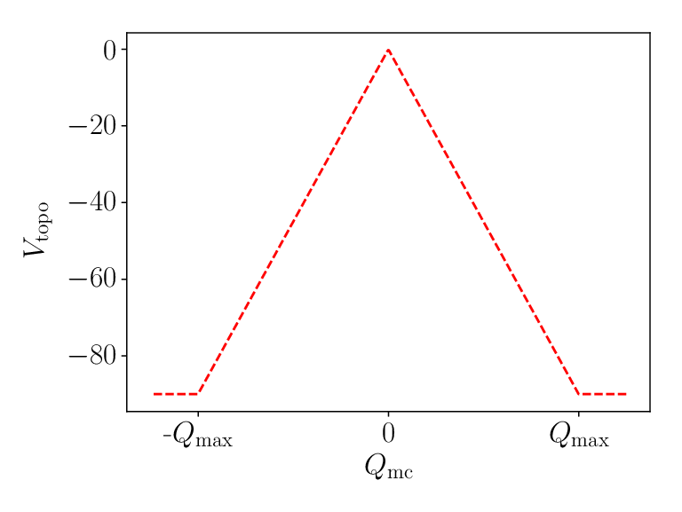
Our implementation of the multicanonic algorithm follows the lines of Ref. Jahn et al. 2018. First, we generate a candidate new lattice configuration by performing a standard updating step and ignoring the -dependent bias potential. Then, we accept the updated configuration by performing a standard Metropolis test:
where
is the variation of the bias potential before and after the update. After running some preliminary simulations, we found that the optimal implementation to have higher Metropolis acceptances was to perform the Metropolis test after each single-link update , instead of performing it after a whole standard MC step (i.e., after 5 sweeps of the whole lattice). Moreover, we also found that proposing single-site/single-link updates stochastically was more effective to obtain higher Metropolis acceptances than performing lattice sweeps.
It is easy to verify that, for any starting updating step, our choice respects detailed balance for the original distribution. Moreover, when considering the path-integral probability distribution obtained with the modified action in Eq. (24), our multicanonical updating step with the addition of the Metropolis test respects detailed balance too.
Finally, regarding the topological charge discretization , our choice is , i.e., the geometric definition in Eq. (13) computed without performing any cooling step. This choice allows to avoid the full computation of (necessary to compute the Metropolis probability) every time an update of a link variable is proposed, as with this choice one can directly compute in terms of the new link and its relative staples.
With this setup, we obtained mean Metropolis acceptances larger than , and we found that a multicanonical MC step required a larger numerical effort compared to a standard MC step. After taking into account such overhead, we found that the multicanonic algorithm allowed to gain up to two orders of magnitude in terms of computational power compared to the standard algorithm when .
References
- D’Adda et al. (1978) A. D’Adda, M. Lüscher, and P. Di Vecchia, Nucl. Phys. B 146, 63 (1978).
- Shifman (2012) M. Shifman, Advanced topics in Quantum Field Theory (Cambridge University Press, Cambridge, 2012), pp. 171–268, 361–367.
- Vicari and Panagopoulos (2009) E. Vicari and H. Panagopoulos, Phys. Rept. 470, 93 (2009), eprint 0803.1593.
- Witten (1980) E. Witten, Annals Phys. 128, 363 (1980).
- Witten (1998) E. Witten, Phys. Rev. Lett. 81, 2862 (1998), eprint hep-th/9807109.
- Rossi and Vicari (1993) P. Rossi and E. Vicari, Phys. Rev. D 48, 3869 (1993), eprint hep-lat/9301008.
- Rossi (2016) P. Rossi, Phys. Rev. D94, 045013 (2016), eprint 1606.07252.
- Campostrini and Rossi (1991) M. Campostrini and P. Rossi, Phys. Lett. B 272, 305 (1991).
- Campostrini et al. (1992a) M. Campostrini, P. Rossi, and E. Vicari, Phys. Rev. D 46, 2647 (1992a).
- Campostrini et al. (1992b) M. Campostrini, P. Rossi, and E. Vicari, Phys. Rev. D 46, 4643 (1992b), eprint hep-lat/9207032.
- Campostrini and Rossi (1993) M. Campostrini and P. Rossi, Riv. del Nuovo Cim. 16, 1 (1993).
- Bonati et al. (2016) C. Bonati, M. D’Elia, P. Rossi, and E. Vicari, Phys. Rev. D94, 085017 (2016), eprint 1607.06360.
- Bonanno et al. (2019) C. Bonanno, C. Bonati, and M. D’Elia, JHEP 01, 003 (2019), eprint 1807.11357.
- Berni et al. (2019) M. Berni, C. Bonanno, and M. D’Elia, Phys. Rev. D100, 114509 (2019), eprint 1911.03384.
- Forster (1977) D. Forster, Nucl. Phys. B130, 38 (1977).
- Berg and Lüscher (1981) B. Berg and M. Lüscher, Nucl. Phys. B 190, 412 (1981).
- Haldane (1983a) F. D. M. Haldane, Phys. Lett. A 93, 464 (1983a).
- Haldane (1983b) F. D. M. Haldane, Phys. Rev. Lett. 50, 1153 (1983b).
- Bhanot and David (1985) G. Bhanot and F. David, Nucl. Phys. B251, 127 (1985).
- Haldane (1985) F. D. M. Haldane, J. Appl. Phys. 57, 3359 (1985).
- Wiegmann (1985) P. B. Wiegmann, Phys. Lett. B 152, 209 (1985).
- Affleck and Haldane (1987) I. Affleck and F. D. M. Haldane, Phys. Rev. B 36, 5291 (1987).
- Hasenfratz et al. (1990) P. Hasenfratz, M. Maggiore, and F. Niedermayer, Phys. Lett. B 245, 522 (1990).
- D’Elia et al. (1995) M. D’Elia, F. Farchioni, and A. Papa, Nucl. Phys. B 456, 313 (1995), eprint hep-lat/9505004.
- D’Elia et al. (1997) M. D’Elia, F. Farchioni, and A. Papa, Phys. Rev. D55, 2274 (1997), eprint hep-lat/9511021.
- Blatter et al. (1996) M. Blatter, R. Burkhalter, P. Hasenfratz, and F. Niedermayer, Phys. Rev. D53, 923 (1996), eprint hep-lat/9508028.
- Burkhalter et al. (2001) R. Burkhalter, M. Imachi, Y. Shinno, and H. Yoneyama, Prog. Theor. Phys. 106, 613 (2001), eprint hep-lat/0103016.
- Controzzi and Mussardo (2004) D. Controzzi and G. Mussardo, Phys. Rev. Lett. 92, 021601 (2004), eprint hep-th/0307143.
- Alles and Papa (2008) B. Alles and A. Papa, Phys. Rev. D 77, 056008 (2008), eprint 0711.1496.
- Nogradi (2012) D. Nogradi, JHEP 05, 089 (2012), eprint 1202.4616.
- Azcoiti et al. (2012) V. Azcoiti, G. Di Carlo, E. Follana, and M. Giordano, Phys. Rev. D 86, 096009 (2012), eprint 1207.4905.
- Alles et al. (2014) B. Alles, M. Giordano, and A. Papa, Phys. Rev. B90, 184421 (2014), eprint 1409.1704.
- Bietenholz et al. (2018) W. Bietenholz, P. de Forcrand, U. Gerber, H. Mejía-Díaz, and I. O. Sandoval, Phys. Rev. D 98, 114501 (2018), eprint 1808.08129.
- Bruckmann et al. (2019) F. Bruckmann, K. Jansen, and S. Kühn, Phys. Rev. D 99, 074501 (2019), eprint 1812.00944.
- Sulejmanpasic and Tanizaki (2018) T. Sulejmanpasic and Y. Tanizaki, Phys. Rev. B 97, 144201 (2018), eprint 1802.02153.
- Sulejmanpasic et al. (2020) T. Sulejmanpasic, D. Göschl, and C. Gattringer, Phys. Rev. Lett. 125, 201602 (2020), eprint 2007.06323.
- Thomas and Monahan (2022) S. Thomas and C. Monahan, PoS LATTICE2021, 076 (2022), eprint 2111.11942.
- Marino et al. (2022) M. Marino, R. Miravitllas, and T. Reis (2022), eprint 2205.04495.
- Bonanno et al. (2021) C. Bonanno, C. Bonati, and M. D’Elia, JHEP 03, 111 (2021), eprint 2012.14000.
- Kitano et al. (2021a) R. Kitano, N. Yamada, and M. Yamazaki, JHEP 02, 073 (2021a), eprint 2010.08810.
- Kitano et al. (2021b) R. Kitano, R. Matsudo, N. Yamada, and M. Yamazaki, Phys. Lett. B 822, 136657 (2021b), eprint 2102.08784.
- Berni et al. (2020) M. Berni, C. Bonanno, and M. D’Elia, Phys. Rev. D 102, 114519 (2020), eprint 2009.14056.
- Del Debbio and Ramos (2021) L. Del Debbio and A. Ramos (2021), eprint 2101.04762.
- Berg and Neuhaus (1991) B. A. Berg and T. Neuhaus, Phys. Lett. B 267, 249 (1991).
- Jahn et al. (2018) P. T. Jahn, G. D. Moore, and D. Robaina, Phys. Rev. D 98, 054512 (2018), eprint 1806.01162.
- Bonati and D’Elia (2018) C. Bonati and M. D’Elia, Phys. Rev. E98, 013308 (2018), eprint 1709.10034.
- Bonati et al. (2018) C. Bonati, M. D’Elia, G. Martinelli, F. Negro, F. Sanfilippo, and A. Todaro, JHEP 11, 170 (2018), eprint 1807.07954.
- Athenodorou et al. (2022) A. Athenodorou, C. Bonanno, C. Bonati, G. Clemente, F. D’Angelo, M. D’Elia, L. Maio, G. Martinelli, F. Sanfilippo, and A. Todaro, JHEP 10, 197 (2022), eprint 2208.08921.
- Petcher and Lüscher (1983) D. Petcher and M. Lüscher, Nuclear Physics B 225, 53 (1983), ISSN 0550-3213.
- Lian and Thacker (2007) Y. Lian and H. B. Thacker, Phys. Rev. D75, 065031 (2007), eprint hep-lat/0607026.
- Lüscher (1982) M. Lüscher, Nucl. Phys. B 200, 61 (1982).
- Symanzik (1983) K. Symanzik, Nuclear Physics B 226, 187 (1983).
- Caracciolo and Pelissetto (1998) S. Caracciolo and A. Pelissetto, Phys. Rev. D 58, 105007 (1998), eprint hep-lat/9804001.
- Campostrini et al. (1988) M. Campostrini, A. Di Giacomo, and H. Panagopoulos, Phys. Lett. B212, 206 (1988).
- Farchioni and Papa (1993) F. Farchioni and A. Papa, Phys. Lett. B 306, 108 (1993).
- Berg (1981) B. Berg, Phys. Lett. B 104, 475 (1981).
- Alles et al. (1998) B. Alles, M. D’Elia, A. Di Giacomo, and R. Kirchner, Phys. Rev. D 58, 114506 (1998), eprint hep-lat/9711026.
- D’Elia (2003) M. D’Elia, Nucl. Phys. B661, 139 (2003), eprint hep-lat/0302007.
- Bonati and D’Elia (2014) C. Bonati and M. D’Elia, Phys. Rev. D89, 105005 (2014), eprint 1401.2441.
- Alexandrou et al. (2015) C. Alexandrou, A. Athenodorou, and K. Jansen, Phys. Rev. D92, 125014 (2015), eprint 1509.04259.
- Del Debbio et al. (2004) L. Del Debbio, G. M. Manca, and E. Vicari, Phys. Lett. B 594, 315 (2004), eprint hep-lat/0403001.
- Lüscher and Schaefer (2011) M. Lüscher and S. Schaefer, JHEP 07, 036 (2011), eprint 1105.4749.
- Hasenbusch (2017) M. Hasenbusch, Phys. Rev. D 96, 054504 (2017), eprint 1706.04443.
- Bonanno et al. (2022) C. Bonanno, M. D’Elia, B. Lucini, and D. Vadacchino, Phys. Lett. B 833, 137281 (2022), eprint 2205.06190.
- Altenkort et al. (2021) L. Altenkort, A. M. Eller, O. Kaczmarek, L. Mazur, G. D. Moore, and H.-T. Shu, Phys. Rev. D 103, 114513 (2021), eprint 2012.08279.