Chaumeny et al.
Bayesian nonparametric mixture inconsistency for the number of components: How worried should we be in practice?
Abstract
We consider the Bayesian mixture of finite mixtures (MFMs) and Dirichlet process mixture (DPM) models for clustering. Recent asymptotic theory has established that DPMs overestimate the number of clusters for large samples and that estimators from both classes of models are inconsistent for the number of clusters under misspecification, but the implications for finite sample analyses are unclear. The final reported estimate after fitting these models is often a single representative clustering obtained using an MCMC summarisation technique, but it is unknown how well such a summary estimates the number of clusters. Here we investigate these practical considerations through simulations and an application to gene expression data, and find that (i) DPMs overestimate the number of clusters even in finite samples, but only to a limited degree that may be correctable using appropriate summaries, and (ii) misspecification can lead to considerable overestimation of the number of clusters in both DPMs and MFMs, but results are nevertheless often still interpretable. We provide recommendations on MCMC summarisation and suggest that although the more appealing asymptotic properties of MFMs provide strong motivation to prefer them, results obtained using MFMs and DPMs are often very similar in practice.
keywords
Bayesian nonparametric analysis, Cluster analysis, Dirichlet process, Number of clusters, Mixture model.1 Introduction
Many areas of applied statistics use mixture models for cluster analysis. One advantage of this approach compared to heuristic counterparts is the possibility of inference on both individual cluster allocations and the entire clustering structure. Mixture models have been developed for a wide variety of data types, with applications to gene expression analysis (Medvedovic and Sivaganesan 2002; McLachlan et al. 2002; de Souto et al. 2008; Onogi et al. 2011; Crook et al. 2018), economics (Alfò et al. 2008; Wedel and Desarbo 2002; Frühwirth-Schnatter et al. 2004), cell type classification (Chan et al. 2008; Prabhakaran et al. 2016), community detection (Geng et al. 2019; Legramanti et al. 2021), climate science (Gaffney et al. 2007), astrophysics (Mukherjee et al. 1998), health surveys (Ni et al. 2020), demographics (Carmona et al. 2019) and finance (Dias et al. 2015). Reliable estimation of the number of clusters is essential for accurate prediction and decision-making—for example, precision medicine relies on identifying disease subtypes (Sørlie et al. 2001; Lanza and Rhoades 2013)—and various approaches to this have been developed (Dudoit and Fridlyand 2002; James et al. 2001; Nobile 2004; Woo and Sriram 2006; Henna 2008; Celeux et al. 2019).
Frequentist estimation of the number of clusters is commonly treated as a model selection problem, approaches to which include likelihood ratio tests (McLachlan 1987), information criteria (Biernacki et al. 2000; Celeux et al. 2006; Drton and Plummer 2017) and overfitting with penalised likelihood mixture models (Manole and Khalili 2021). Identifiability issues are a major difficulty in both Bayesian and frequentist formulations (Liu and Shao 2003); see Celeux et al. 2019 for an overview of the latter.
Bayesian mixture models treat the number of clusters as an unknown parameter for which principled uncertainty estimates may be obtained. We consider the mixture of finite mixtures (Nobile 2004; Miller and Harrison 2018) and Dirichlet process mixture models (MacEachern 1994; Escobar and West 1995; Neal 2000), two common extensions of the finite mixture model that allow inference for the number of clusters. The first benefits from consistency results (Nobile 1994), but estimation methods were inefficient until recently (Miller and Harrison 2018). The second is a nonparametric model that has become popular due to the existence of efficient estimation algorithms (Neal 2000; Jain and Neal 2004).
Despite their attractions, recent theory has established that estimators of the numbers of clusters based on these models have undesirable asymptotic properties. Dirichlet process mixtures have been shown to give inconsistent estimators of the number of clusters, overestimation of which has been observed for finite samples due to the appearance of small extra clusters (Miller and Harrison 2014). Mixtures of finite mixtures have been suggested as a consistent alternative, but model misspecification can still result in inconsistency and poor estimation of the number of clusters in practice (Cai et al. 2021). Moreover, high-dimensional data are particularly challenging for all clustering methods, which often incorrectly estimate the number of clusters (Chandra et al. 2021).
Although unsettling, poor asymptotic properties need not entail major problems in practical situations with finite samples, and our first aim in this work is to investigate to what extent the asymptotic results sabotage the estimation of the number of clusters with Bayesian mixtures models with sample sizes that are typical for applications.
In practice inference is generally performed using Markov chain Monte Carlo (MCMC) algorithms (Neal 2000). This results in a large number of MCMC samples of cluster allocations, which cannot be interpreted directly owing to the presence of multiple modes over all the partitions of the data, changes in the number of components, and label switching, so summarisation methods have been introduced to find a representative clustering (Binder 1978; Medvedovic et al. 2004; Fritsch and Ickstadt 2009; Wade and Ghahramani 2018; Rastelli and Friel 2018; Dahl et al. 2021). To summarise MCMC samples despite label switching (Jasra et al. 2005), these post-processing methods are often based on Bayesian decision theory, that is, they minimise the posterior expectation of a suitable loss function. The different choices among all possible combinations of loss function and optimisation method have led to the use of various summaries (Huelsenbeck and Andolfatto 2007; Savage et al. 2010; Kirk et al. 2012; Lock and Dunson 2013; Roth et al. 2014; Yuan et al. 2015; Carmona et al. 2019; Zafar et al. 2019; Fuentes-García et al. 2019; Ni et al. 2020), but the effect of summarisation methods has not yet been studied, especially with regard to the summarising number of clusters, which need not be representative of the corresponding marginal posterior distribution. Hence a second goal of our work is to investigate how the summarisation method affects the number of clusters in light of the theoretical results. We focus on the low-dimensional case to avoid complications that can arise with clustering methods and MCMC samplers in high dimensions.
Another popular approach to estimating the number of components is overfitting with finite mixture models. By deliberately fitting a model with an upper bound on the number of components we can estimate the true number of clusters by discarding empty components. Rousseau and Mengersen 2011 show that overfitting can give consistent estimators , and that additional components vanish a posteriori at rate for some . We do not consider this approach, which requires setting parameter which should be higher than the unknown , and for high enough, this model is comparable to a Dirichlet process mixture (Frühwirth-Schnatter and Malsiner-Walli 2019).
Non-decision-theoretic approaches intended to correct Dirichlet process mixture overestimation of the number of components also exist. For instance, Guha et al. 2019 introduce an algorithm that merges small additional clusters of each MCMC sample in post-processing. They prove that their method is consistent for the number of components, but it involves a model-specific theoretical contraction rate to adjust the truncation of small clusters; they provide this rate for Gaussian mixture models. We do not consider such algorithms, because decision theory-based summaries are more common in practice.
In Section 2, we introduce the types of Bayesian mixture models that we consider, summarise known asymptotic (in)consistency results and present different strategies for summarising simulation output for these models. We perform a study on synthetic data in Section 3 and illustrate the results using gene expression data. We conclude by discussing our results and give an overview of alternative approaches and potential future work.
2 Background, theory and summarisation methods
2.1 Bayesian mixture models
2.1.1 Finite mixture model
Mixture models presuppose that the data are generated from a mixture of component distributions belonging to a given parametric family, and clusters are determined by observations generated by the same component. A Bayesian finite mixture model for observations with components can be defined hierarchically as
| (1) | ||||
where the component distribution is parameterised by and is a prior distribution on the component parameters. The component allocations indicate the component responsible for each observation, while the vector represents the component proportions (also called the mixing distribution), i.e., is interpreted as the prior probability that an observation belongs to component . The prior on is here taken to be a symmetric Dirichlet distribution with a parameter commonly set to or . By marginalising over , the probability density function of an observation can be written as
| (2) |
where is the component probability density function associated with . Thus, we recover the standard representation of a mixture.
The most common choice of component distribution for continuous data is multivariate Gaussian. For variables this corresponds to setting such that for , where is a vector and is a positive semi-definite matrix.
2.1.2 Mixture of finite mixtures model
A natural extension of the finite mixture model (1) is to treat the number of components as an unknown parameter with a prior . The resulting mixture of finite mixtures (MFM) model can be defined hierarchically as
| (3) | ||||
If we set we recover a finite mixture model with components. The mixture of finite mixtures model is sometimes also called a finite mixture model with a prior on the number of components (Nobile 1994; Richardson and Green 1997). Some examples of discrete priors are a Poisson distribution for (Nobile 2007) or a Geometric distribution (Miller and Harrison 2018).
2.1.3 Dirichlet process mixture model
Another extension of the finite mixture model is the Dirichlet process mixture model, under which each observation has an associated parameter, , with assumed to be independent and identically distributed according to a random distribution . The prior on is a Dirichlet process, , where is the concentration parameter and is the base measure. The Dirichlet process mixture (DPM) model can therefore be written hierarchically as
| (4) | ||||
A practical definition of the resulting distribution of is provided by the Pólya urn scheme (Blackwell and MacQueen 1973).
In contrast to the MFM, under which the prior density of the number of components is fixed as , the Dirichlet process prior allows an increasing number of components as the number of observations grows. Indeed, the prior expectation of , the number of components for or equivalently the number of unique values of , satisfies
| (5) |
For more properties of the Dirichlet process see Ghosal 2010, for example.
2.2 Known asymptotic properties
There are various theoretical results for the estimation of the number of components with Bayesian mixture models. In general we present asymptotic results as the number of observations tends to infinity. Due to the generality of mixture models, useful results require further assumptions, but these hold in most practical settings and in particular for those we study in Section 3.
Although we focus on component allocation and the number of components, an underlying issue is density estimation: although the posterior number of components may be inconsistent, the mixture density can still converge to the true generating density. Nguyen 2013, for example, shows that the posterior distribution of a DPM model converges to the true distribution in the Wasserstein metric, and Guha et al. 2019 show that the posterior distribution of a MFM model contracts to the true generating parameters at an optimal rate under correct specification, up to relabeling of the components. These authors also show that even under misspecification both types of models can asymptotically recover the true parameters under certain conditions. Under an identifiability condition on the true generating distribution, they show in particular that a multivariate normal mixture distribution converges in the Wasserstein metric, though the convergence is slower than for the well-specified case. However, as we describe in Section 2.2.3, under misspecification the estimated number of components is inconsistent and diverges. This is a recurring trade-off for mixture models: it is possible to obtain an arbitrarily good density estimate, but at the cost of overestimating the number of components.
2.2.1 Consistency of mixture of finite mixtures
For the mixture of finite mixtures model, Nobile 1994 shows that the posterior converges to the true number of components, if the mixture is identifiable and the component distribution is continuous. Mixture-identifiability means that a mixture of components is strictly more expressive than any mixture with components and it is uniquely identified up to relabeling of the components. Many models satisfy this condition, including Gaussian mixtures and most common continuous component distributions.
2.2.2 Inconsistency of Dirichlet process mixture
Miller and Harrison 2014 show that the posterior distribution of the number of components of a Dirichlet process mixture, or more generally a Pitman–Yor mixture model does not contract to the true number of components when the observations arise from a finite mixture. However it is still unclear what the posterior distribution actually does, for instance, it might contract around a wrong value, or diverge entirely. Yang et al. 2020 show that the posterior diverges when a uniform or Gaussian prior is taken for . Since we do not know the convergence speed it is difficult to assess the finite-sample repercussions of this, and other aspects such as the choice of may be more important when is finite. In fact, Miller and Harrison 2014 do not cover the case where is also a parameter with a hyperprior, though they suspect their result to hold regardless. However, more recent work has shown that consistency can be achieved by putting a prior on (Ascolani et al. 2022), or allowing it to depend on the sample size (Ohn and Lin 2022), although it is unclear whether these results hold for mixtures of multivariate Gaussian densities with unknown covariance matrix, which are most commonly used for clustering.
2.2.3 Inconsistency under misspecification
The consistency result for the mixture of finite mixtures model in Section 2.2.1 holds when the generating and modelling component distribution families are the same, but we may ask whether it remains true under misspecification, which is frequent, perhaps even invariable, in practice. We saw in Section 2.2.2 that misspecification of the allocation prior can lead to inconsistency. Cai et al. 2021 show that mixtures of finite mixtures with misspecified component distributions are also inconsistent for the number of components. Indeed, they show that the posterior diverges for any misspecified location-scale family of component distributions, if the corresponding mixture is identifiable and absolutely continuous with respect to the parameter , and the data generating mixture lies in the Kullback–Liebler support of the prior. Under an assumption of degenerate limits they also prove a more general statement for any continuous density/mass function.
2.3 Summarisation of MCMC samples
Analytic computations for Bayesian mixture models are intractable, so the usual approach is to use Markov chain Monte Carlo (MCMC) sampling, which results in a time series from the posterior , where is chosen adequately large in practice. Even if the are sampled from the exact posterior distribution, the results cannot be interpreted directly using sample averages or other standard summary statistics owing to two major identifiability issues for the components, namely label-switching and variation in the number of components.
Label-switching creates an incoherence in the values of the posterior samples of . Any permutation of the component labels leaves the posterior density unchanged, so taking a summary clustering, such as the average of the samples, is not helpful, because two samples and may represent the same component allocation with permuted labels: with and , for example, the labelings and lead to the same clustering. Moreover, the number of components vary during sampling, further complicating the challenge of summarisation.
Formally, a summarisation method is a function from to a single summary clustering of the observations, i.e.,
| (6) | ||||
Figure illustrates the summarisation task and shows the difference between the posterior number of components and the number of clusters of a summary clustering. Post-processing methods are intended to provide a “representative” . The concept of representativity is not uniquely defined, but Binder 1978 introduced a formal definition within a loss minimisation framework. For most summarisation methods we can define a loss function such that
| (7) |
where the expectation is taken over . In order that the loss be invariant to relabeling, clusterings should be treated as partitions of the set , and then a direct MCMC approximation of (7) is
| (8) |
A central quantity for post-processing samples is the posterior similarity matrix (PSM) with elements
| (9) |
where is the indicator function, which measures the frequency of co-clustering of pairs of observations and is invariant to label-switching or to changes in the numbers of components during sampling. To simplify notation in this section we write for the number of clusters in and denote the contingency counts of two clusterings and K(z) ×K ( ^ z )
2.4 Loss functions
2.4.1 Maximum a posteriori
A straightforward approach to obtaining a summary clustering is to take the sample that maximizes the unnormalised posterior density. This corresponds to taking the 0-1 loss in (8), i.e., where is defined up to relabeling. This entirely circumvents the label switching problem by only considering a single sample, rather than comparing clusterings with possibly different labelings.
2.4.2 Binder’s loss
The first loss function for summarising MCMC samples is due to Binder 1978, which uses pairwise co-clustering disagreement to measure differences between two clusterings via
| (11) |
where are commonly set to , though other values could be used in case of asymmetric classification error. We set , but Dahl et al. 2021 show that changing the ratio can significantly affect the number of clusters.
The expected posterior loss can be written in terms of the posterior similarity matrix as
| (12) |
Binder’s loss has a direct relationship with the commonly-used Rand index (Rand 1971). Indeed, for ,
| (13) |
so minimising the expected posterior Binder loss is equivalent to maximising the expected posterior Rand index.
2.4.3 Posterior Expected Adjusted Rand (PEAR)
Fritsch and Ickstadt 2009 propose using the summary clustering that maximises the posterior adjusted Rand index (Hubert and Arabie 1985). While they do not explicitly introduce a loss function, we define the adjusted Rand loss as
| (14) |
where the adjusted Rand index AR corrects the Rand index for chance under permutations within clusters. For computational reasons Fritsch and Ickstadt 2009 suggest taking the approximation in AR, but Dahl et al. 2021 argue that this is unnecessary and may lead to inaccuracies. Nevertheless, we will use the approximate optimisation, as it is typically used in practice.
2.4.4 Variation of Information
A loss function can also be based on a distance metric on the space of clusterings. Wade and Ghahramani 2018 suggest using as a loss function the variation of information (Meila 2007), which has the advantage of inheriting theoretical properties from the distance space. The variation of information distance between two clusterings is
| (15) | ||||
where is called the entropy and is the joint entropy for cluster allocations. Intuitively, this distance is small if the amount of information two clusterings share, captured by the joint entropy, is close to the individual information of each clustering, captured by their entropy.
The posterior expectation of by (8) involves , computation of which requires the contingency counts for each sample. Instead, Wade and Ghahramani 2018 find a lower bound on the posterior expected loss, which only requires the computation of the posterior similarity matrix and leads to the loss function
| (16) |
where we omit terms that do not depend on . We use the lower bound approximation in our implementation.
2.5 Optimisation
Loss optimisation over all possible clusterings is infeasible for computational reasons. Indeed, if is the set of all clusterings of , then grows very rapidly as a function of . The number of partitions into two clusters is , so a simple lower bound is , indicating that optimisation of the loss function is NP-hard and it is necessary to consider a reduced set of clusterings. We approximate the optimisation as
| (17) |
where . In the following subsections we consider various choices of .
We also mention more recent optimisation methods that we do not consider for brevity. Rastelli and Friel 2018 use a greedy search algorithm and avoid computing the posterior similarity matrix, which is a costly intermediate step when is large, but nevertheless require certain types of loss functions which can be updated efficiently when a single is changed. Dahl et al. 2021 extend this optimisation algorithm with parallel programming and further search steps. However, these two approaches have not yet found wide use in practice, so we restrict ourselves to popular methods.
2.5.1 Hierarchical clustering
A common post-processing approach is to convert the posterior similarity matrix into a metric between any two observations and then apply standard hierarchical clustering methods (Medvedovic et al. 2004; Fritsch and Ickstadt 2009). For this we define the posterior dissimilarity matrix as for , and perform agglomerative clustering on with either complete or average linkage.
Denoting the cluster allocation with clusters by , Fritsch and Ickstadt 2009 suggest optimising the loss function in (17) with for some upper bound such as . If the posterior similarity matrix is already computed, this approach is very efficient, as we can update the linkage distances in constant time at every merging step, for a total of operations. However, this yields only a single element of per value of , whereas a desirable property of would be concentration around an appropriate numbers of clusters.
Medvedovic et al. 2004 introduced hierarchical clustering without loss function optimisation, instead obtaining directly as the clustering that exceeds a linkage distance across any pair of clusters. Fritsch and Ickstadt 2009 suggest , which we consider as a default. Unlike other methods we present, Medvedovic clustering does not depend on a loss function and does not seem to be expressible in decision-theoretic terms.
2.5.2 Partitioning around medoids
Liverani et al. 2015 suggest optimisation using the popular -medoids algorithm, which generalises -means for any metric. More precisely, they use as a distance metric and choose partitioning around medoids as an efficient implementation of -medoids. Kaufman and Rousseeuw 1990 improve this approach by instead successively swapping medoids to minimize a global cost function. Nonetheless, when is large, partitioning around medoids is also inefficient as it requires iterations. We may therefore consider more efficient approaches such as that of Schubert and Rousseeuw 2019.
By denoting the output clustering of k-medoids with clusters by , Liverani et al. 2015 suggest optimising the loss function in (17) with for some upper bound . We choose in our implementation.
2.5.3 Sample search
A straightforward choice for is the set of MCMC samples (Dahl 2006). The resulting summary clustering is a posterior sample , which also provides associated sample component parameters . However, if all samples inherit an undesired property from the sampling method or the model itself, such as overestimation of the number of components, the summary clustering will also have this property.
3 Evaluation
We now summarise the results of our analysis applying MFMs and DPMs, with and without conjugate hyperpriors on the component parameters, and with different summarisation methods. We use three scenarios with simulated data and one with real data.
The first scenario corresponds to a sample with a moderate sample size for which MFMs and DPMs are similar. Since the marginal posteriors for the number of clusters are highly concentrated at the truth, this easy case sets a baseline for comparing the different summarisation methods.
The second scenario corresponds to a larger sample size at which the DPM and MFM start to differ and which is more challenging for the summarisation methods. We focus on the DPM with hyperpriors since the corresponding posterior for the number of clusters is the flattest, with a mode that is higher than the truth in some of the simulated datasets.
The third scenario is used to explore how a common type of misspecification affects summarisation methods, by modelling correlated data using multivariate Gaussian components with diagonal covariance matrices.
Finally, we show results for the gene expression dataset used in Cai et al. 2021, where we expect to observe both the effects of DPM inconsistency and of misspecification. Again, we compare the outcomes of the different summarisation methods and use cell types as a proxy for true labels.
3.1 Modelling specification
We consider continuous data and multivariate normal mixture models. In the multivariate models we consider either a model with full covariance matrix or one with a diagonal covariance matrix. Both assumptions are common in practice, and in particular the restriction to a diagonal covariance has valued computational advantages. The component distributions with a full covariance specification are
| (18) | ||||
where is the sample mean, is the sample covariance and is the component index. As it is common to include hyperpriors to give models more flexibility or to incorporate prior assumptions, we also consider an alternative model with conjugate hyperpriors on the component parameters, i.e.,
| (19) | ||||
For the diagonal covariance model we standardize the observations beforehand, so our modelling assumptions can rely on standardised data. Hence, we have
| (20) | ||||
for each dimension independently.
We consider two types of allocation prior, either a mixture of finite mixtures (3) or a Dirichlet process mixture (4). For the first, and , following Miller and Harrison 2018. For the second, .
For both models we obtain MCMC samples with the split-merge sample with four independent chains, each with iterations, and the first iterations removed as burn-in. We thin the MCMC samples by keeping every second iteration, giving samples in total. Miller and Harrison 2018 show fast convergence of the split-merge sampler, so we choose the sample size sufficiently large to be representative while limiting the running time. We assess convergence using the Geweke and the Gelman–Rubin diagnostics across multiple chains (Geweke 1991; Gelman and Rubin 1992; Vehtari et al. 2020).
3.2 Simulation study
In order that the true number of components is known, we generate synthetic data using a finite mixture model from Miller and Harrison 2018 with four clusters. Our synthetic bivariate observations are distributed as
| (21) | ||||
where
| (22) |
3.2.1 Moderate sample size
To obtain representative results we generated independent datasets with observations from model (21). Figure 2 shows one of these datasets, which display overlap between the component densities. Uncertainty between clusters is often seen in applications, so by fixing , and we control the difficulty of the clustering task. If instead we generate data from the model with hyperpriors, then we do not control distances between component means, which may confound our interpretation of results.
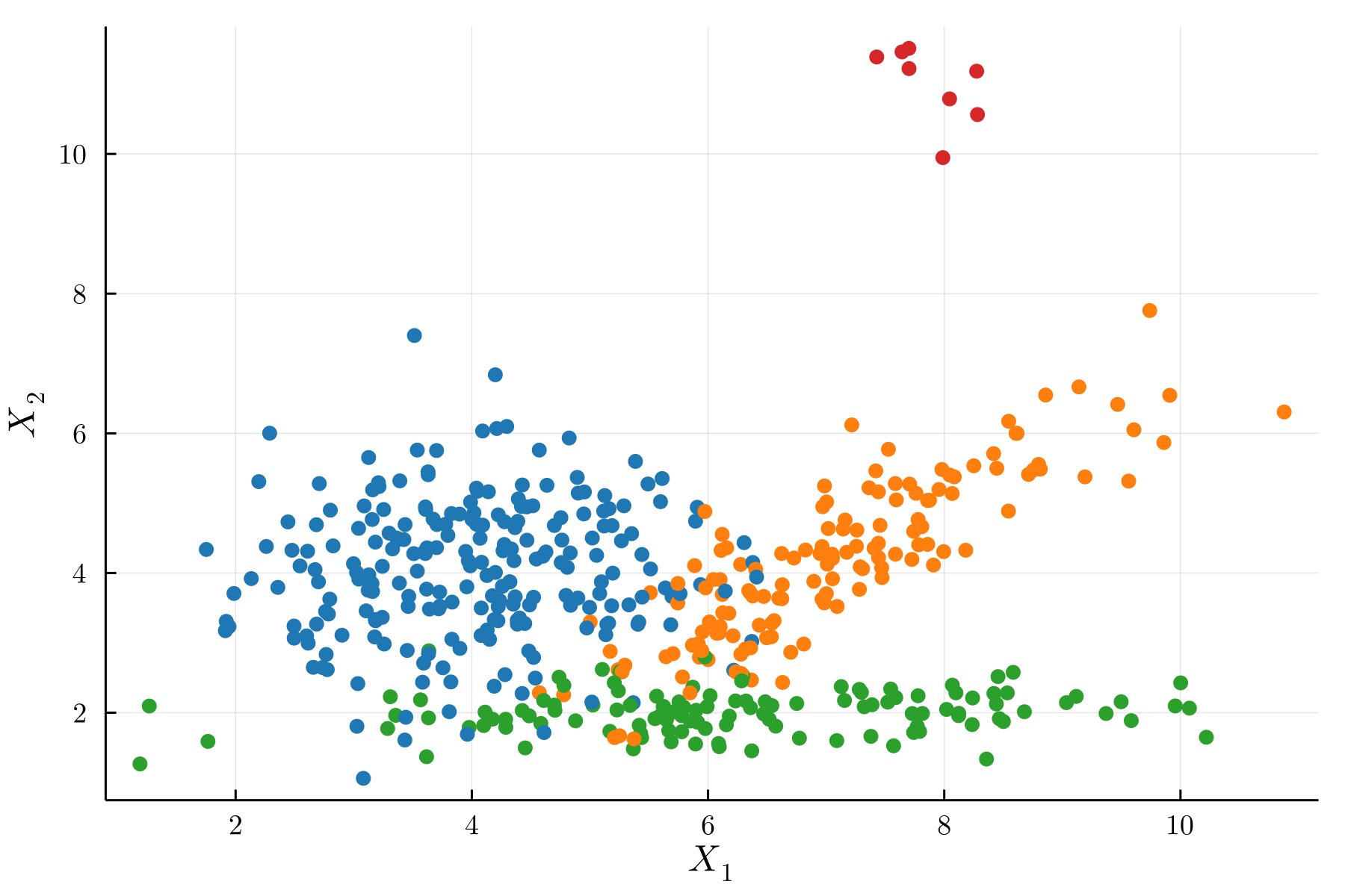
We perform estimation with the full covariance models (18) and (19) and four model types: the mixture of finite mixtures with and without a hyperprior on the parameters of the mixture components and the Dirichlet process mixture with and without hyperpriors, which we respectively abbreviate to MFMH, MFM, DPMH and DPM. At each iteration we obtain a sample of component allocations and the number of active components .
Figure 3 shows every resulting posterior on the number of components. For clarity, we maintain a consistent colouring of the four model types in all following figures. To obtain the posterior of for the mixture of finite mixtures model, we use the posterior on given the number of active components , provided by Miller and Harrison 2018. Although the dataset in Figure 2 is well-specified by the full covariance model and is a moderate sample size, there are differences between the model types: the hyperpriors seem to flatten the posterior number of components towards higher values, and the Dirichlet process mixture allows exploration of higher numbers of components during MCMC sampling.
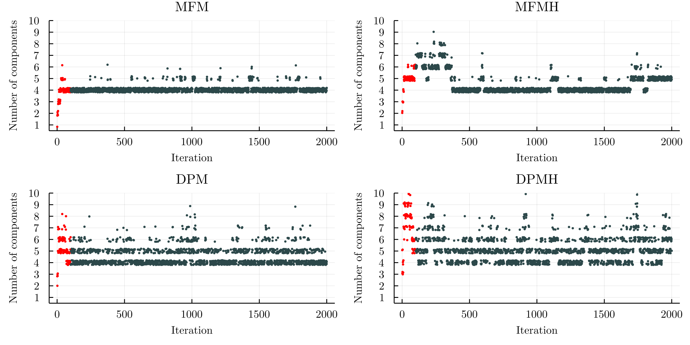
The identifiability issues make diagnostics for MCMC samples of , and challenging, and we can only consider the number of components or . Figure 13 in the Appendix gives an example of the number of components for a single chain before thinning and including the burn-in samples when fitting each of our models to the data shown in Figure 2.


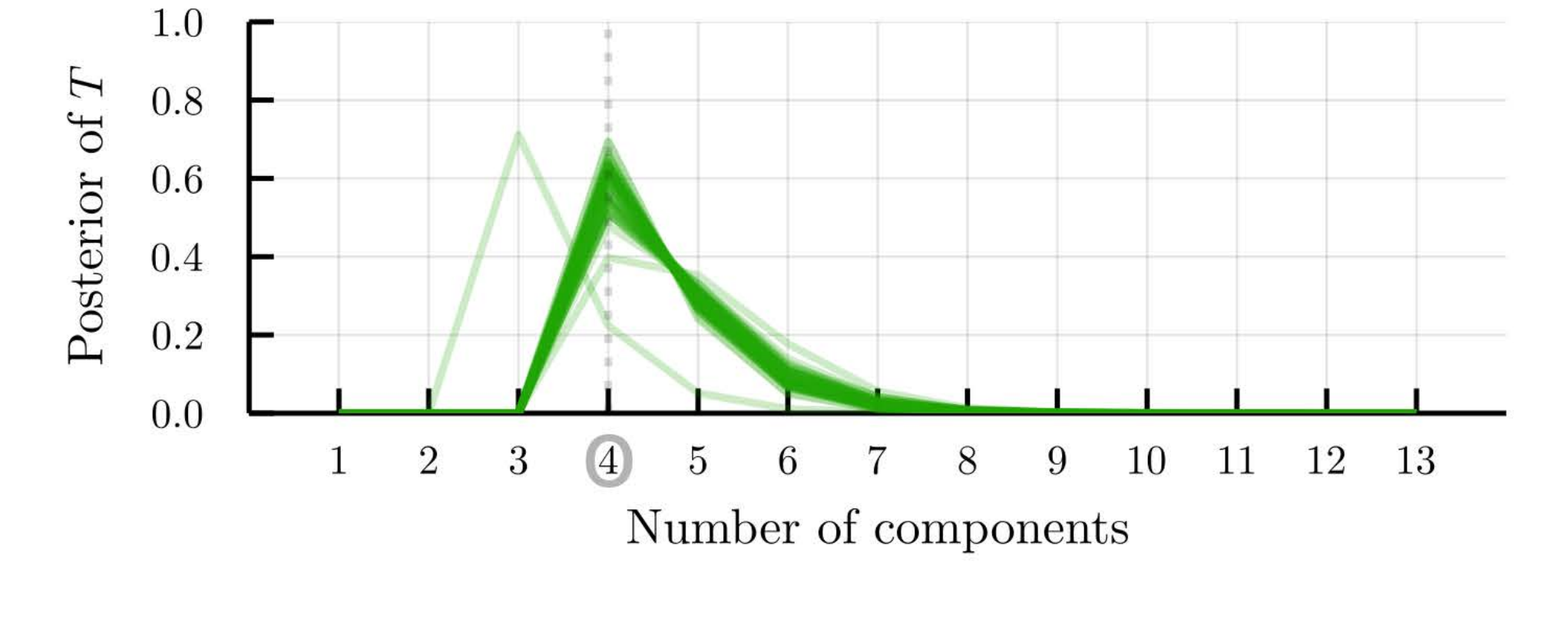

For every dataset and model type we derive the summary clusterings described in Section 2.2.3, each of which gives a number of clusters. As an example, Figure 4 summarises the results for the mixture of finite mixtures model without a hyperprior. The posteriors at the right are those in Figure 3. The summarisation methods with a loss function are Binder’s loss (Binder), the posterior expected adjusted Rand index (PEAR), the lower bound of the variation of information (VI-LB), average and complete linkage hierarchical clustering (Average and Complete), sample search (Samples) and partitioning around medoids (PAM). Although this case is rather simple, some methods vastly overestimate the number of clusters.

Our main focus is the number of clusters, but this is linked to the underlying cluster allocations. Nonetheless, an accurate clustering can coexist with an inaccurate number of clusters, at least when accuracy is measured with popular scores such as the adjusted Rand index. The addition of small clusters has a minor impact on these scores provided the large clusters are correctly identified, as illustrated in the Appendix; see Figure 14.
3.2.2 Dirichlet process mixture inconsistency
To investigate the Dirichlet process mixture and asymptotic results of Section 2.2.2 we set . We consider the Dirichlet process mixture with hyperpriors, as it shows the highest overestimation of the number of components even when , and in Figure 5 show the posterior number of components for independent datasets. The Dirichlet process mixture model tends to overestimate the number of components, in particular compared to the mixture of finite mixtures model.


The Dirichlet process mixture model tends to introduce small extra clusters, as noticed by Miller and Harrison 2014 and illustrated in Figure 15 in the Appendix.
Figure 6 gives the number of clusters for a selection of summary clusterings. We exclude results for Binder’s loss and PEAR loss with average linkage, which can both massively overestimate the number of clusters, and we do not use partitioning around medoids because of its much longer running time when is large. As expected, optimisation with sample search tends to follow the posterior distribution and leads to overestimation of the number of clusters, whereas Medvedovic clustering and variation of information both give the correct number of clusters for all datasets. This confirms that summary clustering methods may eliminate any small extra clusters introduced by the DPM model. Indeed, this holds even for data whose posterior mode is appreciably larger than four and the posterior credibility of four components is low.
Figure 16 of the Appendix gives two examples of summary clusterings; PEAR loss with average linkage is representative of methods not included in Figure 6, as it gives clusters, while variation of information leads to four clusters only. Both Binder’s loss and PEAR loss with complete linkage optimisation tend to create small clusters in the overlaps between components. This occurs independently of the model type, so it is a different phenomenon from Dirichlet process mixture inconsistency; indeed, Wade and Ghahramani 2018 already notice this for Binder’s loss. Our results in Section 3.2.1 show that Binder’s loss leads to poor results for the number of clusters that for . For PEAR loss we could investigate whether the approximation by Fritsch and Ickstadt 2009 is the reason for these additional clusters. Variation of information successfully adjusts for small extra clusters introduced during sampling, but the resulting clustering differs from the generating component allocation, as the clusters do not have Gaussian shapes. We conjecture that the borders between clusters approximate the contour lines of equal component densities, e.g., , which would explain the straight boundaries between clusters.

3.2.3 Misspecification inconsistency
We now model the previous correlated data with using the diagonal covariance model (20), which is popular for computational reasons, to investigate asymptotic results from Section 2.2.3. The model (20) is misspecified, because it cannot express the correlation from . Indeed, with this choice we can specify a conjugate prior on the component distributions and sample directly from the component prior, thereby avoiding the conditional Gibbs update during the split-merge algorithm. Moreover the number of covariance parameters reduces from to for every component, so sampling should be more stable in high-dimensional cases.
We again generate datasets of correlated Gaussian mixture observations and sample from the diagonal covariance model (20). Figure 7 shows the posterior numbesr of components for two model types we consider. The MFM model gives concentrated posterior distributions for the number of components that contract onto a single value, though this varies across datasets. It is unclear why the model is sensitive to data generation, as we would expect almost identical data when is so large. MCMC samples, not shown here, show the creation of nearly identical overlapping components sharing observations of the well-specified components. One reason for this could be that, as gets large, the symmetric Dirichlet prior attributes more density to allocations with similar proportions, thereby giving potentially lower posterior credibility to uneven proportions. To investigate this we could choose a smaller , such as . The DPM model posterior distributions also vary across datasets, but are less concentrated than those for the MFM model. This difference may arise because of the overestimation described in Section 3.2.2.


Figure 8 shows the numbers of clusters for summarisation methods for the MFM and DPM models. As in the previous section, we omit methods with significant overestimation. Overall summary clusterings seem to minimise the number of components compared to the posterior but they do not recover the true number of components. Among these methods, variation of information leads to the most consistent reduction, giving seven clusters in most cases independently of the model type. Sample search optimisation seems to follow the posterior distribution. The adjusted Rand index of summary clusterings, not shown here, is similar for all methods except for the slightly less accurate sample search, similarly to Figure 14.


The only component that cannot be expressed using the diagonal covariance model is the second component. As is non-diagonal, the misspecified model introduces additional components. Figure 9 shows an MCMC sample selected by the variation of information loss in which four components approximate the second component. The summary clustering with hierarchical clustering optimisation inherits the three additional components from the MCMC samples. It seems that summary clusterings do not adjust for misspecification in this example, but only avoid small additional clusters, in particular for the DPM model.


3.3 Gene expression data
We now consider gene expression data from single-cell RNA sequencing of somatosensory cells (Zeisel et al. 2015), which have to address asymptotic theory, and which were also used by Cai et al. 2021 to illustrate the inconsistency result presented in Section 2.2.3. The data are 19,972 gene measurements from 3005 cells with seven cell types. We pre-process the data following Prabhakaran et al. 2016 and use the genes with the largest standard deviations because we aim to use our full covariance model in addition to the the diagonal covariance model used by Cai et al. 2021; Prabhakaran et al. 2016 took . Modelling using the full covariance model is much slower for large due to the additional correlation parameters, but sampling from both allows us to compare the diagonal covariance and more expressive full covariance models, though even the latter can be expected to be misspecified. According to Zeisel et al. 2015, there are seven known cell types, which we will consider as ground truth.
Figure 10 gives the posterior distributions of the number of components for models (18) and (20). The MFM and DPM models give similar posteriors for the full covariance model, with a mode at eight components, suggesting that the DPM overestimation of the number of components tends to be moderate for sample sizes in the order of and confirming our results in Section 3.2.2. The MFM posterior gives slightly more credibility to higher numbers of components than does that of the DPM. The diagonal covariance specification leads to a significant overestimation of the number of components, confirming the theoretical results from Section 2.2.3 and our simulation results in Section 3.2.3. Furthermore, the DPM model contributes to the overestimation of the number of components, with a mode at 18 components compared to 16 for the MFM model. Both model types show bimodal posterior distributions with a second local mode and have similar shapes, though the DPM posterior is shifted towards higher numbers of components.


Table 1 gives the number of clusters of summarisation methods. We do not consider methods based on partitioning around medoids due to computational limitations. Overall we confirm our simulation results, with overestimation of the number of clusters for Binder and PEAR losses with hierarchical clustering, especially with average linkage. Medvedovic clustering and variation of information correct the overestimation of the Dirichlet process mixture model with diagonal covariance, giving numbers of clusters similar to the MFM model. However, as in Section 3.2.3, summarisation methods do not correct the overestimation due to misspecification. The adjusted Rand indices show that the full covariance model is more accurate than the misspecified diagonal covariance model. We cannot expect perfect recovery of the true seven cell types, even with the full covariance model, because we use a very general model without consideration of the data type and without further prior assumptions.
| Number of clusters | Adjusted Rand index | |||||||
| Full | Diagonal | Full | Diagonal | |||||
| MFM | DPM | MFM | DPM | MFM | DPM | MFM | DPM | |
| Medvedovic | 8 | 8 | 15 | 16 | 0.38 | 0.35 | 0.34 | 0.35 |
| Binder+Average | 30 | 36 | 59 | 55 | 0.38 | 0.38 | 0.33 | 0.33 |
| Binder+Complete | 11 | 12 | 19 | 17 | 0.38 | 0.38 | 0.34 | 0.35 |
| Binder+Samples | 9 | 9 | 15 | 18 | 0.37 | 0.38 | 0.34 | 0.34 |
| PEAR+Average | 25 | 29 | 33 | 32 | 0.38 | 0.38 | 0.33 | 0.33 |
| PEAR+Complete | 11 | 12 | 18 | 17 | 0.38 | 0.38 | 0.34 | 0.35 |
| PEAR+Samples | 9 | 9 | 15 | 18 | 0.37 | 0.38 | 0.34 | 0.34 |
| VI-LB+Average | 9 | 8 | 14 | 15 | 0.38 | 0.38 | 0.33 | 0.35 |
| VI-LB+Complete | 9 | 9 | 15 | 15 | 0.38 | 0.38 | 0.34 | 0.35 |
| VI-LB+Samples | 9 | 8 | 15 | 19 | 0.37 | 0.37 | 0.34 | 0.33 |
| Posterior mode | 8 | 8 | 16 | 18 | ||||
| Truth | 7 | 7 | 7 | 7 | ||||
We use the Uniform Manifold Approximation and Projection (UMAP) (McInnes et al. 2020) to visualise our clusterings. Figure 11 illustrates summary clusterings for the MFM model on a two-dimensional projection of our data, which we compare to the true clustering according to Zeisel et al. 2015. The misspecified model seems to create subclusters of the full covariance, i.e., the clusters of the diagonal covariance model seem to split up the larger clusters of the full covariance model. For synthetic data, we showed in Section 3.2.3 that the diagonal covariance model splits up clusters with correlated data. We confirm our conjecture in Figure 12 by visualising the contingency counts for summary clusterings of the MFM model. By reordering the clusters of the diagonal covariance model, we roughly split up clusters of the full covariance model (rows) into clusters of the diagonal covariance (columns). For example, cluster 1 of the full diagonal covariance model can be split into clusters 4, 1 and 6 of the diagonal covariance model.


In conclusion, our analysis of the mouse single-cell RNA-sequence data confirms some of our simulated results. Misspecification of the component distributions seems to have a bigger effect on the overestimation of the number of components than does the Dirichlet process prior. Summarisation methods can correct the overestimation of the DPM model compared to the MFM model but they do not correct for misspecification of the component distributions. However, misspecification of Gaussian component distributions seems to split components of their well-specified counterpart, giving reasonably interpretable summary clusterings.
4 Discussion
Our simulation results confirm theoretical inconsistencies for the number of components of Bayesian mixture models from recent literature for finite samples. MCMC summarisation methods may correct estimation errors, but the summarisation method matters, as some popular methods can lead to severe overestimation. Our gene expression analysis supports these findings and shows the importance of appropriate model specification.
Dirichlet process mixture models overestimate the number of components asymptotically in the sample size (Miller and Harrison 2014), but our results show limited overestimation for practical sample sizes. Moreover, some summarisation methods consistently correct overestimation and give the correct number of clusters. In our simulations, for example, variation of information (Wade and Ghahramani 2018) consistently led to accurate summary clusterings. We believe that summarisation methods can find the true number of clusters because additional clusters introduced by the DPM model tend to be small and diffused across MCMC samples. We therefore expect that past studies using this model are mostly unaffected by these theoretical drawbacks, especially if they use summary clusterings for final interpretations. Nevertheless, we recommend the mixture of finite mixtures model in general, due to its theoretical consistency and equally efficient sampling methods.
Bayesian mixture models with misspecified component distributions overestimate the number of components asymptotically in the sample size (Cai et al. 2021), and our results show that this overestimation can be large for Gaussian mixture models, and cannot be corrected by summary clusterings. Nonetheless, we conjecture that misspecified mixture models tend to only split true clusters, leading to moderate errors in interpretation. However, our results are limited to misspecification by constraining component distributions to be less expressive, rather than specifying entirely different families of distributions.
Some summary clustering methods lead to overestimation of the number of clusters, even for well-specified models and simple examples, where MCMC samples concentrate around the true number of clusters. We have shown that summary clusterings obtained with Binder’s loss (Binder 1978) or the posterior expected average adjusted Rand index (Fritsch and Ickstadt 2009) overestimate the true number of clusters on synthetic and real data, when using common optimisation methods. These results agree with those from simulations in Rastelli and Friel 2018 and Wade and Ghahramani 2018, where they also observed overestimation for Binder’s loss (using equal penalties of misclassification) and correct estimation by the lower bound of the variation of information loss. Moreover, we have shown that the choice of optimisation methods for summary clustering can greatly influence the number of clusters. Here we have compared some of the most popular methods, but acknowledge that there are many such methods (Rastelli and Friel 2018; Dahl et al. 2021, e.g., more recently,) and hence our analyses are not exhaustive. By exploring a bigger part of the space of all possible partitions, these more recent methods are able to further minimise the loss function, but interestingly this seems to have a negative impact on the estimation of the number of clusters.
Our results only consider Gaussian mixture models, so we could extend our work to other continuous models, such as Laplace location mixtures or regression models, or to discrete mixture models, such as multinomial mixture models. Such extensions, however, would require other Gibbs updates for split-merge sampling. An alternative would be to generate data from a different family of distributions and keep using Gaussian mixture models.
Our results show that the summary number of clusters can greatly depend on the summarisation method, so theoretical work might help explain under what conditions different methods perform best.
Finally, when misspecification is chosen over efficiency, we could investigate guided summarisation methods that account for misspecification by merging additional clusters. Introducing intuitive adjustable settings to summarisation methods would accommodate further assumptions more generally, and allow the user to choose appropriate representative clusterings according to the purpose of subsequent analysis.
acknowledgments-disclosure-of-funding.
PDWK and JvdMM acknowledge MRC grant MC_UU_00002_13. This work was supported by the Swiss National Science Foundation and the National Institute for Health Research [Cambridge Biomedical Research Centre at the Cambridge University Hospitals NHS Foundation Trust]. The views expressed are those of the authors and not necessarily those of the NHS, the NIHR or the Department of Health and Social Care.References
- Alfò et al. (2008) M. Alfò, G. Trovato, and R. J. Waldmann. Testing for country heterogeneity in growth models using a finite mixture approach. Journal of Applied Econometrics, 23(4):487–514, 2008. doi: https://doi.org/10.1002/jae.1008. URL https://onlinelibrary.wiley.com/doi/abs/10.1002/jae.1008.
- Ascolani et al. (2022) F. Ascolani, A. Lijoi, G. Rebaudo, and G. Zanella. Clustering consistency with Dirichlet process mixtures, May 2022. URL http://arxiv.org/abs/2205.12924. Number: arXiv:2205.12924 arXiv:2205.12924 [math, stat].
- Biernacki et al. (2000) C. Biernacki, G. Celeux, and G. Govaert. Assessing a mixture model for clustering with the integrated completed likelihood. IEEE Transactions on Pattern Analysis and Machine Intelligence, 22(7):719–725, 2000. doi: 10.1109/34.865189.
- Binder (1978) D. A. Binder. Bayesian cluster analysis. Biometrika, 65(1):31–38, 04 1978. ISSN 0006-3444. doi: 10.1093/biomet/65.1.31. URL https://doi.org/10.1093/biomet/65.1.31.
- Blackwell and MacQueen (1973) D. Blackwell and J. B. MacQueen. Ferguson distributions via Pólya urn schemes. The Annals of Statistics, 1(2):353–355, 1973. doi: 10.1214/aos/1176342372. URL https://doi.org/10.1214/aos/1176342372.
- Cai et al. (2021) D. Cai, T. Campbell, and T. Broderick. Finite mixture models do not reliably learn the number of components. In M. Meila and T. Zhang, editors, Proceedings of the 38th International Conference on Machine Learning, volume 139 of Proceedings of Machine Learning Research, pages 1158–1169, 18–24 Jul 2021. URL https://proceedings.mlr.press/v139/cai21a.html.
- Carmona et al. (2019) C. Carmona, L. Nieto-Barajas, and A. Canale. Model-based approach for household clustering with mixed scale variables. Advances in Data Analysis and Classification, 13(2):559–583, June 2019. doi: 10.1007/s11634-018-0313-6. URL https://ideas.repec.org/a/spr/advdac/v13y2019i2d10.1007_s11634-018-0313-6.html.
- Celeux et al. (2006) G. Celeux, F. Forbes, C. P. Robert, and D. M. Titterington. Deviance information criteria for missing data models. Bayesian Analysis, 1(4):651–673, 2006. doi: 10.1214/06-BA122. URL https://doi.org/10.1214/06-BA122.
- Celeux et al. (2019) G. Celeux, S. Frühwirth-Schnatter, and C. P. Robert. Model selection for mixture models – perspectives and strategies. In G. Celeux, S. Frühwirth-Schnatter, and C. P. Robert, editors, Handbook of Mixture Analysis, pages 117–154. Chapman and Hall/CRC, 2019.
- Chan et al. (2008) C. Chan, F. Feng, J. Ottinger, D. Foster, M. West, and T. B. Kepler. Statistical mixture modeling for cell subtype identification in flow cytometry. Cytometry Part A, 73A(8):693–701, 2008. doi: https://doi.org/10.1002/cyto.a.20583. URL https://onlinelibrary.wiley.com/doi/abs/10.1002/cyto.a.20583.
- Chandra et al. (2021) N. K. Chandra, A. Canale, and D. B. Dunson. Escaping the curse of dimensionality in Bayesian model based clustering, 2021. arXiv:2006.02700 [stat.ME].
- Crook et al. (2018) O. M. Crook, C. M. Mulvey, P. D. W. Kirk, K. S. Lilley, and L. Gatto. A Bayesian mixture modelling approach for spatial proteomics. PLOS Computational Biology, 14(11):e1006516, Nov. 2018. ISSN 1553-7358. doi: 10.1371/journal.pcbi.1006516. URL https://dx.plos.org/10.1371/journal.pcbi.1006516.
- Dahl (2006) D. B. Dahl. Model-based clustering for expression data via a Dirichlet process mixture model. In K.-A. Do, P. Müller, and M. Vannucci, editors, Bayesian Inference for Gene Expression and Proteomics, pages 201–218. Cambridge University Press, 2006. doi: 10.1017/CBO9780511584589.011.
- Dahl et al. (2021) D. B. Dahl, D. J. Johnson, and P. Mueller. Search algorithms and loss functions for Bayesian clustering, 2021. arXiv:2105.04451 [stat.ME].
- de Souto et al. (2008) M. C. de Souto, I. G. Costa, D. S. de Araujo, T. B. Ludermir, and A. Schliep. Clustering cancer gene expression data: a comparative study. BMC Bioinformatics, 9(1):497, Dec. 2008. ISSN 1471-2105. doi: 10.1186/1471-2105-9-497. URL https://bmcbioinformatics.biomedcentral.com/articles/10.1186/1471-2105-9-497.
- Dias et al. (2015) J. G. Dias, J. K. Vermunt, and S. Ramos. Clustering financial time series: New insights from an extended hidden Markov model. European Journal of Operational Research, 243(3):852–864, 2015. ISSN 0377-2217. doi: https://doi.org/10.1016/j.ejor.2014.12.041. URL https://www.sciencedirect.com/science/article/pii/S0377221714010595.
- Drton and Plummer (2017) M. Drton and M. Plummer. A Bayesian information criterion for singular models. Journal of the Royal Statistical Society. Series B (Statistical Methodology), 79(2):323–380, 2017. ISSN 13697412, 14679868. URL http://www.jstor.org/stable/44682516.
- Dudoit and Fridlyand (2002) S. Dudoit and J. Fridlyand. A prediction-based resampling method for estimating the number of clusters in a dataset. Genome Biology, 3(7):1–21, 2002. doi: 10.1186/gb-2002-3-7-research0036. URL https://doi.org/10.1186/gb-2002-3-7-research0036.
- Escobar and West (1995) M. D. Escobar and M. West. Bayesian density estimation and inference using mixtures. Journal of the American Statistical Association, 90(430):577–588, 1995. ISSN 01621459. URL http://www.jstor.org/stable/2291069.
- Fritsch and Ickstadt (2009) A. Fritsch and K. Ickstadt. Improved criteria for clustering based on the posterior similarity matrix. Bayesian Analysis, 4(2):367–391, 2009. doi: 10.1214/09-BA414. URL https://doi.org/10.1214/09-BA414.
- Frühwirth-Schnatter and Malsiner-Walli (2019) S. Frühwirth-Schnatter and G. Malsiner-Walli. From here to infinity: sparse finite versus Dirichlet process mixtures in model-based clustering. Advances in Data Analysis and Classification, 13(1):33–64, 2019. ISSN 1862-5347. doi: 10.1007/s11634-018-0329-y. URL https://www.ncbi.nlm.nih.gov/pmc/articles/PMC6448299/.
- Frühwirth-Schnatter et al. (2004) S. Frühwirth-Schnatter, R. Tüchler, and T. Otter. Bayesian analysis of the heterogeneity model. Journal of Business & Economic Statistics, 22(1):2–15, 2004. doi: 10.1198/073500103288619331. URL https://doi.org/10.1198/073500103288619331.
- Fuentes-García et al. (2019) R. Fuentes-García, R. H. Mena, and S. G. Walker. Modal posterior clustering motivated by Hopfield’s network. Computational Statistics & Data Analysis, 137:92–100, 2019. ISSN 0167-9473. doi: https://doi.org/10.1016/j.csda.2019.02.008. URL https://www.sciencedirect.com/science/article/pii/S016794731930057X.
- Gaffney et al. (2007) S. J. Gaffney, A. W. Robertson, P. Smyth, S. J. Camargo, and M. Ghil. Probabilistic clustering of extratropical cyclones using regression mixture models. Climate dynamics, 29(4):423–440, 2007.
- Gelman and Rubin (1992) A. Gelman and D. B. Rubin. Inference from iterative simulation using multiple sequences. Statistical Science, 7(4):457–472, 1992. doi: 10.1214/ss/1177011136. URL https://doi.org/10.1214/ss/1177011136.
- Geng et al. (2019) J. Geng, A. Bhattacharya, and D. Pati. Probabilistic community detection with unknown number of communities. Journal of the American Statistical Association, 114(526):893–905, 2019. doi: 10.1080/01621459.2018.1458618. URL https://doi.org/10.1080/01621459.2018.1458618.
- Geweke (1991) J. F. Geweke. Evaluating the accuracy of sampling-based approaches to the calculation of posterior moments. Staff Report 148, Federal Reserve Bank of Minneapolis, 1991. URL https://ideas.repec.org/p/fip/fedmsr/148.html.
- Ghosal (2010) S. Ghosal. The Dirichlet process, related priors and posterior asymptotics. In N. L. Hjort, C. Holmes, P. Müller, and S. G. Walker, editors, Bayesian Nonparametrics, Cambridge Series in Statistical and Probabilistic Mathematics, pages 35–79. Cambridge University Press, Cambridge, 2010. doi: 10.1017/CBO9780511802478.003.
- Guha et al. (2019) A. Guha, N. Ho, and X. Nguyen. On posterior contraction of parameters and interpretability in Bayesian mixture modeling, 2019. arXiv:1901.05078 [math.ST].
- Henna (2008) J. Henna. An estimator of the number of components of a finite mixture of multivariate distributions. Journal of the Japan Statistical Society, 38(3):379–389, 2008. doi: 10.14490/jjss.38.379. URL https://doi.org/10.14490/jjss.38.379.
- Hubert and Arabie (1985) L. Hubert and P. Arabie. Comparing partitions. Journal of Classification, 2(1):193–218, 1985. URL https://EconPapers.repec.org/RePEc:spr:jclass:v:2:y:1985:i:1:p:193-218.
- Huelsenbeck and Andolfatto (2007) J. P. Huelsenbeck and P. Andolfatto. Inference of population structure under a Dirichlet process model. Genetics, 175(4):1787–1802, 04 2007. ISSN 1943-2631. doi: 10.1534/genetics.106.061317. URL https://doi.org/10.1534/genetics.106.061317.
- Jain and Neal (2004) S. Jain and R. M. Neal. A split-merge Markov chain Monte Carlo procedure for the Dirichlet process mixture model. Journal of Computational and Graphical Statistics, 13(1):158–182, 2004. doi: 10.1198/1061860043001. URL https://doi.org/10.1198/1061860043001.
- James et al. (2001) L. F. James, D. J. Marchette, and C. E. Priebe. Consistent estimation of mixture complexity. The Annals of Statistics, 29(5):1281–1296, 2001. doi: 10.1214/aos/1013203454. URL https://doi.org/10.1214/aos/1013203454.
- Jasra et al. (2005) A. Jasra, C. C. Holmes, and D. A. Stephens. Markov chain Monte Carlo methods and the label switching problem in Bayesian mixture modeling. Statistical Science, 20(1):50–67, 2005. doi: 10.1214/088342305000000016. URL https://doi.org/10.1214/088342305000000016.
- Kaufman and Rousseeuw (1990) L. Kaufman and P. J. Rousseeuw. Partitioning Around Medoids (Program PAM), chapter 2, pages 68–125. John Wiley & Sons, Ltd, 1990. doi: https://doi.org/10.1002/9780470316801.ch2. URL https://onlinelibrary.wiley.com/doi/abs/10.1002/9780470316801.ch2.
- Kirk et al. (2012) P. Kirk, J. E. Griffin, R. S. Savage, Z. Ghahramani, and D. L. Wild. Bayesian correlated clustering to integrate multiple datasets. Bioinformatics, 28(24):3290–3297, 10 2012. ISSN 1367-4803. doi: 10.1093/bioinformatics/bts595. URL https://doi.org/10.1093/bioinformatics/bts595.
- Lanza and Rhoades (2013) S. T. Lanza and B. L. Rhoades. Latent Class Analysis: An alternative perspective on subgroup analysis in prevention and treatment. Prevention Science, 14(2):157–168, Apr. 2013. ISSN 1389-4986, 1573-6695. doi: 10.1007/s11121-011-0201-1. URL http://link.springer.com/10.1007/s11121-011-0201-1.
- Legramanti et al. (2021) S. Legramanti, T. Rigon, D. Durante, and D. B. Dunson. Extended stochastic block models with application to criminal networks, 2021. arXiv:2007.08569 [stat.ME].
- Liu and Shao (2003) X. Liu and Y. Shao. Asymptotics for likelihood ratio tests under loss of identifiability. The Annals of Statistics, 31(3):807–832, 2003. doi: 10.1214/aos/1056562463. URL https://doi.org/10.1214/aos/1056562463.
- Liverani et al. (2015) S. Liverani, D. I. Hastie, L. Azizi, M. Papathomas, and S. Richardson. PReMiuM: An R package for profile regression mixture models using Dirichlet processes. Journal of Statistical Software, 64(7):1–30, 2015. doi: 10.18637/jss.v064.i07. URL https://www.jstatsoft.org/index.php/jss/article/view/v064i07.
- Lock and Dunson (2013) E. F. Lock and D. B. Dunson. Bayesian consensus clustering. Bioinformatics, 29(20):2610–2616, 08 2013. ISSN 1367-4803. doi: 10.1093/bioinformatics/btt425. URL https://doi.org/10.1093/bioinformatics/btt425.
- MacEachern (1994) S. MacEachern. Estimating normal means with a conjugate style Dirichlet process prior. Communications in Statistics - Simulation and Computation, 23:727–741, 01 1994. doi: 10.1080/03610919408813196.
- Manole and Khalili (2021) T. Manole and A. Khalili. Estimating the number of components in finite mixture models via the Group-Sort-Fuse procedure. The Annals of Statistics, 49(6):3043–3069, 2021. doi: 10.1214/21-AOS2072. URL https://doi.org/10.1214/21-AOS2072.
- McInnes et al. (2020) L. McInnes, J. Healy, and J. Melville. UMAP: Uniform Manifold Approximation and Projection for dimension reduction, 2020. arXiv:1802.03426 [stat.ML].
- McLachlan (1987) G. J. McLachlan. On bootstrapping the likelihood ratio test stastistic for the number of components in a normal mixture. Journal of the Royal Statistical Society. Series C (Applied Statistics), 36(3):318–324, 1987. ISSN 00359254, 14679876. URL http://www.jstor.org/stable/2347790.
- McLachlan et al. (2002) G. J. McLachlan, R. W. Bean, and D. Peel. A mixture model-based approach to the clustering of microarray expression data. Bioinformatics, 18(3):413–422, 03 2002. ISSN 1367-4803. doi: 10.1093/bioinformatics/18.3.413. URL https://doi.org/10.1093/bioinformatics/18.3.413.
- Medvedovic and Sivaganesan (2002) M. Medvedovic and S. Sivaganesan. Bayesian infinite mixture model based clustering of gene expression profiles. Bioinformatics, 18(9):1194–1206, 09 2002. ISSN 1367-4803. doi: 10.1093/bioinformatics/18.9.1194. URL https://doi.org/10.1093/bioinformatics/18.9.1194.
- Medvedovic et al. (2004) M. Medvedovic, K. Yeung, and R. Bumgarner. Bayesian mixture model based clustering of replicated microarray data. Bioinformatics, 20(8):1222–1232, Feb. 2004. doi: 10.1093/bioinformatics/bth068. URL https://doi.org/10.1093/bioinformatics/bth068.
- Meila (2007) M. Meila. Comparing clusterings—an information based distance. Journal of Multivariate Analysis, 98(5):873–895, 2007. ISSN 0047-259X. doi: https://doi.org/10.1016/j.jmva.2006.11.013. URL https://www.sciencedirect.com/science/article/pii/S0047259X06002016.
- Miller and Harrison (2014) J. W. Miller and M. T. Harrison. Inconsistency of Pitman–Yor process mixtures for the number of components. Journal of Machine Learning Research, 15(96):3333–3370, 2014. URL http://jmlr.org/papers/v15/miller14a.html.
- Miller and Harrison (2018) J. W. Miller and M. T. Harrison. Mixture models with a prior on the number of components. Journal of the American Statistical Association, 113(521):340–356, 2018. doi: 10.1080/01621459.2016.1255636. URL https://doi.org/10.1080/01621459.2016.1255636.
- Mukherjee et al. (1998) S. Mukherjee, E. D. Feigelson, G. J. Babu, F. Murtagh, C. Fraley, and A. Raftery. Three types of gamma-ray bursts. The Astrophysical Journal, 508(1):314, 1998.
- Neal (2000) R. M. Neal. Markov chain sampling methods for Dirichlet process mixture models. Journal of Computational and Graphical Statistics, 9(2):249–265, 2000. ISSN 10618600. URL http://www.jstor.org/stable/1390653.
- Nguyen (2013) X. Nguyen. Convergence of latent mixing measures in finite and infinite mixture models. The Annals of Statistics, 41(1):370–400, 2013. doi: 10.1214/12-AOS1065. URL https://doi.org/10.1214/12-AOS1065.
- Ni et al. (2020) Y. Ni, P. Müller, M. Diesendruck, S. Williamson, Y. Zhu, and Y. Ji. Scalable Bayesian nonparametric clustering and classification. Journal of Computational and Graphical Statistics, 29(1):53–65, 2020. doi: 10.1080/10618600.2019.1624366. URL https://doi.org/10.1080/10618600.2019.1624366.
- Nobile (1994) A. Nobile. Bayesian analysis of finite mixture distributions. Ph.D. dissertation, Carnegie Mellon University, United States – Pennsylvania, 1994. URL https://www.proquest.com/docview/304088772/abstract/96C53FDBBC5644D4PQ/1. ISBN: 9798607381097.
- Nobile (2004) A. Nobile. On the posterior distribution of the number of components in a finite mixture. The Annals of Statistics, 32(5):2044–2073, 2004. doi: 10.1214/009053604000000788. URL https://doi.org/10.1214/009053604000000788.
- Nobile (2007) A. Nobile. Bayesian finite mixtures: a note on prior specification and posterior computation. arXiv:0711.0458 [stat], Nov. 2007. URL http://arxiv.org/abs/0711.0458.
- Ohn and Lin (2022) I. Ohn and L. Lin. Optimal Bayesian estimation of Gaussian mixtures with growing number of components, Mar. 2022. URL http://arxiv.org/abs/2007.09284. Number: arXiv:2007.09284 arXiv:2007.09284 [math, stat].
- Onogi et al. (2011) A. Onogi, M. Nurimoto, and M. Morita. Characterization of a Bayesian genetic clustering algorithm based on a Dirichlet process prior and comparison among Bayesian clustering methods. BMC Bioinformatics, 12:263, 06 2011. doi: 10.1186/1471-2105-12-263.
- Prabhakaran et al. (2016) S. Prabhakaran, E. Azizi, A. Carr, and D. Pe’er. Dirichlet process mixture model for correcting technical variation in single-cell gene expression data. In M. F. Balcan and K. Q. Weinberger, editors, Proceedings of the 33rd International Conference on International Conference on Machine Learning - Volume 48, pages 1070––1079. JMLR, 2016.
- Rand (1971) W. M. Rand. Objective criteria for the evaluation of clustering methods. Journal of the American Statistical Association, 66(336):846–850, 1971. doi: 10.1080/01621459.1971.10482356. URL https://www.tandfonline.com/doi/abs/10.1080/01621459.1971.10482356.
- Rastelli and Friel (2018) R. Rastelli and N. Friel. Optimal Bayesian estimators for latent variable cluster models. Statistics and Computing, 28(6):1169–1186, nov 2018. ISSN 0960-3174. doi: 10.1007/s11222-017-9786-y. URL https://doi.org/10.1007/s11222-017-9786-y.
- Richardson and Green (1997) S. Richardson and P. J. Green. On Bayesian analysis of mixtures with an unknown number of components (with discussion). Journal of the Royal Statistical Society. Series B (Statistical Methodology), 59(4):731–792, 1997. doi: https://doi.org/10.1111/1467-9868.00095. URL https://rss.onlinelibrary.wiley.com/doi/abs/10.1111/1467-9868.00095.
- Roth et al. (2014) A. Roth, J. Khattra, D. Yap, A. Wan, E. Laks, J. Biele, G. Ha, S. Aparicio, A. Bouchard-Côté, and S. P. Shah. PyClone: statistical inference of clonal population structure in cancer. Nature Methods, 11(4):396–398, Apr. 2014. ISSN 1548-7091, 1548-7105. doi: 10.1038/nmeth.2883. URL http://www.nature.com/articles/nmeth.2883.
- Rousseau and Mengersen (2011) J. Rousseau and K. Mengersen. Asymptotic behaviour of the posterior distribution in overfitted mixture models. Journal of the Royal Statistical Society. Series B (Statistical Methodology), 73(5):689–710, 2011. ISSN 13697412, 14679868. URL http://www.jstor.org/stable/41262270.
- Savage et al. (2010) R. S. Savage, Z. Ghahramani, J. E. Griffin, B. J. de la Cruz, and D. L. Wild. Discovering transcriptional modules by Bayesian data integration. Bioinformatics, 26(12):158–167, 06 2010. ISSN 1367-4803. doi: 10.1093/bioinformatics/btq210. URL https://doi.org/10.1093/bioinformatics/btq210.
- Schubert and Rousseeuw (2019) E. Schubert and P. J. Rousseeuw. Faster -medoids clustering: Improving the PAM, CLARA, and CLARANS algorithms. In G. Amato, C. Gennaro, V. Oria, and M. Radovanović, editors, Similarity Search and Applications, pages 171–187. Springer International Publishing, 2019.
- Sørlie et al. (2001) T. Sørlie, C. M. Perou, R. Tibshirani, T. Aas, S. Geisler, H. Johnsen, T. Hastie, M. B. Eisen, M. van de Rijn, S. S. Jeffrey, T. Thorsen, H. Quist, J. C. Matese, P. O. Brown, D. Botstein, P. E. Lønning, and A.-L. Børresen-Dale. Gene expression patterns of breast carcinomas distinguish tumor subclasses with clinical implications. Proceedings of the National Academy of Sciences, 98(19):10869–10874, 2001. ISSN 0027-8424. doi: 10.1073/pnas.191367098. URL https://www.pnas.org/content/98/19/10869.
- Vehtari et al. (2020) A. Vehtari, A. Gelman, D. P. Simpson, B. Carpenter, and P.-C. Burkner. Rank-normalization, folding, and localization: An improved for assessing convergence of MCMC (with discussion). Bayesian Analysis, 16(2):667–718, 2020.
- Wade and Ghahramani (2018) S. Wade and Z. Ghahramani. Bayesian cluster analysis: Point estimation and credible balls (with discussion). Bayesian Analysis, 13(2):559–626, 2018. doi: 10.1214/17-BA1073. URL https://doi.org/10.1214/17-BA1073.
- Wedel and Desarbo (2002) M. Wedel and W. S. Desarbo. Market segment derivation and profiling via a finite mixture model framework. Marketing Letters, 13(1):17–25, 2002. ISSN 09230645, 1573059X. URL http://www.jstor.org/stable/40216618.
- Woo and Sriram (2006) M.-J. Woo and T. N. Sriram. Robust estimation of mixture complexity. Journal of the American Statistical Association, 101(476):1475–1486, 2006. ISSN 01621459. URL http://www.jstor.org/stable/27639766.
- Yang et al. (2020) C.-Y. Yang, E. Xia, N. Ho, and M. I. Jordan. Posterior Distribution for the Number of Clusters in Dirichlet Process Mixture Models. arXiv:1905.09959 [cs, math, stat], Oct. 2020. URL http://arxiv.org/abs/1905.09959.
- Yuan et al. (2015) K. Yuan, T. Sakoparnig, F. Markowetz, and N. Beerenwinkel. BitPhylogeny: a probabilistic framework for reconstructing intra-tumor phylogenies. Genome Biology, 16(1):36, Dec. 2015. ISSN 1474-760X. doi: 10.1186/s13059-015-0592-6. URL https://genomebiology.biomedcentral.com/articles/10.1186/s13059-015-0592-6.
- Zafar et al. (2019) H. Zafar, N. Navin, K. Chen, and L. Nakhleh. SiCloneFit: Bayesian inference of population structure, genotype, and phylogeny of tumor clones from single-cell genome sequencing data. Genome Research, 29(11):1847–1859, Nov. 2019. ISSN 1088-9051, 1549-5469. doi: 10.1101/gr.243121.118. URL http://genome.cshlp.org/lookup/doi/10.1101/gr.243121.118.
- Zeisel et al. (2015) A. Zeisel, A. B. Muñoz-Manchado, S. Codeluppi, P. Lönnerberg, G. L. Manno, A. Juréus, S. Marques, H. Munguba, L. He, C. Betsholtz, C. Rolny, G. Castelo-Branco, J. Hjerling-Leffler, and S. Linnarsson. Cell types in the mouse cortex and hippocampus revealed by single-cell RNA-seq. Science, 347(6226):1138–1142, 2015. doi: 10.1126/science.aaa1934. URL https://www.science.org/doi/abs/10.1126/science.aaa1934.
Appendix A.