Scale-Dependent Gravitational Couplings in Parameterised Post-Newtonian Cosmology

The geometry of the constructed space-time in the PPNC approach can be written as

$$ds^{2}=a(\tau)^{2}\left[-(1-2{\Phi})d{\tau}^{2}+(1+2{\Psi})\delta_{ij}d{x}^{i}d{x}^{j}\right]\text{,}$$

(2.1)

where $\Phi\ll 1$ and $\Psi\ll 1$ are both scalar functions of $\tau$ and $x^{i}$, and $a(\tau)$ is the scale factor as a function of conformal time. The reader will note that vector and tensor gravitational fields have been neglected at leading order, which is consistent with expectations from cosmological perturbation theory, as well as the order at which these objects appear in the post-Newtonian expansion that is used to generate this metric. We have also opted to consider geometries in which the background in spatially flat; this is motivated by CMB observations, but still allows the inclusion of small amounts of spatial curvature through the perturbation $\Psi$.

The metric presented in Eq. (2.1) is written in the longitudinal (conformal Newtonian) gauge, which has the benefit of being well defined in both the cosmological perturbation theory and post-Newtonian sectors of the expansions that we require [17]. It also corresponds to the leading-order part of the ‘post-Newtonian gauge’, in which the PPN approach is typically formulated. We note that the metric in Eq. (2.1) is not a starting ansatz in this approach, but is constructed from small regions of space-time described by the PPN “test metric”, which is itself a post-Newtonian expansion about Minkowski space. In this sense, the behaviour of the scale factor $a(\tau)$ and the potentials $\Phi$ and $\Psi$ are emergent quantities, related directly to the gravitational potentials that occur in the test metric. We expect this geometry to be applicable to all astrophysical objects, including everything down to the scale of neutron stars and black holes, as all such bodies are expected to be well modelled by Newtonian (and post-Newtonian) gravity.

The gravitational parameters required for this construction, at the stated level of accuracy, are as follows:

$$\{\alpha,\,\gamma,\,\alpha_{c},\,\gamma_{c}\}\,,$$

(2.2)

where each of these should be understood to be a function of conformal time $\tau$, but not spatial coordinates $x^{i}$. The first of these quantities appears in the Newtonian limit of the field and geodesic equations in exactly the same place as Newton’s constant $G$. In the context of weak-field gravity in non-cosmological systems, it is therefore routinely set equal to one. In the cosmological context, we can do this at the present time $\tau_{0}$, but this does not necessarily mean that $\alpha$ will retain this value at different points in our cosmic history. It must therefore be a function of time, with the boundary condition $\alpha(\tau_{0})=1$ at the present time $\tau_{0}$.

The parameter $\gamma(\tau)$ is the ‘curvature of space’ parameter, which is tightly constrained by solar system observations to lie within one part in $10^{5}$ of its GR value of one [18] at the present time (but not necessarily in the past). Finally, $\alpha_{c}$ and $\gamma_{c}$ are cosmological parameters, which are required for consistency of the relevant equation when cosmological evolution is permitted, and which must obey the constraint

$$4\pi G\,\bar{\rho}=\frac{\alpha_{c}+2\gamma_{c}+\hat{\gamma}_{c}}{\alpha-\gamma+\hat{\gamma}}\,,$$

(2.3)

where $\bar{\rho}$ is the average cosmological mass density, and the hats denote differentiation with respect to the number of e-foldings, $\ln a$. These two parameters include information about the dark energy (which here is not taken to be a part of $\bar{\rho}$, the mass density of baryons and dark matter).

The Friedmann equations that emerge from averaging the small-scale geometry take the following form:

	$\displaystyle\mathcal{H}^{2}$	$\displaystyle=$	$\displaystyle\frac{8\pi Ga^{2}}{3}\,\gamma\,\bar{\rho}-\frac{2a^{2}}{3}\,\gamma_{c}$		(2.4)
	$\displaystyle\mathcal{H}^{\prime}$	$\displaystyle=$	$\displaystyle-\frac{4\pi Ga^{2}}{3}\,\alpha\,\bar{\rho}+\frac{a^{2}}{3}\,\alpha_{c}\,\text{,}$		(2.5)

where $\mathcal{H}=a^{\prime}/a$ is the conformal Hubble rate, and primes denote differentiation with respect to $\tau$. The parameter which determines the magnitude of the effective Newton’s constant $\alpha$ can be seen to enter into the second Friedmann equation, multiplying the average mass density. Conversely, it is the curvature of space parameter $\gamma$ which enters into this position in the first Friedmann equation. It can be seen that Eq. (2.3) acts as an integrability condition on these equations, and that $\alpha_{c}$ and $\gamma_{c}$ take the place of dark energy terms.

The equations governing the perturbations $\Phi$ and $\Psi$ are given by [14]

	$\displaystyle-\mathcal{H}^{2}\Phi-\mathcal{H}\Psi^{\prime}+\frac{1}{3}\nabla^{2}\Psi$	$\displaystyle=$	$\displaystyle-\frac{4\pi G\bar{\rho}a^{2}}{3}\,\mu\,\delta$		(2.6)
	$\displaystyle 2\mathcal{H}^{\prime}\Phi+\mathcal{H}\Phi^{\prime}+\Psi^{\prime\prime}+\mathcal{H}\Psi^{\prime}+\frac{1}{3}\nabla^{2}\Phi$	$\displaystyle=$	$\displaystyle-\frac{4\pi G\bar{\rho}a^{2}}{3}\,\xi\,\delta\,,$		(2.7)

and [16]

$$\Psi^{\prime}_{,i}+\mathcal{H}\Phi_{,i}=4\pi Ga^{2}\,\mu\,\rho\,v_{i}+\mathcal{G}\,\mathcal{H}\Psi_{,i}\,\text{,}$$

(2.8)

where $\nabla^{2}$ denotes the spatial Laplacian constructed from partial derivatives, and where $\mu$ and $\xi$ are generalisations of Newton’s constant²² 2 In previous papers we denoted $\xi=\mu(1-\zeta)$ [15, 16], where $\zeta$ was used as a generalisation of the “slip” [19, 20]. We refrain from doing so here, as the slip will be used more directly later on.. The density contrast is written in these equations as $\delta=\delta\rho/\bar{\rho}$, and the 3-velocity it written as $v_{i}$³³ 3 The reader should take the factor $\rho v_{i}$ in Eq. (2.8) to mean the scalar part of this quantity, which in the linear regime is equal to $\bar{\rho}\,v_{,i}$, where $v$ is a scalar potential.. The $\mathcal{G}$ is a further function, which determines the form of the momentum constraint equation (2.8) [16].

The PPNC approach tells us the small-scale limit that the effective Newton’s constant and momentum constraint parameters must take is given by

$\displaystyle\lim_{L\to 0}\mu$

$\displaystyle=$

$\displaystyle\gamma\,,\qquad\lim_{L\to 0}\xi={\alpha}\,,\qquad\lim_{L\to 0}\mathcal{G}=\frac{\alpha-\gamma}{\gamma}+\hat{\gamma}\,\text{,}$

(2.9)

while adiabatic perturbations on very large scales require

	$\displaystyle\lim_{L\to\infty}\mu$	$\displaystyle=$	$\displaystyle\gamma-\frac{1}{3}\hat{\gamma}+\frac{1}{12\pi G\bar{\rho}}\,\hat{\gamma}_{c}$		(2.10)
	$\displaystyle\lim_{L\to\infty}\xi$	$\displaystyle=$	$\displaystyle\alpha-\frac{1}{3}\hat{\alpha}+\frac{1}{12\pi G\bar{\rho}}\,\hat{\alpha}_{c}$		(2.11)
	$\displaystyle\lim_{L\to\infty}\mathcal{G}$	$\displaystyle=$	$\displaystyle 0\,.$		(2.12)

The PPNC approach therefore gives us a remarkable set of equations, parameterised by four functions of time (2.2) subject to one constraint (2.3), from which we can write both the background equations (2.4)-(2.5) and the small and large-scale limits of the perturbation equations (2.6)-(2.8), including the fully non-linear regime.

The equations presented above are expected to represent the cosmological behaviour of any theory of gravity that fits into the PPN framework, in terms of direct generalizations of the PPN parameters. What remains to be understood is how the functions $\mu$, $\zeta$ and $\mathcal{G}$ interpolate between the large and small-scale limits presented above. In this study we will examine how some simple theories behave in this transition regime, and compare their behaviour to the simplest elementary functions. Knowledge of how these functions behave as they transition between the large and small-scale limits is important for understanding the formalism, and may be significant for the calculation of some cosmological observables, as well as direct integration of the parameterised equations.

The PPNC framework does not require density contrasts to be small. However, in this work we are interested in studying the transition regime between large and small scales, which is within the regime we expect to well approximated by linear perturbation theory. This is because the small-scale end of the linear perturbation regime overlaps with the regime in which post-Newtonian expansions are valid. As all non-linear cosmological structure formation happens within the post-Newtonian regime, the transition away from small-scales must occur within the perturbative regime. As a result, for the remainder of this work we can safely expand the mass density as $\rho=\bar{\rho}+\delta\rho$ so that the gravitational physics is tractable without having to perform N-body simulations (see Refs. [10, 11] for a discussion of this in the context of modified gravity). The small-scale end of the range of $k$-values that we will consider (with $L\lesssim 100\,$Mpc) is then assumed to be well-approximated by post-Newtonian expansions so that the results in Eq. (2.9) can be applied [21], while on the largest scales we can use the limits given in Eqs. (2.10)-(2.12). Linearising in all perturbations then allows us to write the Fourier space versions of Eqs. (2.6)-(2.8) as

	$\displaystyle-\mathcal{H}^{2}\Phi-\mathcal{H}\Psi^{\prime}-\frac{1}{3}k^{2}\Psi$	$\displaystyle=$	$\displaystyle-\frac{4\pi G\bar{\rho}a^{2}}{3}\,\mu\,\delta$		(2.13)
	$\displaystyle 2\mathcal{H}^{\prime}\Phi+\mathcal{H}\Phi^{\prime}+\Psi^{\prime\prime}+\mathcal{H}\Psi^{\prime}-\frac{1}{3}k^{2}\Phi$	$\displaystyle=$	$\displaystyle-\frac{4\pi G\bar{\rho}a^{2}}{3}\,\xi\,\delta$		(2.14)
	$\displaystyle\Psi^{\prime}+\mathcal{H}\Phi$	$\displaystyle=$	$\displaystyle 4\pi Ga^{2}\,\mu\,\bar{\rho}\,v+\mathcal{G}\,\mathcal{H}\Psi\text{,}$		(2.15)

where we have followed the usual convention of using the same symbols for quantities defined in Fourier space and real space to avoid further cluttering our notation. It is the scale dependence of the Fourier space couplings $\mu$, $\xi$, and $\mathcal{G}$ that will be investigated below⁴⁴ 4 We note that in the large and small-scale limits described by Eqs. (2.9)-(2.12) it makes no difference whether $\mu$, $\xi$ and $\mathcal{G}$ are defined in Fourier space or real space, as in both limits they are scale-independent..

The example theories we will use to investigate the transition regime from small to large scales will be the Bergmann-Wagoner class of canonical scalar-tensor theories [26, 27]. These have the action

$$S=\frac{1}{16\pi G}\int d^{4}x\sqrt{-g}\left[\phi R-\frac{\omega}{\phi}\nabla^{\mu}\phi\nabla_{\mu}\phi-2\Lambda\right]\text{,}$$

(2.16)

where $\omega=\omega(\phi)$ and $\Lambda=\Lambda(\phi)$ are functions that specify the coupling between the scalar and tensor degrees of freedom in the theory, and the scalar field potential, respectively. This class of theories contains within it the very well studied Brans-Dicke theory ($\omega=$constant and $\Lambda=0$) [28], as well as GR with a cosmological constant ($\omega\rightarrow\infty$ and $\Lambda=$constant). These are fully conservative theories, in that they do not have any preferred frame or preferred location effects, while they possess the full set of conservation laws (energy, momentum angular momentum and centre-of-mass motion). They are the sub-class of Horndeski theories with $G_{2}=G_{2}(\phi)$ and $G_{4}=G_{4}(\phi)$, and with all other $G_{i}=0$ [29].

In the perturbed Robertson-Walker geometry given by Eq. (2.1), the Friedmann equation in these theories can be written as

$\displaystyle\mathcal{H}^{2}=\frac{8\pi Ga^{2}}{3\phi}\,\bar{\rho}-\mathcal{H}\frac{{\phi}^{\prime}}{\phi}+\frac{\omega{\phi^{\prime}}^{2}}{6\phi^{2}}+\frac{\Lambda a^{2}}{3\phi}\,,$

(2.17)

and the Klein-Gordon equation for the scalar field as

$\displaystyle\frac{{\phi^{\prime\prime}}}{\phi}=\frac{8\pi Ga^{2}}{\left(3+2\omega\right)\phi}\,\bar{\rho}-2\mathcal{H}\frac{{\phi^{\prime}}}{\phi}-\frac{d\omega}{d\phi}\frac{{\phi^{\prime}}^{2}}{\left(3+2\omega\right)\phi}+\frac{4\Lambda a^{2}}{\left(3+2\omega\right)\phi}-\frac{2a^{2}}{(3+2\omega)}\frac{d\Lambda}{d\phi}\,,$

(2.18)

where $\bar{\rho}$ is again the mass density and radiation has been neglected. The second Friedmann equation follows from differentiating Eq. (2.17), and eliminating the second derivative of the scalar field using Eq. (2.18).

The perturbation equations around a Robertson-Walker background can be split up into constraint and evolution equations; we present these equations up to linear order in Fourier space. The Hamiltonian and momentum constraints can be written as

	$\displaystyle\hskip-34.14322pt3\mathcal{H}^{2}\delta\phi+\frac{\omega}{2}\left(\frac{\phi^{\prime}}{\phi}\right)^{2}\delta\phi+3\mathcal{H}\delta\phi^{\prime}-\omega\frac{{\phi}^{\prime}}{{\phi}}\delta\phi^{\prime}+6\mathcal{H}{\phi}\Psi^{\prime}+3{\phi}^{\prime}\Psi^{\prime}+k^{2}\delta\phi$
	$\displaystyle\hskip-14.22636pt+2\phi k^{2}\Psi+6\mathcal{H}^{2}\phi\Phi+6\mathcal{H}\phi^{\prime}\Phi-\omega\frac{{\phi}^{\prime 2}}{{\phi}}\Phi-\frac{d\omega}{d\phi}\frac{\phi^{\prime 2}}{\phi}\frac{\delta\phi}{2}-a^{2}\frac{d\Lambda}{d\phi}\delta\phi=8\pi Ga^{2}\,\delta\rho$		(2.19)

$\displaystyle{\rm and}\hskip 56.9055pt\mathcal{H}\delta\phi-\omega\frac{\phi^{\prime}}{\phi}\delta\phi-\delta\phi^{\prime}-2\mathcal{H}\phi\Phi-\phi^{\prime}\Phi-2\phi\Psi^{\prime}=-8\pi Ga^{2}\,\bar{\rho}\,v\,,$

(2.20)

where $v$ is the velocity potential. We have also abused notation to write $\phi$ and $\delta\phi$ as the background and perturbation to the scalar field. As is usual in longitudinal gauge, the shear evolution equation also reduces to a constraint, which in this case can be written in the particularly useful form

$$\Phi-\Psi=\frac{\delta\phi}{\phi}\,.$$

(2.21)

The evolution equations for the matter variables can now be written as

	$\displaystyle v^{\prime}+\mathcal{H}v-\Phi$	$\displaystyle=$	$\displaystyle 0$		(2.22)
	$\displaystyle\delta\rho^{\prime}+3\mathcal{H}\delta\rho+3\bar{\rho}\Psi^{\prime}-k^{2}\bar{\rho}\,v$	$\displaystyle=$	$\displaystyle 0\,,$		(2.23)

while the perturbed Klein-Gordon equation gives

	$\displaystyle\hskip-28.45274pt\left[4\mathcal{H}\phi^{\prime}\delta\phi+2\phi^{\prime\prime}\delta\phi+2\phi^{\prime}\delta\phi^{\prime}+2\phi^{\prime 2}\Phi\right]\frac{d\omega}{d\phi}+\phi^{\prime 2}\delta\phi\frac{d^{2}\omega}{d\phi^{2}}-2a^{2}\delta\phi\frac{d\Lambda}{d\phi}+2a^{2}\phi\delta\phi^{\prime}\frac{d^{2}\Lambda}{d\phi^{2}}$
	$\displaystyle\hskip-28.45274pt\quad+(3+2\omega)\left[\delta\phi^{\prime\prime}+2\mathcal{H}\delta\phi^{\prime}+4\mathcal{H}\phi^{\prime}\Phi+2\phi^{\prime\prime}\Phi+\phi^{\prime}\Phi^{\prime}+3\phi^{\prime}\Psi^{\prime}+k^{2}\delta\phi\right]=8\pi Ga^{2}\,\delta\rho\,,$		(2.24)

and the Raychaudhuri equation gives

			$\displaystyle-2\phi\mathcal{H}\Phi^{\prime}-4\mathcal{H}^{\prime}\phi\Phi-2\mathcal{H}^{2}\phi\Phi+\frac{2}{3}\phi k^{2}\Phi-2\phi\Psi^{\prime\prime}-4\phi\mathcal{H}\Psi^{\prime}-\frac{2}{3}\phi k^{2}\Psi$
	$\displaystyle=$		$\displaystyle 2\mathcal{H}^{\prime}\delta\phi+\mathcal{H}^{2}\delta\phi+2\phi^{\prime\prime}\Phi+\delta\phi^{\prime\prime}+\mathcal{H}\delta\phi^{\prime}+\frac{2}{3}k^{2}\delta\phi-\omega\frac{\phi^{\prime 2}}{2\phi^{2}}\delta\phi+\omega\frac{\phi^{\prime}}{\phi}\delta\phi^{\prime}$		(2.25)
			$\displaystyle+\phi^{\prime}\Phi^{\prime}+2\phi^{\prime}\mathcal{H}\Phi+2\phi^{\prime}\Psi^{\prime}-a^{2}\frac{d\Lambda}{d\phi}\delta\phi+\frac{d\omega}{d\phi}\frac{\phi^{\prime 2}}{2\phi}\delta\phi+\omega\frac{\phi^{\prime 2}}{\phi}\Phi\text{.}$

This provides the complete set of linearized scalar equations in these theories.

The relevant PPN parameters $\alpha$ and $\gamma$ are obtained by taking a post-Newtonian expansion about Minkowski space and comparing the resultant geometry to the test metric (see Ref. [1] for details). The result is

$\displaystyle\alpha=\frac{(4+2\omega)}{(3+2\omega)}\frac{1}{\phi}\qquad{\rm and}\qquad\gamma=\frac{(2+2\omega)}{(3+2\omega)}\frac{1}{\phi}\,.$

(2.26)

Usual practise, within the literature on weak-field gravity, would be to set $\phi$ (by a choice of units) so that $\alpha=1$. Such a choice means that Newton’s constant is recovered in the proper place in the Newton-Poisson equation and the geodesic equation. The appropriate choice in cosmology is to make this choice at $\tau=\tau_{0}$, so that Newton’s constant takes the value $G$ at the present time, but is allowed to take different values at other points in cosmic history. This naturally incorporates the idea of a “varying Newton’s constant” [30].

In addition to the usual PPN parameters, we are required to introduce the following additional two parameters in order to construct the cosmological equations [31]:

	$\displaystyle\hskip-28.45274pta^{2}\,\alpha_{c}=-\omega\frac{\phi^{\prime 2}}{\phi^{2}}-\frac{\phi^{\prime\prime}}{\phi}+\mathcal{H}\frac{\phi^{\prime}}{\phi}+\frac{\phi^{\prime 2}}{2\phi\left(3+2\omega\right)}\frac{d\omega}{d\phi}+\frac{\left(1+2\omega\right)}{\left(3+2\omega\right)}\frac{\Lambda\,a^{2}}{\phi}+\frac{1}{\left(3+2\omega\right)}\frac{d\Lambda}{d\phi}$		(2.27)
	$\displaystyle\hskip-28.45274pta^{2}\,\gamma_{c}=-\frac{\omega}{4}\frac{\phi^{\prime 2}}{\phi^{2}}-\frac{1}{2}\frac{\phi^{\prime\prime}}{\phi}+\frac{\mathcal{H}}{2}\frac{\phi^{\prime}}{\phi}-\frac{\phi^{\prime 2}}{2\phi\left(3+2\omega\right)}\frac{d\omega}{d\phi}+\frac{\left(1-2\omega\right)}{\left(3+2\omega\right)}\frac{\Lambda\,a^{2}}{2\phi}+\frac{2}{\left(3+2\omega\right)}\frac{d\Lambda}{d\phi}\,.$		(2.28)

One can verify that these parameters satisfy the constraint equation (2.3). In the limits $\omega\rightarrow\infty$ and $\Lambda\rightarrow\,$constant, we can see that these equations reduce to $\alpha_{c}=-2\gamma_{c}=\Lambda$ and $\alpha=\gamma=1$, thereby recovering GR with a cosmological constant, as expected⁶⁶ 6 The background equations can be used to verify that $\omega\phi^{\prime 2}/\phi^{2}\rightarrow 0$ in this limit..

In what follows we will take $\omega$ and $\Lambda$ to be constants (unless otherwise specified), and integrate the background and perturbation equations of these theories directly in order to verify the theoretical predictions of the large and small-scale limits that are given by the PPNC formalism. We will further use our numerical solutions to investigate how the effective Newton’s constants $\mu$ and $\xi$ vary between these two limits within this class of theories. The results will then be used to determine how well a simple interpolating function would have performed in the PPNC equations, when they themselves are directly integrated. We will use the resulting density contrasts, and some simple observables, to determine the accuracy that the PPNC equations would have achieved in comparison to the direct integration of the example theories outlined above. Due to theories that introduce new scales not being contained in the set currently covered by the PPNC approach (see comments in Section 2.1.1), we expect this transition behaviour to be broadly representative of the general case.

The background scalar-tensor equations (2.17)-(2.18) can be integrated once values for $\omega$ and $\Lambda$ have been provided, along with suitable boundary conditions for $a(\tau)$ and $\phi(\tau)$. For illustrative purposes, the integrations we present in this section will be for several different combinations of constant values of $\omega$ and $\Lambda$. We will not concern ourselves with whether or not the values we choose are compatible with observations (some of them will not be), as at this stage we are concerned only with exemplifying how the PPNC formalism works in example theories that differ from GR, and not with modelling any particular physical phenomena. For these purposes it is useful to consider theories that are allowed to differ substantially from GR. The boundary conditions we will use are that $a(\tau_{0})=1$ and that $\phi(\tau_{0})=(4+2\omega)/(3+2\omega)$ in the attractor solution for $\phi(\tau)$. This last condition is chosen so that $\alpha(\tau_{0})=1$ from Eq. (2.26). Both choices can be thought of as specifications of units.

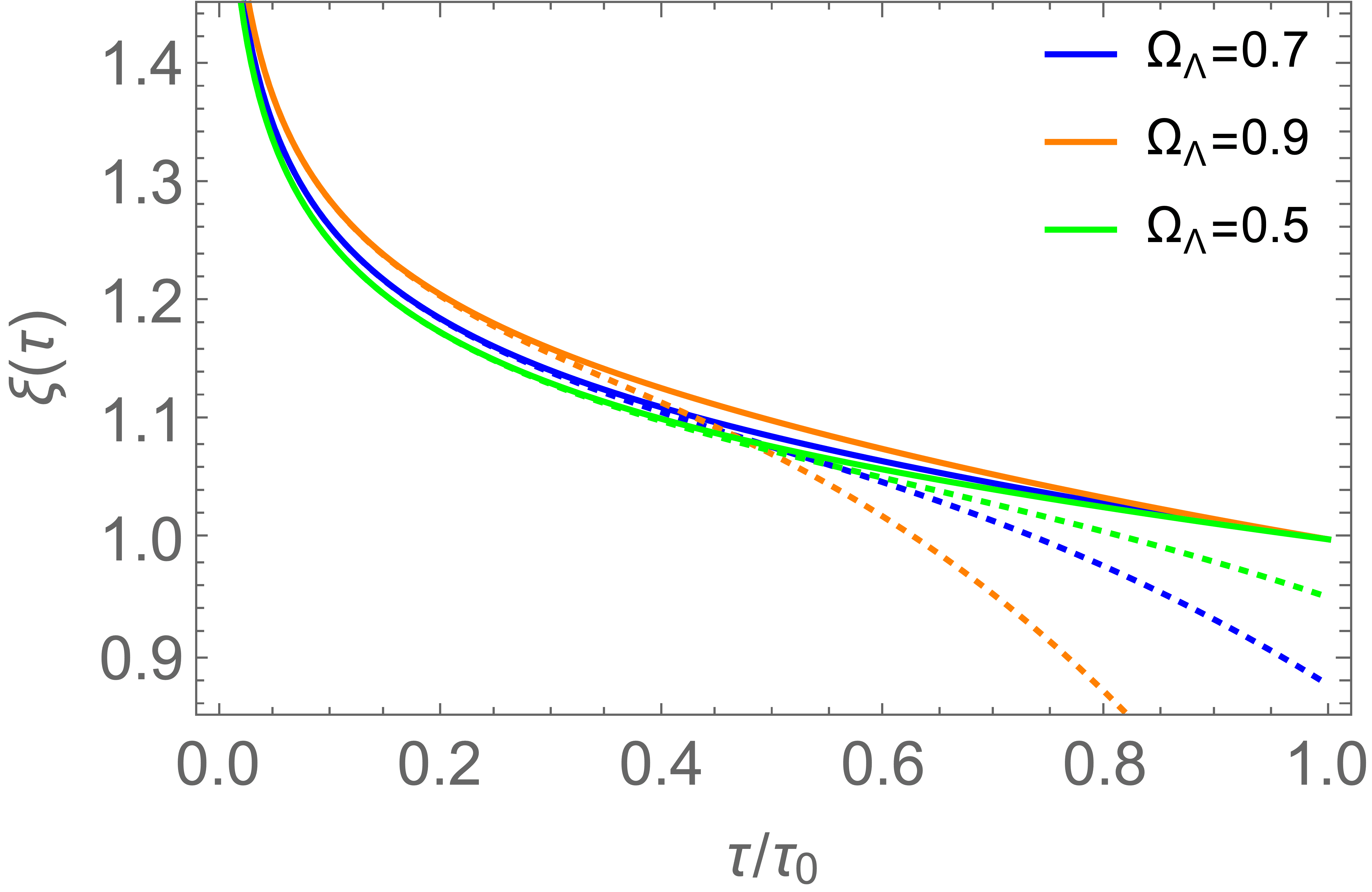
The behaviour of $a(\tau)$ and $\phi(\tau)$ have been well studied in the literature on these theories⁸⁸ 8 During dust domination the attractor solution is $a(\tau)\propto\tau^{\frac{2(1+\omega)}{2+\omega}}$ and $\phi(\tau)\propto\tau^{\frac{2}{2+\omega}}$ [32]., and we will not present them here beyond commenting that $\phi$ increases with time for positive values of $\omega$. Once these solutions are known, however, they can be used to derive values for the PPNC parameters specified in Eqs. (2.26)-(2.28). In turn, these can be used to derive the values of the parameters specified in Eqs. (2.9)-(2.12). We plot the large and small-scale values of $\mu(\tau)$ and $\xi(\tau)$ in Figures 2 and 2, for several different choices of $\omega$ and $\Omega_{\Lambda}$. The reader will note that the small-scale values of these two quantities (i.e. the solid lines) correspond directly to the values of the PPN parameters $\gamma$ and $\alpha$ at different times in cosmic history. We consider how such time dependence could be fitted in Appendix A.

In both Figures 2 and 2 we can see that at early times the behaviour of $\mu$ and $\xi$ is very similar on both large and small spatial scales. This is because the $\gamma$ and $\alpha$ terms dominate the expressions for these quantities on large scales. In fact, it is only in the presence of a non-zero $\Lambda$ that the large and small-scale limits are different. This appears to be a feature of the particular theories we are considering, and is not expected to be a generic property of theories of gravity in general. The curves that depict the small-scale limit of $\xi$ in Figure 2 can be seen to converge at $\tau=\tau_{0}$ (today), which is due to our choice of boundary condition on $\phi$. This also explains why the solid curves in the right-hand plot in Figure 2 converge today; as the value of $\gamma$ depends only on $\omega$, once $\phi_{0}$ has been fixed.

Going back in time, $\alpha$ and $\gamma$ increase for all of our theories. The differences between small and large scales, however, increase into the future. Increasing the value of $\Omega_{\Lambda}$ can be seen to exacerbate this situation, while increasing $\omega$ has the opposite effect. In general, larger values of $\omega$ can be seen to result in a slower evolution in the values of $\mu$ and $\xi$, as expected (as this is the limit in which GR is recovered). While $\alpha$ is always greater than the GR value of unity, it can be seen that $\gamma$ crosses the GR value of unity during its evolution (starting above it and finishing below it, in the cases we consider). It will be the behaviour between the large and small-scale limits depicted in these plots that will concern us for much of the rest of this study. For this we will also need to understand the evolution of perturbations.

In this section we will evolve the perturbations in our example theories, and use them to determine the scale dependence of the couplings that appear in the PPNC parameterisation. This will help to provide guidance of how the interpolation between different spatial scales works within a mathematically well-defined alternative to GR.

Let us now examine the performance of the interpolation function from Eq. (3.9), in reproducing the coupling functions from our set of example theories. For this, we will use as a specific example theory given by $\omega=10$ and $\Omega_{\Lambda}=0.7$ (i.e. the common case in Figs. 7 and 8). We specify the fractional difference between the simple interpolating function and the true value for this theory using the notation

$$\delta f=\left|\frac{f_{\text{true}}-f_{\text{interp}}}{f_{\text{true}}}\right|\,\text{,}$$

(3.11)

where $f$ here is being used to denote any one of the gravitational couplings (i.e. $\mu$, $\xi$ or $\mathcal{G}$). Figure 9 shows the accuracy of the interpolation as a function of time and scale for $\mu$ and $\xi$, as quantified by this fractional error. The range of times being shown in this figure extends from deep in the matter-dominated era through to late times in the $\Lambda$-dominated era. In creating these plots we have interpolated between gridpoints, avoiding points where our solver produced large numerical errors.

It can be seen from Figure 9 that the simple interpolation works well for both $\mu$ and $\xi$ on most spatial scales (with errors below $\sim 1\%$), but with the oscillations around the Hubble scale leading to larger errors (up to $\sim 5\%$). The detail of these plots shows some interesting structure, if we look at how the error evolves with time in each of the two cases. For the coupling $\mu$ the situation is relatively simple: there is primarily a single peak that does not change substantially with time, and which tracks the position of the Hubble scale. The coupling $\xi$ is more complicated: in this case there are several peaks that move position relative to the Hubble scale. In a cosmology with $\Lambda=0$ this more complicated behaviour does not occur, and one recovers a plot that is qualitatively similar to the case involving $\mu$.

Calculating the density contrast at $\tau_{0}$ using the parameterised equations, and the method described above, leads to results that are in good agreement with the results we obtain directly from our example theories across a range of spatial scales. There are, however, errors introduced due to the inadequacy of the simple interpolating function (3.9) to model all of the detail around the horizon scale (as was found in section 3.3). The accuracy of using the simple interpolation is displayed in the plots in Figures 11, where we show the ratio of the density contrast computed by evolving the parameterised equations with the simple interpolation to the value obtained from our example theories directly. The inaccuracy of the interpolation can be seen to create an error of order $\sim 1\%$ around the horizon scale. Decreasing $\omega$ (and therefore increasing the deviation from GR) increases this error, whereas it appears to be mostly insensitive to the value of $\Omega_{\Lambda}$. These errors are smaller than those in $\mu$ and $\xi$, as displayed in Figure 9.

As well as considering the fractional error introduced from evolving the parameterised equations with the simple interpolation, it is also of interest to consider the relative size of this error compared to the difference in density contrast that occurs due to changing the underlying theory of gravity (which is, after all, the signal that we would ultimately hope to detect). These two things are displayed at $\tau_{0}$, and over a range of spatial scales, in the left-hand plot of Figure 11. Here we have chosen to plot the fractional error in $\delta\rho$ for an example theory with $\omega=10$ and $\Omega_{\Lambda}=0.7$ (the blue curve in each of the panels in Figure 11), with the change in density contrast that one gets from increasing the value of $\omega$ to $100$ and $10^{6}$ (keeping $\Omega_{\Lambda}=0.7$ for all curves). It can be seen that the effects from changing the value of $\omega$ is much larger than the error introduced from the imperfect interpolating function, suggesting that the bias on constraints on the parameters will be small compared to any detected deviation from General Relativity. Of course this bias should still be understood or modelled, which would presumably be at the expense of adding further parameters to the framework.

In the right-hand plot of Figure 11, we compare the inaccuracies introduced from evolving the simple parameterised equations with the inaccuracies induced by applying the modified gravity parameterisation to either the background only or the perturbations only (instead of both). The inaccuracy introduced by only modifying the background or the perturbations is much larger than that introduced by evolving the simple parameterised equations directly (this is true even for theories that are much closer to GR). Interestingly, the inaccuracy introduced by not including the correct background expansion appears to be even larger than that from not evolving the perturbations with the correct equations. This result is significant for the PPNC approach because the PPNC approach provides a way to consistently parameterise both the background and the perturbations in terms of the same underlying parameters. This is not true of any other attempts at creating a theory-independent framework for testing gravity in cosmology of which we are aware. These results suggest that when constraining modified gravity in a model independent or phenomenological way, the background should generally be allowed to deviate from $\Lambda$CDM (for example using a dark energy equation of state $w(a)$) in order to prevent biasing the constraints.

We now wish to consider the effect of evolving the perturbations using the simple parameterised equations on some cosmological observables. This is not intended to be a detailed observability study, nor is it carried out in detail for specific experimental setups. Instead we wish to make a preliminary examination of how well the parameterised equations fare (in comparison to the “true” values), when calculating observables. For the lensing of light we simply have to integrate $(\Phi+\Psi)^{2}$ over the comoving distance $\chi$, from $\chi=0$ out to some source $\chi_{*}$. Doing this, we see that the parameterised equations reproduce the numerical values that one would get using the specific equations of any of our example theories with errors that are entirely negligible. This is expected, as lensing is primarily operating well within the horizon, and within this regime the parameterised equations give very good results. We also note that we reproduce the same results if we include the lensing function $\left(1-{\chi}/{\chi_{*}}\right)/\chi^{4}$ in the integral over $\chi$. This simple approach to weak-lensing calculations will of course break down on the largest angular scales; we leave a detailed examination of the effect of using the parameterised equations in this regime for future work.

As the Integrated Sachs-Wolfe (ISW) effect primarily operates over larger scales, we expect that this observable will be more sensitive to the inaccuracy of our simple interpolation between small and large scales. To investigate this, for a given $\ell$, we look at the integral giving the contribution of each $k$-mode to that $\ell$ mode:

$${\rm ISW}_{l}=\int^{\chi_{\text{max}}}_{0}d\chi\left(j_{l}\left(\dot{\Psi}+\dot{\Phi}\right)\right)^{2}\text{,}$$

(4.1)

where $j_{l}$ is the Bessel function. We calculated this quantity with both the simple parameterised equations as well as with the correct evolution for specific example theories at $\ell=10$ and $\ell=100$. Our results are shown in the left-hand panel of Figure 12. As expected, there is a noticeable difference between the curves for some $k$ values.

We can also integrate our results over $k$, with the usual factor of $k^{-1}$ to account for a scale-invariant primordial spectrum, in order to examine the accuracy of the ISW $C_{\ell}$s. This is shown by the blue curve in the right-hand plot of Figure 12. The error peaks around a couple of percent, similar to (but a little worse than) the inaccuracy we found in the density contrast. We note that these errors are never greater than $20\%$ of cosmic variance over this range of $\ell$. Finally, we again consider the consequence of changing $\omega$, and show the results in Figure 12. Again, each curve is plotted as a ratio of the results obtained in a theory with $\omega=10$, and again we see that the errors introduced by integrating the simple parameterised equations directly is substantially smaller than the change in the observable due to changing the value of $\omega$. This indicates that the errors introduced when integrating the simple parameterised equations directly is not likely to strongly bias any parameter constraints based on this observable.

References

- [1] C. M. Will. Theory and Experiment in Gravitational Physics. Cambridge University Press, 1993.
- [2] E. Poisson and C. M. Will. Gravity: Newtonian, Post-Newtonian, Relativistic. Cambridge University Press, 2014.
- [3] N. Wex. Testing relativistic gravity with radio pulsars. 2 2014.
- [4] B. P. Abbott et al. Tests of general relativity with GW150914. Phys. Rev. Lett., 116:221101, 2016.
- [5] T. Clifton, P. G. Ferreira, A. Padilla, and C. Skordis. Modified gravity and cosmology. Physics Reports, 513:1, 2012.
- [6] M. Ishak. Testing general relativity in cosmology. Living Reviews in Relativity, 22:1, 2018.
- [7] C. M. Will. The confrontation between general relativity and experiment. Living Reviews in Relativity, 17:4, 2014.
- [8] J. Gleyzes. Parametrizing modified gravity for cosmological surveys. Phys. Rev. D, 96:063516, 2017.
- [9] M. Martinelli and S. Casas. Cosmological tests of gravity: a future perspective. Universe, 7:506, 2021.
- [10] D. B. Thomas. Cosmological gravity on all scales: simple equations, required conditions, and a framework for modified gravity. Phys. Rev. D, 101:123517, 2020.
- [11] S. Srinivasan, D. B. Thomas, F. Pace, and R. Battye. Cosmological gravity on all scales. Part II. Model independent modified gravity N-body simulations. JCAP, 06:016, 2021.
- [12] F. Hassani and L. Lombriser. -body simulations for parametrized modified gravity. Mon. Not. Roy. Astron. Soc., 497:1885, 2020.
- [13] V. A. A. Sanghai and T. Clifton. Post-Newtonian cosmological modelling. Physical Review D, 91:103532, 2015.
- [14] V. A. A. Sanghai and T. Clifton. Cosmological backreaction in the presence of radiation and a cosmological constant. Phys. Rev. D, 94:023505, 2016.
- [15] T. Clifton and V. A. A. Sanghai. Parametrizing theories of gravity on large and small scales in cosmology. Phys. Rev. Lett., 122:011301, 2019.
- [16] T. Anton and T. Clifton. The momentum constraint equation in parameterised post-Newtonian cosmology. Class. Quant. Grav., 39:095005, 2021.
- [17] T. Clifton, C. S. Gallagher, S. Goldberg, and K. A. Malik. Viable gauge choices in cosmologies with nonlinear structures. Phys. Rev. D, 101:063530, 2020.
- [18] B. Bertotti, L. Iess, and P. Tortora. A test of general relativity using radio links with the Cassini spacecraft. Nature, 425:374, 2003.
- [19] R. Caldwell, A. Cooray, and A. Melchiorri. Constraints on a new post-general relativity cosmological parameter. Physical Review D, 76:023507, 2007.
- [20] L. Amendola, M. Kunz, and D. Sapone. Measuring the dark side (with weak lensing). Journal of Cosmology and Astroparticle Physics, 2008:013, 2008.
- [21] S. R. Goldberg, T. Clifton, and K. A. Malik. Cosmology on all scales: a two-parameter perturbation expansion. Phys. Rev. D, 95:043503, 2017.
- [22] G. Gubitosi, F. Piazza and F. Vernizzi. The Effective Field Theory of Dark Energy. JCAP, 02:032, 2013.
- [23] E. Bellini and I. Sawicki. Dark energy or modified gravity? An effective field theory approach. JCAP, 08:010, 2013.
- [24] J. K. Bloomfield, E. E. Flanagan, M. Park and S. Watson. Maximal freedom at minimum cost: linear large-scale structure in general modifications of gravity. JCAP, 07:050, 2014.
- [25] S. Tassev, M. Zaldarriaga and D. Eisenstein. Solving Large Scale Structure in Ten Easy Steps with COLA JCAP, 06:036, 2013.
- [26] P. G. Bergmann. Comments on the scalar-tensor theory. International Journal of Theoretical Physics, 1:25, 1968.
- [27] R. V. Wagoner. Scalar-tensor theory and gravitational waves. Physical Review D, 1:3209, 1970.
- [28] C. Brans and R. H. Dicke. Mach’s principle and a relativistic theory of gravitation. Phys. Rev., 124:925, 1961.
- [29] G. W. Horndeski. Second-order scalar-tensor field equations in a four-dimensional space. International Journal of Theoretical Physics, 10:363, 1974.
- [30] J.-P. Uzan. Varying constants, gravitation and cosmology. Living reviews in relativity, 14:1, 2011.
- [31] V. A. A. Sanghai and T. Clifton. Parameterized post-Newtonian cosmology. Classical and Quantum Gravity, 34:065003, 2017.
- [32] H. Nariai. On the Green’s function in an expanding universe and its role in the problem of Mach’s principle. Progress of Theoretical Physics, 40:49, 1968.
- [33] K. A. Malik and D. Wands. Cosmological perturbations. Physics Reports, 475:1, 2009.
- [34] C. Gordon, D. Wands, B. A. Bassett, and R. Maartens. Adiabatic and entropy perturbations from inflation. Physical Review D, 63:023506, 2000.
- [35] M. A. Amin, R. V. Wagoner, and R. D. Blandford. A subhorizon framework for probing the relationship between the cosmological matter distribution and metric perturbations. Monthly Notices of the Royal Astronomical Society, 390:131, 2008.
- [36] T. Baker and P. Bull. Observational signatures of modified gravity on ultra-large scales. Astrophys. J., 811:116, 2015.
- [37] G. Brando et al. Fully relativistic predictions in Horndeski gravity from standard Newtonian N-body simulations. JCAP, 09:024, 2021.
- [38] M. Bruni, D. B. Thomas and D. Wands. Computing General Relativistic effects from Newtonian N-body simulations: frame dragging in the post-Friedmann approach. Physical Review D, 89:044010, 2014.
- [39] D. B. Thomas, M. Bruni and D. Wands. Relativistic weak lensing from a fully non-linear cosmological density field. JCAP, 09:021, 2015.
- [40] D. B. Thomas, M. Bruni and D. Wands. The fully non-linear post-Friedmann frame-dragging vector potential: magnitude and time evolution from N-body simulations. Monthly Notices of the Royal Astronomical Society, 452:1727, 2015.
- [41] D. B. Thomas et al. f(R) gravity on non-linear scales: the post-Friedmann expansion and the vector potential. JCAP, 07:051, 2015.
- [42] J. Adamek, D. Daverio, R. Durrer, and M. Kunz. General Relativistic N-body simulations in the weak field limit. Physical Review D, 88:103527, 2013.
- [43] J. Adamek, R. Durrer, and M. Kunz. N-body methods for relativistic cosmology. Classical and Quantum Gravity, 31:234006, 2014.
- [44] J. Adamek, D. Daverio, R. Durrer, and M. Kunz. Gevolution: a cosmological N-body code based on general relativity. JCAP, 07:053, 2016.