We consider the scotogenic model introducing three right-handed neutrinos $N_{i}~(i=1,2,3)$ with the mass $m_{i}$ and an inert doublet scalar $\eta$ with hypercharge $+1/2$ to the SM [18]. The $\mathbb{Z}_{2}$ parity is also imposed on the model such that the new particles are odd, whereas all the SM particles are even. The Lagrangian for the neutrino Yukawa coupling is given by

$\displaystyle\mathcal{L}_{Y}=-y_{i\alpha}\eta\overline{N_{i}}P_{L}L_{\alpha}+\mathrm{h.c.},$

(2.1)

where $L_{\alpha}=(\nu_{\alpha},\ell_{\alpha}^{-})^{T}$ is the SM lepton doublets with the flavor index $\alpha=e,\mu,\tau$. The scalar potential invariant under the symmetry is given by

	$\displaystyle V_{0}=$	$\displaystyle~\mu_{\Phi}^{2}|\Phi|^{2}+\mu_{\eta}^{2}|\eta|^{2}+\lambda_{1}|\Phi|^{4}+\lambda_{2}|\eta|^{4}$
		$\displaystyle+\lambda_{3}|\Phi|^{2}|\eta|^{2}+\lambda_{4}|\eta^{{\dagger}}\Phi|^{2}+\frac{\lambda_{5}}{2}\left[\left(\eta^{\dagger}\Phi\right)^{2}+\mathrm{h.c.}\right].$		(2.2)

The scalar fields $\Phi$ and $\eta$ are parametrized as³³ 3 It is known that the existence of the neutral CP-conserving vacuum indicates there are no deeper charge-breaking or CP-violating vacua at tree-level [31]. Hence, we do not consider such CP-violating vacua.

$\displaystyle\Phi=\frac{1}{\sqrt{2}}\left(\begin{array}[]{c}w^{+}\\ \phi_{1}+h+iz\end{array}\right),\qquad\eta=\left(\begin{array}[]{c}\eta^{+}\\ (\phi_{2}+H+iA)/\sqrt{2}\end{array}\right),$

where $w^{+}$ and $z$ are the Nambu-Goldstone bosons absorbed by the $W$ boson and the $Z$ boson after the EW symmetry breaking. Note that only the neutral CP-even scalar field in $\Phi$ obtains the vacuum expectation value (VEV) at zero temperature, namely $\phi_{1}(T=0)\equiv v=246$ GeV.

The squared masses of the physical scalar particles at zero temperature are given by

	$\displaystyle m_{h}^{2}$	$\displaystyle=2\lambda_{1}v^{2},$		(2.7)
	$\displaystyle m_{\eta^{\pm}}^{2}$	$\displaystyle=\mu_{\eta}^{2}+\frac{\lambda_{3}}{2}v^{2},$		(2.8)
	$\displaystyle m_{H}^{2}$	$\displaystyle=\mu_{\eta}^{2}+\frac{\lambda_{3}+\lambda_{4}+\lambda_{5}}{2}v^{2},$		(2.9)
	$\displaystyle m_{A}^{2}$	$\displaystyle=\mu_{\eta}^{2}+\frac{\lambda_{3}+\lambda_{4}-\lambda_{5}}{2}v^{2},$		(2.10)

where the stationary condition $\mu_{\Phi}^{2}=-\lambda_{1}v^{2}$ is used, and $h$ corresponds to the SM Higgs boson, with the mass $m_{h}=125~\mathrm{GeV}$. From above equations, we can get

	$\displaystyle\lambda_{3}$	$\displaystyle=\frac{2}{v^{2}}(m_{\eta^{\pm}}^{2}-\mu_{\eta}^{2}),$		(2.11)
	$\displaystyle\lambda_{4}$	$\displaystyle=\frac{m_{H}^{2}+m_{A}^{2}-2m_{\eta^{\pm}}^{2}}{v^{2}},$		(2.12)
	$\displaystyle\lambda_{5}$	$\displaystyle=\frac{m_{H}^{2}-m_{A}^{2}}{v^{2}}.$		(2.13)

We take the masses of the inert scalar particles, $m_{\eta^{\pm}},m_{H}$, and $m_{A}$, as input parameters instead of $\lambda_{3},\lambda_{4},$ and $\lambda_{5}$ in the scalar potential of Eq. (2.2). The other parameters $\mu_{\eta}^{2}$ and $\lambda_{2}$ remain as free parameters.

In this model, the neutrino masses are generated at the one-loop level, and the mass formula is given by

$\displaystyle(m_{\nu})_{\alpha\beta}=\sum_{i=1}^{3}\frac{y_{i\alpha}y_{i\beta}m_{i}}{2(4\pi)^{2}}\left[\frac{m_{H}^{2}}{m_{H}^{2}-m_{i}^{2}}\log\left(\frac{m_{H}^{2}}{m_{i}^{2}}\right)-\frac{m_{A}^{2}}{m_{A}^{2}-m_{i}^{2}}\log\left(\frac{m_{A}^{2}}{m_{i}^{2}}\right)\right]\equiv\left(y^{T}\Lambda y\right)_{\alpha\beta}.$

(2.14)

This mass matrix can be diagonalized by the Pontecorvo-Maki-Nakagawa-Sakata (PMNS) matrix $U_{\mathrm{PMNS}}$ as $U_{\mathrm{PMNS}}^{T}m_{\nu}U_{\mathrm{PMNS}}=\hat{m}_{\nu}$ where $\hat{m}_{\nu}$ is the diagonalized neutrino mass matrix. The Yukawa matrix is given by the Casas-Ibarra parametrization [32]

$\displaystyle y=\sqrt{\Lambda}^{-1}C\sqrt{\hat{m}_{\nu}}U_{\mathrm{PMNS}}^{{\dagger}},$

(2.15)

where $C$ is a complex orthogonal matrix satisfying $C^{T}C=CC^{T}=\mbox{1}\hskip-2.5pt\mbox{l}_{3\times 3}$. The neutrino mass eigenvalues and mixing angles consistent with the neutrino oscillation data can be reproduced as long as we choose this parametrization. In the following, we assume that the second and third right-handed neutrinos ($N_{2}$ and $N_{3}$) are much heavier than the first right-handed neutrino $N_{1}$ and the inert scalar particles. This assumption indicates that the neutrino Yukawa couplings naturally have the hierarchy $|y_{1\alpha}|\ll|y_{2\alpha}|,|y_{3\alpha}|$ via Eq. (2.15). Thus such hierarchical Yukawa couplings lead to fast decays of the heavier right-handed neutrinos into the lightest one, and we do not need to consider the effect of these particles on the dark matter relic abundance as will be seen later.

We consider the theoretical constraints as follows. First, the conditions for the tree level potential bounded from below are given by

$\displaystyle\lambda_{1}>0,~~\lambda_{2}>0,~~-2\sqrt{\lambda_{1}\lambda_{2}}<\lambda_{3},~~-2\sqrt{\lambda_{1}\lambda_{2}}<\lambda_{3}+\lambda_{4}-\lambda_{5},$

(2.16)

and the perturbativity conditions are given by

$\displaystyle|\lambda_{n}|<4\pi\ (n=1,2,\cdots 5).$

(2.17)

In addition to the above perturbative conditions, we consider the tree-level unitarity bound [33, 34, 35]. Furthermore, we impose the condition that the EW vacuum is absolutely stable, namely it should not be metastable with a lifetime long enough compared to the age of the universe [31, 36]. We numerically check that the EW vacuum is the global minimum in the region for $|\phi_{i}|\leq 10$ TeV in the later part of the paper.

For the experimental constraints, the LEP precisely measured the decay widths of the $W$ and $Z$ bosons [37] and does not allow a window for new decay channels into the inert scalar particles. Namely, the masses should satisfy

$$m_{H}+m_{\eta^{\pm}}>m_{W},~~m_{A}+m_{\eta^{\pm}}>m_{W},~~m_{H}+m_{A}>m_{Z},~~2m_{\eta^{\pm}}>m_{Z}.$$

(2.18)

Additionally neutral final states searches at the LEP [38] exclude the mass region

$$m_{H}<80~\mathrm{GeV}~\cap~m_{A}<100~\mathrm{GeV}~\cap~m_{A}-m_{H}>8~\mathrm{GeV}.$$

(2.19)

There is the lower bound for the charged inert scalar

$$m_{\eta^{\pm}}>70~\mathrm{GeV}.$$

(2.20)

This bound comes from the charged scalar pair production searches at LEP [39]. We also consider the constraints from the EW precision data, which can be avoided by assuming the mass degeneracy between the charged and neutral inert scalars ($m_{\eta^{\pm}}\approx m_{H}$ or $m_{A}$), because the custodial symmetry recovers in this limit [40]. Note that the neutral inert scalars do not contribute to the Higgs boson invisible decay because we set the neutral inert scalar masses such that any combination of those is smaller than the SM Higgs boson mass.

The finite temperature effective potential at the one-loop $V^{T}$ is given by

$\displaystyle V^{T}=V_{0}+V_{\rm CW}+V_{\rm CT}+V_{1}^{T},$

(3.1)

where $V_{0}$ is the potential at the tree-level given by Eq. (2.2), $V_{\rm CW}$ is the one-loop Coleman-Weinberg potential [41], $V_{\rm CT}$ is the counterterm potential, and $V_{1}^{T}$ is the one-loop effective potential at finite temperature [42], respectively.

The Coleman Weinberg potential can be written as [41]

$\displaystyle V_{\rm CW}(\phi_{1},\phi_{2})=\pm\frac{1}{64\pi^{2}}\sum_{k}n_{k}m_{k}^{4}(\phi_{1},\phi_{2})\left[\log\frac{m_{k}^{2}(\phi_{1},\phi_{2})}{\mu^{2}}-C_{k}\right],$

(3.2)

where the index $k$ denotes particle species, $m_{k}$ and $n_{k}$ are the mass and degrees of freedom of a particle $k$. Specifically, the degrees of freedom are given by $n_{k}=2,1,1,1,6,3,2,12,12$, and 4 for $k=\eta^{\pm},h,H,A,W,Z,\gamma,t,b$, and $\tau$, respectively. Note that we include only the contributions from top and bottom quarks, and tau as fermions because the other contributions are negligible due to its small Yukawa couplings. The overall plus sign in Eq. (3.2) is for the boson contributions, while the minus sign is for the fermion contributions. The renormalization scale denoted by $\mu$ is fixed to be $\mu=v$. Because we choose the $\overline{{\rm MS}}$ scheme for the renormalization, the coefficients $C_{k}$ are $1/2$ for the transverse gauge bosons but $3/2$ for the other particle species. In general, the quantum corrections shift the position of the EW vacuum and the masses of the scalar fields from the original ones. The counterterm $V_{\rm CT}$ is determined, such that these quantities are fixed at the tree-level,

	$\displaystyle\left.\frac{\partial V_{\rm CT}(\phi_{1},\phi_{2})}{\partial\phi_{i}}\right|_{(\phi_{1},\phi_{2})=(v,0)}$	$\displaystyle=-\left.\frac{\partial V_{\rm CW}(\phi_{1},\phi_{2})}{\partial\phi_{i}}\right|_{(\phi_{1},\phi_{2})=(v,0)}\equiv-V_{i},$		(3.3)
	$\displaystyle\left.\frac{\partial^{2}V_{\rm CT}(\phi_{1},\phi_{2})}{\partial\phi_{i}\partial\phi_{j}}\right|_{(\phi_{1},\phi_{2})=(v,0)}$	$\displaystyle=-\left.\frac{\partial^{2}V_{\rm CW}(\phi_{1},\phi_{2})}{\partial\phi_{i}\partial\phi_{j}}\right|_{(\phi_{1},\phi_{2})=(v,0)}\equiv-V_{ij}\ \ (i,j=1,2).$		(3.4)

We set $V_{\rm CT}$ following Ref. [14], as

$\displaystyle V_{\rm CT}=\delta\mu_{\Phi}^{2}\phi_{1}^{2}+\delta\mu_{\eta}^{2}\phi_{2}^{2}+\delta\lambda_{1}\phi_{1}^{4},$

(3.5)

with

		$\displaystyle\delta\mu_{\Phi}^{2}=-\frac{3}{4v}V_{1}+\frac{1}{4}V_{11},$		(3.6)
		$\displaystyle\delta\mu_{\eta}^{2}=-\frac{1}{2}V_{22},$
		$\displaystyle\delta\lambda_{1}=\frac{1}{8v^{3}}(V_{1}-vV_{11}).$

When calculating the coefficients $\delta\mu_{\Phi}^{2},\delta\mu_{\eta}^{2}$, and $\delta\lambda_{1}$ numerically, infrared log divergences arise in the second derivatives of $V_{\rm CW}$ for the Nambu-Goldstone boson contributions. These divergences are removed by introducing a cut-off for the Nambu-Goldstone boson masses. Here we take the cut-off at $m_{h}$ [43].

The one-loop effective potential at finite temperature is given by [42]

$\displaystyle V_{1}^{T}(\phi_{1},\phi_{2})=\pm\frac{T^{4}}{2\pi^{2}}\sum_{k}\int_{0}^{\infty}dx\ x^{2}\ln\left[1\mp\exp\left(-\sqrt{x^{2}+\frac{m_{k}^{2}(\phi_{1},\phi_{2})}{T^{2}}}\right)\right],$

(3.7)

with the temperature $T$. The upper (lower) sign is for bosonic (fermionic) contributions.

We take into account the corrections from the ring (Sazae-san) diagrams to avoid infrared divergences arising in loop expansions [44, 45]. For this purpose, we apply the Parwani resummation method [44], which is suitable for evaluating multi-step PTs because this method does not contain the high-temperature expansion [15].⁴⁴ 4 The state-of-the-art computations of the effective potential including higher order terms of perturbation have been studied in Refs. [46, 47, 48, 49]. We can perform this method by inserting masses with thermal corrections to $m_{k}^{2}$ in $V_{1}^{T}$. The thermal masses used for this method are described in the following subsection.

The inert scalar field $\eta$ may temporarily have a VEV at finite temperature. Then, it should vanish at zero temperature not to spontaneously break the $\mathbb{Z}_{2}$ parity. Thus, the mass matrices for the inert scalar particles at finite temperature can have a different shape from those at zero temperature. The mass matrices for the charged scalars $(w^{+},\eta^{+})$, the CP-even scalars $(h,H)$ and the CP-odd scalars $(z,A)$ are field-dependent and given by

	$\displaystyle\mathcal{M}_{\rm charge}^{2}=$	$\displaystyle~\frac{1}{2}\left(\begin{array}[]{cc}2\mu_{\Phi}^{2}+2\lambda_{1}\phi_{1}^{2}+\lambda_{3}\phi_{2}^{2}+c_{1}T^{2}&(\lambda_{4}+\lambda_{5})\phi_{1}\phi_{2}\\ (\lambda_{4}+\lambda_{5})\phi_{1}\phi_{2}&2\mu_{\eta}^{2}+2\lambda_{2}\phi_{2}^{2}+\lambda_{3}\phi_{1}^{2}+c_{2}T^{2}\end{array}\right),$
	$\displaystyle\mathcal{M}_{\rm odd}^{2}=$	$\displaystyle~\frac{1}{2}\left(\begin{array}[]{cc}2\mu_{\Phi}^{2}+2\lambda_{1}\phi_{1}^{2}+\overline{\lambda}_{345}\phi_{2}^{2}+c_{1}T^{2}&2\lambda_{5}\phi_{1}\phi_{2}\\ 2\lambda_{5}\phi_{1}\phi_{2}&2\mu_{\eta}^{2}+2\lambda_{2}\phi_{2}^{2}+\overline{\lambda}_{345}\phi_{1}^{2}+c_{2}T^{2}\end{array}\right),$
	$\displaystyle\mathcal{M}_{\rm even}^{2}=$	$\displaystyle~\frac{1}{2}\left(\begin{array}[]{cc}2\mu_{\Phi}^{2}+6\lambda_{1}\phi_{1}^{2}+\lambda_{345}\phi_{2}^{2}+c_{1}T^{2}&2\lambda_{345}\phi_{1}\phi_{2}\\ 2\lambda_{345}\phi_{1}\phi_{2}&2\mu_{\eta}^{2}+6\lambda_{2}\phi_{2}^{2}+\lambda_{345}\phi_{1}^{2}+c_{2}T^{2}\end{array}\right),$

where the coupling $\overline{\lambda}_{345}$ is defined as $\overline{\lambda}_{345}\equiv\lambda_{3}+\lambda_{4}-\lambda_{5}$, and the coefficients $c_{1}$ and $c_{2}$ are given by

		$\displaystyle c_{1}=\frac{1}{8}g^{2}+\frac{1}{16}(g^{2}+g^{\prime 2})+\frac{1}{2}\lambda_{1}+\frac{1}{6}\lambda_{3}+\frac{1}{12}\lambda_{4},$		(3.14)
		$\displaystyle c_{2}=\frac{1}{8}g^{2}+\frac{1}{16}(g^{2}+g^{\prime 2})+\frac{1}{2}\lambda_{2}+\frac{1}{6}\lambda_{3}+\frac{1}{12}\lambda_{4}+\frac{1}{4}y_{t}^{2}+\frac{1}{4}y_{b}^{2}+\frac{1}{12}y_{\tau}^{2},$		(3.15)

with the $SU(2)_{L}$ and $U(1)_{Y}$ gauge couplings $g$ and $g^{\prime}$, and the Yukawa couplings $y_{t},y_{b}$ and $y_{\tau}$ for top, bottom, and tau, respectively. We regard the mass eigenvalues obtained by diagonalizing the above mass matrices as the physical masses with thermal effects.

The gauge bosons also get thermal corrections. In fact, only the longitudinal modes get thermal corrections, whereas the transverse modes do not. The masses for the transverse modes of the $W$ boson, $Z$ boson, and photon are written as

	$\displaystyle m_{W_{T}}^{2}=$	$\displaystyle~\frac{g^{2}}{4}(\phi_{1}^{2}+\phi_{2}^{2}),$		(3.16)
	$\displaystyle m_{Z_{T}}^{2}=$	$\displaystyle~\frac{1}{4}(g^{2}+g^{\prime 2})(\phi_{1}^{2}+\phi_{2}^{2}),$		(3.17)
	$\displaystyle m_{\gamma_{T}}^{2}=$	$\displaystyle~0.$		(3.18)

On the other hand, the $W$ boson mass for the longitudinal mode with thermal corrections is given by [50]

$$m_{W_{L}}^{2}=\frac{g^{2}}{4}(\phi_{1}^{2}+\phi_{2}^{2})+2g^{2}T^{2}.$$

(3.19)

For the longitudinal $Z$ boson and photon, the masses are obtained by diagonalizing the following mass matrix

$\displaystyle\frac{1}{4}(\phi_{1}^{2}+\phi_{2}^{2})\left(\begin{array}[]{cc}g^{2}&-gg^{\prime}\\ -gg^{\prime}&g^{\prime 2}\\ \end{array}\right)+\left(\begin{array}[]{cc}2g^{2}T^{2}&0\\ 0&2g^{\prime 2}T^{2}\\ \end{array}\right)\,.$

Then, we obtain the mass eigenvalues as

	$\displaystyle m_{Z_{L}}^{2}=$	$\displaystyle~\frac{1}{8}(g^{2}+g^{\prime 2})(\phi_{1}^{2}+\phi_{2}^{2}+8T^{2})+\Delta,$		(3.24)
	$\displaystyle m_{\gamma_{L}}^{2}=$	$\displaystyle~\frac{1}{8}(g^{2}+g^{\prime 2})(\phi_{1}^{2}+\phi_{2}^{2}+8T^{2})-\Delta,$		(3.25)

where $\Delta$ is given by

$\displaystyle\Delta=\sqrt{\frac{1}{64}(g^{2}+g^{\prime 2})^{2}(\phi_{1}^{2}+\phi_{2}^{2}+8T^{2})^{2}-g^{2}g^{\prime 2}T^{2}(\phi_{1}^{2}+\phi_{2}^{2}+4T^{2})}.$

(3.26)

In general, various PT patterns are possible. In the following analyses, we consider only the patterns shown in Fig. 1. The one-step PT denotes the transition occurring only once from the origin $(\phi_{1},\phi_{2})=(0,0)$ to the EW vacuum $(v,0)$. Besides, the two-step PT is referred to the transition going to the EW vacuum via two steps: $(\phi_{1},\phi_{2})=(0,0)\to(0,v^{\prime})\to(v,0)$. The 2nd PT of the two-step must be first-order because the potential barrier (saddle point of the potential) exists between the two minima. There is another possibility of two-step PTs: $(\phi_{1},\phi_{2})=(0,0)\to(v^{\prime\prime},v^{\prime})\to(v,0)$. However this transition hardly occurs in the scotogenic model because the quadratic cross term $\Phi^{\dagger}\eta$ in the scalar potential is forbidden by the $\mathbb{Z}_{2}$ parity.

To reveal the impact of PTs on the dark matter relic density, we perform a parameter search using CosmoTransitions for evaluating PTs [51]. The independent parameters are randomly selected $5\times 10^{6}$ times in total from the intervals:

		$\displaystyle 70~\mathrm{GeV}<m_{\eta^{\pm}}=m_{A}\leq 1000~\mathrm{GeV},\quad 55~\mathrm{GeV}\leq m_{H}\leq 1000~\mathrm{GeV},$
		$\displaystyle 0\leq\lambda_{2}\leq 4\pi,\quad-(1000~\mathrm{GeV})^{2}\leq\mu_{\eta}^{2}\leq(1000~\mathrm{GeV})^{2},$

where the lower bound on $m_{\eta^{\pm}}$ follows Eq. (2.20). We assume that the inert scalar masses for $\eta^{\pm}$ and $A$ are degenerate $(m_{\eta^{\pm}}=m_{A})$ so that the constraint of the EW precision measurements is easily satisfied as referred to in Sec. 2.2. Tab. 1 shows the minimum and maximum values of each parameter obtained by our parameter search and the number of parameter sets (last column) calculated, considering the relevant constraints. The fourth and fifth rows with the symbol ^∗ denote the parameter sets satisfying the conditions $m_{\eta}/T_{n}>25$ and $\phi_{2}(T_{n2})/T_{n2}>1$, respectively. Here $m_{\eta}$ means the smallest mass of the inert scalar boson and the nucleation temperature $T_{n}$ is determined by the condition of one bubble nucleation per Hubble radius: $S_{3}(T_{n})/T_{n}\simeq 140$ with the $O(3)$ symmetric action $S_{3}$. For the two-step PT, we define the nucleation temperature of the first step as $T_{n1}$ and that of the second step $T_{n2}$. Note that the one-step^∗ PT is necessarily first-order because the conditions $m_{\eta}/T_{n}>25$ demands $T_{n}$ to be very low temperature.

Only the parameter sets with the symbol ^∗ can potentially influence the calculation of dark matter relic abundance. One can find that the parameter region affected by the PTs is limited. Therefore the previous studies on dark matter in the scotogenic model remain correct except for some specific parameter regions. However we emphasize that $19\%~(=333/1758)$ of two-step PTs can have an impact on the dark matter relic density, which is not small. Fig. 2 shows the distribution of the number of parameter sets as a function of $m_{\eta}/T_{n}$ for the one-step PTs and $\phi_{2}(T_{n2})/T_{n2}$ for the two-step PTs. The red vertical lines show the thresholds $m_{\eta}/T_{n}=25$ and $\phi_{2}(T_{n2})/T_{n2}=1$. The parameter sets with the symbol ^∗ in Tab. 1 correspond to results on the right side of the red line in Fig. 2.

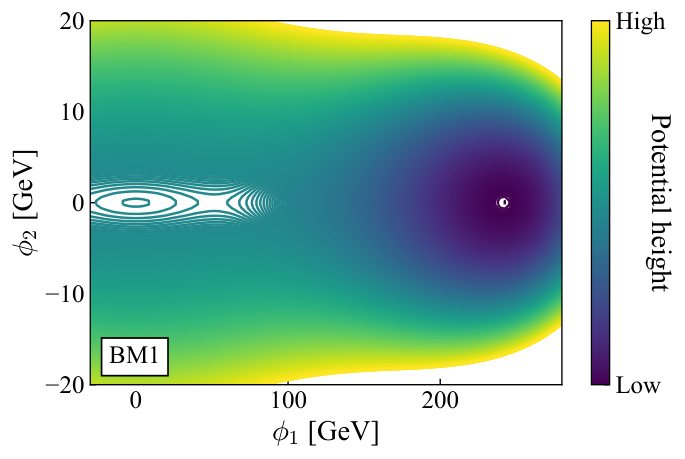
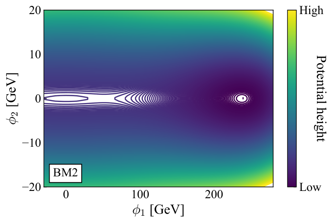
To see the impact of PTs on the dark matter relic density specifically, we choose four benchmark parameter sets in Tab. 2. All constraints in Sec. 2.2 are satisfied at the benchmark parameter sets. Fig. 3 shows the contours of the thermal effective potential at $T=T_{n}$ for BM1 and BM2 where the nucleation temperature is determined as $T_{n}=23~\mathrm{GeV}$ for BM1 and $T_{n}=25~\mathrm{GeV}$ for BM2.⁵⁵ 5 One may consider $\sqrt{\phi_{1}^{2}+\phi_{2}^{2}}/T$ at critical temperatures are too large as $10$ [52] because of such a low $T_{n}$. However, those values are not so sizable ($4$–$4.8$) for BM1 and BM2. For both benchmark parameter sets, the first-order PTs occur from the origin to the EW vacuum.

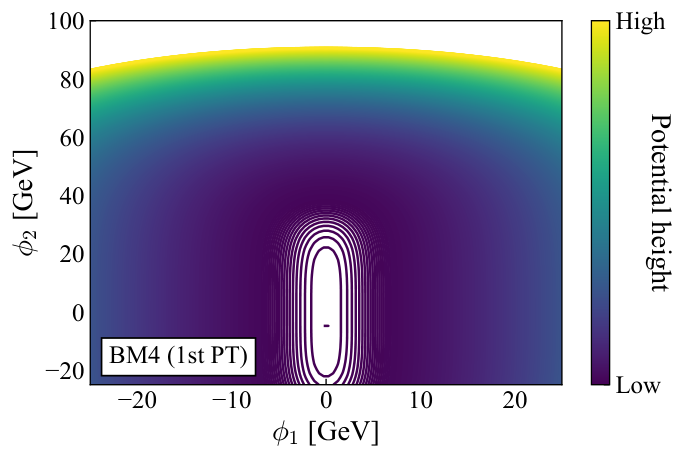
The two-step PTs occur for BM3 and BM4, unlike BM1 and BM2. Fig. 4 represents the contours of the finite temperature effective potential for BM3 (top) and BM4 (bottom) at $T=T_{n1}$ (left) and $T_{n2}$ (right) where $T_{n1}$ and $T_{n2}$ are the nucleation temperatures for the first and second step PTs, respectively.⁶⁶ 6 The nucleation temperature cannot be defined for the first PT for BM4 because the bubbles are not produced for the second-order PT. Nevertheless, we simply regard $T_{n1}$ for BM4 as the temperature where the second-order PT occurs in this paper. The nucleation temperatures for BM3 are numerically determined as $T_{n1}=148~\mathrm{GeV}$ and $T_{n2}=86~\mathrm{GeV}$ while these are $T_{n1}=184~\mathrm{GeV}$ and $T_{n2}=66~\mathrm{GeV}$ for BM4. We confirmed that the numerical determination of the nucleation temperatures with CosmoTransitions is stable enough near the BM parameter sets.

GWs are generated by the first-order PTs. The generated GW energy density is described by the two parameters $\alpha$ and $\tilde{\beta}$, which are defined by

	$\displaystyle\alpha\equiv$	$\displaystyle\left.\frac{\epsilon(T)}{\rho_{\rm rad}(T)}\right|_{T=T_{n}}\,,$		(3.27)
	$\displaystyle\tilde{\beta}\equiv$	$\displaystyle\left.\left[T\frac{d}{dT}\left(\frac{S_{3}(T)}{T}\right)\right]\right|_{T=T_{n}}\,,$		(3.28)

at the nucleation temperature $T_{n}$. The parameter $\alpha$ represents the PT strength and $\tilde{\beta}$ is equal to $\beta/H(T=T_{n})$ where $\beta$ describes the inverse time duration of the PT and $H(T=T_{n})$ is the Hubble rate at $T=T_{n}$. In the case of two-step PTs, the above two parameters are obtained at each nucleation temperature $T_{n1}$ and $T_{n2}$. In Eq. (3.27), $\epsilon(T)$ is the latent heat, and $\rho_{\rm rad}(T)$ is the radiation density given by $\rho_{\rm rad}(T)=\pi^{2}g_{*}T^{4}/30$ with the effective relativistic degrees of freedom in the symmetric phase $g_{*}$.

There are three contributions to the GW energy density, which are given by

$\displaystyle\Omega_{\text{GW}}h^{2}=\Omega_{\varphi}h^{2}+\Omega_{\text{sw}}h^{2}+\Omega_{\text{turb}}h^{2}\,,$

(3.29)

where $h$ denotes the dimensionless Hubble rate, $\Omega_{\varphi}$ is the scalar field contribution from bubble wall collisions [53, 54, 55, 56, 57, 58], $\Omega_{\rm sw}$ is the sound wave contribution surrounding the bubble walls [59, 60], and $\Omega_{\rm turb}$ is the contribution from magnetohydrodynamic turbulence in plasma [61, 62, 63, 64, 65, 66]. Numerical simulations and analytic estimation formulate each contribution to the GW energy density as follows [58, 60, 65, 66],

	$\displaystyle\Omega_{\varphi}h^{2}=$	$\displaystyle~1.67\times 10^{-5}\tilde{\beta}^{-2}\left(\frac{\kappa_{\varphi}\alpha}{1+\alpha}\right)^{2}\left(\frac{100}{g_{*}}\right)^{\frac{1}{3}}\left(\frac{0.11v^{3}_{w}}{0.42+v_{w}^{2}}\right)\frac{3.8(f/f_{\varphi})^{2.8}}{1+2.8(f/f_{\varphi})^{3.8}},$		(3.30)
	$\displaystyle\Omega_{\mathrm{sw}}h^{2}=$	$\displaystyle~2.65\times 10^{-6}\tilde{\beta}^{-1}\left(\frac{\kappa_{\text{sw}}\alpha}{1+\alpha}\right)^{2}\left(\frac{100}{g_{*}}\right)^{\frac{1}{3}}v_{w}(f/f_{\mathrm{sw}})^{3}\left(\frac{7}{4+3(f/f_{\mathrm{sw}})^{2}}\right)^{\frac{7}{2}},$		(3.31)
	$\displaystyle\Omega_{\mathrm{turb}}h^{2}=$	$\displaystyle~3.35\times 10^{-4}\tilde{\beta}^{-1}\left(\frac{\kappa_{\text{turb}}\alpha}{1+\alpha}\right)^{\frac{3}{2}}\left(\frac{100}{g_{*}}\right)^{\frac{1}{3}}v_{w}\frac{(f/f_{\mathrm{turb}})^{3}}{[1+(f/f_{\mathrm{turb}})]^{\frac{11}{3}}(1+8\pi f/h_{n})},$		(3.32)

where $v_{w}$ is the bubble wall velocity taken to be $v_{w}=1$ for simplicity. The additional parameters $\kappa_{\varphi}$, $\kappa_{\mathrm{sw}}$, and $\kappa_{\rm turb}$ are the fraction of vacuum energy converted into gradient energy of the scalar field, the bulk motion of the fluid, and magnetohydrodynamic turbulence, respectively. These are estimated as [56, 67, 60]

	$\displaystyle\kappa_{\varphi}\approx$	$\displaystyle~\frac{1}{1+0.715\alpha}\left(0.715\alpha+\frac{4}{27}\sqrt{\frac{3\alpha}{2}}\right),$		(3.33)
	$\displaystyle\kappa_{\mathrm{sw}}\approx$	$\displaystyle~\frac{\alpha}{0.73+0.083\sqrt{\alpha}+\alpha},$		(3.34)
	$\displaystyle\kappa_{\rm turb}\approx$	$\displaystyle~0.1\kappa_{\mathrm{sw}}.$		(3.35)

In Eqs. (3.30)–(3.32), $f$ is the GW frequency at present, and the peak frequencies $f_{\varphi}$, $f_{\mathrm{sw}}$ and $f_{\mathrm{turb}}$ are given by [58, 60, 65, 66]

	$\displaystyle f_{\varphi}=$	$\displaystyle~1.65\times 10^{-5}\mathrm{Hz}~\tilde{\beta}\left(\frac{0.62}{1.8-0.1v_{w}+v^{2}_{w}}\right)\left(\frac{T_{n}}{100~\mathrm{GeV}}\right)\left(\frac{g_{*}}{100}\right)^{\frac{1}{6}},$		(3.36)
	$\displaystyle f_{\mathrm{sw}}=$	$\displaystyle~1.9\times 10^{-5}\mathrm{Hz}~v_{w}^{-1}\tilde{\beta}\left(\frac{T_{n}}{100~\mathrm{GeV}}\right)\left(\frac{g_{*}}{100}\right)^{\frac{1}{6}}\Upsilon,$		(3.37)
	$\displaystyle f_{\mathrm{turb}}=$	$\displaystyle~2.7\times 10^{-5}\mathrm{Hz}~v_{w}^{-1}\tilde{\beta}\left(\frac{T_{n}}{100~\mathrm{GeV}}\right)\left(\frac{g_{*}}{100}\right)^{\frac{1}{6}}\,,$		(3.38)

where $\Upsilon$ is the suppression factor due to the finite lifetime of sound waves, which is described by [68]

$$\Upsilon=1-\frac{1}{\sqrt{1+2\tau_{sw}H_{c}}}\,,$$

(3.39)

with

$\displaystyle\tau_{sw}H_{c}\sim(8\pi)^{1/3}v_{w}\tilde{\beta}\sqrt{\frac{4(1+\alpha)}{3\alpha\kappa_{\mathrm{sw}}}}.$

(3.40)

Finally, $h_{n}$ in Eq. (3.32) is the value of the inverse Hubble time at $T=T_{n}$ redshifted today, which is given by

$\displaystyle h_{n}=1.65\times 10^{-5}\mathrm{Hz}~\left(\frac{T_{n}}{100~\mathrm{GeV}}\right)\left(\frac{g_{*}}{100}\right)^{1/6}\,.$

(3.41)

We show the peaks of the GW density fraction as a function of the frequency $f$ for the one-step^∗ PT (red) and the 2nd PT of the two-step^∗ (blue) in Fig. 5. The colored regions in Fig. 5 represent the observable areas in the future interferometers, such as LISA [8, 9, 10], DECIGO [11, 12, 13], Big Bang Observer (BBO) [69], and Ultimate DECIGO (U-DECIGO) [70]. We can see all peaks for the one-step^∗ PT represent $\Omega_{\text{GW}}h^{2}\gtrsim 10^{-10}$ with $10^{-4}<f<10^{-1}$ and can be detected by LISA. This is because the condition $m_{\eta}/T_{n}>25$ forces the nucleate temperature very low and makes the PT first-order with the huge latent heat. On the other hand, the most of peaks for 2nd PT of the two-step^∗ PT locate the upper side of the detectable area by U-DECIGO. Although the condition $\phi_{2}(T_{n2})/T_{n2}>1$ is not so strict as $m_{\eta}/T_{n}>25$, it also forces $T_{n2}$ rather low. Therefore, future observations may clarify the two-step^∗ PT scenario.

To see the GW spectrum more specifically, we also show the GW density fraction as a function of the frequency $f$ for all the benchmark parameter sets in Fig. 6. The spectra for BM1 and BM2 (BM3 and BM4) are indicated by red and blue solid (dotted) lines, respectively. For BM3 and BM4, only the second PTs generate the observable spectra in Fig 6. For BM3 the first-order PT occurs twice; however, the GW spectrum from the first PT is too small to be observed. The values of $(\alpha,\tilde{\beta})$ are $(3.41,22.4)$, $(2.24,226)$, $(7.07\times 10^{-2},55.7)$, and $(0.139,160)$ for BM1, BM2, BM3, and BM4, respectively. Because of the low nucleation temperatures for BM1 and BM2, the PT strengths $\alpha$ are sizable, and the peak GW energy density fractions become large, as can be seen in the figure. We can also see that LISA and U-DECIGO can detect all the GW spectra for benchmark parameter sets even though the suppression factor $\Upsilon$ is involved in the sound wave contribution. Therefore, we could observe a GW spectrum as a remnant of a PT which influences the relic density of the dark matter as shown in Sec. 4.

Another comment is that because of the suppression factor for the sound wave contribution $\Omega_{\mathrm{sw}}h^{2}$, the contributions from bubble wall collisions $\Omega_{\varphi}h^{2}$ become dominant except for the regions around the peaks of the spectra. Hence, we could see both contributions, $\Omega_{\varphi}h^{2}$ and $\Omega_{\mathrm{sw}}h^{2}$, in future observations.

Note that if we consider the masses of the inert scalars heavier than $\mathcal{O}(1)$ TeV, the PTs tend to be one-step and become weakly first-order or continuous (second-order or cross-over) because the inert scalar masses approach the decoupling limit. In this case, the mass shifts for the inert scalars caused by the PTs become small, and the PTs would not affect the dark matter production. In fact, a large mass shift for the inert scalars is required to have an impact on the dark matter production, as will be seen in Sec. 4.1.

The benchmark parameter sets BM1 and BM2 lead the one-step PTs. In general, we must solve the Boltzmann equations coupled between the dark matter $N$ and the inert scalar particles ($\eta^{\pm}$, $H$ and $A$) to follow the evolution of the number density of dark matter. However we can simplify the Boltzmann equations because some of the inert scalar particles should be almost degenerate to avoid the constraints of the EW precision tests [40]. Therefore we write down the Boltzmann equations using the notation $n_{\eta}$ for the number density of the lightest real scalar particle, and $g_{\eta}$ for the degrees of freedom. For example, if it is in the thermal bath, the number density is simply given by $n_{\eta}^{\mathrm{eq}}=K_{2}(m_{\eta}/T)m_{\eta}^{2}T/(2\pi^{2})$ assuming the Maxwell-Boltzmann distribution. Besides, $g_{\eta}=4$ if all the inert scalar particles $\eta^{\pm}$, $H$ and $A$ are degenerate, whereas $g_{\eta}=3$ if only $\eta^{\pm}$ and $A$ are degenerate and lightest, or $g_{\eta}=1$ if $H$ is the lightest particle. With this simplification, we can write down the Boltzmann equations for the dark matter $N$ coupled with the inert scalar particles as follows:

	$\displaystyle\frac{dn_{N}}{dt}+3Hn_{N}$	$\displaystyle=g_{\eta}\langle\Gamma_{\eta}\rangle\left(n_{\eta}-n_{\eta}^{\mathrm{eq}}\frac{n_{N}}{n_{N}^{\mathrm{eq}}}\right)-g_{\eta}\langle\Gamma_{N}\rangle\left(n_{N}-n_{N}^{\mathrm{eq}}\frac{n_{\eta}}{n_{\eta}^{\mathrm{eq}}}\right),$		(4.1)
	$\displaystyle\frac{dn_{\eta}}{dt}+3Hn_{\eta}$	$\displaystyle=-g_{\eta}\langle\sigma_{\eta\eta}v_{\mathrm{rel}}\rangle\left(n_{\eta}^{2}-{n_{\eta}^{\mathrm{eq}}}^{2}\right)-\langle\Gamma_{\eta}\rangle\left(n_{\eta}-n_{\eta}^{\mathrm{eq}}\frac{n_{N}}{n_{N}^{\mathrm{eq}}}\right)+\langle\Gamma_{N}\rangle\left(n_{N}-n_{N}^{\mathrm{eq}}\frac{n_{\eta}}{n_{\eta}^{\mathrm{eq}}}\right),$		(4.2)

where $\langle\sigma_{\eta\eta}v_{\mathrm{rel}}\rangle$ is the thermally averaged annihilation cross section of the lightest inert scalar particle, $\langle\Gamma_{\eta}\rangle$ and $\langle\Gamma_{N}\rangle$ are the decay widths of $\eta$ and $N$ with thermal effects, which are given by

	$\displaystyle\langle\Gamma_{\eta}\rangle$	$\displaystyle=\frac{|\mathbb{Y}|^{2}}{16\pi}m_{\eta}\left(1-\frac{m_{N}^{2}}{m_{\eta}^{2}}\right)^{2}\frac{K_{1}(m_{\eta}/T)}{K_{2}(m_{\eta}/T)}~\theta(m_{\eta}-m_{N}),$		(4.3)
	$\displaystyle\langle\Gamma_{N}\rangle$	$\displaystyle=\frac{|\mathbb{Y}|^{2}}{32\pi}m_{N}\left(1-\frac{m_{\eta}^{2}}{m_{N}^{2}}\right)^{2}\frac{K_{1}(m_{N}/T)}{K_{2}(m_{N}/T)}~\theta(m_{N}-m_{\eta}).$		(4.4)

In the above equations, $|\mathbb{Y}|\equiv\sqrt{|y_{1e}|^{2}+|y_{1\mu}|^{2}+|y_{1\tau}|^{2}}$, $K_{n}(x)$ is the second kind of the modified Bessel function with order $n$, $\theta(x)$ is the step function, and the light lepton masses are ignored.

The annihilation cross section $\langle\sigma_{\eta\eta}v_{\mathrm{rel}}\rangle$ can numerically be evaluated by using micrOMEGAs [71]. The temperature dependence of the cross section can safely be ignored because the inert scalar particles decouple from the thermal bath when they are non-relativistic ($m_{\eta}/T\sim 25$). Therefore we use the fixed value of the cross section at zero temperature in this work, which is typically much larger than the canonical value $3\times 10^{-26}~\mathrm{cm^{3}/s}$ for thermal relic abundance because of the certain size of gauge interactions.

When the above Boltzmann equations (4.1) and (4.2) are derived, the dark matter $N$ is implicitly assumed to be in kinetic equilibrium with the thermal bath particles, namely $f_{N}\propto f_{N}^{\mathrm{eq}}$ is assumed. This is valid if the elastic scattering processes between $N$ and the thermal bath particles are fast enough. This is true in the current model because the elastic scattering process $NL_{\alpha}\to\eta^{*}\to NL_{\alpha}$ is enhanced by the $\eta$ resonance even if the neutrino Yukawa coupling is small.

The set of the Boltzmann equations in Eqs. (4.1) and (4.2) can be rewritten as

	$\displaystyle\frac{dY_{N}}{dx}=$	$\displaystyle~\frac{g_{\eta}\langle\Gamma_{\eta}\rangle}{x\tilde{H}}\left[Y_{\eta}-\frac{Y_{\eta}^{\mathrm{eq}}Y_{N}}{Y_{N}^{\mathrm{eq}}}\right]-\frac{g_{\eta}\langle\Gamma_{N}\rangle}{x\tilde{H}}\left[Y_{N}-\frac{Y_{N}^{\mathrm{eq}}Y_{\eta}}{Y_{\eta}^{\mathrm{eq}}}\right],$		(4.5)
	$\displaystyle\frac{dY_{\eta}}{dx}=$	$\displaystyle-\frac{g_{\eta}\langle\sigma_{\eta\eta}v_{\mathrm{rel}}\rangle s}{x\tilde{H}}\left[Y_{\eta}^{2}-{Y_{\eta}^{\mathrm{eq}}}^{2}\right]-\frac{g_{\eta}\langle\Gamma_{\eta}\rangle}{x\tilde{H}}\left[Y_{\eta}-\frac{Y_{\eta}^{\mathrm{eq}}Y_{N}}{Y_{N}^{\mathrm{eq}}}\right]+\frac{g_{\eta}\langle\Gamma_{N}\rangle}{x\tilde{H}}\left[Y_{N}-\frac{Y_{N}^{\mathrm{eq}}Y_{\eta}}{Y_{\eta}^{\mathrm{eq}}}\right],$		(4.6)

where $x\equiv m_{N}/T$ is the dimensionless parameter given by the temperature of the universe $T$, which is related to the time, and $Y_{N,\eta}\equiv n_{N,\eta}/s$ is the yield written by the entropy density $s=2\pi^{2}g_{*s}T^{3}/45$. The modified Hubble rate $\tilde{H}$ is given by

$\displaystyle\tilde{H}\equiv H\left(1-\frac{x}{3g_{*s}}\frac{dg_{*s}}{dx}\right)^{-1},$

(4.7)

with the effective relativistic degrees of freedom $g_{*s}$ for the entropy density. In the above equations, we include thermal effects in the particle masses, as discussed in the previous section. The dark matter relic abundance should satisfy the value $\Omega_{N}h^{2}=0.12$ observed by PLANCK [72], and this is translated into the yield at $m_{N}/T\to\infty$ as

$\displaystyle Y_{N}^{\infty}=4.4\times 10^{-11}\left(\frac{\mathrm{GeV}}{m_{N}}\right).$

(4.8)

References

- [1] E. W. Kolb and M. S. Turner, Front. Phys. 69, 1-547 (1990).
- [2] L. J. Hall, K. Jedamzik, J. March-Russell and S. M. West, JHEP 03, 080 (2010) [arXiv:0911.1120 [hep-ph]].
- [3] T. Asaka, K. Ishiwata and T. Moroi, Phys. Rev. D 73, 051301 (2006) [arXiv:hep-ph/0512118 [hep-ph]].
- [4] T. Asaka, K. Ishiwata and T. Moroi, Phys. Rev. D 75, 065001 (2007) [arXiv:hep-ph/0612211 [hep-ph]].
- [5] M. J. Baker and J. Kopp, Phys. Rev. Lett. 119, no.6, 061801 (2017) [arXiv:1608.07578 [hep-ph]].
- [6] M. J. Baker, M. Breitbach, J. Kopp and L. Mittnacht, JHEP 03, 114 (2018) [arXiv:1712.03962 [hep-ph]].
- [7] M. J. Baker and L. Mittnacht, JHEP 05, 070 (2019) [arXiv:1811.03101 [hep-ph]].
- [8] C. Caprini, M. Hindmarsh, S. Huber, T. Konstandin, J. Kozaczuk, G. Nardini, J. M. No, A. Petiteau, P. Schwaller and G. Servant, et al. JCAP 04, 001 (2016) [arXiv:1512.06239 [astro-ph.CO]].
- [9] P. Amaro-Seoane et al. [LISA], [arXiv:1702.00786 [astro-ph.IM]].
- [10] C. Caprini, M. Chala, G. C. Dorsch, M. Hindmarsh, S. J. Huber, T. Konstandin, J. Kozaczuk, G. Nardini, J. M. No and K. Rummukainen, et al. JCAP 03, 024 (2020) [arXiv:1910.13125 [astro-ph.CO]].
- [11] N. Seto, S. Kawamura and T. Nakamura, Phys. Rev. Lett. 87, 221103 (2001) [arXiv:astro-ph/0108011 [astro-ph]].
- [12] S. Kawamura, M. Ando, N. Seto, S. Sato, T. Nakamura, K. Tsubono, N. Kanda, T. Tanaka, J. Yokoyama and I. Funaki, et al. Class. Quant. Grav. 28, 094011 (2011).
- [13] S. Kawamura, M. Ando, N. Seto, S. Sato, M. Musha, I. Kawano, J. Yokoyama, T. Tanaka, K. Ioka and T. Akutsu, et al. PTEP 2021, no.5, 05A105 (2021) [arXiv:2006.13545 [gr-qc]].
- [14] S. Fabian, F. Goertz and Y. Jiang, JCAP 09, 011 (2021) [arXiv:2012.12847 [hep-ph]].
- [15] M. Aoki, T. Komatsu and H. Shibuya, PTEP 2022, no.6, 063B05 (2022) [arXiv:2106.03439 [hep-ph]].
- [16] N. Benincasa, L. Delle Rose, K. Kannike and L. Marzola, [arXiv:2205.06669 [hep-ph]].
- [17] P. F. de Salas, D. V. Forero, S. Gariazzo, P. Martínez-Miravé, O. Mena, C. A. Ternes, M. Tórtola and J. W. F. Valle, JHEP 02, 071 (2021) [arXiv:2006.11237 [hep-ph]].
- [18] E. Ma, Phys. Rev. D 73, 077301 (2006) [arXiv:hep-ph/0601225 [hep-ph]].
- [19] J. R. Ellis, T. Falk, K. A. Olive and M. Srednicki, Astropart. Phys. 13, 181-213 (2000) [erratum: Astropart. Phys. 15, 413-414 (2001)] [arXiv:hep-ph/9905481 [hep-ph]].
- [20] N. Arkani-Hamed, A. Delgado and G. F. Giudice, Nucl. Phys. B 741, 108-130 (2006) [arXiv:hep-ph/0601041 [hep-ph]].
- [21] J. Kubo, E. Ma and D. Suematsu, Phys. Lett. B 642, 18-23 (2006) [arXiv:hep-ph/0604114 [hep-ph]].
- [22] D. Suematsu, T. Toma and T. Yoshida, Phys. Rev. D 79, 093004 (2009) [arXiv:0903.0287 [hep-ph]].
- [23] D. Schmidt, T. Schwetz and T. Toma, Phys. Rev. D 85, 073009 (2012) [arXiv:1201.0906 [hep-ph]].
- [24] T. Toma and A. Vicente, JHEP 01, 160 (2014) [arXiv:1312.2840 [hep-ph]].
- [25] E. Molinaro, C. E. Yaguna and O. Zapata, JCAP 07, 015 (2014) [arXiv:1405.1259 [hep-ph]].
- [26] A. G. Hessler, A. Ibarra, E. Molinaro and S. Vogl, JHEP 01, 100 (2017) [arXiv:1611.09540 [hep-ph]].
- [27] D. Borah, A. Dasgupta, K. Fujikura, S. K. Kang and D. Mahanta, JCAP 08, 046 (2020) [arXiv:2003.02276 [hep-ph]].
- [28] D. Borah, A. Dasgupta and I. Saha, [arXiv:2207.14226 [hep-ph]].
- [29] L. Bian and Y. L. Tang, JHEP 12, 006 (2018) [arXiv:1810.03172 [hep-ph]].
- [30] L. Bian and X. Liu, Phys. Rev. D 99, no.5, 055003 (2019) [arXiv:1811.03279 [hep-ph]].
- [31] A. Barroso, P. M. Ferreira, I. P. Ivanov and R. Santos, JHEP 06, 045 (2013) [arXiv:1303.5098 [hep-ph]].
- [32] J. A. Casas and A. Ibarra, Nucl. Phys. B 618, 171-204 (2001) [arXiv:hep-ph/0103065 [hep-ph]].
- [33] S. Kanemura, T. Kubota and E. Takasugi, Phys. Lett. B 313, 155-160 (1993) [arXiv:hep-ph/9303263 [hep-ph]].
- [34] A. G. Akeroyd, A. Arhrib and E. M. Naimi, Phys. Lett. B 490, 119-124 (2000) [arXiv:hep-ph/0006035 [hep-ph]].
- [35] A. Arhrib, R. Benbrik and N. Gaur, Phys. Rev. D 85, 095021 (2012) [arXiv:1201.2644 [hep-ph]].
- [36] I. P. Ivanov and J. P. Silva, Phys. Rev. D 92, no.5, 055017 (2015) [arXiv:1507.05100 [hep-ph]].
- [37] Q. H. Cao, E. Ma and G. Rajasekaran, Phys. Rev. D 76, 095011 (2007) [arXiv:0708.2939 [hep-ph]].
- [38] E. Lundstrom, M. Gustafsson and J. Edsjo, Phys. Rev. D 79, 035013 (2009) [arXiv:0810.3924 [hep-ph]].
- [39] A. Pierce and J. Thaler, JHEP 08, 026 (2007) [arXiv:hep-ph/0703056 [hep-ph]].
- [40] H. E. Haber and D. O’Neil, Phys. Rev. D 83, 055017 (2011) [arXiv:1011.6188 [hep-ph]].
- [41] M. Quiros, [arXiv:hep-ph/9901312 [hep-ph]].
- [42] L. Dolan and R. Jackiw, Phys. Rev. D 9, 3320-3341 (1974).
- [43] J. M. Cline, K. Kainulainen and M. Trott, JHEP 11, 089 (2011) [arXiv:1107.3559 [hep-ph]].
- [44] R. R. Parwani, Phys. Rev. D 45, 4695 (1992) [erratum: Phys. Rev. D 48, 5965 (1993)] [arXiv:hep-ph/9204216 [hep-ph]].
- [45] P. B. Arnold and O. Espinosa, Phys. Rev. D 47, 3546 (1993) [erratum: Phys. Rev. D 50, 6662 (1994)] [arXiv:hep-ph/9212235 [hep-ph]].
- [46] D. Croon, O. Gould, P. Schicho, T. V. I. Tenkanen and G. White, JHEP 04, 055 (2021) [arXiv:2009.10080 [hep-ph]].
- [47] P. Schicho, T. V. I. Tenkanen and G. White, [arXiv:2203.04284 [hep-ph]].
- [48] A. Ekstedt, P. Schicho and T. V. I. Tenkanen, [arXiv:2205.08815 [hep-ph]].
- [49] S. Biondini, P. Schicho and T. V. I. Tenkanen, [arXiv:2207.12207 [hep-ph]].
- [50] N. Blinov, S. Profumo and T. Stefaniak, JCAP 07, 028 (2015) [arXiv:1504.05949 [hep-ph]].
- [51] C. L. Wainwright, Comput. Phys. Commun. 183, 2006-2013 (2012) [arXiv:1109.4189 [hep-ph]].
- [52] P. Basler, M. Krause, M. Muhlleitner, J. Wittbrodt and A. Wlotzka, JHEP 02, 121 (2017) [arXiv:1612.04086 [hep-ph]].
- [53] A. Kosowsky, M. S. Turner and R. Watkins, Phys. Rev. D 45, 4514-4535 (1992).
- [54] A. Kosowsky, M. S. Turner and R. Watkins, Phys. Rev. Lett. 69, 2026-2029 (1992).
- [55] A. Kosowsky and M. S. Turner, Phys. Rev. D 47, 4372-4391 (1993) [arXiv:astro-ph/9211004 [astro-ph]].
- [56] M. Kamionkowski, A. Kosowsky and M. S. Turner, Phys. Rev. D 49, 2837-2851 (1994) [arXiv:astro-ph/9310044 [astro-ph]].
- [57] C. Caprini, R. Durrer and G. Servant, Phys. Rev. D 77, 124015 (2008) [arXiv:0711.2593 [astro-ph]].
- [58] S. J. Huber and T. Konstandin, JCAP 09, 022 (2008) [arXiv:0806.1828 [hep-ph]].
- [59] M. Hindmarsh, S. J. Huber, K. Rummukainen and D. J. Weir, Phys. Rev. Lett. 112, 041301 (2014) [arXiv:1304.2433 [hep-ph]].
- [60] M. Hindmarsh, S. J. Huber, K. Rummukainen and D. J. Weir, Phys. Rev. D 92, no.12, 123009 (2015) [arXiv:1504.03291 [astro-ph.CO]].
- [61] C. Caprini and R. Durrer, Phys. Rev. D 74, 063521 (2006) [arXiv:astro-ph/0603476 [astro-ph]].
- [62] T. Kahniashvili, A. Kosowsky, G. Gogoberidze and Y. Maravin, Phys. Rev. D 78, 043003 (2008) [arXiv:0806.0293 [astro-ph]].
- [63] T. Kahniashvili, L. Campanelli, G. Gogoberidze, Y. Maravin and B. Ratra, Phys. Rev. D 78, 123006 (2008) [erratum: Phys. Rev. D 79, 109901 (2009)] [arXiv:0809.1899 [astro-ph]].
- [64] T. Kahniashvili, L. Kisslinger and T. Stevens, Phys. Rev. D 81, 023004 (2010) [arXiv:0905.0643 [astro-ph.CO]].
- [65] C. Caprini, R. Durrer and G. Servant, JCAP 12, 024 (2009) [arXiv:0909.0622 [astro-ph.CO]].
- [66] P. Binetruy, A. Bohe, C. Caprini and J. F. Dufaux, JCAP 06, 027 (2012) [arXiv:1201.0983 [gr-qc]].
- [67] J. R. Espinosa, T. Konstandin, J. M. No and G. Servant, JCAP 06, 028 (2010) [arXiv:1004.4187 [hep-ph]].
- [68] H. K. Guo, K. Sinha, D. Vagie and G. White, JCAP 01, 001 (2021) [arXiv:2007.08537 [hep-ph]].
- [69] V. Corbin and N. J. Cornish, Class. Quant. Grav. 23, 2435-2446 (2006) [arXiv:gr-qc/0512039 [gr-qc]].
- [70] H. Kudoh, A. Taruya, T. Hiramatsu and Y. Himemoto, Phys. Rev. D 73, 064006 (2006) [arXiv:gr-qc/0511145 [gr-qc]].
- [71] G. Bélanger, F. Boudjema, A. Goudelis, A. Pukhov and B. Zaldivar, Comput. Phys. Commun. 231, 173-186 (2018) [arXiv:1801.03509 [hep-ph]].
- [72] N. Aghanim et al. [Planck], Astron. Astrophys. 641, A6 (2020) [erratum: Astron. Astrophys. 652, C4 (2021)] [arXiv:1807.06209 [astro-ph.CO]].
- [73] P. A. Zyla et al. [Particle Data Group], PTEP 2020, no.8, 083C01 (2020).
- [74] A. Abada and T. Toma, JHEP 04, 030 (2018) [erratum: JHEP 04, 060 (2021)] [arXiv:1802.00007 [hep-ph]].
- [75] M. Fujiwara, J. Hisano, C. Kanai and T. Toma, JHEP 04, 114 (2021) [arXiv:2012.14585 [hep-ph]].
- [76] M. Fujiwara, J. Hisano and T. Toma, JHEP 10, 237 (2021) [arXiv:2106.03384 [hep-ph]].