Sensitivity of spin-aligned searches for neutron star-black hole systems using future detectors
Abstract
Current searches for gravitational waves from compact-binary objects are primarily designed to detect the dominant gravitational-wave mode and assume that the binary components have spins which are aligned with the orbital angular momentum. These choices lead to observational biases in the observed distribution of sources. Sources with significant spin-orbit precession or unequal-mass-ratios, which have non-negligible contributions from sub-dominant gravitational-wave modes, may be missed; in particular, this may significantly suppress or bias the observed neutron star – black hole (NSBH) population. We simulate a fiducial population of NSBH mergers and determine the impact of using searches that only account for the dominant-mode and aligned spin. We compare the impact for the Advanced LIGO design, A+, LIGO Voyager, and Cosmic Explorer observatories. We find that for a fiducial population where the spin distribution is isotropic in orientation and uniform in magnitude, we will miss of sources with mass-ratio and up to of highly precessing sources , after accounting for the approximate increase in background. In practice, the true observational bias can be even larger due to strict signal-consistency tests applied in searches. The observation of low spin, unequal-mass-ratio sources by Advanced LIGO design and Advanced Virgo may in part be due to these selection effects. The development of a search sensitive to high mass-ratio, precessing sources may allow the detection of new binaries whose spin properties would provide key insights into the formation and astrophysics of compact objects.
I Introduction
Since the first GW event in 2015, nearly 100 gravitational-wave (GW) observations have been made Abbott et al. 2021a; Nitz et al. 2021; Olsen et al. 2022. The recent observing run (O3) of the Advanced LIGO Aasi et al. 2015 and Virgo (Acernese 2015) detectors primarily found binary black hole (BBH) mergers, in addition to a few notable events – a new binary neutron-star (BNS) merger Abbott et al. 2020a and for the first time two neutron star-black hole (NSBH) mergers, GW200105 and GW200115 Abbott et al. 2021b. NSBH systems could potentially produce an electromagnetic counterpart Margalit and Metzger 2017 and are expected to provide tight constraints on their spin components Abbott et al. 2019a; Gompertz et al. 2022. The sensitivity of gravitational-wave observatories is rapidly increasing Abbott et al. 2018a; the Advanced LIGO detectors are expected to reach close to their design sensitivity in the next couple years Aasi et al. 2015; Abbott et al. 2018a and eventually reach the A+ configuration which will increase the detection rate of NSBH sources by Cahillane and Mansell 2022; Adhikari et al. 2020. Third generation detectors such as Cosmic Explorer Reitze et al. 2019; Reitze et al. 2019 are expected to be significantly more sensitive at low frequencies, and further improve the detection rate by several orders of magnitude Adhikari et al. 2020.
The origin of compact-binary mergers is still not well understood Belczynski et al. 2016; Abbott et al. 2016a; the various formation channels can be broadly separated into dynamical or isolated scenarios Abbott et al. 2016a. Binary sources with aligned spins and quasi-circular orbits are likely to have an origin within isolated environments Broekgaarden and Berger 2021; Belczynski et al. 2010a; Dominik et al. 2012. Whereas, dense environments such as globular clusters often predict eccentric orbits or misaligned spins, which would cause spin-orbit precession Pooley et al. 2003; Rodriguez et al. 2015. A precessing system allows better measurement of the spin tilt-angles, and thus, carries an imprint of its evolutionary history Gompertz et al. 2022; Stevenson et al. 2017; Talbot and Thrane 2017; Rodriguez et al. 2016; Johnson-McDaniel et al. 2022. Additionally, higher-order (HM) modes of the signal can help break mass-spin degeneracies Krishnendu and Ohme 2022.
In the recent compact-object merger catalogs Abbott et al. 2021a; Olsen et al. 2022; Nitz et al. 2021, a few mergers exhibit precession or higher-order modes; in particular strong evidence of precession have been observed in the BBH merger GW200129 Hannam et al. 2021. Strong evidence for higher-order mode emissions have been observed for the events GW190814 and GW190412 Abbott et al. 2020b; Abbott et al. 2020c. The ring-down analysis of the event GW190521 indicates a subdominant mode Capano et al. 2021.
The current population of NSBH sources and precessing BBH sources challenge the various formation channels and population synthesis models Broekgaarden et al. 2021a. Furthermore, the models have large uncertainties due to limited knowledge of the distribution of stellar metallicity Fryer and Kalogera 2001; Belczynski et al. 2010b and natal kicks Lyne and Lorimer 1994; Janka 2013. The detection of NSBH mergers could be decisive in constraining these models Broekgaarden et al. 2021b; Gupta et al. 2017. However, current search methods are not optimised to capture precessing NSBH sources Harry et al. 2014; Usman et al. 2016; Messick et al. 2017; Aubin et al. 2021; Hooper et al. 2012.
The most sensitive searches for gravitational-waves from compact-binary mergers use matched filtering Usman et al. 2016; Messick et al. 2017; Aubin et al. 2021; Hooper et al. 2012, the core of which requires a bank of accurate signal templates. Several waveform models are available Pratten et al. 2021; Ossokine et al. 2020 which characterize the waveform in terms of 15 parameters, e.g. component masses, spins, sky location, etc. Naively searching over a 15 dimensional parameter space is computationally infeasible. Typically, searches assume that the spins of the compact object are aligned with the orbital angular momentum, binary orbits are quasi-circular and only the dominant mode of the gravitational emission is observable. Because NSBH sources have high mass-ratios, it is expected that they can have non-negligible higher-order modes, and if their black hole is highly spinning, significant precession; searches that neglect these effects may have strong observational biases.
Previous studies have examined the potential performance of dominant-mode only precessing searches Harry et al. 2016 and the bias due to neglecting precession and higher-order modes for binary black hole searches Harry et al. 2018; Chandra et al. 2022; Calderón Bustillo et al. 2017. These searches require at least an order of magnitude more templates than typical analyses. Due to the increase in the number of templates, such analyses should be expected to produce a higher rate of false alarms at a fixed signal-to-noise (SNR) threshold. Despite the higher background, they observe a significant improvement in sensitivity at a fixed false alarm rate for sources with asymmetrical masses. In this paper, we determine the observational biases of aligned-spin searches to neutron star – black hole mergers using an updated waveform model Pratten et al. 2021 that includes both the effects of precession and higher-order modes. We further study how this observational bias changes as gravitational-wave observatories improve.
To study the detectability of wide range of NSBH sources, we simulate a population where and with an isotropic distribution of the spin angles and uniform distribution of spin magnitude. We compare the sensitivity of aligned spin searches in Advanced LIGO Aasi et al. 2015, A+ Cahillane and Mansell 2022, LIGO Voyager Adhikari et al. 2020 and Cosmic Explorer Reitze et al. 2019. We determine the fraction of sources that would be detected by a dominant-mode, aligned-spin search compared to the ideal search that fully accounts for precession and higher-order modes. After approximating the increased background of the ideal search, we find dominant-mode, aligned-spin searches, such as those typically employed, will miss up to of NSBH systems with mass-ratios , and, up to of highly precessing sources. This suggests, a significant observational bias against precessing sources whose detection can provide crucial information in understanding the formation channels and the astrophysics of compact-binary coalescing (CBC) sources.
The paper is outlined as follows. In section II we briefly introduce the signal model for CBC sources. We discuss our reference NSBH population in section III. In section IV we describe the crux of modelled searches and metrics to define the search performance. In section V, we asses the loss in sensitivity for an aligned-spin search using the established metrics. In addition, we discuss briefly some challenges to develop a fully precessing search in section VI. Finally, in sec VII we make concluding remarks.
II Modelling precessing CBC signals with HMs
Numerous models are available to describe the complete inspiral-merger-ringdown parts of the GW signal from compact-binaries Pratten et al. 2021; Ossokine et al. 2020; Blackman et al. 2017. These models can account for spin-precession effects and the higher-order modes of the signal, and are mainly categorized as – phenomenological models Pratten et al. 2021, effective one-body numerical relativity (EOBNR) models Ossokine et al. 2020 and surrogate models Blackman et al. 2017. Currently, searches employ waveform models from both the phenomenological and effective-one body family Abbott et al. 2021a; Nitz et al. 2021; Olsen et al. 2022; Chandra et al. 2022. Since our work primarily concerns the performance of model-based searches, we will briefly describe the signal model.
A quasi-circular CBC signal model is characterized by 15 parameters. The intrinsic parameters of the system are the component masses and component spin vectors (). The extrinsic parameters are the sky-location angles in the frame of the observer, luminosity distance , the inclination angle between the orbital angular momentum L and the line of sight to the observer, polarization angle , the time and the orbital phase .
The gravitational wave strain as seen by a detector is a linear combination of the two gravitational-wave polarization
| (1) |
where the coefficients and are the time-independent antenna pattern functions of the detector. The two polarization are defined in the radiation frame and together they make up the complex strain . This complex strain can be further decomposed using the spin-2 weighted spherical harmonics
| (2) |
where the are the various modes of the GW signal. These various modes (explicit expression can be found in Mills and Fairhurst 2021)) have different contributions to the observed signal via the respective . The dominant mode = (2,2) is the strongest at face-on () or face-off () configurations and grows fainter with increasing reaching minimum at . However, significantly inclined binaries can have stronger higher modes. In general for a given mode (), we can write
| (3) |
where are respectively the real amplitude and phase for a given mode. The phase for each mode is related to the orbital phase as up to a good approximation Apostolatos et al. 1994, which depends strongly on the component spins.
The individual modes are functions of the spin parameters. We denote the spin angular momenta and . In the case of aligned-spin systems, the direction of the orbital angular momentum remains fixed and thus, , and L are parallel. In the case of systems with generically oriented spin vectors, the spins of the compact objects couple with the orbital angular momentum which may cause spin-precession. For such systems, the orbital angular momentum L precesses around the nearly fixed total angular momentum ; the inclination angle varies over time. The various spin and orientation angles are shown in the Fig. 1. Note, even though J is considered to be fixed to a good approximation Apostolatos et al. 1994, there can be rare instances where J can change significantly Apostolatos et al. 1994.

Precession dynamics cause phase and amplitude modulations to the observed signal. Since precession is caused by the non-alignment of the spins with the orbital angular momentum, to measure the strength of precession, it is common to group the in-plane and parallel spin components. The spin effects are commonly characterized in terms of the two effective parameters Ajith et al. 2011; Schmidt et al. 2015
| (4) | |||
| (5) |
where, and , is the mass-ratio , and is the projection of the spins orthogonal to L. The parameter gives us a measure of the spin components parallel to L. The four in-plane spin components are averaged over a precessing cycle to obtain an effective precession parameter.
III Reference NSBH population
Since the precession and higher mode effects grow with mass-ratio, we choose to study a population of NSBH source extending up to with the broad priors shown in table 1. We sample the component masses in terms of the detector frame masses , where is the redshift of a source. The redshifted masses are sampled uniformly between and . Working in the detector frame eliminates the redshift dependence in the calculation of signal-to-noise ratio and related metrics (see e.g. sec IV.3).
We choose the spin directions to be isotropically distributed and the spin magnitudes to be uniform. We assume neutron-stars are slowly spinning with spin-magnitude up to 0.05, and up to one for black-holes. We also assume the sources are isotropically distributed in the sky. The polarization angle, coalescence phase and the cosine of the inclination angle are also uniformly distributed. In total we simulate a population of 50,000 compact-binaries.
In this study, we employ one of the latest models from the phenomenological waveform family IMRPhenomXPHM Pratten et al. 2021 to generate signals for our fiducial population. This model accounts for generic spins and HMs and includes modes. IMRPhenomXPHM has shown consistent results with other waveform models in the recent compact-merger catalogs Abbott et al. 2021a; Nitz et al. 2021; Olsen et al. 2022, inference studies of various GW events Estellés et al. 2022; Krishnendu and Ohme 2022, and studies inferring population properties Tiwari 2022; Zhu et al. 2022. Thus, the reliability and computational efficiency of IMRPhenomXPHM motivated us to employ this model.
| Parameter | Distribution |
|---|---|
| uniform [5.0, 30.0] | |
| uniform [1.0, 3.0] | |
| uniform [0, 1] | |
| uniform [0, 0.05] | |
| Spin tilt angles | Isotropic |
| Sky angles | Isotropic |
| uniform [0, ] | |
| uniform [-1, 1] | |
| uniform [0, ] |
IV Modelled Gravitational-wave Searches
Searching for CBC signals is done in multiple stages which begins with filtering inteferometric data with a bank of templates to identify possible candidates Usman et al. 2016; Nitz et al. 2019. Then candidate events are followed up with signal consistency tests Abbott et al. 2018b; Allen 2005, data quality checks Abbott et al. 2018b; Abbott et al. 2016b; Davis et al. 2021, and are finally assigned a statistical significance value Nitz et al. 2019; Abbott et al. 2019b. Modelled searches for CBCs use matched filtering and signal consistency tests which are sensitive to the employed waveform model.
Current searches for compact-binaries make assumptions to the signal model which physically restrict the systems to have no eccentricity, no precession, and no observable HMs. As a consequence, these searches have a bias for aligned-spin sources and for sources which with only small higher-mode contributions, those that are nearly face-on/off or close to equal-mass. In this section we discuss the essentials of how an aligned-spin modelled gravitational-wave search is conducted. We introduce the detection statistic used by modelled searches, the different detector configurations used in this study, and briefly describe the method for obtaining an aligned-spin template bank containing only the dominant mode, and finally the metrics used to assess the performance of an aligned spin search using a specific template bank and assuming a particular detector sensitivity curve.
IV.1 Search statistic
Modeled searches for GWs employ matched filtering to the detector data. The matched filter is an optimal statistic to detect an anticipated signal in stationary Gaussian noise Allen et al. 2012. It is computed in the Fourier domain by correlating the data with the signal model weighted by the noise power spectral density (PSD) ; the complex matched filter statistic is
| (6) |
The signal-to-noise (SNR) ratio which is the matched-filter output maximised over an overall amplitude,
| (7) |
Since the signal parameters are unknown, the SNR is maximised over the parameter space. A naive maximisation procedure over the complete 15-dimensional parameter space is computationally challenging. Therefore, the component spins are typically assumed to be aligned with the orbital angular momentum and a search is conducted only for the dominant gravitational-wave mode. Under these assumptions the two polarizations of the signal are related by a simple phase shift . Using Eqs.(1) and (2) the signal seen by the detector in Fourier domain is simplified to
| (8) |
where depends only on the intrinsic parameters and the extrinsic parameters are factored out as the nuisance parameters – an overall amplitude and phase .
As per Eq. (8) the SNR is maximised in three categories of parameters – 1) Intrisinc parameters , 2) fiducial parameters and 3) time of arrival . The intrinsic parameters are searched by using a set of discrete points laid out on the four dimensional parameter space . Waveforms evaluated with parameter values at a given sampled point is referred as templates and together they make up a template bank. The matched filter is repeatedly computed over all the templates to find the best matching template with highest SNR. Simultaneously, for each template, the SNR is maximised over the extrinsic parameters via the nuisance parameters () – first by normalizing the matched filter with the power of the signal , and then using a quadrature of the SNR to maximise the unknown phase . The maximization over these nuisance parameters is written as
| (9) |
where . Finally, the position of the signal is efficiently searched over by performing an inverse fast Fourier transformation (FFT) to obtain the SNR time-series.
IV.2 Aligned-spin template banks for different detectors
Constructing a template bank involves sampling discrete points in the parameter space such that any random point chosen in the allowed region must have atleast one sampled point within a fiducial distance which corresponds to the mismatch between the waveforms computed at those two points. The value of the mismatch controls the overall density of the template bank which needs to be tuned carefully – a high value leads to fewer templates and loss of signal SNR, on the other hand, a low value leads to larger number of templates which increases the computational cost of matched filtering. Hence, the template placement problem is to minimize the number of templates while maintaining a fixed minimum match (1-mismatch). There are numerous methods to generate a template bank which are essentially categorized into three categories – geometric lattice based methods Owen and Sathyaprakash 1999; Babak et al. 2006, stochastic placing algorithms Harry et al. 2009; Babak 2008, and hybrid methods Roy et al. 2019; Capano et al. 2016. We employ the stochastic sampling method to generate aligned-spin template banks.
The PSD (noise curve) of a detector can change the template bank by influencing the distribution of the sampled points or the size of the bank. For future detectors configurations, the sensitive bandwidth is expected to increase (see Fig. 2). With wider bandwidths, a template can accrue greater phase mismatch with a slight variation in the parameters and this will result in increased number of templates. Both Advanced LIGO and A+ observatories are expected to be sensitive down to 15 Hz. LIGO Voyager is anticipated to be sensitive from 10 Hz onwards. Cosmic Explorer is predicted to be sensitive down to 5Hz; however, in Lenon et al. 2021 the authors find of the signal SNR will be retained at lower frequency cutoff = 7Hz and Doppler modulations can be neglected from this lower frequency.
In this work, for each detector configuration we generate only dominant mode, aligned-spin banks by sampling the 4D parameter space using a stochastic sampling method. We use SEOBNRv4_ROM model and use the appropriate lower frequency cutoff for a given sensitivity curve. All the template banks are generated with an average mismatch of .

IV.3 Metrics to quantify the detectability
Searches with a template bank will inevitably lose a fraction of the population due to two main reasons – discreteness of the template bank, and the templates not being the optimal description of signals. The loss in sensitivity is quantified using metrics that measure the bank’s ability to recover a population of simulated signals. We first define the match between a given template with unknown extrinsic parameters and a signal in terms of the overlap between the two as
| (10) |
where is the index corresponding to different templates in a given bank. Computing the match involves maximization over all extrinsic parameters such as that are not included in the template bank. Since the intrinsic parameters remain unknown, the match is further maximised over the template bank to obtain the best-fit template to and its fitting factor
| (11) |
The fitting factor corresponds to the maximum fraction of the absolute signal SNR that can be recovered by a given template bank which ranges . For instance, a signal with an SNR = 10.0 having a FF of 0.98 can only be detected with a maximum SNR of 9.8.
The number of signals detected by a search above some SNR threshold, depends not only on the FF achieved but also on the intrinsic loudness of each signal . Often, systems with poor FFs are also intrinsically quieter. We use a metric (introduced in Buonanno et al. 2003) that takes into account the signal SNR and estimates the number of signal recovered relative to an optimal search that can perfectly match each signal. For a volumetric distribution of sources, the number of signals recovered by a search with a template bank of fitting factors () is proportional to . The fraction of signals recovered relative to an optimal search with is referred as the signal recovery fraction (SRF) and is given by
| (12) |
For a given search, the false-alarm-rate (FAR) can be uniquely mapped to SNR threshold, and detections are often determined by their statistical significance exceeding a false alarm rate threshold. This mapping can vary with different searches as the background distribution of triggers changes. The relative sensitivity between two searches ensuring the same significance is compared at a fixed FAR. Using the threshold corresponding to a chosen FAR value, the SRF weighted by the FAR can then be computed using . As an example, consider two different searches scenarios – (dominant mode, aligned-spin) and (including precession or HMs) with SNR thresholds and respectively at a fixed FAR. The relative sensitivity between the two searches is computed according to
| (13) |
V Assessing the loss due to omitting HM and precessional effects
In this section we estimate the loss in sensitivity for a dominant-mode, aligned-spin search to our reference NSBH population. We sample the source parameters according to table 1 and generate precessing signals with HMs. To study the effects of precession and HMs in isolation, we create two additional sets of signals – precessing signals with only the dominant mode, and nonprecessing signals with HMs by setting the in-plane spin components to zero which ensures consistent distribution. To validate the expected recovery of signals similar to the dominant mode aligned spin templates, we also generate nonprecessing signals with only the dominant mode. In summary, we create four different classes of signals – nonprecessing dominant mode only (baseline), nonprecessing with HMs, precessing dominant mode only, and precessing with HMs. We use IMRPhenomD Husa et al. 2016; Khan et al. 2016 to generate the baseline signals and IMRPhenomXPHM for all other classes of signals. All signals are projected to the detector frame by linearly combining the two polarizations with the antenna pattern functions as per Eq. (1).
| Class | Type | Waveform model |
|---|---|---|
| I | nonprecessing dominant mode only | IMRPhenomD |
| II | nonprecessing with HMs | IMRPhenomXPHM |
| III | precessing dominant mode only | IMRPhenomXPHM |
| IV | precessing with HMs | IMRPhenomXPHM |

V.1 signal-to-noise recovery
We calculate the distribution of fitting factors (fraction of SNR recovered by a reference aligned-spin search) for each class of signals. The cumulative distributions of the FFs for all classes of signals is shown in Fig. 3. Since the templates and baseline injections belong to the same class of signals, as expected, we find the average FF is close to unity. However, the dominant mode, aligned-spin template bank shows long tails of poor FFs for signals with precession or HM effects; FF values down to for precessing signals and down to for nonprecessing signals with HMs. Higher-modes alone do not reduce the FF distribution as much as precession alone (without higher-modes). We expect the distribution of FFs to vary as a function of component mass, spin, and binary orientation, due to the non-uniform impact of precession and higher-order modes; we will study this variation in the following sections.
V.1.1 Component Masses
The impact of both precession and HMs on the observed gravitational-wave signal grows with the mass-ratio of the system. In Fig. 4 we show the population-averaged FF for all classes of signals for the Advanced LIGO design sensitivity as a function of . The top left subplot confirms the intended recovery of baseline signals throughout the parameter space. For nonprecessing signals with HMs (top right), we notice only a slight drop in the FF values (up to 8%). With precessing signals (bottom row) we observe a clear trend in the FF distribution; FFs decrease with increasing mass-ratio (top-left to bottom-right). We estimate the average fractional loss in SNR can be as high as for highly asymmetric precessing systems. By comparing the subplots in the bottom row from Fig. 4, we infer the precession effects dominate the FF distribution. These results confirm that HMs and precession effects grow stronger with increasing mass-ratios of compact-binaries.

V.1.2 Orientation of the binary
The orientation of a binary is generally characterized in terms of the inclination angle between L and N. However, in the case of precessing system changes over time. To study the dependence of FFs on the orientation of the binary, we instead estimate the distribution in terms of at a reference frequency = 100 Hz; will typically be stable over the duration of the signal. In Fig. 5 we show the binned population-averaged FF distribution as a function of for nonprecessing signals with HMs (left) and dominant mode precessing signals (right). Similar to Fig. 4, we confirm both HMs and precession effects grow stronger with increasing mass-ratios. Importantly, FFs decreases as the binary moves away from face-on/off configuration and reaches minimum at the edge-on configuration. This is expected because the dominant mode is faintest at and also various higher-order modes have significant contribution for edge-on binaries. For the non-precessing, dominant-mode only sources, a maximum loss in FFs up to for highly asymmetric nearly edge-on binaries. In the right plot, we observe much larger losses in FFs for precessing systems. We observe minor losses up to even for nearly equal-mass systems. For precessing systems with large mass-ratios (), we observe losses in FFs up to for edge-on and up to for face-on/off binaries.

V.1.3 Component spins
The ability for in-plane spin to cause precession, is typically measured in terms of the effective precession parameter Schmidt et al. 2015. The binned population-averaged FF distribution as a function of is shown in Fig. 6. We use two classes of signals, precessing signals without HMs (left), and with HMs (right). As expected from Fig. 5, for a fixed value of we observe the same trend across – decreasing FFs as the binary shifts away from face-on or face-away configuration. As the precession increases (left to right), the FFs decrease; this occurs because precession causes strong amplitude and phase modulations in the signal which which may not be captured by nonprecessing templates. The nearly identical subplots suggest insignificant impact from the HMs. For slightly precessing sources (), we find loss in FFs. For highly precessing systems the loss in FFs can be up to for edge-on and up to for face-on binaries.

V.1.4 Comparing different detector configurations
Fitting factor depends on the noise curve (PSD) and the lower frequency used to compute matches as per equations (10) and (11). We study the variation in FF distribution across four different detector configurations by using their respective noise curves (as shown in Fig. 2) and the appropriate . In the Fig. 7, we show the distribution of the FFs across () space for all detector configurations. To aid in comparison, we show the FFs for only the precessing signals with HMs case. There is no significant difference between FFs for the different detectors and detector configurations. The change in the noise curve between Advanced LIGO though Cosmic Explorer is not large enough to significantly change the key results.
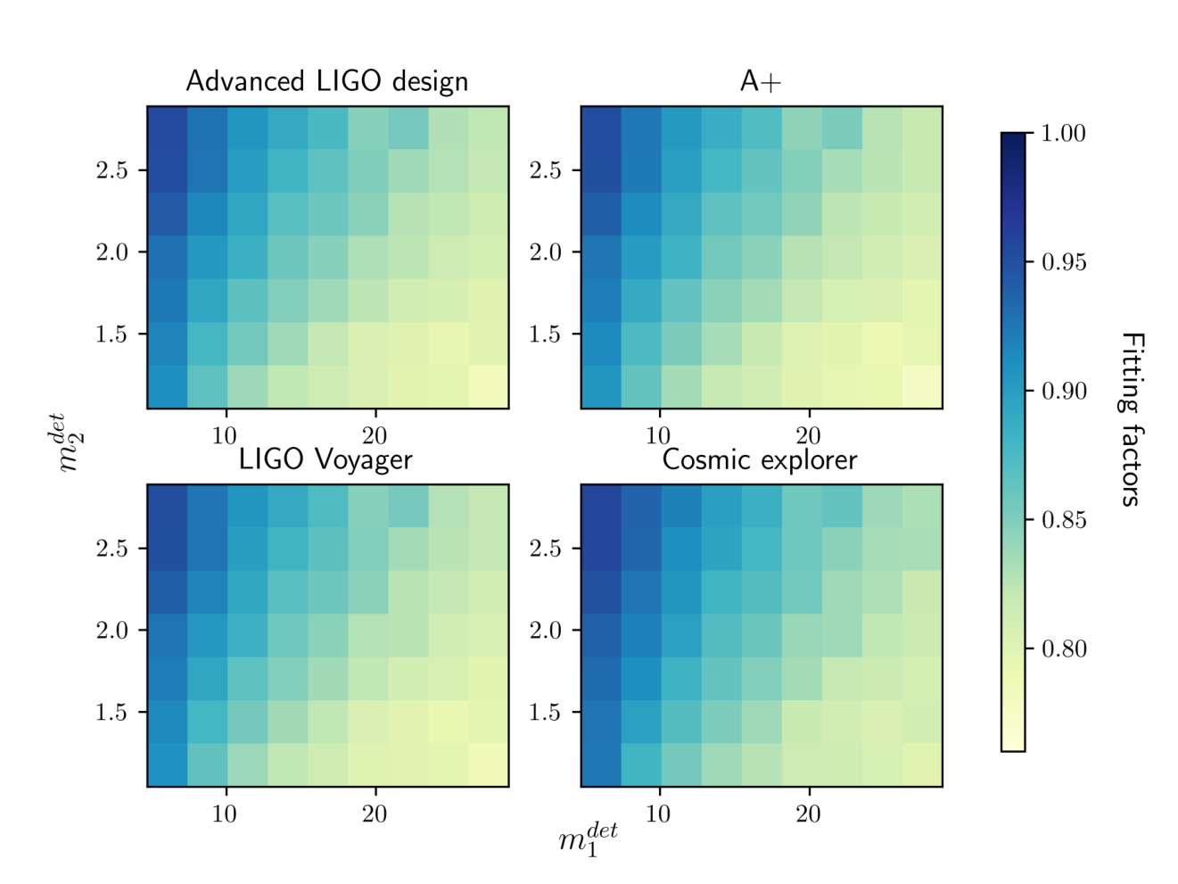
V.2 Number of Detectable Sources
In the previous section, we have studied the distribution of SNR fraction recovered by an aligned-spin search with respect to an idealized search that could recover all of a signal’s SNR. A real search will have an observational bias towards signals which are louder in comparison to others, which is not taken into account in the FF distribution. We can estimate the fraction of signals (SRF) that would instead be detected by an aligned-spin search w.r.t. an idealized search assuming a fixed SNR detection threshold. In Fig. 8 we show the distribution of the SRF for precessing signals with HMs as a function of for all four detector configurations. We notice a similar trend as the FF distribution; decreasing SRF with increasing mass-ratio of the binary. We find dominant mode aligned-spin template banks will miss up to of nonprecessing signals with HMs (not shown in the figure) and up to of the precessing systems assuming our fiducial population. These results hold for each detector configuration.

In practice, a real search that could incorporate the effects of precession and higher-order modes would incur a trials factor relative to the aligned-spin search; this has subdominant impact on the achievable sensitivity. To give an idea of the magnitude of this effect, we can approximate the relative sensitivity at a fixed false alarm rate, rather than at a fixed SNR threshold (see Eq. (13)). As a rough estimate, we take the appropriate , chosen to correspond to a given false alarm rate, from previous works which study developing HM Harry et al. 2018 and precessing searches Harry et al. 2016 as shown in the Table 3. Typically less than 1 in every 100 or 1000 years are used to claim a significant event Usman et al. 2016; Messick et al. 2017. We evaluate the relative sensitivity at these FARs of an aligned-spin search w.r.t. three different idealized searches: a HM search, a precessing, dominant-mode search, and a precessing higher-mode search. Since, precession effects dominate, we use the same effect threshold for the precessing cases.
In Fig. 9, we show the sensitivity relative to all three types of searches using the Advanced LIGO design noise curve as a function of (). Parameter regions where the relative sensitivity is depicts regions where aligned-spin search is less sensitive than the more advanced, ideal search. When searching for nonprecessing binaries, the aligned-spin bank is more sensitive than a naive search including HMs on average. But, an aligned-spin search loses up to of highly precessing () and highly asymmetric () NSBH binaries averaged over our fiducial population. We further classify sources based on separate mass-ratio regions, with [2, 5], [5, 10], [10, 15] or [15, 20], and plot the relative sensitivity for all the sub-populations as a function of () (left) and () (right) in Fig. 10. For low mass-ratio () binaries we find of highly precessing systems () will be missed by the aligned-spin search. On the other hand, in the high mass-ratio regions there is loss of () highly (moderately) precessing systems. Aligned-spin searches will also lose low mass-ratio binaries which are nearly edge-on. For high mass-ratios, we find a loss of () highly (moderately) precessing binaries. These results demonstrate a significant bias against highly precessing, or inclined systems; the development of a practical precessing search would increase the sensitivity to these sources.
| Bank | FAR | ||
|---|---|---|---|
| HMs | 9.37 | 9.7 | |
| Precession | 9.92 | 10.44 | |
| HMs with precession | 9.92 | 10.44 |


VI Developing a Fully Precessing Search
Our results indicate a necessity to implement a precessing search for the identified regions of poor sensitivity. One way of implementing a precessing search could be to use the same statistic as Eq. (9) and employ precessing templates. This approximation may not be valid while searching for signals with HMs or precession due to several reasons. For precessing signals, the two polarizations are not related by an overall phase shift , which is what enables the analytic maximization over extrinsic parameters. This is also true in the case of searching using HMs – as each mode has a unique phase dependence . In the case of a precessing, higher-mode search, both the orbital phase and the inclination of binary, which are typically considered extrinsic parameters, would now behave as intrinsic parameters. The ideal search would marginalize over all extrinsic and intrinsic parameters coherently for all observing detectors. However, a naive implementation would be significantly more expensive than the aligned-spin search due to the increase in the number of intrinsic parameters (spin vectors, orbital phase, inclination), and the need to numerically marginalize over the extrinsic parameters.
We can demonstrate the issue by comparing the match between the two polarizations for every source in our population using precessing signals with HMs. The value (1 - ) corresponds to the fraction of observed signal SNR lost as a result of approximation in Eq. (9); a value of corresponds to a loss of . In Fig. 11, we show the binned averaged value of the match as a function of () at Hz. From the plot, we observe the standard analytical maximization of extrinsic parameters is valid for searching non-precessing systems except when they are nearly edge-on. However, when searching for precessing systems the match decreases with increasing or . We measure a loss in SNR up to for nearly edge-on and up to for face-on/off precessing binaries. These results clearly invalidate the approximation in Eq. (9) and motivate the development of methods to efficiently marginalize over the extrinsic parameters of precessing sources.
Works have proposed new ways of approximating the optimal search statistic Harry et al. 2016; Harry et al. 2018. These search methods maximise the SNR over fewer extrinsic parameters than in Eq. (9) and across the remaining ones using a template bank with additional parameters; they also typically do this maximization incoherently between detectors. A generic approach to search for signals with HMs was introduced in Harry et al. 2018; the search maximised the SNR over () and uses two additional parameters () in the template bank. The same approach is employed in the first search for intermediate-mass BHs including HMs Chandra et al. 2022. Similarly, Harry et al. 2016 developed an approach to search for precessing signals; their statistic maximises the SNR over sky-parameters and imparts only one additional parameter to the template bank.

VII Conclusions and discussions
In this work we have studied the sensitivity of dominant mode, aligned-spin searches, as have been employed in past gravitational-wave surveys Abbott et al. 2021a; Olsen et al. 2022; Nitz et al. 2021, to a population of NSBH sources. We compare the number of sources an aligned spin search would detect at a fixed false alarm rate relative to idealized searches that incorporate either higher modes, precession, or both. In this study, we’ve used an estimate of the relative background of each search to account for the change in SNR threshold at a fixed false alarm rate; this could be further improved by a detailed study of precessing template bank generation, which we leave for future work.
We have modelled gravitational-wave signals using a recent waveform model which includes both the effects of precession and higher-order modes Pratten et al. 2021. The model has the largest potential systematics for highly precessing and asymmetrical-mass sources. While we do not expect qualitative changes to our results, improved models would help minimize potential systematic biases in precessing searches.
We find that the aligned spin searches are least effective in detecting sources with asymmetrical masses, large in-plane spins, or binaries with orientation close to edge-on. Dominant mode, aligned-spin searches lose up to of sources with mass-ratios and up to of highly precessing systems . We compare four different noise curves – Advanced LIGO design, A+, LIGO Voyager and Cosmic explorer and find that these results apply for each detector configuration we considered.
Real detector data contains non-Gaussian transient noise Abbott et al. 2016b; Davis et al. 2021; the impact of these artefacts is mitigated using a variety of vetoing methods Abbott et al. 2018b, including signal consistency tests Allen 2005; Abbott et al. 2018b. In this work we have not considered the impact of these vetoing methods. Since signal-consistency tests compare the expected signal to the data, it is possible that aligned-spin searches could misclassify signals with strong precession or HMs as noise. Therefore, we expect that in practice aligned-spin searches will have even stronger observational biases than presented here.
The detection of precessing systems or signals with higher-order modes provides better constraints of the component spins that carries signatures of the formation of compact-binary sources Gompertz et al. 2022; Stevenson et al. 2017; Talbot and Thrane 2017; Rodriguez et al. 2016; Johnson-McDaniel et al. 2022. We have identified regions of parameter space with significant bias against highly precessing systems. The poor sensitivity in these regions motivates the need to develop a search that can fully account for the gravitational-wave signal produced by precessing binaries. Precessing searches can pose computational challenges Harry et al. 2016 which might be overcome by implementing hierarchical strategies Dhurkunde et al. 2022; Soni et al. 2022. We expect that if we can solve these challenges, our results show that the solution will likely still apply for future detector configurations. Therefore, we strongly recommend a targeted precessing search in the identified regions with poor sensitivity.
Acknowledgements.
We would like to acknowledge Marlin Schäfer for reading the manuscript and for providing useful comments. We acknowledge the Max Planck Gesellschaft and the Atlas cluster computing team at Albert-Einstein Institute (AEI) Hannover for support.References
- Abbott et al. (2021a) R. Abbott et al. (LIGO Scientific, VIRGO, KAGRA), “GWTC-3: Compact Binary Coalescences Observed by LIGO and Virgo During the Second Part of the Third Observing Run,” (2021a), arXiv:2111.03606 [gr-qc] .
- Nitz et al. (2021) Alexander H. Nitz, Collin D. Capano, Sumit Kumar, Yi-Fan Wang, Shilpa Kastha, Marlin Schäfer, Rahul Dhurkunde, and Miriam Cabero, “3-OGC: Catalog of Gravitational Waves from Compact-binary Mergers,” Astrophys. J. 922, 76 (2021), arXiv:2105.09151 [astro-ph.HE] .
- Olsen et al. (2022) Seth Olsen, Tejaswi Venumadhav, Jonathan Mushkin, Javier Roulet, Barak Zackay, and Matias Zaldarriaga, “New binary black hole mergers in the LIGO–Virgo O3a data,” (2022), arXiv:2201.02252 [astro-ph.HE] .
- Aasi et al. (2015) J. Aasi et al. (LIGO Scientific), “Advanced LIGO,” Class. Quant. Grav. 32, 074001 (2015), arXiv:1411.4547 [gr-qc] .
- Acernese (2015) F. Acernese (Virgo), “The Advanced Virgo detector,” J. Phys. Conf. Ser. 610, 012014 (2015).
- Abbott et al. (2020a) B. P. Abbott et al. (LIGO Scientific, Virgo), “GW190425: Observation of a Compact Binary Coalescence with Total Mass ,” Astrophys. J. Lett. 892, L3 (2020a), arXiv:2001.01761 [astro-ph.HE] .
- Abbott et al. (2021b) R. Abbott et al. (LIGO Scientific, KAGRA, VIRGO), “Observation of Gravitational Waves from Two Neutron Star–Black Hole Coalescences,” Astrophys. J. Lett. 915, L5 (2021b), arXiv:2106.15163 [astro-ph.HE] .
- Margalit and Metzger (2017) Ben Margalit and Brian D. Metzger, “Constraining the Maximum Mass of Neutron Stars From Multi-Messenger Observations of GW170817,” Astrophys. J. Lett. 850, L19 (2017), arXiv:1710.05938 [astro-ph.HE] .
- Abbott et al. (2019a) B. P. Abbott et al. (LIGO Scientific, Virgo), “Binary Black Hole Population Properties Inferred from the First and Second Observing Runs of Advanced LIGO and Advanced Virgo,” Astrophys. J. Lett. 882, L24 (2019a), arXiv:1811.12940 [astro-ph.HE] .
- Gompertz et al. (2022) B. P. Gompertz, M. Nicholl, P. Schmidt, G. Pratten, and A. Vecchio, “Constraints on compact binary merger evolution from spin-orbit misalignment in gravitational-wave observations,” Mon. Not. Roy. Astron. Soc. 511, 1454–1461 (2022), arXiv:2108.10184 [astro-ph.HE] .
- Abbott et al. (2018a) B. P. Abbott et al. (KAGRA, LIGO Scientific, Virgo, VIRGO), “Prospects for observing and localizing gravitational-wave transients with Advanced LIGO, Advanced Virgo and KAGRA,” Living Rev. Rel. 21, 3 (2018a), arXiv:1304.0670 [gr-qc] .
- Cahillane and Mansell (2022) Craig Cahillane and Georgia Mansell, “Review of the Advanced LIGO Gravitational Wave Observatories Leading to Observing Run Four,” Galaxies 10, 36 (2022), arXiv:2202.00847 [gr-qc] .
- Adhikari et al. (2020) R. X. Adhikari et al. (LIGO), “A cryogenic silicon interferometer for gravitational-wave detection,” Class. Quant. Grav. 37, 165003 (2020), arXiv:2001.11173 [astro-ph.IM] .
- Reitze et al. (2019) David Reitze et al., “Cosmic Explorer: The U.S. Contribution to Gravitational-Wave Astronomy beyond LIGO,” Bull. Am. Astron. Soc. 51, 035 (2019), arXiv:1907.04833 [astro-ph.IM] .
- Belczynski et al. (2016) Krzysztof Belczynski, Serena Repetto, Daniel E. Holz, Richard O’Shaughnessy, Tomasz Bulik, Emanuele Berti, Christopher Fryer, and Michal Dominik, “Compact Binary Merger Rates: Comparison with LIGO/Virgo Upper Limits,” Astrophys. J. 819, 108 (2016), arXiv:1510.04615 [astro-ph.HE] .
- Abbott et al. (2016a) B. P. Abbott et al. (LIGO Scientific, Virgo), “Astrophysical Implications of the Binary Black-Hole Merger GW150914,” Astrophys. J. Lett. 818, L22 (2016a), arXiv:1602.03846 [astro-ph.HE] .
- Broekgaarden and Berger (2021) Floor S. Broekgaarden and Edo Berger, “Formation of the First Two Black Hole–Neutron Star Mergers (GW200115 and GW200105) from Isolated Binary Evolution,” Astrophys. J. Lett. 920, L13 (2021), arXiv:2108.05763 [astro-ph.HE] .
- Belczynski et al. (2010a) Krzysztof Belczynski, Michal Dominik, Tomasz Bulik, Richard O’Shaughnessy, Chris Fryer, and Daniel E. Holz, “The effect of metallicity on the detection prospects for gravitational waves,” Astrophys. J. Lett. 715, L138 (2010a), arXiv:1004.0386 [astro-ph.HE] .
- Dominik et al. (2012) Michal Dominik, Krzysztof Belczynski, Christopher Fryer, Daniel Holz, Emanuele Berti, Tomasz Bulik, Ilya Mandel, and Richard O’Shaughnessy, “Double Compact Objects I: The Significance of the Common Envelope on Merger Rates,” Astrophys. J. 759, 52 (2012), arXiv:1202.4901 [astro-ph.HE] .
- Pooley et al. (2003) D. Pooley et al., “Dynamical formation of close binary systems in globular clusters,” Astrophys. J. Lett. 591, L131–L134 (2003), arXiv:astro-ph/0305003 .
- Rodriguez et al. (2015) Carl L. Rodriguez, Meagan Morscher, Bharath Pattabiraman, Sourav Chatterjee, Carl-Johan Haster, and Frederic A. Rasio, “Binary Black Hole Mergers from Globular Clusters: Implications for Advanced LIGO,” Phys. Rev. Lett. 115, 051101 (2015), [Erratum: Phys.Rev.Lett. 116, 029901 (2016)], arXiv:1505.00792 [astro-ph.HE] .
- Stevenson et al. (2017) Simon Stevenson, Christopher P. L. Berry, and Ilya Mandel, “Hierarchical analysis of gravitational-wave measurements of binary black hole spin–orbit misalignments,” Mon. Not. Roy. Astron. Soc. 471, 2801–2811 (2017), arXiv:1703.06873 [astro-ph.HE] .
- Talbot and Thrane (2017) Colm Talbot and Eric Thrane, “Determining the population properties of spinning black holes,” Phys. Rev. D 96, 023012 (2017), arXiv:1704.08370 [astro-ph.HE] .
- Rodriguez et al. (2016) Carl L. Rodriguez, Michael Zevin, Chris Pankow, Vasilliki Kalogera, and Frederic A. Rasio, “Illuminating Black Hole Binary Formation Channels with Spins in Advanced LIGO,” Astrophys. J. Lett. 832, L2 (2016), arXiv:1609.05916 [astro-ph.HE] .
- Johnson-McDaniel et al. (2022) Nathan K. Johnson-McDaniel, Sumeet Kulkarni, and Anuradha Gupta, “Inferring spin tilts at formation from gravitational wave observations of binary black holes: Interfacing precession-averaged and orbit-averaged spin evolution,” Phys. Rev. D 106, 023001 (2022), arXiv:2107.11902 [astro-ph.HE] .
- Krishnendu and Ohme (2022) N. V. Krishnendu and Frank Ohme, “Interplay of spin-precession and higher harmonics in the parameter estimation of binary black holes,” Phys. Rev. D 105, 064012 (2022), arXiv:2110.00766 [gr-qc] .
- Hannam et al. (2021) Mark Hannam, Charlie Hoy, Jonathan E. Thompson, Stephen Fairhurst, and Vivien Raymond (VIRGO), “Measurement of general-relativistic precession in a black-hole binary,” (2021), arXiv:2112.11300 [gr-qc] .
- Abbott et al. (2020b) R. Abbott et al. (LIGO Scientific, Virgo), “GW190412: Observation of a Binary-Black-Hole Coalescence with Asymmetric Masses,” Phys. Rev. D 102, 043015 (2020b), arXiv:2004.08342 [astro-ph.HE] .
- Abbott et al. (2020c) R. Abbott et al. (LIGO Scientific, Virgo), “GW190814: Gravitational Waves from the Coalescence of a 23 Solar Mass Black Hole with a 2.6 Solar Mass Compact Object,” Astrophys. J. Lett. 896, L44 (2020c), arXiv:2006.12611 [astro-ph.HE] .
- Capano et al. (2021) Collin D. Capano, Miriam Cabero, Julian Westerweck, Jahed Abedi, Shilpa Kastha, Alexander H. Nitz, Alex B. Nielsen, and Badri Krishnan, “Observation of a multimode quasi-normal spectrum from a perturbed black hole,” (2021), arXiv:2105.05238 [gr-qc] .
- Broekgaarden et al. (2021a) Floor S. Broekgaarden et al., “Impact of Massive Binary Star and Cosmic Evolution on Gravitational Wave Observations II: Double Compact Object Rates and Properties,” (2021a), arXiv:2112.05763 [astro-ph.HE] .
- Fryer and Kalogera (2001) Chris L. Fryer and Vassiliki Kalogera, “Theoretical black hole mass distributions,” Astrophys. J. 554, 548–560 (2001), arXiv:astro-ph/9911312 .
- Belczynski et al. (2010b) Krzysztof Belczynski, Tomasz Bulik, Chris L. Fryer, Ashley Ruiter, Jorick S. Vink, and Jarrod R. Hurley, “On The Maximum Mass of Stellar Black Holes,” Astrophys. J. 714, 1217–1226 (2010b), arXiv:0904.2784 [astro-ph.SR] .
- Lyne and Lorimer (1994) A. G. Lyne and D. R. Lorimer, “High birth velocities of radio pulsars,” Nature 369, 127 (1994).
- Janka (2013) H. Thomas Janka, “Natal Kicks of Stellar-Mass Black Holes by Asymmetric Mass Ejection in Fallback Supernovae,” Mon. Not. Roy. Astron. Soc. 434, 1355 (2013), arXiv:1306.0007 [astro-ph.SR] .
- Broekgaarden et al. (2021b) Floor S. Broekgaarden, Edo Berger, Coenraad J. Neijssel, Alejandro Vigna-Gómez, Debatri Chattopadhyay, Simon Stevenson, Martyna Chruslinska, Stephen Justham, Selma E. de Mink, and Ilya Mandel, “Impact of massive binary star and cosmic evolution on gravitational wave observations I: black hole–neutron star mergers,” Mon. Not. Roy. Astron. Soc. 508, 5028–5063 (2021b), arXiv:2103.02608 [astro-ph.HE] .
- Gupta et al. (2017) Anuradha Gupta, K. G. Arun, and B. S. Sathyaprakash, “Implications of Binary Black Hole Detections on the Merger Rates of Double Neutron Stars and Neutron Star–Black Holes,” Astrophys. J. Lett. 849, L14 (2017), arXiv:1708.03939 [astro-ph.IM] .
- Harry et al. (2014) Ian W. Harry, Alexander H. Nitz, Duncan A. Brown, Andrew P. Lundgren, Evan Ochsner, and Drew Keppel, “Investigating the effect of precession on searches for neutron-star-black-hole binaries with Advanced LIGO,” Phys. Rev. D 89, 024010 (2014), arXiv:1307.3562 [gr-qc] .
- Usman et al. (2016) Samantha A. Usman et al., “The PyCBC search for gravitational waves from compact binary coalescence,” Class. Quant. Grav. 33, 215004 (2016), arXiv:1508.02357 [gr-qc] .
- Messick et al. (2017) Cody Messick et al., “Analysis Framework for the Prompt Discovery of Compact Binary Mergers in Gravitational-wave Data,” Phys. Rev. D 95, 042001 (2017), arXiv:1604.04324 [astro-ph.IM] .
- Aubin et al. (2021) F. Aubin et al., “The MBTA pipeline for detecting compact binary coalescences in the third LIGO–Virgo observing run,” Class. Quant. Grav. 38, 095004 (2021), arXiv:2012.11512 [gr-qc] .
- Hooper et al. (2012) Shaun Hooper, Shin Kee Chung, Jing Luan, David Blair, Yanbei Chen, and Linqing Wen, “Summed Parallel Infinite Impulse Response (SPIIR) Filters For Low-Latency Gravitational Wave Detection,” Phys. Rev. D 86, 024012 (2012), arXiv:1108.3186 [gr-qc] .
- Pratten et al. (2021) Geraint Pratten et al., “Computationally efficient models for the dominant and subdominant harmonic modes of precessing binary black holes,” Phys. Rev. D 103, 104056 (2021), arXiv:2004.06503 [gr-qc] .
- Ossokine et al. (2020) Serguei Ossokine et al., “Multipolar Effective-One-Body Waveforms for Precessing Binary Black Holes: Construction and Validation,” Phys. Rev. D 102, 044055 (2020), arXiv:2004.09442 [gr-qc] .
- Harry et al. (2016) Ian Harry, Stephen Privitera, Alejandro Bohé, and Alessandra Buonanno, “Searching for Gravitational Waves from Compact Binaries with Precessing Spins,” Phys. Rev. D 94, 024012 (2016), arXiv:1603.02444 [gr-qc] .
- Harry et al. (2018) Ian Harry, Juan Calderón Bustillo, and Alex Nitz, “Searching for the full symphony of black hole binary mergers,” Phys. Rev. D 97, 023004 (2018), arXiv:1709.09181 [gr-qc] .
- Chandra et al. (2022) Koustav Chandra, Juan Calderón Bustillo, Archana Pai, and Ian Harry, “First gravitational-wave search for intermediate-mass black hole mergers with higher order harmonics,” (2022), arXiv:2207.01654 [gr-qc] .
- Calderón Bustillo et al. (2017) Juan Calderón Bustillo, Pablo Laguna, and Deirdre Shoemaker, “Detectability of gravitational waves from binary black holes: Impact of precession and higher modes,” Phys. Rev. D 95, 104038 (2017), arXiv:1612.02340 [gr-qc] .
- Blackman et al. (2017) Jonathan Blackman, Scott E. Field, Mark A. Scheel, Chad R. Galley, Christian D. Ott, Michael Boyle, Lawrence E. Kidder, Harald P. Pfeiffer, and Béla Szilágyi, “Numerical relativity waveform surrogate model for generically precessing binary black hole mergers,” Phys. Rev. D 96, 024058 (2017), arXiv:1705.07089 [gr-qc] .
- Mills and Fairhurst (2021) Cameron Mills and Stephen Fairhurst, “Measuring gravitational-wave higher-order multipoles,” Phys. Rev. D 103, 024042 (2021), arXiv:2007.04313 [gr-qc] .
- Apostolatos et al. (1994) Theocharis A. Apostolatos, Curt Cutler, Gerald J. Sussman, and Kip S. Thorne, “Spin induced orbital precession and its modulation of the gravitational wave forms from merging binaries,” Phys. Rev. D 49, 6274–6297 (1994).
- Ajith et al. (2011) P. Ajith et al., “Inspiral-merger-ringdown waveforms for black-hole binaries with non-precessing spins,” Phys. Rev. Lett. 106, 241101 (2011), arXiv:0909.2867 [gr-qc] .
- Schmidt et al. (2015) Patricia Schmidt, Frank Ohme, and Mark Hannam, “Towards models of gravitational waveforms from generic binaries II: Modelling precession effects with a single effective precession parameter,” Phys. Rev. D 91, 024043 (2015), arXiv:1408.1810 [gr-qc] .
- Estellés et al. (2022) Héctor Estellés et al., “A Detailed Analysis of GW190521 with Phenomenological Waveform Models,” Astrophys. J. 924, 79 (2022), arXiv:2105.06360 [gr-qc] .
- Tiwari (2022) Vaibhav Tiwari, “Exploring Features in the Binary Black Hole Population,” Astrophys. J. 928, 155 (2022), arXiv:2111.13991 [astro-ph.HE] .
- Zhu et al. (2022) Jin-Ping Zhu, Shichao Wu, Ying Qin, Bing Zhang, He Gao, and Zhoujian Cao, “Population Properties of Gravitational-wave Neutron Star–Black Hole Mergers,” Astrophys. J. 928, 167 (2022), arXiv:2112.02605 [astro-ph.HE] .
- Nitz et al. (2019) Alexander H. Nitz, Collin Capano, Alex B. Nielsen, Steven Reyes, Rebecca White, Duncan A. Brown, and Badri Krishnan, “1-OGC: The first open gravitational-wave catalog of binary mergers from analysis of public Advanced LIGO data,” Astrophys. J. 872, 195 (2019), arXiv:1811.01921 [gr-qc] .
- Abbott et al. (2018b) B P Abbott et al. (LIGO Scientific, Virgo), “Effects of data quality vetoes on a search for compact binary coalescences in Advanced LIGO’s first observing run,” Class. Quant. Grav. 35, 065010 (2018b), arXiv:1710.02185 [gr-qc] .
- Allen (2005) Bruce Allen, “ time-frequency discriminator for gravitational wave detection,” Phys. Rev. D 71, 062001 (2005), arXiv:gr-qc/0405045 .
- Abbott et al. (2016b) B. P. Abbott et al. (LIGO Scientific, Virgo), “Characterization of transient noise in Advanced LIGO relevant to gravitational wave signal GW150914,” Class. Quant. Grav. 33, 134001 (2016b), arXiv:1602.03844 [gr-qc] .
- Davis et al. (2021) Derek Davis et al. (LIGO), “LIGO detector characterization in the second and third observing runs,” Class. Quant. Grav. 38, 135014 (2021), arXiv:2101.11673 [astro-ph.IM] .
- Abbott et al. (2019b) B. P. Abbott et al. (LIGO Scientific, Virgo), “GWTC-1: A Gravitational-Wave Transient Catalog of Compact Binary Mergers Observed by LIGO and Virgo during the First and Second Observing Runs,” Phys. Rev. X 9, 031040 (2019b), arXiv:1811.12907 [astro-ph.HE] .
- Allen et al. (2012) Bruce Allen, Warren G. Anderson, Patrick R. Brady, Duncan A. Brown, and Jolien D. E. Creighton, “FINDCHIRP: An Algorithm for detection of gravitational waves from inspiraling compact binaries,” Phys. Rev. D 85, 122006 (2012), arXiv:gr-qc/0509116 .
- Owen and Sathyaprakash (1999) Benjamin J. Owen and B. S. Sathyaprakash, “Matched filtering of gravitational waves from inspiraling compact binaries: Computational cost and template placement,” Phys. Rev. D 60, 022002 (1999), arXiv:gr-qc/9808076 .
- Babak et al. (2006) S. Babak, R. Balasubramanian, D. Churches, T. Cokelaer, and B. S. Sathyaprakash, “A Template bank to search for gravitational waves from inspiralling compact binaries. I. Physical models,” Class. Quant. Grav. 23, 5477–5504 (2006), arXiv:gr-qc/0604037 .
- Harry et al. (2009) Ian W. Harry, Bruce Allen, and B. S. Sathyaprakash, “A Stochastic template placement algorithm for gravitational wave data analysis,” Phys. Rev. D 80, 104014 (2009), arXiv:0908.2090 [gr-qc] .
- Babak (2008) Stanislav Babak, “Building a stochastic template bank for detecting massive black hole binaries,” Class. Quant. Grav. 25, 195011 (2008), arXiv:0801.4070 [gr-qc] .
- Roy et al. (2019) Soumen Roy, Anand S. Sengupta, and Parameswaran Ajith, “Effectual template banks for upcoming compact binary searches in Advanced-LIGO and Virgo data,” Phys. Rev. D 99, 024048 (2019), arXiv:1711.08743 [gr-qc] .
- Capano et al. (2016) Collin Capano, Ian Harry, Stephen Privitera, and Alessandra Buonanno, “Implementing a search for gravitational waves from binary black holes with nonprecessing spin,” Phys. Rev. D 93, 124007 (2016), arXiv:1602.03509 [gr-qc] .
- Lenon et al. (2021) Amber K. Lenon, Duncan A. Brown, and Alexander H. Nitz, “Eccentric binary neutron star search prospects for Cosmic Explorer,” Phys. Rev. D 104, 063011 (2021), arXiv:2103.14088 [astro-ph.HE] .
- Buonanno et al. (2003) Alessandra Buonanno, Yan-bei Chen, and Michele Vallisneri, “Detecting gravitational waves from precessing binaries of spinning compact objects: Adiabatic limit,” Phys. Rev. D 67, 104025 (2003), [Erratum: Phys.Rev.D 74, 029904 (2006)], arXiv:gr-qc/0211087 .
- Husa et al. (2016) Sascha Husa, Sebastian Khan, Mark Hannam, Michael Pürrer, Frank Ohme, Xisco Jiménez Forteza, and Alejandro Bohé, “Frequency-domain gravitational waves from nonprecessing black-hole binaries. I. New numerical waveforms and anatomy of the signal,” Phys. Rev. D 93, 044006 (2016), arXiv:1508.07250 [gr-qc] .
- Khan et al. (2016) Sebastian Khan, Sascha Husa, Mark Hannam, Frank Ohme, Michael Pürrer, Xisco Jiménez Forteza, and Alejandro Bohé, “Frequency-domain gravitational waves from nonprecessing black-hole binaries. II. A phenomenological model for the advanced detector era,” Phys. Rev. D 93, 044007 (2016), arXiv:1508.07253 [gr-qc] .
- Dhurkunde et al. (2022) Rahul Dhurkunde, Henning Fehrmann, and Alexander H. Nitz, “Hierarchical approach to matched filtering using a reduced basis,” Phys. Rev. D 105, 103001 (2022), arXiv:2110.13115 [astro-ph.IM] .
- Soni et al. (2022) Kanchan Soni, Bhooshan Uday Gadre, Sanjit Mitra, and Sanjeev Dhurandhar, “Hierarchical search for compact binary coalescences in the Advanced LIGO’s first two observing runs,” Phys. Rev. D 105, 064005 (2022), arXiv:2106.08925 [gr-qc] .