Post-processing of coronary and myocardial spatial data

The collection of segments can be hierarchically ordered according to the generation to which they belong. In addition to being helpful when removing spuriously short segments, generation affiliation can be used as a filter for segments. In either case, it is necessary to sort the nodes into generations. The $0^{\rm th}$ generation contains the segment with the inlet node. Given the $i$ sorted generations, the $(i+1)^{\rm st}$ generation contains segments that begin with the final nodes of the $i^{\rm th}$ generation. It is possible to sort any subset of the segments into generations. The 3910 segments in this data set can be sorted into 42 generations.

A coronal projection (onto the $(x,y)$-plane) of the first four generations is shown in Fig. 2a. From the figure, it appears as if the vessels of generations 1 and 2 arise directly from the $0^{\rm th}$ generation. This occurs due to the presence of a spuriously short segment in $1^{\rm st}$ generation that is too short to be seen on such a scale. This short segment can be clearly seen in Fig. 2b which is a 30 times magnification of Fig. 2a centred at the first junction. The spuriously short segment contains only 2 nodes, while its sibling contains 51 nodes, and its daughters contain 9 and 39 nodes. In addition, the radii at both nodes of the segment are greater than its length. Given this, it is reasonable to presume that the short segment is an artifact of the initial skeletonisation. As discussed above, the initial node of spuriously short segments is appended to its daughter segments, so that the daughter segments are effectively moved up one generation, and the spuriously short segment can be removed without loss of information. The impact of this can be seen by comparing Fig. 2b and Fig. 2d. It is by this procedure that we transform a pseudotrifurcation into a trifurcation. This is easily generalisable to higher junction orders.

Upon removing the 761 short segments, there are 3149 segments in 32 generations.

It is not clear if segments containing 3 nodes should be considered as spuriously short as none of the 381 such segments has Euclidean arc-length less than its mean radius. As such, no segments of length 3 or longer are considered spuriously short.

One possible application of the trees generated using the current analysis is in haemodynamic flow models. In these, there is a trade off between model fidelity and computational cost. Flow simulations in trees with more branches are more computationally costly than those with fewer branches, not just because of the branch count itself, but because the junctions between vessels can be expensive to match [19]. In two-sided models, coupling arterial to venous networks, such as those discussed by Mackenzie [19] and Qureshi et al. [11], a single additional generation of vessels can as much as quadruple computational costs. Further, as shown by Mackenzie [19], the flow in all vessels is correlated to the total volume of the network. In the tree, segment volume typically decreases as a function of of increasing distance from the root. In this tree, the number of vessels per generation is increasing until the 16^th generation and contains a total of 1927 segments. Given this, it is reasonable to ask what the maximum number of generations that ought be included in the tree is. One possible metric that can be used to help answer this question is the information density, $I$. Let $n$ be the number of segments per generation and $v$ be the total volume of the segments in a generation. Generations are indexed by a non-negative integer $i$. Information density is defined to be $I(i)\coloneqq v(i)/n(i)$ in the $i^{\rm th}$ generation. Figure 3 shows graphs of $n(i)$, $v(i)$, and $I(i)$ as discrete functions of $i$. Information density has a peak when $i=2$ and decreasingly decreasing from then on. The additional information gained by adding another generation can be quantified by finding $\Delta I(i+1)=I(i+1)-I(i)$ for $i\geq 0$. This peaks at $i=0$, between the 0^th and 1^st generations. We choose the threshold on $\Delta I$ for excluding a generation be two orders of magnitude lower than its peak, i.e. all generations after the first for which

should not be included. This happens first when $i=5$. If one wishes to use a generation based filter to reduce the number of segments eligible for inclusion in a tree, a reasonable choice for an upper bound based on this metric is 5. The information density is used as a proxy for the balance between computational domain fidelity and computational time as a voluminous generation of few vessels should certainly be included in the computational domain, but a generation containing numerous small vessels will have a significant impact on computational time without a significant impact on simulation results. The first 8 generations of the tree make up 51% of the total volume of the tree. Hence, including more than 8 generations may increase the fidelity of a fluids simulation (subject to modelling assumptions), but beyond 8 generations computational costs will increase more quickly that computational domain fidelity increases.

Radius is another natural metric by which to exclude a segment from the principal pathway. Every segment contains at least two nodes, and all nodes have an associated radius value. In radius-based pruning, a radius threshold is given. The radii in this coronary tree are not monotonically deceasing with distance from the root node, so applying a radius-based pruning condition is not as straightforward as finding the segments that contain a node that exceeds a threshold. There are several possible ways to apply a radius-based pruning condition. Here, we discuss a mean radius condition, a proportional condition, and a single-node condition.

• Mean Radius: In a mean radius condition, each segment is considered individually, and if the mean radius of the nodes in that segment exceeds a given threshold, then the segment is eligible for inclusion in the final tree. This method may be sensitive to spurious radius values that skew the distribution of a vessel. Comparing, for example, the mean and median radius in each segment may highlight segments in which this is an issue. A tree filtered by mean radius can be seen in Fig. 5a.

• Proportional Threshold: If a certain proportion of nodes in a segment have a radius greater than the given threshold, then that segment is eligible for inclusion in the final tree. This condition may be ill suited to dealing with segments that contain few nodes.

• Single Node: If a single node in a segment has an associated radius that exceeds the threshold, then it is eligible for inclusion in the final tree. Including any segment with at least one node with a radius that exceeds the threshold will lead to the inclusion of more vessels than the above-described mean radius condition. However, it will be sensitive to the existence of spuriously small radii values. A single node-filtered tree can be seen in Fig. 5c.

Other radius-based conditions exist, and it is certainly possible to apply multiple conditions within a single tree based, for example, on segment length. A proportional-threshold filtered tree can be seen in Fig. 5b. In general, we use a proportional threshold and require that at least 75% of the nodes in a given segment exceed the lower radius bound to be eligible for inclusion. This proportion was chosen after some experimentation to avoid setting an overly strict or overly lenient inclusion criterion. An overly strict criterion may limit the variety of trees that could be produced and an overly lenient criterion would produce trees that do not necessarily conform to the desired constraints.

Figure 4 shows the Mercator projection of the first six generations of segments. In particular, Fig. 4b shows the connected tree of segments in the first six generations that have a mean radius greater than 0.6 mm. Generations 0 through 6 contain 162 segments, 28 of which meet the radius condition.

Rendering 3D spatial data in a 2D medium may lead to difficulty in the interpretation of the figures. To render the 3D trees here, we use a Mercator projection [29] that preserves the branching structure of the tree but not the length of the segments.

As radius is not monotonically decreasing with distance from the root node, some segments give rise to others in which the radius in the daughter segment exceeds that of the parent. As such, radius-based filtration methods give a set of segments that meet the given criterion for generation affiliation and radius but are not necessarily accessible from the inlet of the tree since intermediate segments have been filtered out. This results in a tree in which some segments are not connected to the component contained in the inlet node. A principal pathway must be a tree in which all segments are connected to the component containing the inlet node. Hence, if pruning results in segments becoming disconnected from the inlet, a principal pathway can be obtained in, at least, one of two ways: by removing the components that are disconnected from the component containing the inlet node; or by reconnecting the disconnected segments to the component containing the inlet node.

The former is straightforward if the generations of all segments have already been computed. Given a collection of segments, it is easy to construct sets that contain the initial $S_{i}$ and final $S_{f}$, nodes of all segments. In a connected tree, $S_{i}\setminus S_{f}$ should contain only the inlet node; any other node that is returned lies at the inlet of a disconnected segment that should be removed. Recompute $S_{i}$, $S_{f}$, and $S_{i}\setminus S_{f}$ while $|S_{i}\setminus S_{f}|>1$. This is the procedure used to remove the highlighted segments in cyan seen in Figs. 5.

As can be seen in Fig. 4b, there appear to be segments that give rise to exactly one other vessel. As mentioned, much of the computational time spent during flow simulations with these networks is spent on matching the boundaries between vessels, hence it is computationally advantageous to join a parent segment and its single child to form a one longer segment. Such a join is advantageous as it reduces the complexity of the tree structure without loss of information.

Figure 4c shows the tree from Fig. 4b in which series joins have been made. The resulting tree (Fig. 4c) contains 16 segments.

Earlier, we saw that all segments containing two nodes are considered to be spuriously short. This is not the only circumstance under which it might be useful to remove a short segment. In Fig. 4c there is an instance in which a long segment (in generation 3) appears to give rise to exactly one other vessel (in generation 4) – it can be seen in the lower right of the panel of Fig. 4c. However, this cannot be the case that such vessels have been concatenated to form a single longer vessel. It transpires that the vessel of generation 3 gives rise to two vessels containing 21 nodes (which is appreciated) and 3 nodes (which cannot be appreciated). The sibling containing 3 nodes is deemed to be short and is removed from the tree. Once segment concatenation has been performed again, we obtain the tree seen in Fig. 4d.

Currently, there is no clear optimal criterion for the additional removal of short segments from a tree. More work is needed to establish this condition. At present, a segment is removed if it contains fewer than 5 nodes and gives rise to no further segments that are eligible for inclusion.

The Strahler order of a tree is a metric of its branching complexity. The metric was first developed by Horton [30] and later by Strahler [31, 32] for applications in hydrology. Strahler ordering has been widely applied to vascular trees; see, for example, [33, 13, 34, 21]. Strahler numbers are assigned from the bottom up as follows:

1. 1.

   if a branch has no children, it is given order 1

2. 2.

   if a branch has a child of order $n$ and all other children have order less than $n$, then give the branch order $n$

3. 3.

   if the branch has two or more children of order $n$, and no children with greater order, the Strahler order is $n+1$.

Figure 6 shows the largest segments of the tree that belong to orders 3 through 7. Vessels of orders 1 and 2 are omitted from the figure as they are sufficiently numerous to occlude other vessels in the tree.

Briefly, we have taken a given graph comprised of nodes, edges, and a radius measurement at every node and constructed a simplified graph by creating segments that run between two junction nodes or a junction node and a terminal node. The segments are sorted into generations, after which spuriously short segments are removed. The resulting tree can be pruned to conform to given criteria on, for example, the generation, Strahler order, or radius of a given vessel. If such filtration results in a disconnected tree, then the disconnected segments are discarded. If a terminal segment is very short, it is discarded. If a branch gives rise to a single daughter segment, these are concatenated to form a single longer segment that contains all the nodes of the two segments that were concatenated.

By the definition of the septum here, there are nodes that belong to the septum and the ventricle, but the tree does not reach part of the ventricle. Mathematically this is $S\subset V$ and $\mathcal{S}\cap\mathcal{T}=\emptyset$, so $\mathcal{S}\subset\mathcal{V}\setminus\mathcal{T}$ where $S$ is the collection of septal nodes, and $\mathcal{S}$ is the septal region. Figure 7c shows the regions $\mathcal{T}$ (yellow) and $\mathcal{V}$ (cyan); the intersection $\mathcal{T}\cap\mathcal{V}$ can be seen in grey. There are disjoint subregions that comprise the unperfused region $\mathcal{T}\setminus\mathcal{V}$ seen in Fig. 7d. The largest of these $\mathcal{S}$, highlighted in green in Fig. 8, is isolated manually using a data brushing tool.

Although the depictions here have been in $\mathbb{R}^{2}$, as the regions all belong to $\mathbb{R}^{3}$ by finding $\mathcal{S}\in\mathbb{R}^{2}$, $\mathcal{S}\in\mathbb{R}^{3}$ is now also found.

Let the region of the left ventricle that is perfused from the left coronary tree be $\mathcal{L}=\mathcal{V}\setminus\mathcal{S}$. As can be seen in Fig. 8, there are unperfused regions that are not connected to the septum. These are assumed to be perfused and arise due to imaging constraints.

Principal pathways are generated from vascular data using the methods described in Subsections 2.1 and 2.2. Let the principal pathway with $n$ terminal branches be denoted by $B_{n}\subset T,n\in\mathbb{Z}_{\geq 2}$. The perfused ventricular region $\mathcal{L}$ should be divided into subdomains $n$. Here, this division is informed by the vasculature. The set of terminal nodes of $B_{n}$ is $\partial B_{n}$, and the principal pathway is the region $\mathcal{B}_{n}$.

Let the $n$ subregions of $\mathcal{L}$ be denoted $\mathcal{S}_{i}$, $i=1,\dots,n$. Here, the $i^{\rm th}$ subregion is perfused from the $i^{\rm th}$ terminal artery of $B_{n}$, which is the element $i^{\rm th}$ of $\partial B_{n}$ is ${\partial B_{n}}_{i}$. By construction, the ventricle $\mathcal{V}$ is the union of the subdomains

where the septum $S$ is the subdomain $0^{\rm th}$ $S_{0}$. The node ${\partial B_{n}}_{0}$ is the inlet node.

To generate the regions $\mathcal{S}_{i}$, $i=1,\dots n$ based on the vascular tree, the nodes in $T$ downstream of ${\partial B_{n}}_{i}$ must be found for each value of $i=1,\dots,n$. The set $U=T\setminus B_{n}$ contains all nodes not in the principal pathway and, therefore, contains all nodes downstream of the principal pathway. The set $U$ also contains nodes that cannot be reached from the terminii of the principal pathways.

It is straightforward to determine which nodes in $U$ lie downstream of the terminal nodes in a given principal pathway. We do this considering the path between the initial node and a given node in $U$. If the path contains the index of a terminal node of the principal pathway, the given node is downstream of that terminal node and hence is perfused from the terminal branch to which it belongs. If the given node lies downstream of the terminal node of the $i^{\rm th}$ terminal segment of the principal pathway, sort it into a set $M_{i}$ and remove it from $U$, otherwise it is left in $U$. Repeat this for all nodes in $U$ until they have all been considered. No node need be considered twice. This is called the terminal node search. The subsets $M_{i}\subset U$, $i=1,2,...,n$, $n=6$, contain discrete spatial nodes and are shown in Fig. 9a. After constructing the sets $M_{i}$, there may still be nodes in $U$, now considered to be the unreachable nodes; these are shown as cyan dots in Fig. 9a. The terminii of the principal pathway from which the sets $M_{i}$ are sought are shown as red triangles in Fig. 9a. The sets $M_{i}$, $i\in[1,n]$, $n=6$ are also shown in Fig. 9c together with the principal pathway.

In the illustrative case $B_{6}$, there are 4821 nodes remaining in $U$ of an original 17448 shown as cyan dots in Fig. 9a. It seems reasonable that a collection of nodes that branch directly from a terminal segment (but not the terminus) should be considered to be perfused by that segment. This is the rationale for moving the seed points from which $U$ and $M_{i}$ are generated to the initial nodes in each terminal branch. Denote the resulting vascular compartments as $M_{i}^{\prime}$ and note that in the case of $B_{6}$, there are no unassigned nodes in $U^{\prime}$ when looking for downstream nodes from the terminal branches. It is not always true that $|U^{\prime}|=0$ (as in the case of $B_{8}$), but it is guaranteed that $|U^{\prime}|\leq|U|$. This is called the initial node search.

The discrete nodes of the sets $M_{i}^{\prime}$ can be used to define the regions that these nodes occupy called $\mathcal{M}_{i}^{\prime}$. These are the regions of the vasculature that are perfused from a given artery of the principal pathway. These regions and the principal pathway are shown in Fig. 10a. Each of the regions $\mathcal{M}_{i}$ intersects with the ventricular region $\mathcal{V}$. We call this intersection $\mathcal{S}_{i}=\mathcal{V}\cap\mathcal{M}_{i}$. This is the region within the ventricle that is perfused from the $i^{\rm th}$ terminal segment of the principal pathway. In practice, this is done by constructing $\partial M_{i}$ and finding the nodes $S$ that lie within $\partial M_{i}$[35] and assigning these to $\mathcal{S}_{i}$. The elements of $S_{i}=V\cap\mathcal{M}_{i}$ within each region $\mathcal{M}_{i}$ can be seen in Fig. 10b. The boundaries $\partial S_{i}$ are shown in Fig. 10c.

With the modelling assumption that no point in the ventricle can be perfused from two different terminal arteries, then the restriction that the regions $\mathcal{S}_{i}$ are disjoint must be imposed. Hence, for each $i\in[1,n]$, redefine

Now, by construction the ventricle has been divided into $n+2$ subregions, so

where $\mathcal{S}_{*}$ is a disjoint region comprised of nodes that have yet to be assigned to their final subdomain in order that the whole ventricle may be perfused. In the case of $n=6$, there are 665 of the 17,440 nodes in the volume filling point cloud that have been double assigned and 3134 that have not been assigned in this initial stage. Hence, $|S_{*}|=3799$ which must be assigned to one of $S_{i}$, $i\in[0,6]$.

The set $S_{*}$ contains nodes that belong to a volume filling point cloud that describes the ventricle but have not been assigned to a subdomain $S_{i}$, $i\in[0,n]$. All nodes of the volume-filling cloud must be assigned to one of $S_{i}$, $i\in[0,n]$. In order to assign the nodes of $S_{*}$ to a subdomain, we consider the neighbouring nodes according to the volume-filling tetrahedral mesh.

The region $\mathcal{V}$ is represented by a cloud of volume-filling points and associated tetrahedral. Let $E=\{a,b,c,d\}$ be a mesh element that joins nodes with indices $a$, $b$, $c$ and $d$ in a tetrahedron. Suppose that element $E$ is associated with the subdomains by $N=\{F,-1,F,F\}$, then we say that $a,~c,~d$ lies in the subdomain $F$ and the node $b$ has not yet been assigned. As three neighbours of $b$ belong to $F$, assign $b$ to $F$. There is a subdomain list $N$ for each element $N$, so when $b$ is assigned to $F$ all lists $N$ must be updated to reflect that $b$ now lies in $F$. After repeating reassignment for each element, the subdomains have collectively gained nodes, so there are more elements $E$ with lists $N$ that meet the criterion for reassignment. Repeat this process for the list of elements that contain unassigned nodes until no elements that meet the assignment criteria remain.

In the case of $6+1$ subdomains, the first run of the algorithm described above leads to the assignment of 2,099 nodes. The second run assigns 317 nodes, the third assigns 59 nodes, and the fourth assigns 7 nodes. No nodes are assigned in the 5^th run. There are 1,326 of 17,440 nodes remaining to assign. The result of this process can be seen in Fig.11.

If there are still unassigned nodes, these must be assigned to a subdomain. However, these lie on or near the boundaries between subdomains. In the case that an unassigned node only has neighbours that are unassigned or assigned to the same subdomain, assign the node to that subdomain. In the case that the neighbours of an unassigned node are either also unassigned or assigned to two or more subdomains, the node should be assigned to the modal subdomain of its neighbours. In the case where a node has no unique mode, the volumes of the modal neighbouring subdomains should be computed and the unassigned node is assigned to the smallest of these. This issue has not yet been encountered.

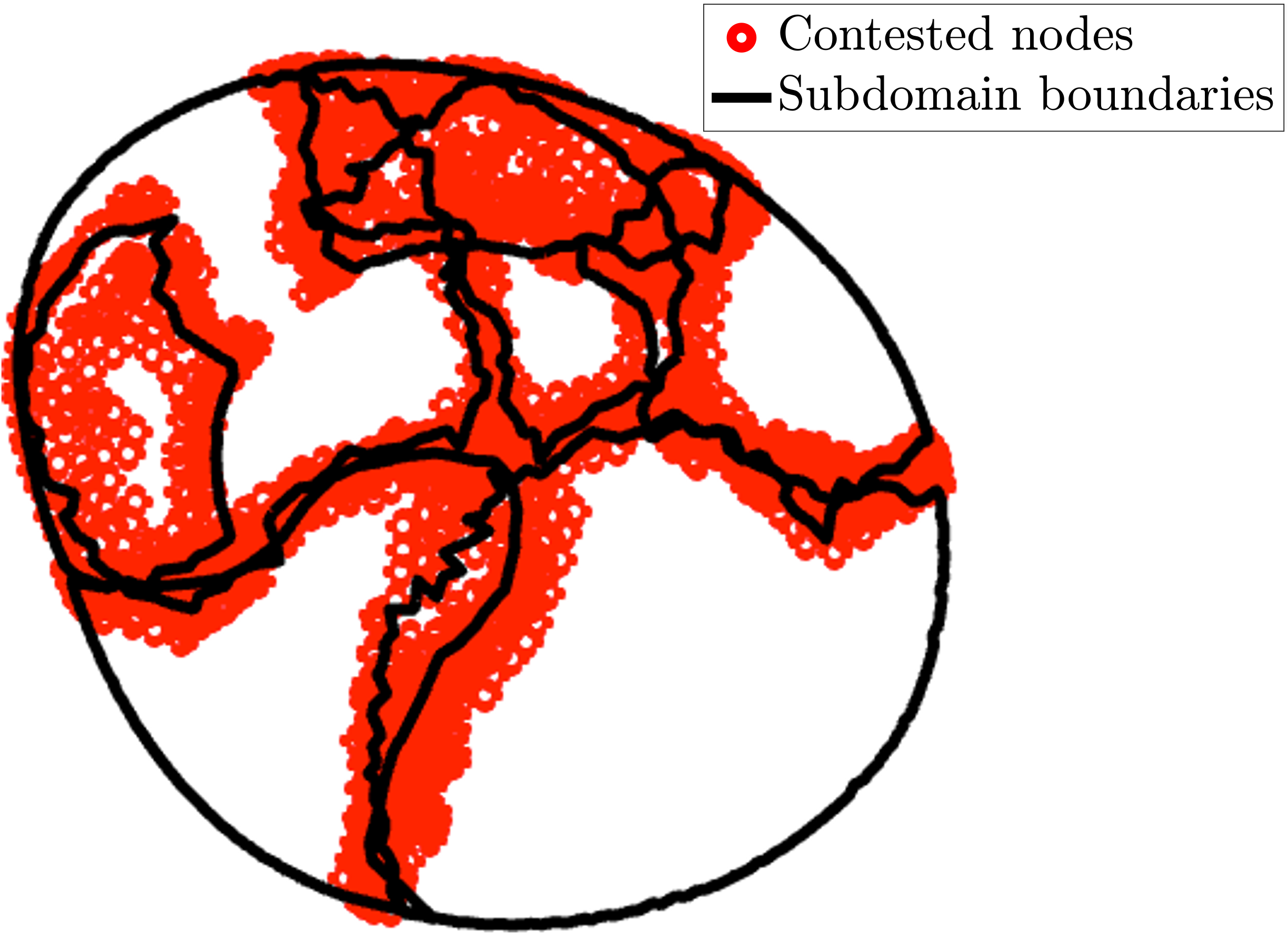
This method of subdomain growth has the flaw that the final subdomain assignment is affected by the order in which the elements are considered. The robustness of the algorithm can be assessed by randomly permuting the list of elements prior to the subdomain assignment. In 1000 samples for the subdivision of $B_{6}$, 88.96 % (15514 of 17440) nodes are always assigned to the same subdomain. Of the 1924 nodes that are not always assigned to the same subdomain, almost all (1914) are assigned to the same subdomain at least 50% of the time and 1178 are assigned to the same subdomain in 80% of the trials. There are 24 nodes that are eligible for assignation to one of 4 subdomains depending on the initial order in which the elements of the mesh are considered. Subdomain 4 has a volume between 2.36 and 3.28 ml (2.85 $\pm$ 0.24 ml); these number of nodes assigned to subdomain 4 is an integer in the interval $[797,841]$. This is the smallest subdomain. Subdomain 5 is the largest with volume in the range 20.21 to 22.93 ml (21.75 $\pm$ 0.66 ml); this subdomain is assigned between 5172 and 5,268 nodes. Subdomain volumes are calculated by taking the computed volume assignations and constructing a concave boundary around each subdomain using the system-specific boundary function (MATLAB R2022b; The MathWorks Inc., Natick, MA, United States) with a shrink factor of 1 . The shrink factor is an optional argument of the boundary function that controls how tightly to the data the boundary is constructed. It lies in the interval $[0,1]$ with a default value of 0.5. As there is some separation between the spatial locations of the nodes that belong to subdomains, the cumulative computed subdomain volume always falls short of the volume of the whole domain. A denser mesh will give a smaller shortfall with the drawback of increased computational time. The correct subdomains are not known a priori, so there is no way to assess the absolute correctness of the grown subdomains. It can be expected that the certainty of the assignations decreases with increasing subdomain count.

As can reasonably be expected, the contested nodes tend to lie on the interface between subdomains as can be seen in Fig. 12.

The final subdivision for $B_{6}$ from the terminal and initial nodes of the terminal branches of the principal pathway are shown in Figs. 13a and 13b, respectively. Subdomain 5 can be seen to be much larger when constructed using an initial node search, rather than a terminal node search. Expected since most of the cyan nodes shown in Fig. 9a are absorbed into the downstream tree from which the subdomain is grown. The optimal selection of nodes from which to search for downstream trees in order to grow subdomains is currently unclear. This is an area that should be investigated in future research.

The final subdivision of the ventricle with the tree $B_{20}$ features more subdomains than that for $B_{6}$. The division with the terminal node search results in a subdomain with 0 volume, where the initial node search results in no subdomains of 0 volume. Given that there is a subdomain of 0 volumes, the assumption that there is a bijective map between the terminal branches of the principal pathway and the subdomains breaks down. In this case, two terminal branches would perfuse a single subdomain. Given this, if the bijective assumption is made, care must be taken when constructing the principal pathway to ensure that there are sufficiently few terminal branches so that no subdomain has 0 volume.

References

- [1] R. H. Haynes. Physical aspects of the mammalian circulatory system. Transactions of the Society of Rheology, 7(1):19–24, 1963.
- [2] R. A. Walsh, J. C. Fang, and V. Fuster, editors. Hurst’s The Heart: Manual of Cardiology. McGraw Hill Medical, New York, NY, thirteenth edition, 2013.
- [3] K. S. Hunter, S. R. Lammers, and R. Shandas. Pulmonary vascular stiffness: measurement, modeling, and implications in normal and hypertensive pulmonary circulations. Comprehensive Physiology, 1(3):1413, 2011.
- [4] M. Leitschuh and A. Chobanian. Vascular changes in hypertension. The Medical clinics of North America, 71(5):827–841, 1987.
- [5] C. M. Akbari and F. W. LoGerfo. Diabetes and peripheral vascular disease. Journal of vascular surgery, 30(2):373–384, 1999.
- [6] M. Lindstrom et al. Global burden of cardiovascular diseases and risks collaboration, 1990-2021. Journal of the American College of Cardiology, 80(25):2372–2425, 2022.
- [7] J. Lee et al. In silico coronary wave intensity analysis: application of an integrated one-dimensional and poromechanical model of cardiac perfusion. Biomechanics and modeling in mechanobiology, 15:1535–1555, 2016.
- [8] L. O. Müller and E. F. Toro. A global multiscale mathematical model for the human circulation with emphasis on the venous system. International journal for numerical methods in biomedical engineering, 30(7):681–725, 2014.
- [9] J. P. Mynard and J. J. Smolich. Influence of anatomical dominance and hypertension on coronary conduit arterial and microcirculatory flow patterns: a multiscale modeling study. American Journal of Physiology-Heart and Circulatory Physiology, 311(1):H11–H23, 2016.
- [10] M. S. Olufsen et al. Rarefaction and blood pressure in systemic and pulmonary arteries. Journal of fluid mechanics, 705:280–305, 2012.
- [11] M. U. Qureshi et al. Numerical simulation of blood flow and pressure drop in the pulmonary arterial and venous circulation. Biomechanics and modeling in mechanobiology, 13(5):1137–1154, 2014.
- [12] M. Zamir and H. Chee. Branching characteristics of human coronary arteries. Canadian journal of physiology and pharmacology, 64(6):661–668, 1986.
- [13] D. A. Nordsletten et al. Structural morphology of renal vasculature. American Journal of Physiology-Heart and Circulatory Physiology, 291(1):H296–H309, 2006.
- [14] M. J. Chambers, M. J. Colebank, M. U. Qureshi, R. Clipp, and M. S. Olufsen. Structural and hemodynamic properties of murine pulmonary arterial networks under hypoxia-induced pulmonary hypertension. Proceedings of the Institution of Mechanical Engineers, Part H: Journal of Engineering in Medicine, 234(11):1312–1329, 2020.
- [15] A. Schuster et al. An isolated perfused pig heart model for the development, validation and translation of novel cardiovascular magnetic resonance techniques. Journal of Cardiovascular Magnetic Resonance, 12(1):1–9, 2010.
- [16] A. Goyal et al. Model-based vasculature extraction from optical fluorescence cryomicrotome images. IEEE transactions on medical imaging, 32(1):56–72, 2012.
- [17] M. Termeer, J. O. Bescós, M. Breeuwer, A. Vilanova, and F. Gerritsen. Patient-specific mappings between myocardial and coronary anatomy. In Dagstuhl Follow-Ups, volume 1, pages 196 – 209. Schloss Dagstuhl-Leibniz-Zentrum fuer Informatik, 2010.
- [18] S. Ham et al. Myocardial territory segmentation on coronary computed tomography angiography images: comparison between projection and non-projection methods in a pig model. Informatics in Medicine Unlocked, 19:100320, 2020.
- [19] J. A. Mackenzie. A 1D model for the pulmonary and coronary circulation accounting for time-varying external pressure. PhD thesis, University of Glasgow, 2021.
- [20] E. R. Hyde et al. Multi-scale parameterisation of a myocardial perfusion model using whole-organ arterial networks. Annals of biomedical engineering, 42(4):797–811, 2014.
- [21] E. Van Bavel and J. A. Spaan. Branching patterns in the porcine coronary arterial tree. estimation of flow heterogeneity. Circulation research, 71(5):1200–1212, 1992.
- [22] J. P. Mynard, D. J. Penny, and J. J. Smolich. Scalability and in vivo validation of a multiscale numerical model of the left coronary circulation. American Journal of Physiology-Heart and Circulatory Physiology, 306(4):H517–H528, 2014.
- [23] M. Termeer et al. Visualization of myocardial perfusion derived from coronary anatomy. IEEE transactions on visualization and computer graphics, 14(6):1595–1602, 2008.
- [24] M. Sinclair et al. Microsphere skimming in the porcine coronary arteries: Implications for flow quantification. Microvascular research, 100:59–70, 2015.
- [25] P. van Horssen et al. Extraction of coronary vascular tree and myocardial perfusion data from stacks of cryomicrotome images. In International Conference on Functional Imaging and Modeling of the Heart, pages 486–494. Springer, 2009.
- [26] J. P. H. M. van den Wijngaard et al. Porcine coronary collateral formation in the absence of a pressure gradient remote of the ischemic border zone. American Journal of Physiology-Heart and Circulatory Physiology, 300(5):H1930–H1937, 2011.
- [27] E. W. Dijkstra. A note on two problems in connexion with graphs. Numerische mathematik, 1(1):269–271, 1959.
- [28] M. J. Chambers. Morphological Properties of Pulmonary Arteries in Control and Hypertensive Mice. PhD thesis, North Carolina State University, 2022.
- [29] O. M. Miller. Notes on cylindrical world map projections. Geographical Review, 32(3):424–430, 1942.
- [30] R. E. Horton. Erosional development of streams and their drainage basins; hydrophysical approach to quantitative morphology. Geological society of America bulletin, 56(3):275–370, 1945.
- [31] A. N. Strahler. Hypsometric (area-altitude) analysis of erosional topography. Geological society of America bulletin, 63(11):1117–1142, 1952.
- [32] A. N. Strahler. Quantitative analysis of watershed geomorphology. Eos, Transactions American Geophysical Union, 38(6):913–920, 1957.
- [33] Z. L. Jiang, G. S. Kassab, and Y. C. Fung. Diameter-defined Strahler system and connectivity matrix of the pulmonary arterial tree. Journal of Applied Physiology, 76(2):882–892, 1994.
- [34] L. O. Schwen and T. Preusser. Analysis and algorithmic generation of hepatic vascular systems. International journal of hepatology, 2012, 2012.
- [35] S. Holcombe. inpolyhedron – are points inside a triangulated volume? MATLAB Central File Exchange, 2016.
- [36] D. C. Manuel et al. Standardized myocardial segmentation and nomenclature for tomographic imaging of the heart. Circulation, 105(4):539–542, 2002.
- [37] M. A. Bartolo et al. Computational framework for the generation of one-dimensional vascular models accounting for uncertainty in networks extracted from medical images. The Journal of Physiology, 602(16):3929–3954, 2024.
- [38] G. S. Kassab, C. A. Rider, N. J. Tang, and Y. C. Fung. Morphometry of pig coronary arterial trees. American Journal of Physiology-Heart and Circulatory Physiology, 265(1):H350–H365, 1993.
- [39] G. S. Kassab, D. H. Lin, and Y. C. Fung. Morphometry of pig coronary venous system. American Journal of Physiology-Heart and Circulatory Physiology, 267(6):H2100–H2113, 1994.
- [40] B. Kaimovitz, Y. Lanir, and G. S. Kassab. A full 3-d reconstruction of the entire porcine coronary vasculature. American Journal of Physiology-Heart and Circulatory Physiology, 299(4):H1064–H1076, 2010.
- [41] B. Kaimovitz, Y. Lanir, and G. S. Kassab. Large-scale 3-d geometric reconstruction of the porcine coronary arterial vasculature based on detailed anatomical data. Annals of biomedical engineering, 33:1517–1535, 2005.
- [42] H. Schröder, N. Moser, and S. Huggenberger. Rodent basic neuroanatomy/coverings of the cns/cerebrospinal fluid system. Neuroanatomy of the Mouse: An Introduction, pages 27–44, 2020.
- [43] R. L. Shreve. Statistical law of stream numbers. The Journal of Geology, 74(1):17–37, 1966.