Spectral Functions of Gauge Theories with Banks-Zaks Fixed Points

We are interested in four-dimensional Yang-Mills theories with gauge group $SU(N_{c})$ coupled to $N_{f}$ massless Dirac fermions $\psi$ in the fundamental representation. Modulo gauge-fixing and ghost terms, the perturbatively renormalisable Lagrangian is given by

$\displaystyle L$

$\displaystyle=-\frac{1}{2}\text{Tr}\!\left(F_{\mu\nu}F^{\mu\nu}\right)+\text{Tr}\!\left(\bar{\psi}i\not{D}\psi\right),$

(1)

where $F_{\mu\nu}$ is the field strength of the gauge bosons, and the trace runs over the colour and flavour indices. The theory has a global $U(N_{f})$ flavour symmetry and is otherwise characterised by the gauge and matter field multiplicities, and by the gauge coupling $g$, which we scale with a perturbative loop factor

$\displaystyle a=g^{2}/(16\pi^{2})\,.$

(2)

The dependence of the gauge coupling on the energy scale $\mu$ is expressed via the $\beta$-function $\beta(a)\equiv\mu^{2}{\differential a(\mu^{2})}/{\differential\mu^{2}}$. In perturbation theory, it is given by

$\displaystyle\beta(a)=\sum_{n=1}\beta_{n}\,a^{n+1}\,,$

(3)

with loop coefficients $\beta_{n}$ known up to five-loop order in the $\overline{\textrm{MS}}$ scheme Herzog:2017ohr.

Free or interacting renormalisation group fixed points with $\beta(a_{*})=0$ are of particular interest Polchinski:1987dy, the reason being that scale-invariance for any relativistic and unitary four-dimensional theory that remains perturbative in the UV or IR asymptotes into a conformal field theory Komargodski:2011vj; Komargodski:2011xv; Luty:2012ww. The theory eq. 1 always displays a free Gaussian fixed point $a_{*}=0$. For sufficiently few matter fields, the one-loop coefficient $\beta_{1}$ is negative leading to asymptotic freedom such as in QCD Gross:1973id; Politzer:1973fx. Conversely, adding too many matter fields implies that asymptotic freedom is lost and the theory becomes IR free such as in QED.

The competition of gauge and matter field fluctuations may also lead to interacting quantum fixed points $(a_{*}>0)$. At weak coupling, interacting fixed points are either of the Banks-Zaks (BZ) or the gauge-Yukawa (GY) type Bond:2016dvk; Bond:2018oco. BZ fixed points Belavin:1974gu; Caswell:1974gg; Banks:1981nn are always IR in any quantum field theory Bond:2016dvk, while fixed points involving Yukawa interactions may be either IR or UV Bond:2016dvk; Bond:2018oco, see Litim:2014uca; Litim:2015iea; Bond:2016dvk; Bond:2017wut; Bond:2017tbw; Bond:2017lnq; Bond:2017suy; Bond:2019npq. It is also well-established that conformal windows with BZ or GY fixed points exist at strong coupling, see e.g. Gies:2005as; Dietrich:2006cm; Jarvinen:2011qe; Kusafuka:2011fd; Alvares:2012kr; DeGrand:2015zxa; Gukov:2016tnp; Simmons-Duffin:2016gjk; Poland:2018epd; Ryttov:2016ner; Ryttov:2017lkz; Kuipers:2018lux; Hasenfratz:2018wpq; Fodor:2018uih; Antipin:2018asc; Hasenfratz:2019dpr; DiPietro:2020jne; Kim:2020yvr; Bond:2021tgu; Bond:2022xvr. For a recent conjecture of a BZ phase with spontaneously broken scale symmetry, see DelDebbio:2021xwu.

Much less is known about the fixed points outside the BZ or GY conformal windows. In pure Yang-Mills theory, it has been suggested that its IR limit relates to a non-perturbative fixed point, e.g. Aguilar:2002tc; Gies:2002af; Pawlowski:2003hq. In a different vein, it has also been speculated that a new strongly interacting UV fixed points may arise in the many fermion limit PalanquesMestre:1983zy; Gracey:1996he; Holdom:2010qs, though the viability for this has been called into question as of late Martin:2000cr; Ryttov:2019aux; Alanne:2019vuk; Leino:2019qwk; Dondi:2019ivp; Dondi:2020qfj; Bond:2021tgu.

In this work, we focus on settings with a BZ fixed point and exploit results from perturbation theory up to five loops and suitable resummations thereof.

Our starting point is a regime with a BZ fixed point Belavin:1974gu; Caswell:1974gg; Banks:1981nn, which, furthermore, is under strict perturbative control. If so, the running gauge coupling remains small along the entire renormalisation group (RG) trajectory interpolating between asymptotic freedom in the UV and a perturbatively controlled BZ fixed point in the IR. Most notably perturbative methods are sufficient to analyse the properties of the theory.

In this spirit, we notice that the $\beta$-function eq. 3 features a non-trivial BZ fixed point, which takes the form

$\displaystyle a_{*}=-\frac{\beta_{1}}{\beta_{2}}+\order{\beta_1^2}$

(4)

to the leading orders in perturbation theory. The one- and two-loop coefficients are given by

	$\displaystyle\beta_{1}$	$\displaystyle=-\frac{2N_{c}}{3}\varepsilon\,,$
	$\displaystyle\beta_{2}$	$\displaystyle=\frac{25N_{c}^{2}-11}{2}+\frac{3-13N_{c}^{2}}{3}\varepsilon\,.$		(5)

Here, we introduced the Veneziano parameter $\varepsilon$

$\displaystyle\varepsilon=\frac{11}{2}-\frac{N_{f}}{N_{c}}\,,$

(6)

to replace the free parameters $(N_{c},N_{f})$ by $(N_{c},\varepsilon)$. The parameter eq. 6 may take values between $[-\infty,\frac{11}{2}]$. For $\varepsilon>0$, the theory is asymptotically free, corresponding to $N_{f}<\frac{11}{2}N_{c}$. Further, the one loop gauge coefficient is parametrically small provided that

$\displaystyle 0<\varepsilon\ll 1\,.$

(7)

Consequently, interacting fixed points in the regime eq. 7 are under strict perturbative control Banks:1981nn; Bond:2019npq.

The fixed point eq. 4 stems from a cancellation between the one-loop term and the remainder of the $\beta$-function, starting with the two-loop coefficient. Such a cancellation leads to a reliable fixed point within perturbation theory if $\beta_{1}/\beta_{2}$ in eq. 4 is parametrically small. This is precisely the case when $\varepsilon\ll 1$, and provided that the two-loop term $\beta_{2}$ remains of order unity and positive. The latter holds true in general: for any $4d$ quantum gauge theory coupled to matter with a parametrically small one loop coefficient $\beta_{1}$, the two-loop coefficient $\beta_{2}$ is of order unity, and strictly positive Bond:2016dvk. Hence, BZ fixed points are invariably IR and never UV.

A regime with arbitrarily small $\varepsilon$ can always be achieved in the large-$N$ Veneziano limit where $N_{c},N_{f}\to\infty$ with $N_{f}/N_{c}$ fixed, and where the parameter eq. 6 becomes continuous, also reducing the number of free parameters to one. In this work, we follow two strategies to determine fixed points: Firstly, we use the perturbative loop expansion to determine fixed points from order to order. This provides the fixed point as a rational function of $\varepsilon$, and will mostly be used when $N_{c},N_{f}$ are finite. Alternatively, we may determine the fixed point as a strict power series in $\varepsilon$. The latter mixes contributions from different loop orders owing to the fact that loop coefficients $\beta_{i}/(N_{c})^{i}$ contain terms of different order in $\varepsilon$, see section II.2. In the Veneziano limit, this is sometimes referred to as the conformal expansion.

Beginning with the loop expansion and neglecting three- and higher-loop corrections, we can find an analytical solution for the running coupling to study its properties in the complex plane. At two-loop order, the value for the BZ fixed point reads

$\displaystyle a_{*}=\frac{4\varepsilon}{N_{c}(75-26\varepsilon)-\tfrac{6}{N_{c}}\left(\frac{11}{2}-\varepsilon\right)}\,.$

(8)

Further, its universal scaling exponent

$\displaystyle\theta=\left.\frac{\partial\beta_{a}}{\partial a}\right|_{a=a_{*}},$

(9)

is given by

$\displaystyle\theta=\frac{8}{3}\frac{\varepsilon^{2}}{\left(75-26\varepsilon\right)-\tfrac{6}{N_{c}^{2}}\left(\frac{11}{2}-\varepsilon\right)}\,,$

(10)

at two-loop accuracy. The corresponding RG trajectory for the running gauge coupling that connects the asymptotically free UV fixed point with the BZ fixed point in the IR, as shown in fig. 1, can be found analytically (see appendix A). It reads Corless:1996zz; Gardi:1998qr

$\displaystyle a(\mu^{2})=\frac{a_{*}}{1+W_{0}(z)}\,,$

(11)

in terms of the principal branch of the $W$-Lambert function, with

$\displaystyle z(\mu^{2})$

$\displaystyle=\omega_{0}e^{\omega_{0}}\left(\frac{\mu^{2}}{\mu_{0}^{2}}\right)^{\!\theta}\,,$

$\displaystyle\omega_{0}$

$\displaystyle=\frac{a_{*}-a_{0}}{a_{0}}\,,$

(12)

and initial condition $a(\mu_{0}^{2})=a_{0}$. As such, the expressions eqs. 8, 10, 11 and 12 are the two-loop results for the BZ fixed point and the running coupling for all scales.

The gauge coupling interpolates between asymptotic freedom in the UV and the Banks-Zaks fixed point in the IR. The transition between the two scaling regimes is characterised by an RG invariant cross-over scale $\Lambda_{c}$, indicated in fig. 1. It can be written as

$$\Lambda_{c}=\mu\cdot\exp(\frac{1}{\beta_1\,\delta\alpha(\mu)})\,,$$

(13)

where $0<\delta\alpha(\mu)\ll\alpha_{*}$ denotes the initial deviation of the gauge coupling from its free UV fixed point at the high scale $\mu$, while $\beta_{1}<0$ denotes the one-loop gauge coefficient, see section II.2. It is readily confirmed that $\mathrm{d}\Lambda_{c}/\mathrm{d}\ln\mu=0$. Notice that the expression eq. 13 is parametrically the same as for any asymptotically free gauge theory and coincides with the definition for $\Lambda_{\rm QCD}$ in perturbative QCD, as it must, because the UV initial condition $\delta\alpha$ does not know that the theory achieves an interacting fixed point rather than confinement in the IR.

Alternatively, we can perform a conformal expansion organised in powers of the Veneziano parameter $\varepsilon$. We expand the BZ fixed point and its critical exponent up to the appropriate power of $\varepsilon$. From two-loop perturbation theory, we can obtain leading order expressions in $\varepsilon$ for the BZ fixed point

$\displaystyle N_{c}a_{*}=\frac{4}{75}\varepsilon+\mathcal{O}\!\left(\varepsilon^{2},\frac{1}{N_{c}^{2}}\right),$

(14)

as well as its eigenvalue

$\displaystyle\theta=\frac{8}{225}\varepsilon^{2}+\mathcal{O}\!\left(\varepsilon^{3},\frac{1}{N_{c}}\right).$

(15)

Higher-order expressions for the fixed point and the scaling exponent up to five loop order in the Veneziano limit are given in appendix B. Inserted into eq. 11 leads to the running coupling at leading order in the Veneziano expansion.

For small $\varepsilon\ll 1$, the difference between loop expansion and the Veneziano expansion is parametrically small. For larger values of $\varepsilon$, there is a quantitative difference between the loop expansion and the Veneziano expansion due to the fact that loop coefficients may contain different orders in $\varepsilon$. In this work, we display results in both expansions. In the conformal expansion, we restrict ourselves to small $\varepsilon$ and work exclusively in the $N_{c}\to\infty$ limit. In the loop expansion, we also explore larger values of $\varepsilon$ as well as small values of $N_{c}$.

We now discuss the properties of the running coupling in the complex $\mu^{2}/\mu_{0}^{2}$ plane. While $a$ is uniquely defined for $\mu^{2}/\mu_{0}^{2}>0$, uniqueness is lost in the complex plane provided there are branch cuts. There are two sources of branching points:

• (i)

  the branching point at $\mu^{2}/\mu_{0}^{2}=0$ originating from the power law in the definition of $z$ in eq. 12,

• (ii)

  further branching points originating through the $W$-Lambert function.

The branching point of the first type (i) is always present and continues along $\mu^{2}/\mu_{0}^{2}<0$ until $-\infty$. This branch cut is important for the physics as its discontinuity later results in the spectral functions of the fields.

In contrast to that, the branching points of the second type (ii) may be absent or present including in larger numbers, depending on the values for $\varepsilon$ and $N_{c}$. As we will see, these types of branching points spoil the existence of a standard KL spectral representation.

The principal branch of the $W$-Lambert function $W_{0}(z)$ has its branch cut starting at $z=-1/e$ and is chosen to continue along the negative $z$ axis towards $z=-\infty$. Thus, to obtain the branch cut of $W_{0}(z)$ we must have

$\displaystyle z(\mu^{2})<-\frac{1}{e}\,.$

(16)

In order for this equation to have a solution, the phase of $\mu^{2}/\mu_{0}^{2}$ must be given by

$\displaystyle\varphi(\mu^{2}/\mu_{0}^{2})=-\frac{\pi}{\theta}(2n+1)\,,$

(17)

with $n$ an integer and $\theta$ the eigenvalue of the BZ fixed point given in eq. 10 and eq. 15. Using the principal branch, only those solutions in eq. 17 exist which contain a phase $\varphi$ with $-\pi<\varphi\leq\pi$. This leads us to the requirement

$\displaystyle-\frac{1}{|\theta|}<2n+1\leq\frac{1}{|\theta|}\,,$

(18)

which means the number of branching points originating from the $W$-Lambert function is given by twice the amount of odd numbers less than $|\theta|$. For the total number of branch cuts, this means

$\displaystyle\#\text{bp}=1+2\left\lfloor\frac{\left|\theta\right|+1}{2}\right\rfloor.$

(19)

The existence of non-analyticities for $|\theta|>1$ was first noticed in Gardi:1998ch. In fig. 2, we show the resulting number of branching points as a function of $\varepsilon$ using the two-loop expression of the BZ eigenvalue eq. 10. We observe a single branch cut at $\mu^{2}/\mu^{2}_{0}=0$ at weak and moderate coupling ($0<\varepsilon<\varepsilon_{\rm branch\,cut}$), with

$\displaystyle\varepsilon_{\rm branch\,cut}=\left\{\begin{array}[]{lcr}2.2723&{\rm for}&N_{c}=3\,,\\[4.30554pt] 2.32850&{\rm for}&1/N_{c}=0\,.\end{array}\right.$

At stronger coupling ($\varepsilon_{\text{branch cut}}<\varepsilon<\varepsilon_{\rm max}$), and beyond the threshold $\varepsilon_{\text{branch cut}}$, their number rapidly proliferates into many more branching points with increasing $\varepsilon$. Their number diverges just when the fixed point ceases to exist $(\varepsilon=\varepsilon_{\rm max})$, with

$\displaystyle\varepsilon_{\rm max}=\left\{\begin{array}[]{lcr}2.8158&{\rm for}&N_{c}=3\,,\\[4.30554pt] 2.8846&{\rm for}&1/N_{c}=0\,,\end{array}\right.$

at two-loop accuracy.

The presence of branch cuts signifies that the analytic continuation of the running gauge coupling into the complex plane is not unique, simply because the location of branch cuts is ambiguous. In fact, even the number of branching points may become ambiguous due to e.g. the properties of the $W$-Lambert function. In fig. 3, we illustrate this ambiguity at two-loop, using $\varepsilon=2.7$. In the standard prescription in the left panel of fig. 3, we follow eq. 11 and observe in total five branching points, four of which are obtained from the $W$-Lambert function. The plot in the right panel of fig. 3 instead assumes the running coupling to be given by

$\displaystyle a(\mu^{2})=\frac{a_{*}}{1+W_{i}(z)}\,,$

(24)

with

$\displaystyle i=\begin{cases}-2&\phantom{\text{for}\;\varphi(\mu^{2}/\mu_{0}^{2})}<-3\frac{\pi}{\theta}\\[4.30554pt] -1&\phantom{\text{for}\;\varphi(\mu^{2}/\mu_{0}^{2})}<-1\frac{\pi}{\theta}\\[4.30554pt] \ \ 0&\text{for}\;\varphi(\mu^{2}/\mu_{0}^{2})<\ \ 1\frac{\pi}{\theta}\\[4.30554pt] \ \ 1&\phantom{\text{for}\;\varphi(\mu^{2}/\mu_{0}^{2})}<\ \ 3\frac{\pi}{\theta}\\[4.30554pt] \ \ 2&\phantom{\text{for}\;\varphi(\mu^{2}/\mu_{0}^{2})}>\ \ 3\frac{\pi}{\theta}\end{cases}\,.$

(25)

Since only $W_{0}(z)$ has a branching point at $z=-1/e$ and all other branches at $z=0$, two branching points have moved due to this prescription to the origin and their branch cuts go along the negative axis towards $-\infty$. Thus, the presence of additional branch cuts turns out to make the running coupling in the complex plane ambiguous.

At this point, we want to compute the propagator for all momenta using perturbative methods. We consider all species of particles included in the theory, i.e., gluons, quarks, and ghosts. Starting from corresponding two-point functions, we follow, e.g., Chetyrkin:2000dq and define

	$\displaystyle D_{\mu\nu}^{ab}(p)$	$\displaystyle\equiv i\int\!\differential^{d}x\,e^{ipx}\langle TA_{\mu}^{a}(x)A_{\nu}^{b}(0)\rangle\,,$
	$\displaystyle\Delta^{ab}(p)$	$\displaystyle\equiv i\int\!\differential^{d}x\,e^{ipx}\langle Tc^{a}(x)\bar{c}^{b}(0)\rangle\,,$
	$\displaystyle S_{ij}(p)$	$\displaystyle\equiv i\int\!\differential^{d}x\,e^{ipx}\langle T\psi_{i}(x)\bar{\psi}_{j}(0)\rangle\,.$		(26)

The tensor structures of the propagators follow from general arguments such as Ward identities with only the self energies being undetermined,

	$\displaystyle D_{\mu\nu}^{ab}(p)$	$\displaystyle=\frac{\delta^{ab}}{-p^{2}}\left[\left(-g_{\mu\nu}+\frac{p_{\mu}p_{\nu}}{p^{2}}\right)\frac{1}{1+\Pi_{A}(p^{2},\mu^{2})}-\xi\frac{p_{\mu}p_{\nu}}{p^{2}}\right],$
	$\displaystyle\Delta^{ab}(p)$	$\displaystyle=\frac{\delta^{ab}}{-p^{2}}\frac{1}{1+\Pi_{c}(p^{2},\mu^{2})}\,,$
	$\displaystyle S_{ij}(p)$	$\displaystyle=\frac{\delta^{ij}}{-p^{2}}\frac{\not{p}}{1+\Pi_{\psi}(p^{2},\mu^{2})}\,.$		(27)

Perturbative results for the self-energies $\Pi_{\phi}$ for all the propagators $\phi\in\{A,c,\psi\}$ have been obtained in Chetyrkin:2000dq; Ruijl:2017eht. These contain logarithmic contributions of the form $\log(-p^2/\mu^2)$ which diverge in the UV as well as in the IR. These large logarithms lead to a breakdown of the perturbative expansion and it is required to resum them in order to obtain the correct large and small momentum behaviour.

A practical tool to resum logarithmic contributions lies in the perturbative renormalisation group for $n$-point functions. It stems from the property of a bare $n$-point function being independent of the renormalisation scale $\mu^{2}$. We apply it here to the scalar parts of the propagators defined with

$\displaystyle G_{\phi}(p^{2},\mu^{2})$

$\displaystyle=\frac{1}{-p^{2}}\frac{1}{1+\Pi_{\phi}(p^{2},\mu^{2})}\,.$

(28)

For the bare propagators $G_{\phi,b}$, the independence of $\mu^{2}$ implies

$\displaystyle\mu^{2}\frac{\differential}{\differential\mu^{2}}G_{\phi,b}=\mu^{2}\frac{\differential}{\differential\mu^{2}}\left(Z_{\phi}\,G_{\phi}\right)=0\,.$

(29)

Here, we denote the renormalised propagator as $G_{\phi}$ and $Z_{\phi}$ is the renormalisation constant of the field $\phi$. The perturbative propagator depends on the renormalisation scale only through the running coupling and the logarithmic terms that we want to resum. Therefore, we obtain the Callan-Symanzik (CS) equation

$\displaystyle\left(\mu^{2}\frac{\partial}{\partial\mu^{2}}+\beta(a)\frac{\partial}{\partial a}-\gamma_{\phi}\right)G_{\phi}=0\,,$

(30)

with the anomalous dimension defined by

$\displaystyle\gamma_{\phi}=-\frac{1}{Z_{\phi}}\frac{\differential Z_{\phi}}{\differential\log\mu^{2}}\,.$

(31)

Solving eq. 30 results in the general form of the propagator up to an integration constant. This integration constant can be obtained from the perturbative result at the point where the logarithmic corrections vanish, i.e. at $-p^{2}=\mu^{2}$.

To solve eq. 30 we first note that

$\displaystyle G_{\phi}(a,p^{2},\mu^{2})=\frac{f_{\phi}(a,p^{2}/\mu^{2})}{p^{2}}\,,$

(32)

with some function $f_{\phi}$ that only depends on the ratio $p^{2}/\mu^{2}$. This allows us to trade $\mu^{2}$-derivatives for $p^{2}$-derivatives,

$\displaystyle\left(-p^{2}\frac{\partial}{\partial p^{2}}+\beta(a)\frac{\partial}{\partial a}-\gamma_{\phi}-1\right)G_{\phi}(a,p^{2},\mu^{2})=0\,.$

(33)

This differential equation can be solved by the method of characteristics. To that end, we introduce a new momentum dependent running coupling $\bar{a}(-p^{2})$

$\displaystyle\int_{a}^{\bar{a}}\!\frac{\mathrm{d}a^{\prime}}{\beta(a^{\prime})}=\int_{\mu^{2}}^{-p^{2}}\!\frac{\mathrm{d}\bar{p}^{2}}{\bar{p}^{2}}\,.$

(34)

The two-loop solution for $\bar{a}$ is given by the solution for $a$ upon the replacement of $\mu^{2}$ by $-p^{2}$ and $\mu_{0}^{2}$ by $\mu^{2}$,.

$\displaystyle\bar{a}(-p^{2})=\frac{a_{*}}{1+W_{0}(\bar{z})}\,,$

(35)

with

$\displaystyle\bar{z}=\left(\frac{a_{*}}{a}-1\right)e^{a_{*}/a-1}\left(\frac{-p^{2}}{\mu^{2}}\right)^{\!\theta}\,.$

(36)

This allows the elimination of the variable $p^{2}$ in favour of $\bar{a}$. The CS equation for $G_{\phi}(\bar{a},a,\mu^{2})$ then takes the form of an ordinary first-order differential equation

$\displaystyle\left(\beta(a)\frac{\partial}{\partial a}-\gamma_{\phi}-1\right)G_{\phi}=0\,.$

(37)

Its solution $G_{\phi}(\bar{a},a,\mu^{2})$ is given by

$\displaystyle G_{\phi}$

$\displaystyle=\frac{\hat{C}_{\phi}(\bar{a},\mu^{2})}{-p^{2}}\exp( - \int_{a}^{\bar{a}} \!\frac{\text{d} a'}{\beta(a')} \, \gamma_\phi(a') )\,,$

(38)

with $\hat{C}_{\phi}(\bar{a},\mu^{2})$ an integration constant independent of $a$. At two loop accuracy, and writing $\gamma_{\phi}(a)=\gamma_{\phi}^{(1)}a+{\cal O}(a^{2})$, the integral in eq. 38 is given by

$\displaystyle\int_{a}^{\bar{a}}\!\frac{\text{d}a^{\prime}}{\beta(a^{\prime})}\,\gamma_{\phi}(a^{\prime})$

$\displaystyle=\frac{\gamma_{\phi}^{(1)}}{\beta_{1}}\log\frac{\bar{a}}{a}+\frac{\gamma_{\phi}(a_{*})}{\theta}\log\frac{\bar{a}-a_{*}}{a-a_{*}}.$

(39)

The only remaining task is the determination of the integration constant $\hat{C}_{\phi}(\bar{a},\mu^{2})$. This can be obtained by comparing to the perturbative two-loop result at $p^{2}=-\mu^{2}$, leading to

$\displaystyle\hat{C}_{\phi}(\bar{a},\mu^{2})=-\frac{\mathcal{N}_{\phi}}{1+\Pi_{\phi}^{(1)}\bar{a}+\Pi_{\phi}^{(2)}\bar{a}^{2}}\,,$

(40)

where the coefficients $\Pi_{\phi}^{(i)}$ arise from a series expansion of the self energies at $p^{2}=-\mu^{2}$, namely

$\displaystyle\Pi_{\phi}(p^{2}=-\mu^{2})=\Pi_{\phi}^{(1)}a+\Pi_{\phi}^{(2)}a^{2}+\ldots\,.$

(41)

We have included an overall normalisation factor $\mathcal{N}_{\phi}$, which originates from the freedom to rescale wave-function renormalisation $Z_{\phi}$ in eq. 29. The coefficients $\Pi_{\phi}^{(i)}$ have been computed in Chetyrkin:2000dq; Ruijl:2017eht up to four-loop order. The final result for the CS resummed two-loop propagator is

$\displaystyle G_{\phi}$

$\displaystyle=\frac{1}{p^{2}}\frac{\mathcal{N}_{\phi}}{1+\Pi_{\phi}^{(1)}\bar{a}+\Pi_{\phi}^{(2)}\bar{a}^{2}}\left(\frac{a}{\bar{a}}\right)^{\!\gamma_{\phi}^{(1)}/\beta_{1}}\left(\frac{a-a_{*}}{\bar{a}-a_{*}}\right)^{\!\gamma_{\phi}(a_{*})/\theta}\!.$

(42)

From this expression, we find the UV behaviour at the Gaussian fixed point and the IR behaviour at the BZ fixed point. Close to the Gaussian fixed point, the term $(a/\bar{a})^{\gamma_{\phi}^{(1)}/\beta_{1}}$ in eq. 42 dominates, while in the IR, the last term in eq. 42 corresponding to the BZ fixed point produces an IR behaviour characterised by the anomalous dimension evaluated at the fixed point and its critical exponent. Using the asymptotics of the running coupling in eq. 117, the explicit large and small momentum asymptotics of the propagator are

$\displaystyle G_{\phi}=\left\{\begin{array}[]{ll}\frac{N^{\text{UV}}_{\phi}}{p^{2}}\left[\log( - \frac{p^2}{\mu^2})\right]^{\gamma^{(1)}_{\phi}/\beta_{1}}&\text{for }\left|p^{2}\right|\to\infty\,,\\[8.61108pt] \frac{N^{\text{IR}}_{\phi}}{p^{2}}\left(-\frac{p^{2}}{\mu^{2}}\right)^{-\gamma_{\phi}(a_{*})}&\text{for }\left|p^{2}\right|\to 0\,.\end{array}\right.$

The large momentum asymptote is well known and relates to the Oehme-Zimmermann superconvergence relation Oehme:1979ai; Oehme:1979bj; Oehme:1990kd. Note that the critical exponent in eq. 42 cancels against the critical exponent from the power law of the running coupling in the IR such that the leading power in the IR limit of section II.4 is independent of the critical exponent. The normalisation factors $N^{\text{IR}}_{\phi}$ and $N^{\text{UV}}_{\phi}$ in section II.4 read

	$\displaystyle N^{\text{IR}}_{\phi}$	$\displaystyle=\mathcal{N}_{\phi}\frac{e^{\left(1-a_{*}/a\right)\gamma_{\phi}(a_{*})/\theta}}{1+\Pi_{\phi}^{(1)}a_{*}+\Pi_{\phi}^{(2)}a_{*}^{2}}\left(\frac{a}{a_{*}}\right)^{\gamma_{\phi}^{(1)}/\beta_{1}+\gamma_{\phi}(a_{*})/\theta},$
	$\displaystyle N^{\text{UV}}_{\phi}$	$\displaystyle=\mathcal{N}_{\phi}\left(-\beta_{1}a\right)^{\gamma_{\phi}^{(1)}/\beta_{1}}\left(\frac{a_{*}-a}{a_{*}}\right)^{\gamma_{\phi}(a_{*})/\theta}.$		(45)

and we choose the normalisation factor $\mathcal{N}_{\phi}$ such that $N^{\text{UV}}_{\phi}=1$. This choice will later ensure that the spectral function is properly normalised.

The CS-resummed gluon propagator $G_{A}(p^{2})$ at two-loop is shown in fig. 4 in the Veneziano limit ($\varepsilon=\frac{1}{2}$, $\xi=1$). We observe that the propagator quickly approaches its asymptotic limits given by section II.4, with a smooth crossover regime in between.¹¹ 1 Here and below, we display propagators and spectral functions as functions of $(p^{2})^{\theta}$, which arises naturally in the argument of the $W$-Lambert function, eqs. 35 and 36. This choice naturally accounts for the parametrically slow running of the gauge coupling. The range shown in fig. 4 corresponds to scales between $p^{2}=\mathcal{O}(10^{-300})$ and $p^{2}=\mathcal{O}(10^{300})$. For smaller $\varepsilon$, the range quickly becomes larger.

Next, we need to understand the analytical properties of propagators in the plane of complexified momenta $p^{2}$. In particular, we need to understand whether the propagator admits branch cuts or poles. There are three possible origins for the latter. These are

• (i)

  branch cuts from the running coupling $\bar{a}$,

• (ii)

  branch cuts from the explicit power laws in eq. 42,

• (iii)

  poles from the self-energy term in eq. 42.

Next, we discuss the different cases one by one.

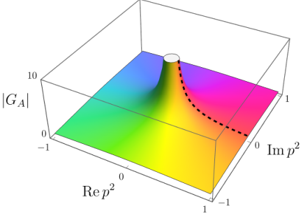
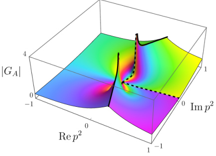
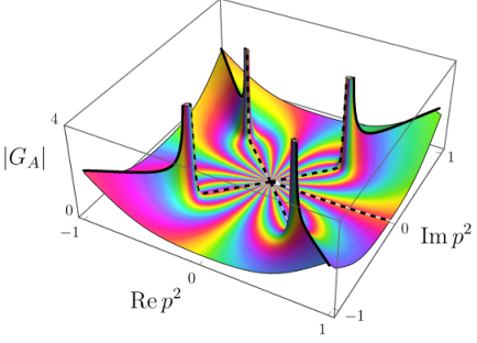
Case (i). Branch cuts originating from the running coupling $\bar{a}$ have been discussed in section II.3. To apply these findings to the propagator, we replace $\mu^{2}\rightarrow-p^{2}$ and $\mu_{0}^{2}\rightarrow\mu^{2}$ as well as $a\rightarrow\bar{a}$ and $a\rightarrow a_{0}$. Then, the running coupling leads to two kinds of branch cuts in the propagator:

• a)

  The branch cut at $p^{2}/\mu^{2}<0$ originating from the power law in the definition of $\bar{z}$.

• b)

  Branch cuts for $p^{2}/\mu^{2}$ such that $\bar{z}<-1/e$, which originate from the branch cuts of $W_{0}(\bar{z})$.

As discussed in section II.3, the branch cut a) is important for the physics. In turn, branch cuts of the type b) are “dangerous” in that they spoil the existence of a standard KL spectral representation.

Case (ii). The explicit power laws in eq. 42 lead to branch cuts when

$\displaystyle\frac{a}{\bar{a}}$

$\displaystyle<0\,,$

or

$\displaystyle\frac{a-a_{*}}{\bar{a}-a_{*}}$

$\displaystyle<0\,.$

(46)

Since $a>0$, the former is reached only if $\bar{a}<0$, i.e., $W_{0}(\bar{z})<-1$. There are no values $\bar{z}$ where this equation is fulfilled if the principal branch of the W-Lambert function is used. Instead, the W-Lambert function only takes these values in the branch $W_{-1}(\bar{z})$ for $-1/e<\bar{z}<0$. Hence, if we stick to the definition eq. 11 in the complex plane, this does not play a role.

The second condition in eq. 46 can only be fulfilled if

$\displaystyle\bar{a}$

$\displaystyle>a_{*}\,,$

i.e.

$\displaystyle-1$

$\displaystyle<W_{0}(\bar{z})<0\,.$

(47)

These values are reached in the principal branch if

$\displaystyle-\frac{1}{e}<\bar{z}<0\,.$

(48)

Note that the phase for $\bar{z}$ where these branch cuts are reached is the same as for the branch cuts originating from the $W$-Lambert function, only the required absolute value of $\bar{z}$ is different, see eq. 16. Thus, the branch cuts originating from the explicit power laws in eq. 42 extend the branch cuts originating from the $W$-Lambert function. Combining these two sources of the branch cuts, we obtain branch cuts starting at $p^{2}=0$ and reaching up to $p^{2}=\infty$, with the complex phase of these cuts given by eq. 17.

As discussed in section II.3 this means that for small values for $\varepsilon$ only the standard branch cut at $p^{2}>0$ remains. On the other hand, for larger values of $\varepsilon$ we have inevitably additional branch cuts in the complex plane, leading to a propagator which is only analytic in separated and disconnected regions of the complex plane.

Case (iii). A last source of non-analyticities are potential poles from self-energy corrections. Poles arise whenever the denominator of eq. 40 vanishes in the complex plane. If they exist, and depending on their location in the complex plane, they correspond to either stable or unstable physical (bound) states, or to stable or unstable (unphysical) tachyonic states.

For sufficiently small $\varepsilon\rightarrow 0$, we can strictly rule out the existence of self-energy poles based on the following observation: A zero in the self energies can only arise if the coupling in the complex plane becomes of order unity. On the real axis, the coupling is bounded by the BZ fixed point $a_{*}$, which becomes infinitesimally small in this limit. Hence, in the complex plane, the coupling can only become of order unity if the denominator in eq. 35 becomes sufficiently small, which only happens at the branching point of the coupling. However, since this branching point is only reached for sufficiently large $\varepsilon$ (e.g. fig. 2), we conclude that there are no poles from the self energies for $\varepsilon\rightarrow 0$. For larger $\varepsilon$, the reasoning does not apply and we investigate the poles from eq. 40 numerically below, and separately for gluons, fermions, and ghosts.

Our findings are illustrated in fig. 5 where we show the gluon propagator in the complex plane for different values of $\varepsilon$. Depending on the value of $\varepsilon$ we observe one or several branch cuts. Additional branch cuts beyond the standard one come in pairs symmetric about the real axis. The power-law branch cuts (dashed) and the $W$-Lamber branch cuts (solid) align and are connected at the branching point where the coupling, and therefore the propagator, diverges. It follows from our previous discussion of branch cuts of running couplings in the complexified $\mu^{2}$ plane that branch cuts of propagators in the complexified $p^{2}$ plane also imply ambiguities. Similarly, choosing the branch cuts appropriately may lead to the disappearance of some of them.

In our setting, the existence of a KL representation cannot be taken for granted, given that neither gluons nor quarks or ghosts qualify as physical asymptotic states. Still, we are interested in conditions under which their propagators can, nevertheless, be represented by a KL spectral function. A first such condition is that propagators only have a single branch cut on the positive real axis, and are analytic otherwise. At two-loop, we know that this holds for $\varepsilon<\varepsilon_{\rm branch\,cut}$, see section II.3. For $\varepsilon>\varepsilon_{\rm branch\,cut}$ this is spoiled by the existence of additional branch cuts arising from the running coupling eq. 19. The standard KL representation is violated, and a spectral representation would need to be modified, see for example Horak:2022myj for a respective generalisation.

For the single branch cut, we need to check that the spectral integral is convergent. For this we integrate the propagator divided by $p^{2}-\lambda^{2}$ along the keyhole integration contour shown in fig. 6. Assuming $p^{2}$ to have a non-trivial imaginary part or being negative, the propagator is analytic in the entire area enclosed by the integration contour except at a pole at $\lambda^{2}=p^{2}$.²² 2 For $p^{2}>0$ we can add a small imaginary part, i.e. $p^{2}\rightarrow p^{2}+i\delta$ such that the pole is within the integration contour. Using Cauchy’s residue theorem, we find

$\displaystyle\int_{\Gamma}\text{d}\lambda^{2}\,\frac{G_{\phi}(\lambda^{2})}{p^{2}-\lambda^{2}}=-2\pi i\,G_{\phi}(p^{2})\,.$

(51)

with $\Gamma=\gamma_{R}\circ\gamma_{-\eta}\circ\gamma_{r}\circ\gamma_{\eta}$. Due to the asymptotic behaviour of the propagator in the UV, the integrand vanishes fast enough on the outer contour integration $\gamma_{R}$ and the integral over this part vanishes. For the integration along $\gamma_{-\eta}$ and $\gamma_{\eta}$, we have

$\displaystyle\int_{\gamma_{\eta}\circ\gamma_{-\eta}}\!\text{d}\lambda^{2}$

$\displaystyle\,\frac{G_{\phi}(\lambda^{2})}{p^{2}-\lambda^{2}}=2i\int_{0}^{\infty}\!\text{d}\lambda^{2}\,\frac{\imaginary G_{\phi}(\lambda^{2}+i\eta)}{p^{2}-\lambda^{2}}$

(52)

in the limit $\eta\to 0$, since $G_{\phi}(z)^{*}=G_{\phi}(z^{*})$. Lastly, we consider the small contour $\gamma_{r}$. Using the asymptotic properties of the propagator in the IR, see section II.4, we derive

$\displaystyle\int_{\gamma_{r}}\text{d}\lambda^{2}\,\frac{G_{\phi}(\lambda^{2})}{p^{2}-\lambda^{2}}=i\frac{\Omega_{\phi}}{p^{2}}\,,$

(53)

with

$\displaystyle\Omega_{\phi}=N^{\text{IR}}_{\phi}\,\frac{1-e^{-2\pi i\gamma_{\phi}(a_{*})}}{1+\gamma_{\phi}(a_{*})}\,\lim_{\lambda^{2}\rightarrow 0}\left(\frac{1}{\lambda^{2}}\right)^{\gamma_{\phi}(a_{*})}.$

(54)

From this expression, we see that the integral on $\gamma_{r}$ only vanishes if either

$\displaystyle\gamma_{\phi}(a_{*})$

$\displaystyle\leq 0\,,$

or

$\displaystyle\gamma_{\phi}(a_{*})$

$\displaystyle\in\mathbb{N}\,.$

(55)

Putting these results into eq. 51 gives

$\displaystyle G_{\phi}(p^{2})=-\lim_{\eta\to 0}\int_{0}^{\infty}\frac{\text{d}\lambda^{2}}{\pi}\,\frac{\imaginary\,G_{\phi}(\lambda^{2}+i\eta)}{p^{2}-\lambda^{2}}-\frac{1}{2\pi}\frac{\Omega_{\phi}}{p^{2}}\,.$

(56)

We observe that a KL spectral representation for the propagator is only fulfilled if $\Omega_{\phi}=0$, which corresponds to the requirement that the spectral integral is convergent in the IR. For an asymptotically safe theory, a similar condition would appear for the contour $\gamma_{R}$ corresponding to a convergent spectral integral in the UV. With $\Omega_{\phi}=0$, the spectral density is given in eq. 50. The case $\Omega_{\phi}\neq 0$ would require a generalisation of the KL spectral representation, which we do not consider here.

Remarkably, the different types of KL spectral functions that emerge from the conditions in eq. 55 have very different properties. For $\gamma_{\phi}(a_{*})=0$, spectral functions have a single-particle delta peak at vanishing spectral values, which for $\gamma_{\phi}(a_{*})=n$ with $n\in\mathbb{N}^{+}$ becomes the $n$-th derivative of a delta function at vanishing frequencies. For $-1<\gamma_{\phi}(a_{*})<0$ on the other hand, the spectral functions still diverge for $\lambda\rightarrow 0$ but with vanishing integration measure such that this pole does not contribute to the KL spectral representation. For $\gamma_{\phi}(a_{*})\leq-1$, the spectral functions become constant or vanish as $\lambda\rightarrow 0$.

We conclude that the existence of KL spectral representations centrally depends on the anomalous dimensions of fields at the BZ fixed point, see eq. 55. To leading order in $\varepsilon$ and in the Veneziano limit, they are given by

	$\displaystyle\gamma_{A}(a_{*})=$	$\displaystyle\,-\frac{2\varepsilon}{25}-\frac{2\varepsilon}{75}\xi+\order{\varepsilon^2}\,,$
	$\displaystyle\gamma_{\psi}(a_{*})=$	$\displaystyle\,-\frac{2\varepsilon}{75}\xi+\order{\varepsilon^2}\,,$
	$\displaystyle\gamma_{c}(a_{*})=$	$\displaystyle\ \ \ \,\frac{\varepsilon}{25}-\frac{\varepsilon}{75}\xi+\order{\varepsilon^2}\,.$		(57)

Higher-order contributions in $\varepsilon$ also involve higher orders in $\xi$, which may become relevant quantitatively for large gauge-fixing parameters. Here, we consider small $\xi$ where these effects play no role.

Focusing on the first conditions in eq. 55, $\gamma_{\phi}(a_{*})\leq 0$, the ranges of $\xi$ that lead to well-defined spectral function are

	Gluons:		$\displaystyle\xi$	$\displaystyle\geq-3+\order{\varepsilon}\,,$
	Quarks:		$\displaystyle\xi$	$\displaystyle\geq\ \ \,0+\order{\varepsilon}\,,$
	Ghosts:		$\displaystyle\xi$	$\displaystyle\geq\ \ \,3+\order{\varepsilon}\,.$		(58)

For these choices of gauge parameters (except for the boundary value), the spectral function consists only of a multi-particle continuum and not a single-particle delta-peak. Only at the boundary value, the spectral function contains a delta peak at vanishing frequencies corresponding to a massless particle.

The second condition in eq. 55, $\gamma_{\phi}(a_{*})\in\mathbb{N}$, singles out $n$ fine-tuned gauge parameters for which the spectral function exists. For $\gamma_{\phi}(a_{*})=n$, the spectral function contains a delta function with $n$ derivatives at vanishing frequencies. In the remainder of the paper, we focus on the first condition in eq. 55 since it allows for a range of the gauge-fixing parameter.

The conditions for existence eq. 58 depend mildly on $\varepsilon$ and the order of the loop expansion. We do not display expressions at higher loop order as these are rather lengthy. However, we note that the bounds eq. 58 only receive minor corrections even at large $\varepsilon$.³³ 3 For example, at $\varepsilon=1$ and $N_{c}=3$, the bounds become $\xi\geq-2.7$ for the gluon, $\xi\geq-0.08$ for the quark, and $\xi\geq 3.1$ for the ghosts.

In summary, we find that sufficiently large gauge-fixing parameters excluding Landau gauge are a necessity for the existence of spectral functions for all fields, eq. 58. On the other hand, smaller gauge-fixing parameters including the Landau gauge can be chosen as long as we demand the existence of spectral functions only for the gluons and quarks. These conditions must additionally be met with the single branch-cut constraint. The latter imposes a condition on the Veneziano parameter constant being limited to small or moderate $\varepsilon<\varepsilon_{\text{branch cut}}$. Importantly, the latter bound is independent of the gauge parameter, while the other constraints discussed here are gauge dependent.

We now compute the sum rules for the spectral functions under consideration from the known UV asymptotic behaviour of the propagators section II.4. Evaluating the KL representation eq. 49 for $p^{2}\rightarrow\infty$ we obtain

$\displaystyle\lim_{p^{2}\rightarrow\infty}G_{\phi}(p^{2})=\frac{1}{p^{2}}\int_{0}^{\infty}\frac{\text{d}\lambda^{2}}{\pi}\,\rho_{\phi}(\lambda^{2})\,.$

(59)

With section II.4, the sum rule for the spectral function reads

$\displaystyle\int_{0}^{\infty}\frac{\text{d}\lambda^{2}}{\pi}\,\rho_{\phi}(\lambda^{2})=\lim_{\lambda^{2}\rightarrow\infty}\left(\log\lambda^{2}\right)^{\gamma_{\phi}^{(1)}/\beta_{1}}\,.$

(60)

Here we have used that the UV asymptotic behaviour of the propagator is normalised with $N_{\text{UV},\phi}=1$, see the discussion below section II.4. From this expression, we see that the spectral function only has a proper normalisation if the one-loop coefficient of the anomalous dimension vanishes, $\gamma_{\phi}^{(1)}=0$. For gluons, ghosts, and quarks, they are given by

	$\displaystyle\frac{\gamma_{A}^{(1)}}{\beta_{1}}$	$\displaystyle=\frac{3\xi+9}{4\varepsilon}-1\,,$
	$\displaystyle\frac{\gamma_{\psi}^{(1)}}{\beta_{1}}$	$\displaystyle=\frac{3}{4\varepsilon}\left(1-\frac{1}{N_{c}^{2}}\right)\xi\,,$
	$\displaystyle\frac{\gamma_{c}^{(1)}}{\beta_{1}}$	$\displaystyle=\frac{3}{8\varepsilon}(\xi-3)\,,$		(61)

For each type of particle, there is one critical value $\xi^{\text{crit}}$ where a normalisation of its spectral function can be achieved. This value is different for all species,

	$\displaystyle\xi_{A}^{\text{crit}}$	$\displaystyle=-3+\frac{4}{3}\varepsilon\,,$
	$\displaystyle\xi_{\psi}^{\text{crit}}$	$\displaystyle=\ \ \,0\,,$
	$\displaystyle\xi_{c}^{\text{crit}}$	$\displaystyle=\ \ \,3\,.\$		(62)

These values are exact to all orders in $\varepsilon$ and $1/N_{c}$ since they only depend on the one-loop coefficient of the field anomalous dimension. For other values of the gauge-fixing parameter, the norm of the spectral function either vanishes or diverges,

$\displaystyle\int_{0}^{\infty}\frac{\text{d}\lambda^{2}}{\pi}\,\rho_{\phi}(\lambda^{2})=\left\{\begin{matrix}0&&&&\xi<\xi_{\phi}^{\text{crit}}\,,\\[4.30554pt] 1&&\text{if}&&\xi=\xi_{\phi}^{\text{crit}}\,,\\[4.30554pt] \infty&&&&\xi>\xi_{\phi}^{\text{crit}}\,.\end{matrix}\right.$

(63)

If the spectral function exists and has a vanishing norm, it must contain positive and negative parts.

We remark that $\xi_{\phi}^{\text{crit}}$ coincides with the gauge parameter choice for which the anomalous dimension vanishes to linear order in $\varepsilon$. This is not a coincidence and originates from the fact that the two-loop coefficient of the anomalous dimension is only relevant at the next-to-leading order in the Veneziano expansion. Hence, the zeroth-order coefficients of section III.2 and eq. 58 in the Veneziano expansion must agree. This has consequences for the term $((a-a_{*})/(\bar{a}-a_{*}))^{\gamma_{\phi}(a_{*})/\theta}$ in the CS resummed propagator, see eq. 42. In the Veneziano expansion, the eigenvalue of the BZ fixed point $\theta$ is quadratic in $\varepsilon$ while the fixed-point anomalous dimension $\gamma_{\phi}(a_{*})$ is linear in $\varepsilon$ for general gauge parameters $\xi$. Thus, in general the exponent $\gamma_{\phi}(a_{*})/\theta$ diverges for $\varepsilon\to 0$. The only exception is given by eq. 58 up to subleading terms in $\varepsilon$, which ensures that $\gamma_{\phi}(a_{*})=\mathcal{O}(\varepsilon^{2})$. This explains why the spectral function is normalisable for $\xi_{\phi}^{\text{crit}}$.

We first discuss the gluon spectral function at the leading order in the Veneziano expansion and at the two-loop order in the loop expansion. For the Veneziano expansion, eq. 11 is used together with eqs. 14 and 15. Furthermore, the gluon anomalous dimension and self-energy are expanded to the leading order in $\varepsilon$. In contrast, for the loop expansion, eq. 11 is used together with eqs. 8 and 10 and all quantities include all two-loop contributions.

The gluon propagator and its spectral function depend on the gauge parameter $\xi$ and they show qualitative differences depending on the chosen gauge. As discussed in the previous section, the gluon spectral function only exists for $\gamma_{A}(a_{*})\leq 0$ or $\gamma_{A}(a_{*})\in\mathbb{N}$. At leading order in the Veneziano parameter, we have $\gamma_{A}(a_{*})\leq 0$ for $\xi\geq-3$. For $\xi=-3$, the anomalous dimension vanishes at the BZ fixed point and the spectral function contains a $\delta$-peak in the IR. This $\delta$-peak is not present for other choices of the gauge parameter. However, peaks related to derivatives of $\delta$-distributions can be found by tuning $\xi$ such that $\gamma_{A}(a_{*})\in\mathbb{N}$.

In the left panel of fig. 7, we show $\lambda^{2}\rho_{A}(\lambda^{2})$ in the leading order Veneziano expansion at $\varepsilon=1/10$ for $\xi=-3$ as well as $\xi=\xi_{A}^{\text{crit}}=-3+\tfrac{4}{3}\varepsilon$.⁴⁴ 4 We display $\lambda^{2}\rho_{\phi}(\lambda^{2})$ instead of $\rho_{\phi}(\lambda^{2})$, since $\rho_{\phi}(\lambda^{2})$ contains a prefactor $1/\lambda^{2}$ which leads to very large numerical values of $\approx 10^{5000}$ for $(\lambda^{2})^{\theta}\ll 1$ and very small values of $\approx 10^{-1500}$ for $(\lambda^{2})^{\theta}\gg 1$. This is avoided by multiplication with $\lambda^{2}$. Since we display $\lambda^{2}\rho_{\phi}(\lambda^{2})$, technically speaking we have $\lambda^{2}\delta(\lambda^{2})\rightarrow 0$. Nevertheless, for illustrative purposes we show the $\delta$-function as a divergence at $\lambda^{2}=0$. For $\xi=-3$, the spectral function contains a $\delta$-peak at vanishing spectral values $\lambda^{2}=0$, while the continuum part is negative. Since $\xi=-3<\xi_{A}^{\text{crit}}$, the spectral function must have a vanishing norm, see sections III.2 and 63, and therefore it must contain positive as well as negative contributions. In this case, the negative continuum part cancels the positive contribution from the $\delta$-peak. For $\xi=\xi_{A}^{\text{crit}}$, the spectral function is very different as it is positive but does not contain a $\delta$-peak in the IR. Since $-1<\gamma_{A}(a_{*})<0$, the spectral function $\rho_{A}(\lambda^{2})$ vanishes as $\lambda^{2}\to 0$ in fig. 7.

In the right panel of fig. 7, we show the gluon spectral function at two-loop order. We use the values $N_{c}=3$ and $N_{f}=16$, which corresponds to $\varepsilon=1/6$. The gauge parameter is chosen at its critical value $\xi=\xi_{A}^{\text{crit}}=-3+\tfrac{4}{3}\varepsilon$ where the spectral function is normalised, as well as slightly above and below. For $\xi=\xi_{A}^{\text{crit}}$, the gluon spectral function is positive definite and normalisable. While the latter is guaranteed by the gauge choice, the former is non-trivial. Even for very small changes below this critical gauge parameter, $\xi<\xi_{A}^{\text{crit}}$, the integral over the spectral function vanishes and the spectral function must contain positive and negative parts. For $\xi>\xi^{\text{crit}}_{A}$, the integral over the spectral function diverges which can be seen from the slower fall-off in the UV. Also in the loop expansion, we can tune the gauge parameter such that the spectral function has a $\delta$-peak at vanishing frequencies. This happens however not at $\xi=-3$ as in the Veneziano expansion due to the subleading contributions that are taken into account in the loop expansion.

References

- (1) G. Kallen, On the definition of the Renormalization Constants in Quantum Electrodynamics, Helv. Phys. Acta 25 (1952) 417.
- (2) H. Lehmann, On the Properties of propagation functions and renormalization contants of quantized fields, Nuovo Cim. 11 (1954) 342.
- (3) D. J. Gross and F. Wilczek, Ultraviolet Behavior of Nonabelian Gauge Theories, Phys. Rev. Lett. 30 (1973) 1343.
- (4) H. D. Politzer, Reliable Perturbative Results for Strong Interactions?, Phys.Rev.Lett. 30 (1973) 1346.
- (5) D. F. Litim and F. Sannino, Asymptotic safety guaranteed, JHEP 12 (2014) 178 [1406.2337].
- (6) A. D. Bond and D. F. Litim, Theorems for Asymptotic Safety of Gauge Theories, Eur. Phys. J. C77 (2017) 429 [1608.00519].
- (7) A. D. Bond and D. F. Litim, Asymptotic safety guaranteed for strongly coupled gauge theories, Phys. Rev. D 105 (2022) 105005 [2202.08223].
- (8) S. R. Coleman and D. J. Gross, Price of asymptotic freedom, Phys. Rev. Lett. 31 (1973) 851.
- (9) A. D. Bond and D. F. Litim, Price of Asymptotic Safety, Phys. Rev. Lett. 122 (2019) 211601 [1801.08527].
- (10) S. Weinberg, Ultraviolet Divergences in Quantum Theories of Gravitation, pp. 790–831. 1, 1980.
- (11) E. Gardi and G. Grunberg, The Conformal window in QCD and supersymmetric QCD, JHEP 03 (1999) 024 [hep-th/9810192].
- (12) J. Fehre, D. F. Litim, J. M. Pawlowski and M. Reichert, Lorentzian Quantum Gravity and the Graviton Spectral Function, 2111.13232.
- (13) A. A. Belavin and A. A. Migdal, Calculation of Anomalous Dimensions in Non-Abelian Gauge Field Theories, Pisma Zh. Eksp. Teor. Fiz. 19 (1974) 317.
- (14) W. E. Caswell, Asymptotic Behavior of Nonabelian Gauge Theories to Two Loop Order, Phys. Rev. Lett. 33 (1974) 244.
- (15) T. Banks and A. Zaks, On the Phase Structure of Vector-Like Gauge Theories with Massless Fermions, Nucl. Phys. B 196 (1982) 189.
- (16) K. G. Chetyrkin and A. Retey, Three Loop Three Linear Vertices and Four Loop Similar to Mom Beta Functions in Massless QCD, hep-ph/0007088.
- (17) P. A. Baikov, K. G. Chetyrkin and J. H. Kühn, Five-Loop Running of the QCD coupling constant, Phys. Rev. Lett. 118 (2017) 082002 [1606.08659].
- (18) F. Herzog, B. Ruijl, T. Ueda, J. A. M. Vermaseren and A. Vogt, The five-loop beta function of Yang-Mills theory with fermions, JHEP 02 (2017) 090 [1701.01404].
- (19) T. Luthe, A. Maier, P. Marquard and Y. Schroder, The five-loop Beta function for a general gauge group and anomalous dimensions beyond Feynman gauge, JHEP 10 (2017) 166 [1709.07718].
- (20) K. G. Chetyrkin, G. Falcioni, F. Herzog and J. A. M. Vermaseren, Five-loop renormalisation of QCD in covariant gauges, JHEP 10 (2017) 179 [1709.08541].
- (21) J. Polchinski, Scale and Conformal Invariance in Quantum Field Theory, Nucl. Phys. B303 (1988) 226.
- (22) Z. Komargodski and A. Schwimmer, On Renormalization Group Flows in Four Dimensions, JHEP 12 (2011) 099 [1107.3987].
- (23) Z. Komargodski, The Constraints of Conformal Symmetry on RG Flows, JHEP 07 (2012) 069 [1112.4538].
- (24) M. A. Luty, J. Polchinski and R. Rattazzi, The -theorem and the Asymptotics of 4D Quantum Field Theory, JHEP 01 (2013) 152 [1204.5221].
- (25) D. F. Litim, M. Mojaza and F. Sannino, Vacuum stability of asymptotically safe gauge-Yukawa theories, JHEP 01 (2016) 081 [1501.03061].
- (26) A. D. Bond, G. Hiller, K. Kowalska and D. F. Litim, Directions for model building from asymptotic safety, JHEP 08 (2017) 004 [1702.01727].
- (27) A. D. Bond, D. F. Litim, G. Medina Vazquez and T. Steudtner, UV conformal window for asymptotic safety, Phys. Rev. D 97 (2018) 036019 [1710.07615].
- (28) A. D. Bond and D. F. Litim, More Asymptotic Safety Guaranteed, Phys. Rev. D97 (2018) 085008 [1707.04217].
- (29) A. D. Bond and D. F. Litim, Asymptotic safety guaranteed in supersymmetry, Phys. Rev. Lett. 119 (2017) 211601 [1709.06953].
- (30) A. D. Bond, D. F. Litim and T. Steudtner, Asymptotic safety with Majorana fermions and new large equivalences, Phys. Rev. D 101 (2020) 045006 [1911.11168].
- (31) H. Gies and J. Jaeckel, Chiral phase structure of QCD with many flavors, Eur. Phys. J. C 46 (2006) 433 [hep-ph/0507171].
- (32) D. D. Dietrich and F. Sannino, Conformal Window of Gauge Theories with Fermions in Higher Dimensional Representations, Phys. Rev. D 75 (2007) 085018 [hep-ph/0611341].
- (33) M. Jarvinen and E. Kiritsis, Holographic Models for QCD in the Veneziano Limit, JHEP 03 (2012) 002 [1112.1261].
- (34) Y. Kusafuka and H. Terao, Fixed point merger in the SU(N) gauge beta functions, Phys. Rev. D 84 (2011) 125006 [1104.3606].
- (35) R. Alvares, N. Evans and K.-Y. Kim, Holography of the Conformal Window, Phys. Rev. D 86 (2012) 026008 [1204.2474].
- (36) T. DeGrand, Lattice tests of beyond Standard Model dynamics, Rev. Mod. Phys. 88 (2016) 015001 [1510.05018].
- (37) S. Gukov, RG Flows and Bifurcations, Nucl. Phys. B 919 (2017) 583 [1608.06638].
- (38) D. Simmons-Duffin, The Conformal Bootstrap, in Theoretical Advanced Study Institute in Elementary Particle Physics: New Frontiers in Fields and Strings, pp. 1–74, 2017, 1602.07982, DOI.
- (39) D. Poland, S. Rychkov and A. Vichi, The Conformal Bootstrap: Theory, Numerical Techniques, and Applications, Rev. Mod. Phys. 91 (2019) 015002 [1805.04405].
- (40) T. A. Ryttov and R. Shrock, Infrared Zero of and Value of for an SU(3) Gauge Theory at the Five-Loop Level, Phys. Rev. D 94 (2016) 105015 [1607.06866].
- (41) T. A. Ryttov and R. Shrock, Physics of the non-Abelian Coulomb phase: Insights from Padé approximants, Phys. Rev. D 97 (2018) 025004 [1710.06944].
- (42) F. Kuipers, U. Gürsoy and Y. Kuznetsov, Bifurcations in the RG-flow of QCD, JHEP 07 (2019) 075 [1812.05179].
- (43) A. Hasenfratz, C. Rebbi and O. Witzel, Determination of the Nf=12 step scaling function using Möbius domain wall fermions, PoS LATTICE2018 (2019) 306 [1810.05176].
- (44) Z. Fodor, K. Holland, J. Kuti, D. Nogradi and C. H. Wong, Is SU(3) gauge theory with 13 massless flavors conformal?, PoS LATTICE2018 (2018) 198 [1811.05024].
- (45) O. Antipin, A. Maiezza and J. C. Vasquez, Resummation in QFT with Meijer G-functions, Nucl. Phys. B 941 (2019) 72 [1807.05060].
- (46) A. Hasenfratz, C. Rebbi and O. Witzel, Gradient flow step-scaling function for SU(3) with twelve flavors, Phys. Rev. D 100 (2019) 114508 [1909.05842].
- (47) L. Di Pietro and M. Serone, Looking through the QCD Conformal Window with Perturbation Theory, JHEP 07 (2020) 049 [2003.01742].
- (48) B. S. Kim, D. K. Hong and J.-W. Lee, Into the conformal window: Multirepresentation gauge theories, Phys. Rev. D 101 (2020) 056008 [2001.02690].
- (49) A. D. Bond, D. F. Litim and G. M. Vazquez, Conformal windows beyond asymptotic freedom, Phys. Rev. D 104 (2021) 105002 [2107.13020].
- (50) L. Del Debbio and R. Zwicky, Dilaton and massive hadrons in a conformal phase, JHEP 08 (2022) 007 [2112.11363].
- (51) A. C. Aguilar, A. A. Natale and P. S. Rodrigues da Silva, Relating a Gluon Mass Scale to an Infrared Fixed Point in Pure Gauge QCD, Phys. Rev. Lett. 90 (2003) 152001 [hep-ph/0212105].
- (52) H. Gies, Running coupling in Yang-Mills theory: A flow equation study, Phys. Rev. D66 (2002) 025006 [hep-th/0202207].
- (53) J. M. Pawlowski, D. F. Litim, S. Nedelko and L. von Smekal, Infrared behavior and fixed points in Landau gauge QCD, Phys.Rev.Lett. 93 (2004) 152002 [hep-th/0312324].
- (54) A. Palanques-Mestre and P. Pascual, The 1/f Expansion of the and Beta Functions in QED, Commun. Math. Phys. 95 (1984) 277.
- (55) J. Gracey, The QCD Beta Function at O(1/), Phys. Lett. B 373 (1996) 178 [hep-ph/9602214].
- (56) B. Holdom, Large Flavor Beta-Functions: a Recap, Phys. Lett. B 694 (2010) 74 [1006.2119].
- (57) S. P. Martin and J. D. Wells, Constraints on Ultraviolet Stable Fixed Points in Supersymmetric Gauge Theories, Phys. Rev. D64 (2001) 036010 [hep-ph/0011382].
- (58) T. A. Ryttov and K. Tuominen, Safe Glueballs and Baryons, JHEP 04 (2019) 173 [1903.09089].
- (59) T. Alanne, S. Blasi and N. A. Dondi, Critical Look at -Function Singularities at Large , Phys. Rev. Lett. 123 (2019) 131602 [1905.08709].
- (60) V. Leino, T. Rindlisbacher, K. Rummukainen, F. Sannino and K. Tuominen, Safety versus triviality on the lattice, Phys. Rev. D 101 (2020) 074508 [1908.04605].
- (61) N. A. Dondi, G. V. Dunne, M. Reichert and F. Sannino, Analytic Coupling Structure of Large (Super) QED and QCD, Phys. Rev. D 100 (2019) 015013 [1903.02568].
- (62) N. A. Dondi, G. V. Dunne, M. Reichert and F. Sannino, Towards the QED beta function and renormalons at and , Phys. Rev. D 102 (2020) 035005 [2003.08397].
- (63) R. M. Corless, G. H. Gonnet, D. E. G. Hare, D. J. Jeffrey and D. E. Knuth, On the LambertW function, Adv. Comput. Math. 5 (1996) 329.
- (64) E. Gardi, G. Grunberg and M. Karliner, Can the QCD running coupling have a causal analyticity structure?, JHEP 07 (1998) 007 [hep-ph/9806462].
- (65) B. Ruijl, T. Ueda, J. A. M. Vermaseren and A. Vogt, Four-loop QCD propagators and vertices with one vanishing external momentum, JHEP 06 (2017) 040 [1703.08532].
- (66) R. Oehme and W. Zimmermann, Quark and Gluon Propagators in Quantum Chromodynamics, Phys. Rev. D21 (1980) 471.
- (67) R. Oehme and W. Zimmermann, Gauge Field Propagator and the Number of Fermion Fields, Phys. Rev. D 21 (1980) 1661.
- (68) R. Oehme, On superconvergence relations in quantum chromodynamics, Phys. Lett. B 252 (1990) 641.
- (69) A. K. Cyrol, J. M. Pawlowski, A. Rothkopf and N. Wink, Reconstructing the gluon, SciPost Phys. 5 (2018) 065 [1804.00945].
- (70) D. Dudal, D. M. van Egmond, M. S. Guimaraes, O. Holanda, L. F. Palhares, G. Peruzzo et al., Gauge-invariant spectral description of the Higgs model from local composite operators, JHEP 02 (2020) 188 [1912.11390].
- (71) S. W. Li, P. Lowdon, O. Oliveira and P. J. Silva, The generalised infrared structure of the gluon propagator, Phys. Lett. B 803 (2020) 135329 [1907.10073].
- (72) D. Dudal, D. M. van Egmond, M. S. Guimaraes, L. F. Palhares, G. Peruzzo and S. P. Sorella, Spectral properties of local gauge invariant composite operators in the Yang–Mills–Higgs model, Eur. Phys. J. C 81 (2021) 222 [2008.07813].
- (73) A. Bonanno, T. Denz, J. M. Pawlowski and M. Reichert, Reconstructing the graviton, SciPost Phys. 12 (2022) 001 [2102.02217].
- (74) A. Maas and R. Sondenheimer, Gauge-invariant description of the Higgs resonance and its phenomenological implications, Phys. Rev. D 102 (2020) 113001 [2009.06671].
- (75) D. Binosi and R.-A. Tripolt, Spectral functions of confined particles, Phys. Lett. B 801 (2020) 135171 [1904.08172].
- (76) D. Dudal, D. M. van Egmond, M. S. Guimarães, O. Holanda, B. W. Mintz, L. F. Palhares et al., Some remarks on the spectral functions of the Abelian Higgs Model, Phys. Rev. D 100 (2019) 065009 [1905.10422].
- (77) Y. Hayashi and K.-I. Kondo, Reconstructing confined particles with complex singularities, Phys. Rev. D 103 (2021) L111504 [2103.14322].
- (78) Y. Hayashi and K.-I. Kondo, Reconstructing propagators of confined particles in the presence of complex singularities, Phys. Rev. D 104 (2021) 074024 [2105.07487].
- (79) J. Horak, J. M. Pawlowski and N. Wink, Spectral functions in the -theory from the spectral DSE, Phys. Rev. D 102 (2020) 125016 [2006.09778].
- (80) J. V. Roth, D. Schweitzer, L. J. Sieke and L. von Smekal, Real-time methods for spectral functions, Phys. Rev. D 105 (2022) 116017 [2112.12568].
- (81) J. Horak, J. Papavassiliou, J. M. Pawlowski and N. Wink, Ghost spectral function from the spectral Dyson-Schwinger equation, Phys. Rev. D 104 (2021) [2103.16175].
- (82) J. Horak, J. M. Pawlowski and N. Wink, On the Complex Structure of Yang-Mills Theory, 2202.09333.
- (83) J. Braun et al., Renormalised spectral flows, 2206.10232.
- (84) A. Platania, Causality, unitarity and stability in quantum gravity: a non-perturbative perspective, 2206.04072.
- (85) E.-M. Ilgenfritz, J. M. Pawlowski, A. Rothkopf and A. Trunin, Finite temperature gluon spectral functions from lattice QCD, Eur. Phys. J. C 78 (2018) 127 [1701.08610].
- (86) C. S. Fischer, J. M. Pawlowski, A. Rothkopf and C. A. Welzbacher, Bayesian analysis of quark spectral properties from the Dyson-Schwinger equation, Phys. Rev. D 98 (2018) 014009 [1705.03207].
- (87) J. Horak, J. M. Pawlowski, J. Rodríguez-Quintero, J. Turnwald, J. M. Urban, N. Wink et al., Reconstructing QCD spectral functions with Gaussian processes, Phys. Rev. D 105 (2022) 036014 [2107.13464].
- (88) M. A. L. Capri, D. Dudal, D. Fiorentini, M. S. Guimaraes, I. F. Justo, A. D. Pereira et al., Local and BRST-invariant Yang-Mills theory within the Gribov horizon, Phys. Rev. D 94 (2016) 025035 [1605.02610].
- (89) M. A. L. Capri, D. Dudal, A. D. Pereira, D. Fiorentini, M. S. Guimaraes, B. W. Mintz et al., Nonperturbative aspects of Euclidean Yang-Mills theories in linear covariant gauges: Nielsen identities and a BRST-invariant two-point correlation function, Phys. Rev. D 95 (2017) 045011 [1611.10077].
- (90) M. A. L. Capri, D. Fiorentini, A. D. Pereira and S. P. Sorella, A non-perturbative study of matter field propagators in Euclidean Yang–Mills theory in linear covariant, Curci–Ferrari and maximal Abelian gauges, Eur. Phys. J. C 77 (2017) 546 [1703.03264].
- (91) C. Wetterich, Exact evolution equation for the effective potential, Phys. Lett. B301 (1993) 90 [1710.05815].
- (92) U. Ellwanger, Flow equations for N point functions and bound states, Z. Phys. C62 (1994) 503 [hep-ph/9308260].
- (93) T. R. Morris, The Exact renormalization group and approximate solutions, Int. J. Mod. Phys. A9 (1994) 2411 [hep-ph/9308265].
- (94) D. F. Litim, Optimization of the exact renormalization group, Phys.Lett. B486 (2000) 92 [hep-th/0005245].
- (95) D. F. Litim, Optimized renormalization group flows, Phys.Rev. D64 (2001) 105007 [hep-th/0103195].
- (96) K. G. Wilson and M. E. Fisher, Critical exponents in 3.99 dimensions, Phys. Rev. Lett. 28 (1972) 240.
- (97) C. Lovelace, Universality at Large N, Nucl. Phys. B 201 (1982) 333.
- (98) F. Benini, C. Iossa and M. Serone, Conformality Loss, Walking, and 4D Complex Conformal Field Theories at Weak Coupling, Phys. Rev. Lett. 124 (2020) 051602 [1908.04325].