Lyman-Alpha Escape from Low-Mass, Compact, High-Redshift GalaxiesFacilities: HST (WFC3), Mayall, Subaru (SuprimeCam)AstroDrizzle, Astropy, GALFIT, IRAF, Matplotlib, NumPy, Source Extractor
Abstract
We investigate the effects of stellar populations and sizes on Ly escape in 27 spectroscopically confirmed and 35 photometric Lyman-Alpha Emitters (LAEs) at z 2.65 in seven fields of the Boötes region of the NOAO Deep Wide-Field Survey. We use deep HST/WFC3 imaging to supplement ground-based observations and infer key galaxy properties. Compared to typical star-forming galaxies (SFGs) at similar redshifts, the LAEs are less massive (), younger (ages 1 Gyr), smaller ( 1 kpc), less dust-attenuated (E(BV) 0.26 mag), but have comparable star-formation-rates (SFRs ). Some of the LAEs in the sample may be very young galaxies having low nebular metallicities () and/or high ionization parameters (). Motivated by previous studies, we examine the effects of the concentration of star formation and gravitational potential on Ly escape, by computing star-formation-rate surface density, and specific star-formation-rate surface density, . For a given , the Ly escape fraction is higher for LAEs with lower stellar masses. LAEs have higher on average compared to SFGs. Our results suggest that compact star formation in a low gravitational potential yields conditions amenable to the escape of Ly photons. These results have important implications for the physics of Ly radiative transfer and for the type of galaxies that may contribute significantly to cosmic reionization.
I Introduction
The Lyman Alpha (Ly) emission line of Hydrogen is one of the strongest emission lines in the Universe, and is invaluable for selecting high-redshift sources (Partridge & Peebles 1967). Galaxies selected via this emission line (Lyman Alpha Emitters, or LAEs) are typically fainter in their continuum emission compared to galaxies selected using traditional Lyman Break techniques (Steidel & Hamilton 1993; Giavalisco 2002, Lyman Break Galaxies or LBGs; ). LAEs thus probe the low-luminosity end of the galaxy luminosity function. They are also excellent tracers of large-scale structures in the Universe (see Ouchi et al. 2020, and references therein).
Several deep narrowband imaging surveys have targeted LAEs in the past couple of decades. These include the Large Area Lyman Alpha (LALA) survey (Rhoads et al. 2000, e.g.,), the Subaru deep survey (Ouchi et al. 2003, e.g.,), the Hobby-Eberly Telescope Dark Energy Experiment (HETDEX) Pilot Survey (Adams et al. 2011, e.g.,), and the Multi Unit Spectroscopic Explorer (MUSE) Hubble Ultra Deep Field survey (Bacon et al. 2017, e.g.,). Due to their faint continuum, these galaxies are often studied via stacking analysis (Gawiser et al. 2006; Finkelstein et al. 2007; Gawiser et al. 2007; Nilsson et al. 2007; Lai et al. 2008; Finkelstein et al. 2009; Ono et al. 2010; Guaita et al. 2011; Acquaviva et al. 2012; Vargas et al. 2014; Hao et al. 2018; Kusakabe et al. 2018), which can mask the intrinsic scatter in the distribution of LAE properties. Due to the availability of deep observations, it is now possible to study individual LAEs and their properties (Pirzkal et al. 2007; Nilsson et al. 2011; Hagen et al. 2014; McLinden et al. 2014; Vargas et al. 2014; Sandberg et al. 2015; Hathi et al. 2016; Shimakawa et al. 2017; Hao et al. 2018). These studies suggest that LAEs are typically low-mass, young, star-forming galaxies with low dust content. LAEs are also considered as important probes for studying low mass galaxies that are primary building blocks of typical present day galaxies (Gawiser et al. 2007; Hao et al. 2018; Khostovan et al. 2019; Herrero Alonso et al. 2021). Furthermore, morphological studies of LAEs have shown that they are compact (effective radius, ) and the sizes do not evolve with redshift (Bond et al. 2009; Gronwall et al. 2011; Bond et al. 2012; Malhotra et al. 2012; Paulino-Afonso et al. 2018; Shibuya et al. 2019).
Despite this progress, the resonant nature of Ly emission poses many challenges in interpreting the observations (Dijkstra 2017). In fact, Ly is often used to study the spatial structure of interstellar medium (ISM) and circumgalactic medium (CGM) in and around galaxies (Steidel et al. 2011; Momose et al. 2014; Wisotzki et al. 2018; Herenz et al. 2020; Leclercq et al. 2020; Sanderson et al. 2021). These photons can be easily scattered by neutral hydrogen (H i; column density ), until they either “escape” the galaxy or get absorbed by dust. The fraction of Ly photons that escape a galaxy, or the Ly escape fraction () is thus a complicated function of the spatial distribution of H i gas (i.e., gas covering fraction), gas kinematics, and dust (Kornei et al. 2010; Hayes et al. 2011; Wofford et al. 2013; Rivera-Thorsen et al. 2015; Trainor et al. 2015; Reddy et al. 2016; Jaskot et al. 2019). Understanding the physical mechanisms that alter the internal distribution of gas is therefore important to understand the physics of Ly escape.
Comparing LAEs to continuum-selected star-forming galaxies (SFGs) can lend insight into the key factors regulating the escape of Ly photons from galaxies. Ly measurements of SFGs have shown that some have observable Ly emission, while others do not. (Pentericci et al. 2007; Hathi et al. 2016; De Barros et al. 2017; Du et al. 2018; Arrabal Haro et al. 2018; Arrabal Haro et al. 2020; Weiss et al. 2021). Several studies have measured for LAEs and typical SFGs at different redshifts. LAEs typically have 20 30 % (Blanc et al. 2011; Nakajima et al. 2012; Song et al. 2014; Trainor et al. 2015; Matthee et al. 2021), while the average in typical SFGs at z 23 is less than 10% (Hayes et al. 2010; Kornei et al. 2010; Matthee et al. 2016; Sobral et al. 2017; Weiss et al. 2021; Reddy et al. 2022). This difference in the typical between LAEs and SFGs indicates a possible correlation between Ly escape and galaxy properties.
Theoretical and observational studies suggest that star formation in a compact region aids the escape of Ly (and ionizing) photons (Gnedin et al. 2008; Razoumov & Sommer-Larsen 2010; Heckman et al. 2011; Borthakur et al. 2014; Izotov et al. 2016; Ma et al. 2016; Reddy et al. 2016; Sharma et al. 2016; Kimm et al. 2019; Marchi et al. 2019; Ma et al. 2020; Naidu et al. 2020; Kakiichi & Gronke 2021; Reddy et al. 2022, see ). The radiative, thermal, and mechanical feedback associated with the compactness of star formation can result in strong gas outflows. These outflows, in turn, can lead to “holes” or low-column-density channels in the ISM, thereby creating pathways for Ly photons to escape. This physical mechanism is supported by several studies that suggest a correlation between star-formation-rate surface density () and Ly escape (Heckman et al. 2011; Ma et al. 2016; Sharma et al. 2016; Verhamme et al. 2017; Marchi et al. 2019; Cen 2020; Naidu et al. 2020). Marchi et al. 2019 provided further evidence of this scenario by studying the role of kinematics and neutral hydrogen column density on Ly emission using LAEs in the VANDELS survey. They found that the amount of scattering of Ly photons is smaller for galaxies with higher interstellar gas outflow velocities, proposing that Ly escape is larger in galaxies with strong feedback. However, they observed no correlation between Ly escape and star-formation-rate (SFR), suggesting that other factors may be responsible for modulating Ly escape. More recently, the effect of gravitational potential was investigated by considering the specific star-formation-rate surface density, , which is normalized by stellar mass (Kim et al. 2020; Reddy et al. 2022). Reddy et al. 2022 performed a spectroscopic survey of star-forming galaxies and found that Ly escape is more efficient in low-mass galaxies coupled with high .
Apart from these internal factors, the large-scale environment around the galaxy (within 10 kpc of the galaxy) may play a role in regulating the gas covering fraction. Interactions with close neighbors are known to lead to starbursts in galaxies (Luo et al. 2014; Knapen & Cisternas 2015; Stierwalt et al. 2015; Moreno et al. 2021), which may in turn lead to conditions that favor the formation of low-column-density channels in the ISM through which Ly photons may escape. While some studies find that LAEs in protoclusters have higher observed Ly luminosities compared to field LAEs (Dey et al. 2016; Shi et al. 2019; Shi et al. 2020; Huang et al. 2021), other studies find similar or suppressed Ly emission in protocluster galaxies (Lemaux et al. 2018; Malavasi et al. 2021). The differences can be partly attributed to selection effects and to variations in the Ly escape measurements. However, studies that find an enhanced Ly in dense regions also observe an enhanced star formation in these galaxies.
In this paper, we investigate the role of different galaxy properties, such as stellar masses, SFRs, sizes, , , and local environment on the escape of Ly using a sample of 62 LAEs at z 2.65 in the Boötes region of the NOAO Wide-Field Survey (Jannuzi & Dey 1999). Twenty-seven of these LAEs have confirmed spectroscopic redshifts, which enables more robust inferences of the stellar populations. The ground-based imaging of the Ly emission line comes from the Subaru telescope, whose large aperture and sensitive optics provide us with access to some of the faintest LAEs (down to 0.1 ) at this redshift. We further use imaging from the Hubble Space Telescope (HST) in seven subfields, which contributes multi-wavelength data for the analysis and a higher spatial resolution to study the sizes of galaxies. Three of the HST fields are in comparatively dense regions, providing an opportunity to study LAEs in different environments. To understand how Ly escape depends on different properties, we compare the LAEs to a sample of 136 SFGs at 2.6 z 3.8, that have deep rest-frame far-UV spectra from the MOSFIRE Deep Evolution Field (MOSDEF) survey (Kriek et al. 2015; Topping et al. 2020b; Reddy et al. 2022).
The outline of this paper is as follows. Section II describes the data used in this paper. The selection of LAEs and their photometry is outlined in Section III. The derivation of different galaxy properties as well as the proxies used to estimate Ly escape are detailed in Section IV. We describe the dependence of Ly escape on different properties in Section V and present the conclusions in Section VI. Throughout the paper, we assume a flat universe cosmology with = 0.287 and = 69.3 (Hinshaw et al. 2013). All wavelengths are presented in air, and all magnitudes are given in the AB system (Oke & Gunn 1983).
II Observations and Data Reduction

Prescott et al. 2008 searched for LAEs in a 1 region (Figure 1) around a z 2.656 Ly blob (Dey et al. 2005, LAB; discovered by) in the Boötes field of the NOAO Deep Wide-Field Survey (Jannuzi & Dey 1999, NDWFS;). They used the intermediate-band filter ( = 4458 Å, = 201 Å) on the SuprimeCam/Subaru telescope (Miyazaki et al. 2002), which probes the Ly emission line at redshifts of 2.55 z 2.75 (see Figure 2). Combining these deep observations with the optical broad-band imaging from NDWFS, they uncovered 2200 candidate LAEs. Follow-up spectroscopy was performed on a subset of these candidates using MMT/Hectospec, which is a 300-fiber multi-object spectrograph with a 1 field-of-view (Fabricant et al. 2005). Hong et al. 2014 developed an automated algorithm to detect emission lines and to measure redshifts of candidates. This led to 876 confirmed redshifts, out of which 711 are in the aforementioned redshift range. This is the single largest spectroscopic sample of LAEs in such a narrow redshift range to date. Details of the photometric and spectroscopic data are described by Prescott et al. 2008 and Hong et al. 2014, respectively.
Prescott et al. 2008 found that the number density of LAEs within 10′ of the LAB is almost three times higher than that of the LAEs in the field. Based on this local overdensity of LAE candidates, three high-density regions (“DENS”) within 3′ of the LAB and four low-density regions (“FIELD”) that are further away ( 15′) were selected for studying LAEs in different environments. We obtained near-infrared images of these seven fields using the Wide-Field Camera 3 (WFC3) (Dressel 2012) on the Hubble Space Telescope (HST). The overlap of these fields on the entire 1 field-of-view is shown in Figure 1. In this paper, we focus on the study of LAEs from these HST fields. The following subsection describes the HST observations and data reduction. In addition to the images, we include existing ground-based images in the following filters: ( = 4135 Å, = 1278 Å); ( = 6514 Å, = 1512 Å), and ( = 8205 Å, = 1915 Å). The 5 magnitude limits in 3″ diameter apertures in , , , and bands are 26.4, 26.4, 25.6, and 25.1 mags, respectively.
II.1 HST Imaging

We obtained HST imaging of seven (three DENS and four FIELD) fields in the Boötes region during HST Cycle 20 (AprilNovember 2013), as part of HST-GO-13000 (PI S. Hong). Each field was observed in two broad-band filters, ( = 11515 Å, = 4996 Å) and ( = 15434 Å, = 2875 Å), and a medium-band filter, ( = 13840 Å, = 652 Å). The filter covers the redshifted [O ii]3726,3729 at 2.5 z 2.7 (Figure 2). The field-of-view of each of these fields is 123″ 137″. Observations for each such pointing consisted of 4 orbits ([1], [1], [2]), and each orbit was observed with seven dithers. As a result, we obtained seven individual dithered images in and , and fourteen dithered images in for every field.
We use AstroDrizzle (Avila et al. 2012) to align and drizzle all the individual images per filter per field onto a single frame. The output weight maps are effective exposure maps and reflect the relative weight of the individual pixels. These weight maps are used to create rms maps for the space-based images, which are needed to compute photometric uncertainties. We therefore astrometrically align both science and weight images to the images. For this purpose, we first use Source Extractor (Bertin & Arnouts 1996) to identify stars on both sets of data (using DETECT_THRESH = 1.2 and CLASS_STAR 0.5). These stars are then used to align all the HST science and weight images to the ground-based images, using the IRAF packages, ccmap and ccsetwcs (Tody 1993). We also generate flag maps for the drizzled images from the weight maps, as a measure of data quality of pixels. In order to perform multi-band photometry, we register all the ground-based images, including the weight, rms and flag maps to the individual science images in each field, using the IRAF task, wregister. The pixels where no HST data are available are set to zero for all the ground-based images. In summary, we have seven fields observed in seven different bands (, , , , , and ). Each band has an associated science, exposure, rms, and a flag image. The 5 magnitude limits in 1″ diameter apertures in , , and bands are 26.9, 25.6, and 26.4 mags, respectively.
In Figure 2, we show the spectral energy distribution (SED) of a young model galaxy redshifted to z = 2.65, along with the response curves of all the filters used here. The seven filters together cover the rest-frame ultraviolet and optical region. Specifically, the broad-band filters , , and probe the rest-frame UV-continuum of the galaxy; the and filters probe the Balmer break region of the SED; and the medium band filters, and , are positioned over the Ly and [O ii] emission lines, respectively.
II.2 Comparison Sample of High-Redshift Star-Forming Galaxies
To evaluate the properties of LAEs relative to typical galaxies at comparable redshifts, we select a sample of high-redshift galaxies from the MOSFIRE Deep Evolution Field (MOSDEF) survey (Kriek et al. 2015). The survey consists of rest-frame optical spectroscopy of 1500 -band selected galaxies using the MOSFIRE spectrograph (McLean et al. 2012) on the Keck I telescope. Star-forming galaxies were selected in three redshift ranges: z = 1.37 1.70, 2.09 2.61, and 2.95 3.80, in the CANDELS fields (Grogin et al. 2011; Koekemoer et al. 2011). The -band limiting magnitudes of 24.0, 24.5, and 25.0 mags, respectively, for these redshift intervals ensure a roughly consistent stellar mass limit of M⊙ across all redshifts. Our comparison sample is a subset of these sources and consists of 136 typical star-forming galaxies (SFGs) that have complementary rest-frame far-UV spectra from the Low-Resolution Imaging Spectrometer (Oke et al. 1995, LRIS;) on the Keck telescope. Details regarding this sample can be found in Topping et al. 2020b and Reddy et al. 2022.
III LAE Selection and Photometry
III.1 Source Detection and Photometry
We use the source detection algorithm, Source Extractor, in dual-image mode for detecting sources and measuring their photometry (Bertin & Arnouts 1996). For this purpose, we combine the and images in each field to construct a detection image. Individual images in every band are then taken as measurement images to calculate source fluxes. The parameters include DETECT_THRESH = 5.0, ANALYSIS_THRESH = 5.0, and DETECT_MINAREA = 10 pixels. We perform aperture photometry (FLUX_APER) in twelve different apertures with diameters ranging from 0.25″ to 5″. However, the photometric uncertainties produced by Source Extractor are lower than the rms scatter in the images, suggesting that they are underestimated (FLUXERR_APER). To overcome this problem, we use the detected source positions to perform photometry using the python photutils package (Bradley et al. 2019). We compute the corresponding photometric uncertainties using the calc_total_error function that combines the background error with the Poisson noise of the sources, which is then compared to the rms scatter within each image. For every aperture, we consider the rms scatter as a lower limit for the flux error in that band. Based on the curve of growth and visual inspection of sources and the apertures, we use 3″ diameter apertures for ground-based images. For each source in HST images, we use either a 0.75″ or 1″ diameter aperture, selecting the one that yields a higher signal-to-noise ratio.
III.2 Selection of LAE Candidates

The Ly emission line falls under the intermediate-band filter, at the redshifts of interest (Figure 2). As a result, candidate LAEs will have excess emission in this band, compared to the broad-band, . To identify LAE candidates, we compare the magnitude to the magnitude. Even though this selection process of LAEs has been previously performed across the entire 1 region (Prescott et al. 2008), we repeat the process on the seven HST fields.
We begin with all the sources that have and magnitudes between 20 mag ( and ) 30 mag, and also have the Source Extractor output, FLAGS 3. This ensures that our sample is clean from objects that are near the image boundaries and/or have saturated pixels. We calculate the rms scatter in ( ) for different bins of and using these values, we obtain the rms scatter, , as a function of magnitude. If there is no Ly emission, the difference between and depends on the UV slope of the galaxy SED, and we consider the median value of the difference of all the sources, . We select LAE candidates based on the following conditions:
similar to the criterion used in Hao et al. 2018. In Figure 3, we show the color-magnitude diagram between ( ) and , that was used for the selection of LAE candidates.

The selected LAEs may be contaminated by low-redshift [O ii] emitters, where the [O ii] emission line falls in the filter (). Most of these are removed from the sample by applying a cut of ( ) 0.7 (Prescott et al. 2008, see Figure 2 in). After removing these contaminants from our selection, we obtain a total of 74 possible candidates. We remove 10 sources based on visual inspection in both ground-based and space-based images. Two of them are bright and spatially extended in the rest-frame optical regime, and are likely low-redshift contaminants. There is a possibility that they might be true and unusually luminous high-redshift candidates, but we make a conservative decision to remove them from the sample. The remaining eight sources have artifacts in the images, like contamination from nearby sources, or they are located near WFC3/IR artefacts (“blobs”) in the HST images (Pirzkal et al. 2010; Sunnquist 2018). After removing these objects, we are left with 64 LAE candidates overlapping the HST fields.
Twenty-nine of these candidates were observed spectroscopically (Hong et al. 2014) and are available in our LAE redshift catalog (Section II). Out of these, 26 sources have confirmed redshifts between 2.55 z 2.75. From visual inspection of the spectra of the other three sources, we find faint Ly emission in one of them (DENS3_118) that is missed by the automated redshift finding algorithm. We manually find the redshift of this source by fitting a Gaussian to the emission line. The remaining two spectra do not show any clear emission line in the wavelength region of interest, and their photometry may be affected by skyline residuals. We remove these two sources from our catalog.
The final sample consists of 27 sources with confirmed spectroscopic redshifts, and we refer to these galaxies as LAEs throughout this paper. The median redshift of these LAEs is 2.66. We assume a z = 2.65 for the rest of the 35 photometric LAE candidates (LAEs) as this is the median redshift at which the band covers the Ly emission line. From Figure 3, we find that the LAEs have smaller ( - ) excesses and appear to be fainter in the than the LAEs. In Figure 4, we show the distribution of redshifts of LAEs and SFGs (Section II.2).
III.3 Photometric Measurements for SED Fitting
From a visual inspection of the LAEs, we find spatial offsets between Ly emission and the stellar continuum, as has been observed in other LAE samples (Jiang et al. 2013; Hoag et al. 2019; Lemaux et al. 2021). Since the near-IR emission observed from HST is dominated by stellar continuum light, whereas the intermediate-band emission is dominated by Ly emitted along the line of sight, the spatial distributions of the two are strongly affected by the relative distributions of gas, dust, and ionizing sources. In order to measure accurate photometry, we refit the LAE centers using the HST images. We estimate the source centroids by fitting a 2D Gaussian profile to the light distribution of each source in a 5″ 5″ cutout. This new center does not affect the photometry of ground-based images because of the larger 3″aperture used, compared with the 0.75″ (or 1″) diameter used for the HST photometry.
We repeat the photometry of all the LAEs (27 LAEs and 35 LAEs) using these new centers. Due to the different sensitivity limits of the space and ground-based data, the vastly different PSF sizes, and the varying morphology as a function of wavelength, we choose to measure aperture photometry and select aperture sizes that optimize the S/N. The fluxes and corresponding uncertainties are computed using the python photutils package as mentioned in Section III.1. The coordinates, redshifts, and photometry of the final sample of 62 LAEs are presented in the Appendix.
IV Properties of LAEs
IV.1 Emission Line Measurements
In this subsection, we describe the method used to measure equivalent widths and fluxes of both Ly and [O ii] emission lines for all the LAEs. We use photometry from , , , , and for Ly emission line measurements. We convert magnitudes from these bands to flux densities (). We then fit a power law to these flux densities to calculate the continuum flux density at the central wavelength of the filter. We exclude flux density in this fit, given that it is contaminated by the Ly emission. We repeat this process 10,000 times by varying each of the photometric measurements within its 1 uncertainties. Since does not probe the continuum alone, we use an error bar of 2 for this band. The outputs of the repeated fits closely follow a normal distribution. Thus, the final continuum flux density probed by the filter () and its error () are taken as the mean and standard deviation of the flux densities calculated from the repeated fits.
We calculate the Ly flux and equivalent width using these continuum flux density measurements. Given the flux density () and its error () measured from the magnitude, the Ly flux () and its error () are:
| (1) |
| (2) |
where is the FWHM of the filter. Furthermore, we calculate the rest-frame Ly equivalent width () and its error () as:
| (3) |
| (4) |
We are not accounting for the correction due to the Lyman forest here, due to which we slightly underestimate the Ly measurements. This estimated flux is used to correct for emission, as described in Section IV.1.1.
Similarly, we calculate the [O ii] flux () and equivalent width () by considering the photometry from , , and bands. By varying the flux densities from and bands within their uncertainties, we fit a power law to calculate the continuum flux density at the central wavelength of the filter. The [O ii] flux and equivalent width, along with their errors, are:
| (5) |
| (6) |
| (7) |
| (8) |
where and are the flux density and its error measured from the filter; and are the continuum flux density and its error computed from the rest-frame optical continuum fitting; and is the FWHM of the filter. For the LAEs where there is no clear [O ii] emission from ; i.e., when the flux densities measured by are less than the continuum expected at this filter, we place 3 upper limits on both the flux and equivalent width measurements.
The Ly equivalent width and flux measurements for the SFGs are computed using the rest-frame far-UV LRIS spectra (Reddy et al. 2022), while their [O ii] flux measurements are obtained from the rest-frame optical spectra from MOSFIRE (Kriek et al. 2015; Reddy et al. 2018b) of the galaxies. The LRIS and MOSFIRE spectra are corrected for slit loss, so the fluxes and equivalent widths derived should be similar to those obtained from photometry and can be used for the purposes of our comparison.
IV.1.1 Correcting for Ly Flux
In order to fit the stellar continuum using the measured photometry, we first need to correct the broad-band filter for contamination from nebular emission lines. For the z 2.65 LAEs, the filter band pass samples the Ly emission line, the UV continuum emission, and the Lyman forest absorption. The flux is corrected for Ly emission as described below.
Using the flux density and its error from the filter ( and ), we calculate the flux from the filter, , and its error, :
| (9) |
| (10) |
where is the FWHM of the filter. The corrected flux density and its error in the filter ( and ) are then:
| (11) |
| (12) |
This corrected flux density and its error are converted back to the magnitude system, which are then used as proper continuum measurements of the LAEs at the central wavelength of the filter. While these estimates for the corrections to the photometry are simplistic, more sophisticated approaches will not significantly change the results given the photometric uncertainties of these faint LAEs.


For one particular LAE, ‘FIELD2_149’, the Ly flux is high compared to the flux due to a non-detection in the continuum (S/N in 0.6). As a result, correcting the results in a negative value. Given this nonphysical flux value, we use the magnitude as it is, but with 2 error bars when fitting the SED. This ensures a larger range for the fluxes to vary, while decreasing its weight relative to other bands.
IV.2 SED Fitting

| Galaxy Sample | Number of Sources | SFR | Age [Myr] | E(BV) [mag] | |
|---|---|---|---|---|---|
| LAEs | 27 | 8.3 [8.0, 8.7] | 5.4 [3.6, 13.0] | 19 [15, 101] | 0.04 [0.01, 0.075] |
| LAEs | 35 | 8.7 [8.5, 9.1] | 15.5 [8.1, 25.8] | 25 [19, 90] | 0.13 [0.075, 0.155] |
| KS Test p-value | 0.009 | 0.006 | 0.179 | 0.280 | |
| All LAEs | 62 | 8.6 [8.3, 8.9] | 10.6 [4.7, 20.3] | 19 [19, 101] | 0.08 [0.04, 0.13] |
| MOSDEF | 136 | 9.9 [9.6, 10.2] | 8.0 [6.0, 14.0] | 910 [404, 1609] | 0.09 [0.06, 0.11] |
| KS Test p-value | 1.1 | 0.019 | 2.4 | 0.005 |
We fit the spectral energy distribution (SED) of the LAEs using the Bruzual & Charlot 2003 stellar population models. We correct the broad filter for Ly contribution (Section IV.1.1) and do not use or photometry for the SED fitting. We assume a Salpeter Initial Mass Function (IMF) (Salpeter 1955) and a constant star formation history. We consider a stellar metallicity of, , as sub-solar metallicity models provide a better fit to the photospheric line blanketing, that is observed in the rest-frame UV spectra of typical star-forming galaxies at z 2 (Steidel et al. 2016; Cullen et al. 2020; Topping et al. 2020a; Topping et al. 2020b; Kashino et al. 2022; Reddy et al. 2022). We also assume an SMC extinction curve (Gordon et al. 2003), as motivated in other studies of high-redshift star-forming galaxies (Reddy et al. 2018a; Shivaei et al. 2020). The reddening values are allowed to vary from 0 E(B V) 0.6. We note that changing the star formation history to exponentially increasing or varying the stellar metallicity does not significantly affect our results. We allow the ages to vary from 10 Myr to the age of the Universe at the redshift of each galaxy. When fitting for stellar populations, we use the spectroscopic redshifts for the LAEs, while we set z = 2.65 for the LAEs. The best fit is selected as the one with the minimum with respect to the photometry. We refit the best-fit model multiple times by perturbing the photometry within the uncertainties, and recomputing the parameter values each time. In most cases where the parameters do not reach the edge of the SED grid, the estimated parameters from perturbed data are normally distributed. The uncertainties in these parameters are then taken as the standard deviation of these different measurements. More details about the fitting procedure are described by Reddy et al. 2015.
From the SED fitting, we obtain estimates of stellar masses (), ages, star-formation-rates (SFRs), and dust reddening of the individual LAEs. We also consider the properties of SFGs (Section II.2) using the same SED fitting procedure (Reddy et al. 2015). Age is the least constrained parameter and should be considered with caution.
Figure 5 shows three examples of SED fits, along with 5″ 5″ image cutouts of the LAEs in different bands. The flux densities shown as red circles probe the Ly and [O ii] emission lines at the LAE redshift and are not used for the SED fitting. The top panel shows an example of an LAE, which has a noticeable emission in all seven bands, including faint emission in and . In this case, the SED model provides a reasonable fit to the photometry. In the middle panel, we show a case where the LAE is not visible in and . The resulting fit depends on , , and photometry. Most of the sources in our sample have such comparable data. Due to the faintness of the galaxy in the bottom panel, it is only observable in the band that probes the Ly emission line. The faint photometry of this LAE in all the other filters results in an uncertain SED fit. Nine LAEs in our sample ( 14%) have such uncertain fits. Photometric uncertainties are taken into account in the fitting procedure and in our physical interpretation of the results.
IV.2.1 Stellar Populations of LAEs

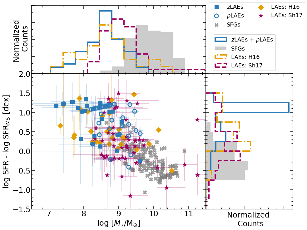
Figure 6 shows the distribution of properties of LAEs and SFGs, derived from SED fitting. The median values for the individual parameters for both the samples are shown as dashed vertical lines. In Table 1, we show the quartile values of these parameters for LAEs, LAEs, all LAEs together, and SFGs.
We find that the sample of LAEs (both LAEs and LAEs) contain young populations. The minimum age of the sample is restricted to be 10 Myr via SED fitting. However, it is possible that the galaxies with this borderline age from SED fitting might have ages less than 10 Myr. These are most probably compact galaxies with short dynamical timescales (see Section IV.3). All LAEs are found to be younger than 1 Gyr, with a median of 20 Myr. Given the typical uncertainties ( 40 Myr) in this parameter, any interpretations regarding the age should be carefully considered. The LAEs also have low dust reddening values, 0 E(BV) 0.26 mag, with a median of 0.08 mag. The LAEs are on average older and have more dust content than the LAEs (Table 1).
The sample of LAEs have stellar masses ranging from 7.2 9.6, with a median of 8.6. The SFRs measured for the LAEs range from 0.8 to 100 , with a median of 10 . These are in agreement with the measurements of stellar masses and SFRs in typical LAEs detected using narrow-band techniques at z 2 3 (Nilsson et al. 2011; Vargas et al. 2014; Sandberg et al. 2015; Shimakawa et al. 2017; Hao et al. 2018; Kusakabe et al. 2018). We also find that the LAEs are on average more massive and have higher SFRs compared to LAEs.
Table 1 shows the KS test results between the LAEs and LAEs for the different parameters. Even though both the samples are selected using the same criterion, the p-values for stellar mass and SFR, in particular, suggest that the two distributions may not share the same parent sample. LAEs with fainter (or less luminous) Ly emission tend to be redder and more massive, similar to what we have observed (Pentericci et al. 2009; Finkelstein et al. 2011; Hathi et al. 2016; Du et al. 2018; Du et al. 2021; Reddy et al. 2022, e.g., ). Additionally, the LAEs might have a possible low-redshift contamination, and the lack of spectroscopic redshifts introduces higher uncertainties in the SED fitting results.
On comparing the LAEs with the SFGs, we find that the LAEs are younger and have slightly lower dust content than SFGs. In fact, the median age of the SFGs is 1 Gyr, which is closer to the upper limit of the age of the LAEs. Additionally, the LAEs are on average less massive and have similar SFRs compared to SFGs. The KS test for all the parameters clearly suggests that the two samples have different underlying distributions (Table 1). We explore the location of LAEs and SFGs on the star-forming main sequence diagram below.
IV.2.2 Star-Forming Main Sequence
The position of typical star-forming galaxies in - SFR space follows a power law, often called the star-forming main sequence (Brinchmann et al. 2004; Daddi et al. 2007; Elbaz et al. 2007; Noeske et al. 2007, SFMS;). Some studies have found LAEs to lie above the SFMS (Hagen et al. 2014; Vargas et al. 2014; Hagen et al. 2016; Hao et al. 2018), while others found LAEs on the SFMS (Shimakawa et al. 2017; Kusakabe et al. 2018). The SFMS evolves with redshift, and these comparisons should be made with galaxies at similar redshifts. The location of a galaxy on the SFMS can help us understand the “mode” of star formation happening within it. Galaxies that lie on the SFMS are considered to be “normal” star-forming galaxies, while galaxies undergoing a current burst of star formation tend to reside above this sequence. Understanding the location of LAEs relative to the main sequence can provide clues to the star formation history of the LAEs.
Figure 7 shows the versus plot for the LAEs and SFGs. Two other LAE samples from Hagen et al. 2016 at z 2 (referred to as H16) and Shimakawa et al. 2017 at z 2.5 (referred to as Sh17) are also plotted. The stellar masses and SFRs from Shimakawa et al. 2017 were computed from the SED fitting technique assuming a Chabrier IMF (Chabrier 2003). We multiply them by 1.897, in order to scale them to Salpeter IMF, for consistency with the other data shown in Figure 7. Parametrizations for the SFMS computed by Whitaker et al. 2014, Schreiber et al. 2015, and Shivaei et al. 2015 are overplotted and extended to lower masses () in dotted, dashed, and solid lines respectively. The artificial tight relation between the stellar mass and SFR, as demonstrated by blue points in the figure, is due to the young ages of the LAEs. Both SFR and depend on the normalization of the best-fit SED to the photometry. As a result, these two parameters are tightly correlated, especially for a constant star formation history model.
We find that most of the LAEs lie above the SFMS relation, indicating an elevated SFR for their stellar mass. This suggests that most LAEs may be undergoing a bursty mode of star formation. In order to explore how much the LAEs deviate from the SFMS, we plot the separation of galaxies from the SFMS (), parametrized by Shivaei et al. 2015, as a function of stellar mass in Figure 8. The horizontal dashed line denotes the expected values when a galaxy lies on the SFMS for a given . We are assuming that the SFMS parametrization extends to lower masses as well. Seventeen out of 62 ( 28 %) LAEs lie within 2 of the SFMS, but the majority of sources ( 70%) are well above the relation. Their star forming modes range from “bursty” to “normal” star formation. For a given stellar mass, LAEs typically have a more star-bursty nature compared to SFGs. However, the position of galaxies on the SFMS will also depend on their ages. The larger separations from SFMS indicates that for a given stellar mass, LAEs tend to be younger than SFGs. More massive LAEs lie on the main sequence compared to their less massive counterparts (Santos et al. 2020, similar to ). However, it is possible that we are missing galaxies that have low masses as well as low SFRs. Continuum-based searches are magnitude-limited and tend to select higher-mass galaxies, while Ly emission based searches select galaxies with higher Ly emission, which is mostly a result of higher SFRs.

The top and right panels of Figure 8 show normalized histograms of stellar masses and of the different galaxy populations, respectively. The observed peak in is from the LAEs that border the artificial relation in Figure 7. Combining our results with those of LAEs in the literature, we observe that LAEs, on average, lie above the SFMS compared to typical SFGs. On the other hand, LAEs are, on average 1.5 dex less massive than the SFGs. This indicates that galaxies selected via Ly emission line almost always probe the low-mass end of the galaxy mass function and have higher specific SFRs (sSFRs), on average, compared to typical SFGs.
IV.3 Morphology of LAEs
Previous studies have shown that LAEs are compact in the rest-frame UV and optical continuum (Bond et al. 2009; Gronwall et al. 2011; Bond et al. 2012; Malhotra et al. 2012; Paulino-Afonso et al. 2018; Shibuya et al. 2019). We compute the sizes of our sample of LAEs using the HST images with the aim of estimating their SFR surface densities as well as for comparing them to typical SFGs. The sizes and SFR surface densities of MOSDEF SFGs are presented in Reddy et al. 2022, and we will refer to that study for comparison.
IV.3.1 Rest-frame Optical Size Measurements
To measure the sizes from HST images, we first compute the PSF of these images using GALFIT (Peng et al. 2010). We find stars by running Source Extractor on all the images based on the CLASS_STAR parameter. We then run GALFIT on these stars with a Sérsic2D profile (Sérsic 1963) by fixing the Sérsic index, = 0.5, which is identical to a 2D-Gaussian profile. The resulting effective radius () is taken as the effective radius of the PSF. GALFIT fails to converge when trying to run with an input PSF, suggesting that the LAEs are barely resolved. To circumvent this, we estimate the LAE sizes by running GALFIT without an input PSF profile to the fitting tool. This results in sizes from the images that are not yet corrected for the PSF. We fix = 1 to compute the effective radius of galaxies using a Sérsic2D profile. Given the limiting PSF resolution, there is no obvious difference in the results when we vary the value of the Sérsic index. We correct the resulting radius for PSF by subtracting of the PSF from it in quadrature. In order to check the validity of our sizes, we compute of all the LAEs using the continuum images using the same method as above. The sizes derived from and images are consistent within the uncertainties.
We consider all the sources that have within 2 of the PSF as unresolved sources, and we set of the PSF as the upper limit to their sizes. The left panel of Figure 9 shows the distribution of these sizes. We find that 37 out of 64 LAE candidates () are unresolved ( 1 kpc). If we consider the fraction of unresolved galaxies as a degree of compactness for a particular population of galaxies, then most studies of LAEs find a higher fraction of unresolved galaxies than LBGs or typical SFGs at a given stellar mass. SFGs with stellar masses at z 23, are more spatially extended, with sizes in the range of (Law et al. 2012; Shibuya et al. 2015). Additionally, studies have found that LAEs are smaller than typical SFGs across all redshifts (Paulino-Afonso et al. 2018).
LAEs have sizes that are independent of redshift (Malhotra et al. 2012; Kim et al. 2021). This is in contrast with the size evolution observed in SFGs and LBGs (Shibuya et al. 2015). This means that galaxies selected based on their strong Ly emission are mostly compact in nature, suggesting that Ly escape might be related to the sizes of galaxies (Section V.2).
IV.3.2 Star-Formation-Rate Surface Densities
The distribution of star formation in galaxies may influence the escape of Ly photons from them (Section I). To probe this connection, we measure the star-formation-rate surface density, :
| (13) |
In the middle panel of Figure 9, we show the distribution of of our sample of LAEs. We find lower limits for the unresolved sources, which are shown as a dotted histogram in the figure. From resolved sources, we find that the LAEs have . This is higher than the values for typical SFGs at , that have (Shibuya et al. 2015; Reddy et al. 2022).
Previous studies suggest that the gravitational potential may also play a role in Ly escape (Kim et al. 2021; Reddy et al. 2022). We consider stellar mass as a proxy for this potential (e.g., see Reddy et al. 2022, for more details) and compute specific star-formation-rate surface density, , to quantify this effect.
| (14) |
The distribution of is shown in the right panel of Figure 9, which includes lower limits for unresolved sources. The LAEs have , while SFGs typically have (Reddy et al. 2022).
IV.4 Proxies for Escape


We quantify the escape of Ly photons using three different measurements: the Ly equivalent width (); the ratio of Ly to [O ii] luminosity (Ly/[O ii]); and the escape fraction (). It is important to note that we are measuring the Ly escape only along the line-of-sight, and are not accounting for photons that are resonantly scattered into the diffuse halo. Even though these proxies are sensitive to the gas covering fraction and the dust content in galaxies, they are different measures of the observed Ly emission.
The equivalent width of the Ly emission () is the least model-dependent proxy for the Ly escape (Sobral & Matthee 2019). The calculation of for LAEs and SFGs is described in Section IV.1. In the left panel of Figure 10, we show the distribution of for LAEs and SFGs. The LAEs have higher ranging from 20250 Å with a median of Å. In contrast, the SFGs with observable Ly emission have a median of Å. This difference is mostly by selection, since galaxies with high are likely to be selected via narrow-band imaging and are more likely to be spectroscopically confirmed.
The ratio of Ly to [O ii] luminosity is another possible proxy for the escape of Ly, which depends on the distribution of gas and dust in the galaxy. Unlike Ly emission, [O ii] photons are not resonant in nature, and therefore Ly/[O ii] can be used as an independent measure of Ly escape. The Ly and [O ii] flux measurements are presented in Section IV.1. The middle panel of Figure 10 shows the distribution of Ly/[O ii] ratio of LAEs and SFGs. In cases where there is no significant [O ii] emission, we have lower limits on the Ly/[O ii] ratio, as shown by the dotted histograms in the plot. We find that (Ly/[O ii]) ranges from 0.142.06, with a median 0.91. The distribution also shows that LAEs have higher Ly/[O ii], on average, compared to SFGs, due to the higher Ly escape in LAEs. However, [O ii] emission depends on the ionization parameter and metallicity of galaxies, as discussed below.
Figure 11 shows how the intrinsic Ly/[O ii] is predicted to vary with nebular metallicity, , based on photoionization modeling. To compute this relationship, we use the photoionization modeling code CLOUDY (Ferland et al. 2013) with an intrinsic ionizing spectrum set by the BPASS (Eldridge et al. 2017) constant star formation models, with a stellar metallicity of 0.2 and an age of . We then use these models to compute the expected Ly/[O ii] ratio as a function of , where the ionization parameter, , is fixed to the value predicted by the anti-correlation between and found in local H ii regions (Pérez-Montero 2014). As observed in the middle panel of Figure 10, eight LAEs (13%) have (Ly/[O ii]) 1.5, on the high end of what is expected. Because these Ly/[O ii] do not account for the potentially large fraction of Ly photons that are resonantly scattered out of the photometric aperture, these ratios are effectively lower limits. This suggests that these galaxies are extremes in the parameter space shown in Figure 11. To produce such high Ly/[O ii] ratios, they should either have very low nebular metallicities, , and/or very high ionization parameters, , similar to the values measured for other LAE samples at high redshift (Finkelstein et al. 2011; Nakajima et al. 2012; Nakajima et al. 2013).
Finally, Ly escape fraction (), which is defined as the ratio of observed Ly luminosity to the intrinsic Ly luminosity produced in a galaxy, is the most commonly used parameter to study the escape of Ly in galaxies. The estimate of escape fraction depends on several assumptions such as metallicities, star formation histories, and dust attenuation curves. We calculate the intrinsic Ly luminosity using the SFR computed from the SED fitting and the CLOUDY models (Ferland et al. 2013). The ionizing photon luminosity per unit SFR for this model is 9.259 . Assuming Case-B recombination, the intrinsic H luminosity is, (Leitherer & Heckman 1995), and the SFR [] (Reddy et al. 2022). We use this relation to compute the intrinsic H luminosity from the SED-based SFR. This assumes that the ionizing photons neither escape nor get absorbed by dust prior to photoionizing hydrogen. Assuming a stellar metallicity of 0.2 , an age of , a nebular metallicity of , and an ionization parameter, of -2.0, yields Ly/H from these models. We use this ratio to compute the intrinsic Ly luminosity from H luminosity, which, along with the observed Ly luminosities (Section IV.1), is used to calculate for the LAEs and SFGs.

| Proxy for Ly escape | ||||
|---|---|---|---|---|
| Only LAEs | LAEs+MOSDEF | Only LAEs | LAEs+MOSDEF | |
| -0.47 (0.0001) | -0.72 (1.4 ) | -0.50 (2.9 ) | -0.02 (0.80) | |
| Ly/[O ii] | -0.24 (0.06) | -0.73 (7.4 ) | -0.39 (0.002) | -0.05 (0.59) |

Three of the LAEs in our sample have computed escape fractions greater than 1. Two of these sources (DENS1_86 and DENS1_356) have extremely faint continua, resulting in poor SED fits. The third source (FIELD4_124) has high Ly luminosity () and is possibly an active galaxy (AGN) (Sobral et al. 2018; Zhang et al. 2021).
The right panel of Figure 10 shows the distribution of escape fraction of LAEs in comparison with the SFGs. Given the observed , these distributions are typical for galaxies at similar and lower redshifts (Matthee et al. 2016; Yang et al. 2017; Weiss et al. 2021; Reddy et al. 2022). The median escape fraction of the SFGs ( 4.8%) is similar to the escape fraction expected at z 23 (Hayes et al. 2010; Sobral et al. 2017). The LAEs however have a median escape fraction of 13.5%, which is significantly higher and is closer to the escape fraction observed at z 6 (see Figures 1 and 4 in Hayes et al. 2011). It has been observed that Ly escape is correlated with the escape of ionizing photons (Marchi et al. 2017; Marchi et al. 2018; Steidel et al. 2018; Pahl et al. 2021), and galaxies with high ionizing escape fractions are often bright LAEs at similar redshifts (Naidu et al. 2022). The comparable escape fractions of the LAEs to the escape fraction observed at z 6 suggests that these are probably low-redshift analogs of galaxies that contributed to reionization.
V Ly escape and galaxy properties
V.1 Dependence on Stellar Mass and SFR
To understand the physical driver of high Ly escape in LAEs compared to typical SFGs, we search for any significant trends with galaxy properties. Figure 12 shows how and the measured Ly/[O ii] luminosity ratio depend on the stellar masses and SFRs of LAEs and SFGs. In each panel, the filled blue squares and open blue circles represent LAEs and LAEs, respectively, and gray crosses denote SFGs. Furthermore, the red square, red circle, and the black cross and their corresponding error bars mark the median and interquartile ranges of the individual samples. We study the strength of correlations using the Spearman correlation test (Table 2). Note that we are not considering in this analysis, as the calculation of is dependent on the SFRs derived from the SED fitting. As mentioned in the previous section, we consider and Ly/[O ii] as proxies for Ly escape.
The top panels show and Ly/[O ii] as a function of stellar mass. As expected, LAEs have higher and Ly/[O ii] ratios. From Table 2, we see that there is a possible anti-correlation between vs , as well as between Ly/[O ii] vs , when we consider both the LAE sample and MOSDEF SFGs together. When we consider the LAE sample alone, there is a moderate anti-correlation between Ly escape proxies and stellar mass. Focusing on the median points in these panels, we see that Ly escape has a clear dependence on the stellar mass of star-forming galaxies. This is similar to what has been observed in many previous studies (Matthee et al. 2016; Oyarzún et al. 2016; Oyarzún et al. 2017; Santos et al. 2020; Weiss et al. 2021). However, the sample may be incomplete in the lower-left regions of these two panels due to the sensitivity limits of both narrowband and continuum-based surveys.
The bottom panels of Figure 12 show the dependence of and Ly/[O ii] on the SFR of galaxies. When all LAEs and SFGs are considered, the Spearman coefficient for vs SFR is -0.02, while the coefficient for Ly/[O ii] vs SFR is -0.05. This suggests that there is no obvious correlation between Ly escape and SFR for these galaxies. This non-dependence of Ly escape on SFR is in contrast with several previous studies on LAEs and SFGs (Matthee et al. 2016; Oyarzún et al. 2017; Weiss et al. 2021). This is not surprising because the detection of correlation depends on the dynamic range in Ly escape and SFR probed by the different samples. As the SFR increases, the intrinsic Ly emission will increase along with the gas and dust column densities. This increase in gas and dust densities, in turn, will influence the emergent Ly emission. The observed non-dependence of Ly escape on SFR, along with the diverse range of SFRs in LAEs (Section IV.2.1) suggest that star formation alone is not the primary driver for the escape of Ly photons. The following subsections discuss the dependence of Ly escape on sizes and star-formation-rate surface densities.
V.2 Dependence on the Sizes
Figure 13 shows the dependence of , Ly/[O ii] luminosity ratio, and on the compactness of galaxies. All the points plotted near 1 kpc are unresolved galaxies that have sizes 1 kpc. The Ly escape in LAEs spans a broad range of values, and is higher for unresolved galaxies on average, compared to resolved galaxies. The left and right stars in each of the panels show the median values of the Ly escape proxies for unresolved and resolved sources, respectively. The error bars denote the interquartile range of the different distributions. These median values suggest a possible 2 anti-correlation between and size of the galaxy.
From Figure 13, we also find that the fraction of resolved LAEs ( 63%) is higher than the fraction of resolved LAEs ( 18%). The LAEs are spectroscopically confirmed due to the stronger Ly emission from them, compared to LAEs. This also suggests a dependence of on galaxy sizes.
Bond et al. 2012 studied the rest-frame UV sizes of z 2.1 and z 3.1 LAEs and found a systematic trend that higher LAEs have smaller median sizes compared to the lower samples. This dependence of Ly escape on galaxy sizes is also seen in typical SFGs. Law et al. 2012 studied 200 star-forming galaxies and uncovered a higher fraction of Ly emission in galaxies with compact morphologies. More recently, Weiss et al. 2021 found that is anti-correlated with for [OIII]-emitting galaxies (Reddy et al. 2022, also see). Kim et al. 2021 studied nearby Green Pea galaxies which emit Ly emission and found that is dependent on their sizes. Paulino-Afonso et al. 2018 also found an anti-correlation between and the UV sizes of high-redshift LAEs from 2 6. These studies suggest that this dependence is independent of redshift. Therefore, galaxy sizes clearly play an important role in the escape of Ly photons.
V.3 Dependence on Star-Formation-Rate Surface Densities

Observational studies suggest a possible correlation between Ly escape fraction and (Heckman et al. 2011; Verhamme et al. 2017; Marchi et al. 2019; Reddy et al. 2022). Furthermore, the gravitational potential of the galaxy, encoded in specific star-formation-rate surface density, can also influence the escape of Ly photons. In Figure 14, we compare our sample of LAEs with those obtained for MOSDEF SFGs from Reddy et al. 2022 (similar to their Figure 21). The LAEs and LAEs are shown as closed squares and open circles, respectively. We further divide the LAEs into low-mass ( 8.5) and high-mass ( 8.5) sources, shown by blue and red markers, respectively. The SFGs have a median stellar mass, 10.
In Figure 14, the LAEs that have only lower limits to their and are the sources that are unresolved, with sizes 1 kpc. From the left panel, we see that the sources that are resolved have similar , but higher , compared to SFGs. This suggests that there is an additional factor beyond that modulate . For galaxies with a fixed , we see that the sources with lower masses have higher . This can be also seen from the right panel of the figure, where LAEs have higher , on average, compared to SFGs. This highlights the effect of stellar mass (and therefore the gravitational potential) on the Ly escape (Section V.1 and Figure 12).
These results reinforce the argument that the distribution of star formation is a key ingredient for Ly escape. The feedback associated with compact star formation will lead to outflows, that will in turn create low-density channels in the ISM. These low-density columns provide pathways for the Ly photons to propagate and escape. The gravitational potential (or stellar mass) also plays a crucial role in this scenario. The shallow potential well of low-mass sources makes it harder for them to retain the gas that is pushed out via winds and outflows. As we are measuring the Ly photons along the line-of-sight, this physical interpretation is highly dependent on the orientation of galaxies. Large-scale deep observations of galaxies across the multi-wavelength regime will give further clues about the dependence of Ly escape on gravitational potential and sizes of galaxies.
V.4 Dependence on the Environment

| LAEs Group | SFR | (Ly/[O ii]) | |||
|---|---|---|---|---|---|
| LAEs | 0.35 | 0.45 | 0.27 | 0.98 | 0.61 |
| All LAEs | 0.18 | 0.39 | 0.17 | 0.51 | 0.89 |
In this subsection, we investigate whether Ly escape has any dependence on the environment of LAEs. In Section II.1, we mentioned that we have HST imaging of LAEs in seven fields, three of which are in dense regions, as measured by Prescott et al. 2008. Thus, we divide our LAEs into high-density (DENS) and low-density (FIELD) sources, based on their proximity to the Ly blob. Some LAE candidates have either a close companion or exhibit an extended component visible in the HST images. These companions and/or components are typically not resolved in the ground-based images, and may indicate a close physical companion. Out of the 62 LAEs in our sample, we identify 14 sources which exhibit such components within 1.5″. We consider the Ly escape of this subset in comparison with the rest of the LAEs.
Figure 15 shows the distribution of different Ly escape proxies for LAEs in low and high density environments. The dark and light green histograms are LAEs in the DENS and FIELD regions, respectively. We perform KS tests for the different proxies between all LAEs in these two groups. We also repeat the tests by considering just the LAEs, since the spectroscopic redshifts yield more accurate environmental information (Table 3). From the p-values, we cannot reject the null hypothesis that the Ly escape for DENS and FIELD regions are similar. Additionally, the black histogram with circles in the figure are the LAEs with close neighbors and/or extended components. The p-values from the KS tests between these 14 LAEs and the rest of the LAEs for , Ly/[O ii] ratio, and are 0.26, 0.35, and 0.42, respectively. This suggests that given our rough definition of environment, Ly escape does not depend on the local environment of the LAEs in this sample.
Table 3 also shows the p-values from the KS tests for stellar masses and SFRs between LAEs in DENS and FIELD regions. For both LAEs and all LAEs together, we find that the stellar masses and SFRs are statistically similar for LAEs in these different environments. We cannot make any comparisons between the sizes of these galaxies because of the high fraction of unresolved sources and small numbers of resolved LAEs in the individual groups. However, given that most of the LAEs in our sample are compact, the of the LAEs in DENS and FIELD environments are likely similar. This argument supports our earlier result that the star formation in a low-mass, compact galaxy is key to the Ly escape in galaxies, irrespective of the local environment.
VI Conclusions
In an effort to understand the mechanisms that lead to Ly escape in LAEs, we study 62 LAEs from seven HST fields using multi-wavelength photometry. Out of these, 27 sources have confirmed spectroscopic redshifts between 2.55 z 2.75. In addition to broad-band photometry in , , , , and filters, we also have medium-band photometry in and bands that probe the Ly and [O ii] emission lines, respectively in this redshift range. We considered a comparison sample of 136 typical SFGs that are part of the MOSDEF/LRIS sample (Section II.2).
We obtained the stellar masses, SFRs, ages, and dust content of all the LAEs using the SED fitting technique (Section IV.2). We also computed LAE sizes by running GALFIT on the HST images (Section IV.3). Finally, we considered three proxies for the Ly escape: the Ly equivalent width (); the Ly/[O ii] luminosity ratio; and the Ly escape fraction () (Section IV.4). Using these proxies and studying their correlations with the LAE properties, we conclude:
- •
LAEs typically probe low-mass (7.2 9.6), young (age 1 Gyr), star-forming galaxies (0.8 ) with low dust content (E(BV) 0.26 mag). LAEs are more massive, star-forming, older, and redder compared to LAEs. Furthermore, LAEs and SFGs have different underlying distributions. LAEs have lower ages, lower masses, similar SFRs, and less dust content compared to SFGs at similar redshifts (Section IV.2.1).
- •
LAEs have a wide range of SFRs, and have higher sSFRs compared to SFGs. On average, less massive LAEs lie above the SFMS, compared to their massive counterparts (Section IV.2.2)
- •
Almost 60% of the LAEs are unresolved, even with HST resolution, indicating that these galaxies are compact ( 1 kpc). LAEs also have comparable and higher compared to SFGs (Section IV.3).
- •
LAEs have higher , higher Ly/[O ii] luminosity ratios, and higher compared to SFGs. By comparing the Ly/[O ii] ratios with expected model values, we found that some LAEs are extreme galaxies with low nebular metallicities () and/or high ionization parameters ( ). Additionally, the of LAEs is similar to the escape fraction observed at z 6, suggesting that these LAEs may be low-redshift analogs of galaxies that contributed to reionization (Section IV.4).
- •
The escape of Ly in galaxies is anti-correlated with stellar mass, but shows no obvious dependence on SFR (Section V.1).
- •
The Ly escape has a wide range of values for unresolved LAEs, and is on average higher for unresolved LAEs compared to their resolved counterparts (Section V.2).
- •
For a given , the lower-mass LAEs have higher than their more massive counterparts. This is consistent with a scenario where compact star formation in a low gravitational potential facilitates the escape of Ly, by creating low-column-density channels in the ISM via feedback. (Section V.3).
- •
Based on the local density of the HST fields, we do not observe any obvious dependence of nearby environment on the Ly escape from galaxies (Section V.4).
Upcoming surveys such as the One-hundred square-degree DECam Imaging in Narrowbands (ODIN) survey, the Legacy Survey of Space and Time with the Vera Rubin Telescope (Ivezić et al. 2019), and upcoming deep JWST NIRSPEC observations (Giardino et al. 2016), will provide us with large scale observations of LAEs in different environments across different epochs. These new datasets will help us understand the physics of Ly escape in more detail.
References
- Acquaviva et al. (2012) Acquaviva, V., Vargas, C., Gawiser, E., & Guaita, L. 2012, ApJ, 751, L26
- Adams et al. (2011) Adams, J. J., Blanc, G. A., Hill, G. J., et al. 2011, ApJS, 192, 5
- Arrabal Haro et al. (2018) Arrabal Haro, P., Rodríguez Espinosa, J. M., Muñoz-Tuñón, C., et al. 2018, arXiv e-prints, arXiv:1805.00477
- Arrabal Haro et al. (2020) —. 2020, MNRAS, 495, 1807
- Avila et al. (2012) Avila, R. J., Hack, W. J., & STScI AstroDrizzle Team. 2012, in American Astronomical Society Meeting Abstracts, Vol. 220, American Astronomical Society Meeting Abstracts #220, 135.13
- Bacon et al. (2017) Bacon, R., Conseil, S., Mary, D., et al. 2017, A&A, 608, A1
- Bertin & Arnouts (1996) Bertin, E., & Arnouts, S. 1996, A&AS, 117, 393
- Blanc et al. (2011) Blanc, G. A., Adams, J. J., Gebhardt, K., et al. 2011, ApJ, 736, 31
- Bond et al. (2009) Bond, N. A., Gawiser, E., Gronwall, C., et al. 2009, ApJ, 705, 639
- Bond et al. (2012) Bond, N. A., Gawiser, E., Guaita, L., et al. 2012, ApJ, 753, 95
- Borthakur et al. (2014) Borthakur, S., Heckman, T. M., Leitherer, C., & Overzier, R. A. 2014, Science, 346, 216
- Bradley et al. (2019) Bradley, L., Sipőcz, B., Robitaille, T., et al. 2019, astropy/photutils: v0.6, , , doi:10.5281/zenodo.2533376
- Brinchmann et al. (2004) Brinchmann, J., Charlot, S., White, S. D. M., et al. 2004, MNRAS, 351, 1151
- Bruzual & Charlot (2003) Bruzual, G., & Charlot, S. 2003, MNRAS, 344, 1000
- Carnall et al. (2018) Carnall, A. C., McLure, R. J., Dunlop, J. S., & Davé, R. 2018, MNRAS, 480, 4379
- Cen (2020) Cen, R. 2020, ApJ, 889, L22
- Chabrier (2003) Chabrier, G. 2003, PASP, 115, 763
- Cullen et al. (2020) Cullen, F., McLure, R. J., Dunlop, J. S., et al. 2020, MNRAS, 495, 1501
- Daddi et al. (2007) Daddi, E., Dickinson, M., Morrison, G., et al. 2007, ApJ, 670, 156
- De Barros et al. (2017) De Barros, S., Pentericci, L., Vanzella, E., et al. 2017, A&A, 608, A123
- Dey et al. (2016) Dey, A., Lee, K.-S., Reddy, N., et al. 2016, ApJ, 823, 11
- Dey et al. (2005) Dey, A., Bian, C., Soifer, B. T., et al. 2005, ApJ, 629, 654
- Dijkstra (2017) Dijkstra, M. 2017, arXiv e-prints, arXiv:1704.03416
- Dressel (2012) Dressel, L. 2012, Wide Field Camera 3 Instrument Handbook for Cycle 21 v. 5.0
- Du et al. (2018) Du, X., Shapley, A. E., Reddy, N. A., et al. 2018, ApJ, 860, 75
- Du et al. (2021) Du, X., Shapley, A. E., Topping, M. W., et al. 2021, arXiv e-prints, arXiv:2103.15824
- Elbaz et al. (2007) Elbaz, D., Daddi, E., Le Borgne, D., et al. 2007, A&A, 468, 33
- Eldridge et al. (2017) Eldridge, J. J., Stanway, E. R., Xiao, L., et al. 2017, PASA, 34, e058
- Fabricant et al. (2005) Fabricant, D., Fata, R., Roll, J., et al. 2005, PASP, 117, 1411
- Ferland et al. (2013) Ferland, G. J., Porter, R. L., van Hoof, P. A. M., et al. 2013, Rev. Mexicana Astron. Astrofis., 49, 137
- Finkelstein et al. (2011) Finkelstein, S. L., Cohen, S. H., Moustakas, J., et al. 2011, ApJ, 733, 117
- Finkelstein et al. (2009) Finkelstein, S. L., Rhoads, J. E., Malhotra, S., & Grogin, N. 2009, ApJ, 691, 465
- Finkelstein et al. (2007) Finkelstein, S. L., Rhoads, J. E., Malhotra, S., Pirzkal, N., & Wang, J. 2007, ApJ, 660, 1023
- Gawiser et al. (2006) Gawiser, E., van Dokkum, P. G., Gronwall, C., et al. 2006, ApJ, 642, L13
- Gawiser et al. (2007) Gawiser, E., Francke, H., Lai, K., et al. 2007, ApJ, 671, 278
- Giardino et al. (2016) Giardino, G., de Oliveira, C. A., Arribas, S., et al. 2016, in Astronomical Society of the Pacific Conference Series, Vol. 507, Multi-Object Spectroscopy in the Next Decade: Big Questions, Large Surveys, and Wide Fields, ed. I. Skillen, M. Balcells, & S. Trager, 305
- Giavalisco (2002) Giavalisco, M. 2002, ARA&A, 40, 579
- Gnedin et al. (2008) Gnedin, N. Y., Kravtsov, A. V., & Chen, H.-W. 2008, ApJ, 672, 765
- Gordon et al. (2003) Gordon, K. D., Clayton, G. C., Misselt, K. A., Landolt, A. U., & Wolff, M. J. 2003, ApJ, 594, 279
- Grogin et al. (2011) Grogin, N. A., Kocevski, D. D., Faber, S. M., et al. 2011, ApJS, 197, 35
- Gronwall et al. (2011) Gronwall, C., Bond, N. A., Ciardullo, R., et al. 2011, ApJ, 743, 9
- Guaita et al. (2011) Guaita, L., Acquaviva, V., Padilla, N., et al. 2011, ApJ, 733, 114
- Hagen et al. (2014) Hagen, A., Ciardullo, R., Gronwall, C., et al. 2014, ApJ, 786, 59
- Hagen et al. (2016) Hagen, A., Zeimann, G. R., Behrens, C., et al. 2016, ApJ, 817, 79
- Hao et al. (2018) Hao, C.-N., Huang, J.-S., Xia, X., et al. 2018, ApJ, 864, 145
- Hathi et al. (2016) Hathi, N. P., Le Fèvre, O., Ilbert, O., et al. 2016, A&A, 588, A26
- Hayes et al. (2011) Hayes, M., Schaerer, D., Östlin, G., et al. 2011, ApJ, 730, 8
- Hayes et al. (2010) Hayes, M., Östlin, G., Schaerer, D., et al. 2010, Nature, 464, 562
- Heckman et al. (2011) Heckman, T. M., Borthakur, S., Overzier, R., et al. 2011, ApJ, 730, 5
- Herenz et al. (2020) Herenz, E. C., Hayes, M., & Scarlata, C. 2020, A&A, 642, A55
- Herrero Alonso et al. (2021) Herrero Alonso, Y., Krumpe, M., Wisotzki, L., et al. 2021, A&A, 653, A136
- Hinshaw et al. (2013) Hinshaw, G., Larson, D., Komatsu, E., et al. 2013, ApJS, 208, 19
- Hoag et al. (2019) Hoag, A., Treu, T., Pentericci, L., et al. 2019, MNRAS, 488, 706
- Hong et al. (2014) Hong, S., Dey, A., & Prescott, M. K. M. 2014, PASP, 126, 1048
- Huang et al. (2021) Huang, Y., Lee, K.-S., Shi, K., et al. 2021, arXiv e-prints, arXiv:2104.11354
- Ivezić et al. (2019) Ivezić, Ž., Kahn, S. M., Tyson, J. A., et al. 2019, ApJ, 873, 111
- Izotov et al. (2016) Izotov, Y. I., Orlitová, I., Schaerer, D., et al. 2016, Nature, 529, 178
- Jannuzi & Dey (1999) Jannuzi, B. T., & Dey, A. 1999, in Astronomical Society of the Pacific Conference Series, Vol. 191, Photometric Redshifts and the Detection of High Redshift Galaxies, ed. R. Weymann, L. Storrie-Lombardi, M. Sawicki, & R. Brunner, 111
- Jaskot et al. (2019) Jaskot, A. E., Dowd, T., Oey, M. S., Scarlata, C., & McKinney, J. 2019, ApJ, 885, 96
- Jiang et al. (2013) Jiang, L., Egami, E., Fan, X., et al. 2013, ApJ, 773, 153
- Kakiichi & Gronke (2021) Kakiichi, K., & Gronke, M. 2021, ApJ, 908, 30
- Kashino et al. (2022) Kashino, D., Lilly, S. J., Renzini, A., et al. 2022, ApJ, 925, 82
- Khostovan et al. (2019) Khostovan, A. A., Sobral, D., Mobasher, B., et al. 2019, MNRAS, 489, 555
- Kim et al. (2020) Kim, K., Malhotra, S., Rhoads, J. E., Butler, N. R., & Yang, H. 2020, ApJ, 893, 134
- Kim et al. (2021) Kim, K. J., Malhotra, S., Rhoads, J. E., & Yang, H. 2021, ApJ, 914, 2
- Kimm et al. (2019) Kimm, T., Blaizot, J., Garel, T., et al. 2019, MNRAS, 486, 2215
- Knapen & Cisternas (2015) Knapen, J. H., & Cisternas, M. 2015, ApJ, 807, L16
- Koekemoer et al. (2011) Koekemoer, A. M., Faber, S. M., Ferguson, H. C., et al. 2011, ApJS, 197, 36
- Kornei et al. (2010) Kornei, K. A., Shapley, A. E., Erb, D. K., et al. 2010, ApJ, 711, 693
- Kriek et al. (2015) Kriek, M., Shapley, A. E., Reddy, N. A., et al. 2015, ApJS, 218, 15
- Kusakabe et al. (2018) Kusakabe, H., Shimasaku, K., Ouchi, M., et al. 2018, PASJ, 70, 4
- Lai et al. (2008) Lai, K., Huang, J.-S., Fazio, G., et al. 2008, ApJ, 674, 70
- Law et al. (2012) Law, D. R., Steidel, C. C., Shapley, A. E., et al. 2012, ApJ, 745, 85
- Leclercq et al. (2020) Leclercq, F., Bacon, R., Verhamme, A., et al. 2020, A&A, 635, A82
- Leitherer & Heckman (1995) Leitherer, C., & Heckman, T. M. 1995, ApJS, 96, 9
- Lemaux et al. (2018) Lemaux, B. C., Le Fèvre, O., Cucciati, O., et al. 2018, A&A, 615, A77
- Lemaux et al. (2021) Lemaux, B. C., Fuller, S., Bradač, M., et al. 2021, MNRAS, 504, 3662
- Luo et al. (2014) Luo, W., Yang, X., & Zhang, Y. 2014, ApJ, 789, L16
- Ma et al. (2016) Ma, X., Hopkins, P. F., Kasen, D., et al. 2016, MNRAS, 459, 3614
- Ma et al. (2020) Ma, X., Quataert, E., Wetzel, A., et al. 2020, MNRAS, 498, 2001
- Malavasi et al. (2021) Malavasi, N., Lee, K.-S., Dey, A., et al. 2021, arXiv e-prints, arXiv:2103.12750
- Malhotra et al. (2012) Malhotra, S., Rhoads, J. E., Finkelstein, S. L., et al. 2012, ApJ, 750, L36
- Marchi et al. (2017) Marchi, F., Pentericci, L., Guaita, L., et al. 2017, A&A, 601, A73
- Marchi et al. (2018) —. 2018, A&A, 614, A11
- Marchi et al. (2019) —. 2019, A&A, 631, A19
- Matthee et al. (2016) Matthee, J., Sobral, D., Oteo, I., et al. 2016, MNRAS, 458, 449
- Matthee et al. (2021) Matthee, J., Sobral, D., Hayes, M., et al. 2021, MNRAS, 505, 1382
- McLean et al. (2012) McLean, I. S., Steidel, C. C., Epps, H. W., et al. 2012, in Society of Photo-Optical Instrumentation Engineers (SPIE) Conference Series, Vol. 8446, Ground-based and Airborne Instrumentation for Astronomy IV, ed. I. S. McLean, S. K. Ramsay, & H. Takami, 84460J
- McLinden et al. (2014) McLinden, E. M., Rhoads, J. E., Malhotra, S., et al. 2014, MNRAS, 439, 446
- Miyazaki et al. (2002) Miyazaki, S., Komiyama, Y., Sekiguchi, M., et al. 2002, PASJ, 54, 833
- Momose et al. (2014) Momose, R., Ouchi, M., Nakajima, K., et al. 2014, MNRAS, 442, 110
- Moreno et al. (2021) Moreno, J., Torrey, P., Ellison, S. L., et al. 2021, MNRAS, 503, 3113
- Naidu et al. (2020) Naidu, R. P., Tacchella, S., Mason, C. A., et al. 2020, ApJ, 892, 109
- Naidu et al. (2022) Naidu, R. P., Matthee, J., Oesch, P. A., et al. 2022, MNRAS, 510, 4582
- Nakajima et al. (2013) Nakajima, K., Ouchi, M., Shimasaku, K., et al. 2013, ApJ, 769, 3
- Nakajima et al. (2012) —. 2012, ApJ, 745, 12
- Nilsson et al. (2011) Nilsson, K. K., Östlin, G., Møller, P., et al. 2011, A&A, 529, A9
- Nilsson et al. (2007) Nilsson, K. K., Møller, P., Möller, O., et al. 2007, A&A, 471, 71
- Noeske et al. (2007) Noeske, K. G., Faber, S. M., Weiner, B. J., et al. 2007, ApJ, 660, L47
- Oke & Gunn (1983) Oke, J. B., & Gunn, J. E. 1983, ApJ, 266, 713
- Oke et al. (1995) Oke, J. B., Cohen, J. G., Carr, M., et al. 1995, PASP, 107, 375
- Ono et al. (2010) Ono, Y., Ouchi, M., Shimasaku, K., et al. 2010, MNRAS, 402, 1580
- Ouchi et al. (2020) Ouchi, M., Ono, Y., & Shibuya, T. 2020, ARA&A, 58, 617
- Ouchi et al. (2003) Ouchi, M., Shimasaku, K., Furusawa, H., et al. 2003, ApJ, 582, 60
- Oyarzún et al. (2017) Oyarzún, G. A., Blanc, G. A., González, V., Mateo, M., & Bailey, John I., I. 2017, ApJ, 843, 133
- Oyarzún et al. (2016) Oyarzún, G. A., Blanc, G. A., González, V., et al. 2016, ApJ, 821, L14
- Pahl et al. (2021) Pahl, A. J., Shapley, A., Steidel, C. C., Chen, Y., & Reddy, N. A. 2021, MNRAS, 505, 2447
- Partridge & Peebles (1967) Partridge, R. B., & Peebles, P. J. E. 1967, ApJ, 147, 868
- Paulino-Afonso et al. (2018) Paulino-Afonso, A., Sobral, D., Ribeiro, B., et al. 2018, MNRAS, 476, 5479
- Peng et al. (2010) Peng, C. Y., Ho, L. C., Impey, C. D., & Rix, H.-W. 2010, AJ, 139, 2097
- Pentericci et al. (2009) Pentericci, L., Grazian, A., Fontana, A., et al. 2009, A&A, 494, 553
- Pentericci et al. (2007) —. 2007, A&A, 471, 433
- Pérez-Montero (2014) Pérez-Montero, E. 2014, MNRAS, 441, 2663
- Pirzkal et al. (2007) Pirzkal, N., Malhotra, S., Rhoads, J. E., & Xu, C. 2007, ApJ, 667, 49
- Pirzkal et al. (2010) Pirzkal, N., Viana, A., & Rajan, A. 2010, The WFC3 IR ’Blobs”, Space Telescope WFC Instrument Science Report, ,
- Prescott et al. (2008) Prescott, M. K. M., Kashikawa, N., Dey, A., & Matsuda, Y. 2008, ApJ, 678, L77
- Razoumov & Sommer-Larsen (2010) Razoumov, A. O., & Sommer-Larsen, J. 2010, ApJ, 710, 1239
- Reddy et al. (2016) Reddy, N. A., Steidel, C. C., Pettini, M., Bogosavljević, M., & Shapley, A. E. 2016, ApJ, 828, 108
- Reddy et al. (2015) Reddy, N. A., Kriek, M., Shapley, A. E., et al. 2015, ApJ, 806, 259
- Reddy et al. (2018a) Reddy, N. A., Oesch, P. A., Bouwens, R. J., et al. 2018a, ApJ, 853, 56
- Reddy et al. (2018b) Reddy, N. A., Shapley, A. E., Sanders, R. L., et al. 2018b, ApJ, 869, 92
- Reddy et al. (2022) Reddy, N. A., Topping, M. W., Shapley, A. E., et al. 2022, ApJ, 926, 31
- Rhoads et al. (2000) Rhoads, J. E., Malhotra, S., Dey, A., et al. 2000, ApJ, 545, L85
- Rivera-Thorsen et al. (2015) Rivera-Thorsen, T. E., Hayes, M., Östlin, G., et al. 2015, ApJ, 805, 14
- Salpeter (1955) Salpeter, E. E. 1955, ApJ, 121, 161
- Sandberg et al. (2015) Sandberg, A., Guaita, L., Östlin, G., Hayes, M., & Kiaeerad, F. 2015, A&A, 580, A91
- Sanderson et al. (2021) Sanderson, K. N., Prescott, M. K. M., Christensen, L., Fynbo, J., & Møller, P. 2021, arXiv e-prints, arXiv:2110.10865
- Santos et al. (2020) Santos, S., Sobral, D., Matthee, J., et al. 2020, MNRAS, 493, 141
- Schreiber et al. (2015) Schreiber, C., Pannella, M., Elbaz, D., et al. 2015, A&A, 575, A74
- Sérsic (1963) Sérsic, J. L. 1963, Boletin de la Asociacion Argentina de Astronomia La Plata Argentina, 6, 41
- Sharma et al. (2016) Sharma, M., Theuns, T., Frenk, C., et al. 2016, MNRAS, 458, L94
- Shi et al. (2020) Shi, K., Toshikawa, J., Cai, Z., Lee, K.-S., & Fang, T. 2020, ApJ, 899, 79
- Shi et al. (2019) Shi, K., Huang, Y., Lee, K.-S., et al. 2019, ApJ, 879, 9
- Shibuya et al. (2015) Shibuya, T., Ouchi, M., & Harikane, Y. 2015, ApJS, 219, 15
- Shibuya et al. (2019) Shibuya, T., Ouchi, M., Harikane, Y., & Nakajima, K. 2019, ApJ, 871, 164
- Shimakawa et al. (2017) Shimakawa, R., Kodama, T., Shibuya, T., et al. 2017, MNRAS, 468, 1123
- Shivaei et al. (2015) Shivaei, I., Reddy, N. A., Shapley, A. E., et al. 2015, ApJ, 815, 98
- Shivaei et al. (2020) Shivaei, I., Reddy, N., Rieke, G., et al. 2020, ApJ, 899, 117
- Sobral & Matthee (2019) Sobral, D., & Matthee, J. 2019, A&A, 623, A157
- Sobral et al. (2017) Sobral, D., Matthee, J., Best, P., et al. 2017, MNRAS, 466, 1242
- Sobral et al. (2018) Sobral, D., Matthee, J., Darvish, B., et al. 2018, MNRAS, 477, 2817
- Song et al. (2014) Song, M., Finkelstein, S. L., Gebhardt, K., et al. 2014, ApJ, 791, 3
- Steidel et al. (2011) Steidel, C. C., Bogosavljević, M., Shapley, A. E., et al. 2011, ApJ, 736, 160
- Steidel et al. (2018) —. 2018, ApJ, 869, 123
- Steidel & Hamilton (1993) Steidel, C. C., & Hamilton, D. 1993, AJ, 105, 2017
- Steidel et al. (2016) Steidel, C. C., Strom, A. L., Pettini, M., et al. 2016, ApJ, 826, 159
- Stierwalt et al. (2015) Stierwalt, S., Besla, G., Patton, D., et al. 2015, ApJ, 805, 2
- Sunnquist (2018) Sunnquist, B. 2018, WFC3/IR Blob Monitoring, Space Telescope WFC Instrument Science Report, ,
- Tody (1993) Tody, D. 1993, in Astronomical Society of the Pacific Conference Series, Vol. 52, Astronomical Data Analysis Software and Systems II, ed. R. J. Hanisch, R. J. V. Brissenden, & J. Barnes, 173
- Topping et al. (2020a) Topping, M. W., Shapley, A. E., Reddy, N. A., et al. 2020a, MNRAS, 499, 1652
- Topping et al. (2020b) —. 2020b, MNRAS, 495, 4430
- Trainor et al. (2015) Trainor, R. F., Steidel, C. C., Strom, A. L., & Rudie, G. C. 2015, ApJ, 809, 89
- Vargas et al. (2014) Vargas, C. J., Bish, H., Acquaviva, V., et al. 2014, ApJ, 783, 26
- Verhamme et al. (2017) Verhamme, A., Orlitová, I., Schaerer, D., et al. 2017, A&A, 597, A13
- Weiss et al. (2021) Weiss, L. H., Bowman, W. P., Ciardullo, R., et al. 2021, ApJ, 912, 100
- Whitaker et al. (2014) Whitaker, K. E., Franx, M., Leja, J., et al. 2014, ApJ, 795, 104
- Wisotzki et al. (2018) Wisotzki, L., Bacon, R., Brinchmann, J., et al. 2018, Nature, 562, 229
- Wofford et al. (2013) Wofford, A., Leitherer, C., & Salzer, J. 2013, ApJ, 765, 118
- Yang et al. (2017) Yang, H., Malhotra, S., Gronke, M., et al. 2017, ApJ, 844, 171
- Zhang et al. (2021) Zhang, Y., Ouchi, M., Gebhardt, K., et al. 2021, ApJ, 922, 167


| ID | R.A. | Dec | ||||||||
|---|---|---|---|---|---|---|---|---|---|---|
| LAEs | ||||||||||
| DENS1_86 | 218.54699 | 33.33212 | 2.6599 | 26.89 0.32 | 25.59 0.09 | 28.13 1.48 | 28.16 1.87 | 27.87 0.46 | 27.76 1.00 | 27.52 0.40 |
| DENS1_290 | 218.54867 | 33.31537 | 2.6890 | 27.10 0.37 | 25.52 0.08 | 26.63 0.62 | 25.93 0.51 | 28.32 0.64 | 26.82 0.55 | 28.43 0.75 |
| DENS1_306 | 218.54201 | 33.31323 | 2.6593 | 25.58 0.10 | 24.94 0.05 | 25.52 0.26 | 25.43 0.36 | 25.37 0.08 | 25.01 0.17 | 25.45 0.10 |
| DENS1_339 | 218.53821 | 33.30828 | 2.6905 | 26.47 0.22 | 25.30 0.07 | 26.15 0.43 | 25.35 0.33 | 26.24 0.12 | 26.97 0.61 | 26.12 0.13 |
| DENS1_356 | 218.54893 | 33.33707 | 2.6662 | 26.54 0.24 | 25.41 0.08 | 27.41 0.75 | 28.49 2.17 | 27.78 0.43 | 27.13 0.67 | 26.94 0.25 |
| DENS2_199 | 218.54365 | 33.26862 | 2.6650 | 26.61 0.25 | 25.34 0.08 | 28.90 2.12 | 26.84 0.75 | 26.65 0.09 | 27.09 0.65 | 26.79 0.22 |
| DENS2_202 | 218.53539 | 33.26821 | 2.6638 | 25.15 0.07 | 24.40 0.03 | 24.97 0.17 | 25.03 0.25 | 25.62 0.05 | 25.39 0.22 | 25.44 0.09 |
| DENS2_235 | 218.55726 | 33.26553 | 2.6630 | 26.80 0.29 | 25.07 0.06 | 27.14 0.88 | 26.52 0.79 | 27.02 0.13 | 27.21 0.70 | 26.96 0.26 |
| DENS3_17 | 218.49395 | 33.31581 | 2.6615 | 27.17 0.39 | 25.98 0.13 | 26.68 0.65 | 27.51 1.39 | 27.85 0.27 | 26.56 0.45 | 29.27 1.30 |
| DENS3_41 | 218.50143 | 33.31221 | 2.6172 | 25.49 0.10 | 25.00 0.06 | 25.17 0.20 | 24.70 0.20 | 25.00 0.03 | 25.11 0.18 | 24.79 0.05 |
| DENS3_118 | 218.51525 | 33.30501 | 2.6443 | 26.72 0.28 | 25.55 0.09 | 26.66 0.64 | 28.48 2.20 | 26.44 0.11 | 26.01 0.37 | 25.91 0.14 |
| DENS3_285 | 218.50141 | 33.28827 | 2.6509 | 26.34 0.20 | 25.50 0.09 | 26.14 0.43 | 26.86 0.97 | 26.83 0.16 | 26.00 0.37 | 26.54 0.23 |
| FIELD1_45 | 218.19319 | 33.25234 | 2.6700 | 25.41 0.10 | 24.26 0.03 | 25.83 0.35 | 27.00 1.30 | 25.55 0.06 | 25.05 0.17 | 25.25 0.08 |
| FIELD1_89 | 218.18495 | 33.24749 | 2.6863 | 26.59 0.28 | 25.48 0.09 | 27.45 0.75 | 26.85 1.16 | 26.98 0.22 | 27.37 0.75 | 26.68 0.27 |
| FIELD1_122 | 218.19026 | 33.24321 | 2.7191 | 26.50 0.26 | 24.90 0.05 | 25.95 0.39 | 26.77 0.75 | 26.90 0.14 | 30.90 3.66 | 28.12 0.64 |
| FIELD1_180 | 218.19246 | 33.23632 | 2.6678 | 25.34 0.10 | 24.51 0.04 | 25.18 0.20 | 25.59 0.53 | 25.14 0.04 | 24.74 0.13 | 24.97 0.06 |
| FIELD1_265 | 218.19829 | 33.22367 | 2.6958 | 26.23 0.21 | 25.50 0.09 | 27.41 1.08 | 27.22 1.44 | 26.38 0.13 | 25.49 0.24 | 26.71 0.27 |
| FIELD1_281 | 218.18990 | 33.25455 | 2.6859 | 27.30 0.49 | 25.74 0.11 | 27.45 0.75 | 26.77 0.75 | 26.93 0.15 | 26.97 0.62 | 27.16 0.31 |
| FIELD2_64 | 217.76887 | 33.18873 | 2.6766 | 26.18 0.21 | 25.55 0.12 | 25.96 0.38 | 25.30 0.44 | 25.26 0.04 | 25.04 0.17 | 25.12 0.07 |
| FIELD2_91 | 217.78369 | 33.18538 | 2.6773 | 25.66 0.13 | 24.56 0.05 | 25.20 0.20 | 24.77 0.29 | 25.42 0.04 | 25.16 0.19 | 25.25 0.08 |
| FIELD2_132 | 217.78603 | 33.18136 | 2.7051 | 25.64 0.13 | 24.95 0.07 | 25.55 0.29 | 25.70 0.58 | 25.47 0.05 | 24.95 0.16 | 25.14 0.07 |
| FIELD2_174 | 217.80338 | 33.17495 | 2.7036 | 24.76 0.06 | 24.08 0.03 | 24.55 0.12 | 24.42 0.21 | 24.71 0.02 | 24.27 0.09 | 24.51 0.04 |
| FIELD3_124 | 218.08984 | 33.34466 | 2.7400 | 25.89 0.16 | 24.90 0.06 | 26.68 0.69 | 27.76 1.88 | 26.17 0.10 | 26.20 0.44 | 26.19 0.18 |
| FIELD3_327 | 218.10093 | 33.31795 | 2.5950 | 26.15 0.19 | 25.41 0.09 | 26.92 0.77 | 26.78 0.75 | 26.72 0.12 | 26.70 0.50 | 26.87 0.24 |
| FIELD4_33 | 218.24553 | 33.68381 | 2.6186 | 25.61 0.17 | 24.48 0.04 | 25.90 0.44 | 25.78 0.56 | 25.83 0.09 | 25.29 0.21 | 25.93 0.14 |
| FIELD4_50 | 218.24910 | 33.68082 | 2.6272 | 26.15 0.26 | 25.27 0.09 | 26.30 0.59 | 26.10 0.72 | 25.48 0.06 | 25.15 0.18 | 25.27 0.08 |
| FIELD4_124 | 218.25557 | 33.66906 | 2.7122 | 24.64 0.06 | 23.18 0.01 | 26.05 0.50 | 26.78 1.10 | 25.61 0.07 | 25.70 0.29 | 24.74 0.05 |
| LAEs | ||||||||||
| DENS1_43 | 218.52519 | 33.33647 | 27.74 0.60 | 26.44 0.19 | 27.41 0.75 | 27.12 1.10 | 26.18 0.12 | 26.70 0.50 | 25.96 0.11 | |
| DENS1_59 | 218.53597 | 33.33473 | 27.49 0.50 | 26.20 0.15 | 26.99 0.77 | 26.76 0.75 | 25.36 0.08 | 24.81 0.14 | 24.73 0.05 | |
| DENS1_97 | 218.56296 | 33.33126 | 27.26 0.42 | 26.03 0.13 | 26.71 0.64 | 26.76 0.75 | 25.58 0.10 | 25.96 0.35 | 25.87 0.13 | |
| DENS1_143 | 218.53259 | 33.32746 | 27.26 0.42 | 26.41 0.18 | 27.41 0.75 | 26.70 0.88 | 27.54 0.49 | 26.70 0.62 | 27.03 0.36 | |
| DENS1_172 | 218.52629 | 33.32519 | 26.47 0.23 | 25.80 0.11 | 26.32 0.49 | 30.13 3.67 | 25.72 0.11 | 25.18 0.19 | 25.29 0.08 | |
| DENS1_235 | 218.54419 | 33.32148 | 26.10 0.17 | 25.46 0.08 | 25.93 0.37 | 25.10 0.27 | 25.26 0.07 | 25.27 0.21 | 24.78 0.05 | |
| DENS1_245 | 218.55910 | 33.32026 | 26.24 0.19 | 25.54 0.09 | 26.65 0.64 | 25.68 0.43 | 25.56 0.10 | 25.54 0.26 | 25.28 0.08 | |
| DENS1_266 | 218.55763 | 33.31803 | 26.24 0.19 | 25.66 0.10 | 25.66 0.29 | 25.44 0.36 | 25.82 0.12 | 25.32 0.21 | 25.17 0.07 | |
| DENS1_304 | 218.55536 | 33.31371 | 27.96 0.70 | 26.35 0.17 | 27.41 0.75 | 26.76 0.75 | 27.88 0.63 | 27.27 0.75 | 27.93 0.68 | |
| DENS1_344 | 218.54156 | 33.30592 | 26.34 0.20 | 25.40 0.08 | 27.25 0.92 | 27.19 1.15 | 26.53 0.22 | 26.02 0.38 | 26.33 0.20 | |
| DENS2_24 | 218.54337 | 33.28530 | 26.57 0.24 | 25.85 0.12 | 26.86 0.74 | 25.89 0.50 | 25.40 0.04 | 25.21 0.20 | 25.27 0.08 | |
| DENS2_239 | 218.56262 | 33.26529 | 27.16 0.39 | 25.86 0.13 | 27.31 0.75 | 26.84 0.75 | 26.32 0.10 | 26.50 0.54 | 25.90 0.14 | |
| DENS2_281 | 218.57589 | 33.26184 | 26.01 0.15 | 25.36 0.08 | 25.85 0.36 | 25.89 0.50 | 25.87 0.07 | 25.52 0.26 | 26.03 0.16 | |
| DENS3_20 | 218.49754 | 33.31536 | 26.64 0.26 | 25.97 0.13 | 26.01 0.39 | 25.18 0.29 | 24.84 0.03 | 24.87 0.15 | 24.88 0.06 | |
| DENS3_126 | 218.51845 | 33.30441 | 26.13 0.17 | 25.48 0.09 | 25.95 0.38 | 25.74 0.44 | 24.99 0.03 | 24.76 0.13 | 24.66 0.05 | |
| DENS3_172 | 218.50684 | 33.29998 | 26.89 0.31 | 25.82 0.12 | 27.38 1.02 | 26.82 0.75 | 27.08 0.20 | 26.62 0.59 | 26.50 0.23 | |
| DENS3_279 | 218.51691 | 33.28891 | 26.82 0.30 | 25.89 0.12 | 26.46 0.55 | 27.16 1.15 | 26.52 0.09 | 27.32 0.76 | 25.81 0.10 | |
| FIELD1_60 | 218.21814 | 33.25018 | 26.74 0.32 | 25.94 0.13 | 26.60 0.63 | 26.01 0.72 | 25.63 0.07 | 25.79 0.31 | 25.72 0.12 | |
| FIELD1_71 | 218.21986 | 33.24939 | 27.12 0.43 | 26.20 0.16 | 27.73 1.27 | 25.89 0.65 | 25.59 0.06 | 25.69 0.29 | 26.19 0.18 | |
| FIELD1_270 | 218.20566 | 33.22301 | 26.46 0.25 | 25.75 0.11 | 26.07 0.42 | 25.73 0.60 | 24.83 0.03 | 24.23 0.08 | 24.27 0.03 | |
| FIELD1_283 | 218.20151 | 33.25264 | 24.97 0.07 | 24.46 0.09 | 24.69 0.14 | 24.10 0.16 | 23.81 0.01 | 23.38 0.04 | 23.70 0.02 | |
| FIELD2_26 | 217.78132 | 33.19250 | 26.02 0.19 | 25.09 0.08 | 25.67 0.32 | 26.34 0.90 | 26.13 0.08 | 25.79 0.32 | 25.93 0.14 | |
| FIELD2_29 | 217.79498 | 33.19222 | 26.04 0.19 | 25.43 0.10 | 25.64 0.31 | 25.40 0.47 | 25.20 0.04 | 24.87 0.15 | 24.86 0.06 | |
| FIELD2_71 | 217.77752 | 33.18753 | 26.70 0.32 | 25.83 0.15 | 26.18 0.45 | 26.13 0.77 | 25.23 0.04 | 24.96 0.16 | 25.13 0.07 | |
| FIELD2_116 | 217.79680 | 33.18165 | 27.00 0.39 | 26.03 0.18 | 26.41 0.55 | 25.77 0.60 | 25.87 0.07 | 26.00 0.37 | 25.92 0.14 | |
| FIELD2_140 | 217.78061 | 33.17919 | 25.31 0.10 | 24.85 0.06 | 24.99 0.18 | 24.81 0.30 | 23.97 0.01 | 24.01 0.07 | 23.71 0.02 | |
| FIELD2_141 | 217.78641 | 33.17908 | 25.82 0.15 | 25.28 0.09 | 25.99 0.40 | 25.79 0.63 | 25.01 0.03 | 25.07 0.17 | 24.89 0.06 | |
| FIELD2_149 | 217.76941 | 33.17862 | 28.94 1.09 | 25.84 0.08 | 29.43 2.30 | 27.38 0.75 | 26.51 0.12 | 25.78 0.31 | 26.55 0.24 | |
| FIELD2_181 | 217.77873 | 33.17458 | 26.26 0.22 | 25.52 0.11 | 25.83 0.35 | 25.47 0.50 | 24.93 0.03 | 24.75 0.13 | 24.78 0.05 | |
| FIELD2_243 | 217.78797 | 33.16508 | 26.18 0.20 | 25.43 0.10 | 26.17 0.46 | 25.12 0.38 | 25.01 0.03 | 24.74 0.13 | 25.02 0.06 | |
| FIELD2_253 | 217.78553 | 33.16276 | 26.55 0.27 | 25.73 0.14 | 25.99 0.40 | 25.10 0.38 | 25.06 0.03 | 24.96 0.15 | 24.61 0.04 | |
| FIELD2_257 | 217.78823 | 33.16198 | 25.97 0.17 | 25.36 0.10 | 25.85 0.36 | 25.42 0.47 | 25.05 0.03 | 24.95 0.15 | 25.00 0.06 | |
| FIELD3_173 | 218.09895 | 33.33332 | 26.05 0.18 | 25.11 0.07 | 26.62 0.62 | 26.78 0.75 | 25.84 0.08 | 25.92 0.36 | 25.84 0.14 | |
| FIELD3_311 | 218.07962 | 33.32042 | 26.80 0.33 | 25.83 0.13 | 27.81 1.32 | 26.00 0.70 | 25.45 0.05 | 25.53 0.25 | 25.52 0.10 | |
| FIELD4_127 | 218.23677 | 33.66879 | 25.62 0.17 | 24.96 0.06 | 25.54 0.37 | 25.52 0.45 | 25.63 0.07 | 25.51 0.25 | 25.47 0.10 | |
| ID | SFR [] | Age [Myr] | E(B-V) [mag] | |||
|---|---|---|---|---|---|---|
| LAEs | ||||||
| DENS1_86 | 7.9 1.4 | 0.8 0.7 | 101.0 518.6 | 0.00 0.02 | 2.99 0.44 | 2.5 |
| DENS1_290 | 7.4 0.2 | 2.5 1.4 | 10.0 0.5 | 0.01 0.03 | 2.69 0.51 | 3.3 0.8 |
| DENS1_306 | 8.5 0.2 | 14.6 3.1 | 19.0 21.8 | 0.06 0.01 | 3.10 0.40 | 6.9 1.1 |
| DENS1_339 | 8.1 0.3 | 11.4 2.9 | 10.0 24.3 | 0.08 0.03 | 3.03 0.43 | 2.6 |
| DENS1_356 | 8.2 0.6 | 1.1 0.8 | 160.0 332.0 | 0.00 0.01 | 3.32 0.42 | 0.3 0.8 |
| DENS2_199 | 8.0 0.4 | 5.0 1.4 | 19.0 61.9 | 0.07 0.03 | 3.86 0.51 | 2.5 |
| DENS2_202 | 8.5 0.2 | 8.2 3.8 | 40.0 33.5 | 0.01 0.01 | 4.96 0.43 | 1.6 1.1 |
| DENS2_235 | 7.8 1.0 | 4.5 1.9 | 15.0 209.9 | 0.09 0.04 | 5.08 0.44 | 2.5 |
| DENS3_17 | 7.2 0.6 | 1.6 0.6 | 10.0 50.6 | 0.00 0.03 | 1.62 0.42 | 4.6 0.9 |
| DENS3_41 | 8.8 0.2 | 22.2 8.4 | 30.0 28.3 | 0.09 0.02 | 1.85 0.39 | 3.3 |
| DENS3_118 | 9.0 0.4 | 2.8 1.9 | 321.0 523.5 | 0.06 0.04 | 2.75 0.41 | 0.8 1.1 |
| DENS3_285 | 8.3 0.4 | 2.0 1.6 | 101.0 143.6 | 0.00 0.02 | 2.14 0.43 | 3.9 1.1 |
| FIELD1_45 | 9.0 0.2 | 7.1 2.3 | 127.0 89.8 | 0.04 0.02 | 9.77 0.56 | 5.4 1.1 |
| FIELD1_89 | 8.5 0.6 | 1.5 1.2 | 202.0 433.8 | 0.01 0.03 | 3.16 0.43 | 3.4 |
| FIELD1_122 | 7.7 0.1 | 4.7 1.0 | 10.0 2.3 | 0.03 0.02 | 5.60 0.47 | 2.8 |
| FIELD1_180 | 8.7 0.2 | 18.1 6.0 | 30.0 30.3 | 0.07 0.01 | 5.70 0.44 | 6.9 1.1 |
| FIELD1_265 | 8.0 0.4 | 5.4 1.0 | 19.0 49.2 | 0.04 0.02 | 2.93 0.51 | 9.4 1.1 |
| FIELD1_281 | 7.9 0.3 | 4.4 1.8 | 19.0 29.9 | 0.10 0.05 | 2.70 0.42 | 0.3 0.9 |
| FIELD2_64 | 8.7 0.1 | 23.7 3.3 | 19.0 7.9 | 0.12 0.02 | 1.71 0.52 | 2.4 1.1 |
| FIELD2_91 | 8.5 0.3 | 19.6 6.0 | 15.0 30.1 | 0.08 0.02 | 5.62 0.53 | 2.6 1.2 |
| FIELD2_132 | 9.0 0.2 | 8.0 2.1 | 127.0 78.8 | 0.04 0.02 | 3.42 0.54 | 6.1 1.2 |
| FIELD2_174 | 9.1 0.1 | 19.0 7.9 | 64.0 34.6 | 0.04 0.01 | 6.72 0.54 | 11.4 1.2 |
| FIELD3_124 | 8.1 0.7 | 7.9 1.9 | 15.0 80.4 | 0.04 0.02 | 5.66 0.56 | 3.7 |
| FIELD3_327 | 7.7 0.6 | 4.8 1.1 | 10.0 47.3 | 0.02 0.02 | 2.62 0.45 | 0.4 0.8 |
| FIELD4_33 | 8.3 0.2 | 9.2 2.3 | 19.0 17.0 | 0.05 0.02 | 6.98 0.49 | 7.0 1.1 |
| FIELD4_50 | 8.6 0.3 | 19.9 4.7 | 19.0 43.0 | 0.13 0.03 | 3.11 0.48 | 3.2 1.1 |
| FIELD4_124 | 9.6 0.1 | 5.0 0.4 | 806.0 324.8 | 0.00 0.00 | 31.67 0.80 | 3.5 |
| LAEs | ||||||
| DENS1_43 | 8.5 0.2 | 14.2 5.3 | 19.0 19.7 | 0.20 0.06 | 1.26 0.38 | 2.5 |
| DENS1_59 | 9.5 0.2 | 24.6 16.3 | 127.0 212.2 | 0.26 0.06 | 1.59 0.38 | 3.4 1.1 |
| DENS1_97 | 8.5 0.1 | 17.5 3.4 | 19.0 0.0 | 0.16 0.04 | 1.76 0.39 | 3.3 |
| DENS1_143 | 8.3 1.0 | 1.1 1.9 | 160.0 597.8 | 0.02 0.04 | 0.95 0.40 | 1.8 1.1 |
| DENS1_172 | 9.0 0.4 | 8.2 5.6 | 127.0 344.1 | 0.10 0.04 | 1.71 0.45 | 4.1 1.1 |
| DENS1_235 | 9.3 0.2 | 12.0 3.8 | 160.0 134.5 | 0.10 0.02 | 1.82 0.40 | 3.4 |
| DENS1_245 | 8.8 0.3 | 12.7 5.4 | 50.0 81.0 | 0.11 0.02 | 2.22 0.40 | 3.3 |
| DENS1_266 | 9.3 0.2 | 4.4 1.9 | 508.0 470.6 | 0.04 0.03 | 1.02 0.41 | 1.3 1.1 |
| DENS1_304 | 7.4 2.2 | 2.7 2.2 | 10.0 165.8 | 0.07 0.08 | 1.28 0.54 | 1.2 1.1 |
| DENS1_344 | 8.4 0.6 | 2.7 2.0 | 101.0 260.3 | 0.03 0.03 | 3.25 0.44 | 2.6 1.1 |
| DENS2_24 | 8.7 0.1 | 23.4 3.1 | 19.0 6.1 | 0.15 0.02 | 1.74 0.42 | 1.8 1.1 |
| DENS2_239 | 8.7 0.3 | 6.8 4.6 | 80.0 193.5 | 0.15 0.05 | 2.20 0.40 | 3.3 |
| DENS2_281 | 8.3 0.2 | 9.6 2.4 | 19.0 15.4 | 0.06 0.02 | 2.04 0.42 | 4.7 1.1 |
| DENS3_20 | 8.9 0.0 | 37.3 3.6 | 19.0 0.0 | 0.16 0.02 | 1.11 0.39 | 3.4 |
| DENS3_126 | 9.1 0.1 | 26.0 7.4 | 50.0 34.6 | 0.15 0.02 | 2.08 0.39 | 0.7 1.1 |
| DENS3_172 | 8.8 0.5 | 1.1 1.6 | 508.0 696.7 | 0.01 0.03 | 2.09 0.42 | 0.4 1.1 |
| DENS3_279 | 9.3 0.2 | 1.9 0.6 | 1015.0 661.0 | 0.03 0.03 | 1.68 0.40 | 2.5 |
| FIELD1_60 | 8.5 0.1 | 16.4 3.4 | 19.0 2.5 | 0.13 0.03 | 1.51 0.41 | 3.3 |
| FIELD1_71 | 8.5 0.1 | 16.6 4.6 | 19.0 1.1 | 0.13 0.05 | 1.44 0.43 | 2.7 1.1 |
| FIELD1_270 | 9.6 0.1 | 25.8 8.4 | 160.0 86.3 | 0.18 0.03 | 1.65 0.41 | 9.2 1.1 |
| FIELD1_283 | 9.3 0.1 | 83.3 12.1 | 25.0 7.1 | 0.14 0.01 | 3.89 0.91 | 28.0 1.2 |
| FIELD2_26 | 8.4 0.5 | 5.4 3.0 | 50.0 113.7 | 0.04 0.02 | 3.29 0.54 | 1.9 1.1 |
| FIELD2_29 | 9.1 0.2 | 15.5 7.3 | 80.0 51.2 | 0.11 0.02 | 1.73 0.51 | 2.6 1.1 |
| FIELD2_71 | 8.7 0.1 | 28.0 4.9 | 19.0 1.7 | 0.16 0.03 | 1.70 0.50 | 4.1 1.1 |
| FIELD2_116 | 8.4 0.1 | 13.6 3.8 | 19.0 11.4 | 0.13 0.04 | 1.35 0.51 | 3.3 |
| FIELD2_140 | 9.5 0.1 | 71.6 17.0 | 40.0 23.7 | 0.16 0.01 | 2.79 0.50 | 3.5 |
| FIELD2_141 | 8.8 0.1 | 28.6 4.0 | 19.0 11.0 | 0.12 0.01 | 2.47 0.50 | 3.4 |
| FIELD2_149 | 8.2 0.3 | 8.1 4.6 | 19.0 15.4 | 0.15 0.10 | 2.85 0.26 | 5.4 1.1 |
| FIELD2_181 | 8.9 0.0 | 37.0 4.7 | 19.0 3.7 | 0.16 0.02 | 1.99 0.50 | 2.1 1.1 |
| FIELD2_243 | 8.8 0.0 | 28.6 2.9 | 19.0 0.9 | 0.13 0.02 | 2.30 0.50 | 6.3 1.1 |
| FIELD2_253 | 9.3 0.1 | 24.0 9.3 | 80.0 52.1 | 0.17 0.03 | 1.60 0.51 | 3.3 |
| FIELD2_257 | 8.7 0.1 | 26.9 3.5 | 19.0 3.4 | 0.12 0.01 | 2.16 0.50 | 1.4 1.1 |
| FIELD3_173 | 8.3 0.4 | 10.9 2.4 | 19.0 46.7 | 0.08 0.02 | 4.10 0.44 | 3.5 |
| FIELD3_311 | 8.6 0.1 | 20.4 3.5 | 19.0 2.0 | 0.14 0.03 | 2.20 0.47 | 3.3 |
| FIELD4_127 | 8.5 0.4 | 10.4 4.1 | 30.0 64.0 | 0.05 0.02 | 3.00 0.51 | 0.3 1.1 |
| ID | [] | [] | |
|---|---|---|---|
| LAEs | |||
| DENS1_86 | 1.0 | 0.12 | 1.53 |
| DENS1_290 | 1.0 | 0.38 | 15.57 |
| DENS1_306 | 1.0 | 2.26 | 7.76 |
| DENS1_339 | 1.0 | 1.78 | 15.57 |
| DENS1_356 | 1.0 | 0.17 | 0.96 |
| DENS2_199 | 1.0 | 0.78 | 7.77 |
| DENS2_202 | 2.2 0.2 | 0.26 0.08 | 0.81 0.48 |
| DENS2_235 | 1.0 | 0.70 | 10.23 |
| DENS3_17 | 1.0 | 0.25 | 15.49 |
| DENS3_41 | 1.0 | 3.42 | 5.12 |
| DENS3_118 | 1.0 | 0.43 | 0.48 |
| DENS3_285 | 1.0 | 0.30 | 1.52 |
| FIELD1_45 | 1.0 | 1.11 | 1.21 |
| FIELD1_89 | 1.0 | 0.23 | 0.77 |
| FIELD1_122 | 1.0 | 0.73 | 15.65 |
| FIELD1_180 | 1.5 0.1 | 1.24 0.19 | 2.30 1.22 |
| FIELD1_265 | 1.0 | 0.84 | 7.81 |
| FIELD1_281 | 1.0 | 0.69 | 7.80 |
| FIELD2_64 | 1.0 | 3.68 | 7.79 |
| FIELD2_91 | 2.4 0.2 | 0.56 0.09 | 1.89 1.45 |
| FIELD2_132 | 2.2 0.2 | 0.27 0.03 | 0.26 0.10 |
| FIELD2_174 | 1.0 | 2.96 | 2.44 |
| FIELD3_124 | 1.0 | 1.24 | 10.38 |
| FIELD3_327 | 1.0 | 0.74 | 15.31 |
| FIELD4_33 | 1.0 | 1.41 | 7.71 |
| FIELD4_50 | 4.1 0.3 | 0.19 0.02 | 0.47 0.33 |
| FIELD4_124 | 1.0 | 0.77 | 0.19 |
| LAEs | |||
| DENS1_43 | 1.8 0.3 | 0.70 0.00 | 2.47 1.08 |
| DENS1_59 | 1.6 0.2 | 1.46 0.64 | 0.47 0.29 |
| DENS1_97 | 2.3 0.3 | 0.52 0.03 | 1.49 0.30 |
| DENS1_143 | 1.0 | 0.17 | 0.96 |
| DENS1_172 | 6.0 0.8 | 0.04 0.02 | 0.03 0.04 |
| DENS1_235 | 1.0 | 1.86 | 0.96 |
| DENS1_245 | 1.0 | 1.97 | 3.09 |
| DENS1_266 | 1.0 | 0.68 | 0.30 |
| DENS1_304 | 1.0 | 0.41 | 15.46 |
| DENS1_344 | 1.0 | 0.42 | 1.52 |
| DENS2_24 | 2.4 0.2 | 0.66 0.00 | 1.41 0.25 |
| DENS2_239 | 2.7 0.3 | 0.15 0.06 | 0.28 0.25 |
| DENS2_281 | 1.8 0.2 | 0.48 0.00 | 2.50 0.91 |
| DENS3_20 | 2.5 0.1 | 0.93 0.00 | 1.25 0.12 |
| DENS3_126 | 1.0 | 4.02 | 3.09 |
| DENS3_172 | 1.0 | 0.18 | 0.30 |
| DENS3_279 | 2.0 0.3 | 0.07 0.00 | 0.04 0.02 |
| FIELD1_60 | 2.2 0.2 | 0.56 0.01 | 1.70 0.28 |
| FIELD1_71 | 2.1 0.2 | 0.60 0.05 | 1.81 0.54 |
| FIELD1_270 | 2.2 0.1 | 0.84 0.18 | 0.20 0.07 |
| FIELD1_283 | 1.4 0.1 | 6.79 0.22 | 3.25 0.53 |
| FIELD2_26 | 1.0 | 0.83 | 3.09 |
| FIELD2_29 | 1.0 | 2.39 | 1.92 |
| FIELD2_71 | 3.6 0.2 | 0.34 0.02 | 0.61 0.09 |
| FIELD2_116 | 2.0 0.2 | 0.52 0.03 | 1.92 0.54 |
| FIELD2_140 | 1.3 0.1 | 6.92 0.77 | 2.42 0.76 |
| FIELD2_141 | 1.7 0.1 | 1.61 0.00 | 2.82 0.68 |
| FIELD2_149 | 1.0 | 1.25 | 7.75 |
| FIELD2_181 | 2.6 0.1 | 0.89 0.03 | 1.20 0.14 |
| FIELD2_243 | 3.1 0.1 | 0.49 0.00 | 0.85 0.09 |
| FIELD2_253 | 3.2 0.2 | 0.37 0.10 | 0.19 0.08 |
| FIELD2_257 | 1.0 | 4.15 | 7.75 |
| FIELD3_173 | 1.0 | 1.69 | 7.75 |
| FIELD3_311 | 2.5 0.2 | 0.52 0.00 | 1.27 0.20 |
| FIELD4_127 | 1.8 0.2 | 0.51 0.09 | 1.65 1.44 |
| ID | [Å] | Ly/[O ii] | |
|---|---|---|---|
| LAEs | |||
| DENS1_86 | 188.2 81.36 | 12.11 | 1.67 1.54 |
| DENS1_290 | 95.0 38.25 | 8.15 2.54 | 0.49 0.28 |
| DENS1_306 | 43.4 7.37 | 4.48 0.94 | 0.09 0.02 |
| DENS1_339 | 77.2 18.31 | 11.50 | 0.12 0.03 |
| DENS1_356 | 143.1 42.82 | 98.04 240.63 | 1.36 1.00 |
| DENS2_199 | 201.4 89.15 | 15.55 | 0.34 0.11 |
| DENS2_202 | 40.8 4.42 | 31.98 22.79 | 0.27 0.13 |
| DENS2_235 | 232.4 59.34 | 20.59 | 0.50 0.21 |
| DENS3_17 | 81.3 34.00 | 3.50 1.12 | 0.44 0.20 |
| DENS3_41 | 22.5 5.20 | 5.59 | 0.04 0.02 |
| DENS3_118 | 127.1 38.41 | 36.00 52.07 | 0.44 0.31 |
| DENS3_285 | 57.9 16.52 | 5.41 1.84 | 0.48 0.40 |
| FIELD1_45 | 154.9 26.59 | 18.25 4.01 | 0.61 0.20 |
| FIELD1_89 | 142.3 42.19 | 9.24 | 0.97 0.79 |
| FIELD1_122 | 143.1 27.77 | 20.26 | 0.54 0.12 |
| FIELD1_180 | 64.7 7.48 | 8.21 1.48 | 0.14 0.05 |
| FIELD1_265 | 112.5 43.58 | 3.12 0.66 | 0.24 0.06 |
| FIELD1_281 | 192.7 72.70 | 78.96 204.40 | 0.27 0.12 |
| FIELD2_64 | 39.6 14.13 | 7.00 3.92 | 0.03 0.01 |
| FIELD2_91 | 67.7 8.97 | 21.66 9.85 | 0.13 0.04 |
| FIELD2_132 | 48.7 9.72 | 5.61 1.39 | 0.19 0.06 |
| FIELD2_174 | 38.3 3.72 | 5.88 0.76 | 0.16 0.07 |
| FIELD3_124 | 137.5 34.43 | 15.46 | 0.32 0.08 |
| FIELD3_327 | 86.0 24.95 | 60.42 111.36 | 0.24 0.07 |
| FIELD4_33 | 115.1 15.58 | 9.99 1.71 | 0.34 0.09 |
| FIELD4_50 | 89.6 22.19 | 9.62 3.56 | 0.07 0.02 |
| FIELD4_124 | 303.1 41.55 | 90.80 | 2.85 0.22 |
| LAEs | |||
| DENS1_43 | 143.5 83.51 | 5.04 | 0.04 0.02 |
| DENS1_59 | 146.5 71.37 | 4.72 1.93 | 0.03 0.02 |
| DENS1_97 | 123.4 51.16 | 5.37 | 0.04 0.01 |
| DENS1_143 | 61.3 38.22 | 5.30 3.99 | 0.38 0.66 |
| DENS1_172 | 64.4 27.43 | 4.21 1.60 | 0.09 0.07 |
| DENS1_235 | 40.1 11.28 | 5.31 | 0.07 0.03 |
| DENS1_245 | 68.5 19.03 | 6.68 | 0.08 0.04 |
| DENS1_266 | 21.7 10.19 | 7.76 7.30 | 0.10 0.06 |
| DENS1_304 | 111.2 114.88 | 10.25 10.05 | 0.21 0.20 |
| DENS1_344 | 135.4 42.92 | 12.53 5.65 | 0.53 0.40 |
| DENS2_24 | 74.7 25.32 | 9.71 6.56 | 0.03 0.01 |
| DENS2_239 | 157.0 51.91 | 6.71 | 0.15 0.10 |
| DENS2_281 | 41.5 10.50 | 4.34 1.38 | 0.09 0.03 |
| DENS3_20 | 38.2 15.68 | 3.24 | 0.01 0.00 |
| DENS3_126 | 52.8 12.22 | 29.97 48.80 | 0.04 0.01 |
| DENS3_172 | 113.8 42.65 | 50.77 134.47 | 0.82 1.16 |
| DENS3_279 | 74.6 26.48 | 6.75 | 0.39 0.16 |
| FIELD1_60 | 65.7 26.12 | 4.58 | 0.04 0.01 |
| FIELD1_71 | 105.6 58.71 | 5.33 2.71 | 0.04 0.02 |
| FIELD1_270 | 54.9 17.95 | 1.79 0.49 | 0.03 0.01 |
| FIELD1_283 | 30.9 7.52 | 1.39 0.33 | 0.02 0.01 |
| FIELD2_26 | 65.6 15.56 | 17.09 10.15 | 0.27 0.16 |
| FIELD2_29 | 34.9 11.93 | 6.53 3.37 | 0.05 0.03 |
| FIELD2_71 | 68.1 26.40 | 4.14 1.67 | 0.03 0.01 |
| FIELD2_116 | 61.7 30.98 | 4.08 | 0.04 0.02 |
| FIELD2_140 | 32.3 6.52 | 8.00 | 0.02 0.01 |
| FIELD2_141 | 52.0 13.08 | 7.31 | 0.04 0.01 |
| FIELD2_149 | 858.0 565.77 | 5.25 1.16 | 0.16 0.09 |
| FIELD2_181 | 51.7 16.06 | 9.58 5.72 | 0.02 0.01 |
| FIELD2_243 | 59.4 16.52 | 3.63 1.00 | 0.04 0.01 |
| FIELD2_253 | 49.7 19.57 | 4.88 | 0.03 0.01 |
| FIELD2_257 | 45.8 12.82 | 15.11 12.01 | 0.04 0.01 |
| FIELD3_173 | 121.5 24.68 | 11.77 | 0.17 0.04 |
| FIELD3_311 | 136.4 63.59 | 6.72 | 0.05 0.01 |
| FIELD4_127 | 42.8 9.40 | 115.28 492.40 | 0.13 0.06 |