An immersed peridynamics model of fluid-structure interaction accounting for material damage and failure

The incompressible Navier-Stokes equations are discretized in space using the second-order finite difference scheme on a staggered Cartesian grid [58]. For simplicity, we describe the spatial discretization in two spatial dimensions. The extension to three spatial dimensions is straightforward. The computational domain $\Omega=[0,L]^{2}$ is discretized by an $N\times N$ Cartesian grid with a uniform grid spacing $h=L/N$ in the $x$- and $y$-directions. Let $(i,j)$ label the Cartesian grid cell for integer values of $i$ and $j$ and $0\leq i,j<N$. The discrete Eulerian velocity $\bm{\mathrm{v}}=(v_{1},v_{2})$ is defined by vector components that are normal to the edges of the Cartesian grid cells at positions, $\bm{\mathrm{x}}_{i-\frac{1}{2},j}=\left(ih,\left(j+\frac{1}{2}h\right)\right)$ and $\bm{\mathrm{x}}_{i,j-\frac{1}{2}}=\left(\left(i+\frac{1}{2}h\right),jh\right)$. In three spatial dimensions, the discrete velocity is determined by the components of the velocity at the faces of the grid cells. The components of the discretized elastic body force density $\bm{\mathrm{f}}=\left(f_{1},f_{2}\right)$ are defined at the same locations as the velocity. The pressure $p$ is approximated at the centers of the Cartesian grid cells at positions $\bm{\mathrm{x}}_{i,j}=\left(\left(i+\frac{1}{2}\right)h,\left(j+\frac{1}{2}\right)h\right)$. The nonlinear advection term $\bm{\mathrm{v}}\cdot\bm{\nabla}\bm{\mathrm{v}}$ is computed using a version of the piecewise parabolic method [59].

For simplicity, we discretize the structure using a uniformly distributed point cloud, or lattice. In such a description, we assign uniform discrete volume elements to each material point. Let $\bm{\mathrm{\mathcal{H}}}_{\bm{\mathrm{X}}_{l}}\subset\Omega_{0}^{\text{s}}$ be the set of interacting neighborhoods of radius $\epsilon$ centered at the Lagrangian marker $\bm{\mathrm{X}}_{l}\in\Omega_{0}^{\text{s}}$. Then it is natural that the spatial integrals in the continuous NOSB-PD formulation are discretized as volume weighted sums. The volumes associated with interacting PD points near the boundary of $\bm{\mathrm{\mathcal{H}}}_{\bm{\mathrm{X}}_{l}}$ are partially located inside of the $\epsilon-$ball. However, the contributions of interacting PD nodes are added up to calculate overall quantities, such as PD net body forces, which can cause a larger amount of the discrete PD volumetric force to act on a PD node in the discrete IPD formulation compared to the exact evaluation of the PD force. The accuracy of numerical solutions is improved by using a volume correction method [60, 61]:

in which $\bm{\mathrm{\xi}}$ is a bond connecting material points $\bm{\mathrm{X}}_{l}$ and $\bm{\mathrm{X}}_{m}$ in the reference configuration and $V_{m}$ is the volume occupied by material point $\bm{\mathrm{X}}_{m}$. In our computations, we use the same corrected volumes in both two and three spatial dimensions.

Now we focus on computing the Lagrangian force density $\bm{\mathrm{F}}$, Eq. (21), in the IPD formulation, which uses the NOSB-PD constitutive correspondence model to obtain the internal elastic body force. The non-local deformation gradient tensor $\bm{\mathrm{\mathbb{F}}}$, Eq. (12), and shape tensor $\bm{\mathrm{\mathbb{K}}}$, Eq. (13), at material point $\bm{\mathrm{X}}_{l}$ are discretized into finite sums,

in which $\bm{\mathrm{X}}_{m}$ is a neighborhood of $\bm{\mathrm{X}}_{l}$ in the peridynamic horizon $\bm{\mathrm{\mathcal{H}}}_{\bm{\mathrm{X}}_{l}}$. Likewise, the discretized force vector state of material point $\bm{\mathrm{X}}_{l}$ is

and the pairwise bond force function is

in which $\bm{\mathrm{\mathbb{P}}}_{m}$ and $\bm{\mathrm{\mathbb{K}}}_{m}$ are the discretized first Piola-Kirchhoff stress tensor and shape tensor of particle $\bm{\mathrm{X}}_{m}$, respectively. The discretized first Piola-Kirchhoff stress tensor is computed by the classical constitutive relations, such as Saint-Venant or neo-Hookean material models, but using the discretized non-local deformation gradient tensor here instead of the classical deformation gradient tensor. Consequently, the net internal body force density at material point $\bm{\mathrm{X}}_{l}$ is

This peridynamic net bond force is used as an elasticity model for the immersed structure at material point $\bm{\mathrm{X}}_{l}$ at time $t$.

To control the contribution of each Lagrangian point in the peridynamic horizon, we use the influence function defined by

in which $r=\frac{2|\bm{\mathrm{\xi}}|}{\epsilon}$ and $C=\frac{15}{7\pi}$ in the two spatial dimensions or $C=\frac{3}{2\pi}$ in the three spatial dimensions. Seleson et al. [62] provide a detailed discussion about the role of influence functions in the peridynamic theory.

Simulating a failure process during the deformation requires the modification of the discretized non-local deformation tensor and peridynamic force vectors based on the connectivity of internal bonds in an immersed structure at each time. Therefore, for models that involve material failure in our IPD simulations, we replace the influence function in the integral equations, Eqs. (25)–(28), to the modified influence function $\hat{\omega}=\omega I$ as explained in Sec. 2.4.

In the continuous equations, coupling between Eulerian and Lagrangian variables is achieved by integral transforms with Dirac delta function kernels as Eqs. (21)–(22). In the discrete formulation, the singular delta function is replaced by a regularized delta function $\delta_{h}$, which is formed as a tensor product of one-dimensional kernel functions,

in which $\phi(r)$ is a basic one-dimensional kernel function [17]. We use the four-point IB kernel function introduced by Peskin [17] unless otherwise mentioned.

The immersed body $\Omega_{t}^{\text{s}}$ is discretized as a collection of Lagrangian points. Then the volume integral, Eq. (21), is approximated by

in which $\bm{\mathrm{F}}_{l}=\left(F_{l,1},F_{l,2}\right)$ is the Lagrangian force density at a Lagrangian marker of index $l$. Note that the Lagrangian force density is computed by NOSB-PD in the proposed method. We use the notation

in which $\bm{\mathcal{S}}\left[\bm{\mathrm{\chi}}\left(\cdot,t\right)\right]$ is the discrete force-spreading operator. The structural body interacts with the surrounding fluid by spreading the force to the Eulerian grid and moves with the local fluid velocity. Similarly, Lagrangian and Eulerian velocities are related by

in which $\bm{\mathrm{V}}_{l}=\left(V_{l,1},V_{l,2}\right)$ is the Lagrangian velocity at a Lagrangian marker $\bm{\mathrm{X}}_{l}$. We use the notation

in which $\bm{\mathcal{J}}$ is the discrete velocity restriction or interpolation operator. In the present formulation, $\bm{\mathcal{S}}$ and $\bm{\mathcal{J}}$ are adjoint operators if evaluated using the same structural configurations [41].

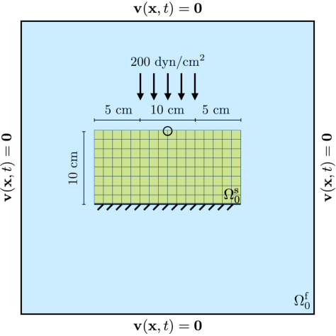
We compress a rectangular block to demonstrate a hyperelastic material response under plane strain. The computational domain is $\Omega=[0,L]^{2}$, with $L=40\,\text{cm}$. A downward uniaxial traction is loaded in the center of the top of the block. Zero horizontal and vertical displacements are respectively applied to the top and bottom boundaries of the block and all other boundaries have zero traction. This test was introduced by Reese et al. [46] to test a stabilization technique for low-order finite elements. Fig. 4 provides a schematic of this test case. A shear modulus of $G=80.194\,\frac{\text{dyn}}{\text{cm}^{2}}$ is used for the incompressible neo-Hookean hyperelastic material, and the downward traction is set to $200\,\frac{\text{dyn}}{\text{cm}^{2}}$. The load time is $T_{\text{l}}=100\,\text{s}$, and the final time is $T_{\text{f}}=500\,\text{s}$. An additional damping is set to $\eta=4.0097\,\frac{\text{g}}{\text{s}}$. To verify the correspondence to benchmark FE results, material failure (i.e., bond breakage) is not allowed.

Fig. 5 illustrates the material body after the deformation along with pointwise values of the non-local Jacobian determinant $J$, which is evaluated from the non-local deformation gradient tensor. Fig. 6 shows the vertical displacements of the top center material point, highlighted in Fig. 4, for various numerical Poisson’s ratios $\nu_{\mathrm{stab}}$ and peridynamic horizon sizes $\epsilon$ under grid refinement. The maximum displacement of the point obtained using IPD method is in excellent agreement with that obtained using the standard FE method, and it converges under grid refinement to approximately $3.92\,\text{cm}$. The maximum displacement of the point of interest is relatively small (between $2.25\,\text{cm}$ and $3.30\,\text{cm}$) at low grid resolutions if a larger value of $\nu_{\mathrm{stab}}=0.49995$ is used. In the computational mechanics literature, this issue is referred to as volumetric locking and can occur with large values of the volumetric penalty parameters. Note that $\kappa_{\mathrm{stab}}\rightarrow\infty$ as $\nu_{\mathrm{stab}}\rightarrow 0.5$. Under grid refinement, we ultimately recover accurate deformations for fixed finite values of $\kappa_{\text{stab}}$, as in standard methods for nearly incompressible elasticity.

Fig. 7 shows the volume change observed under deformation for different grid spacings. If $\nu_{\mathrm{stab}}$ is small, slight volumetric changes occur (between $0.3\%$ and $2.7\%$) under loading. This volume change becomes negligible (up to $0.001\%$) when larger values of $\nu_{\mathrm{stab}}\geq 0.4$ are used. This is also clear in Fig. 5. IPD results agree with results obtained using IFED, with both methods exhibiting similar volume changes that range between $0.0004\%$ and $2.1\%$. Under grid refinement, negligible spurious volume changes or locking occurs in all IPD simulations. In addition, relatively consistent results are obtained for all choices of the PD horizon sizes considered in the tests.

Cook’s membrane [47], which is another widely used plane strain problem, is used to demonstrate the hyperelastic material response under bending and shearing. The computational domain is $\Omega=[0,L]^{2}$, with $L=40\,\text{cm}$. Zero displacement is imposed on the left boundary of the structure, and an upward traction of $6.25\,\frac{\text{dyn}}{\text{cm}^{2}}$ is applied to the right boundary. Otherwise, stress-free boundary conditions are assumed. Fig. 8 provides a schematic of this test case. A shear modulus of $G=83.3333\,\frac{\text{dyn}}{\text{cm}^{2}}$ is used for the incompressible hyperelastic material. The load time is $T_{\text{l}}=20\,\text{s}$, the final time is $T_{\text{f}}=50\,\text{s}$, and the damping parameter is set to $\eta=4.16667\,\frac{\text{g}}{\text{s}}$. We focus on the vertical displacements of the top-right corner of the membrane to assess convergence. To impose the same volume fraction at each material point in the NOSB-PD formulation, we use a stair-step representation of the immersed membrane. Consequently, the horizon size needs to be large enough ($\epsilon\geq\sqrt{2}\Delta X$) to ensure adequate bond connectivity throughout the material. Bond breakage is not considered for this problem as well.

Fig. 9 shows the plane sheet after the deformation along with pointwise values of the non-local Jacobian determinant of non-local deformation gradient tensor at each material point. Fig. 10 shows the $y$-displacement of the top-right corner in Fig. 8 at the steady states for various numerical Poisson’s ratios $\nu_{\mathrm{stab}}$ and PD horizon sizes $\epsilon$ under grid refinement. Fig. 10 shows that the displacements obtained using the IPD method are comparable to those obtained using the classical FE method, and that they converge under grid refinement to approximately $0.67\,\text{cm}$. With $\nu_{\mathrm{stab}}=0.49995$, a larger volumetric penalty causes volumetric locking, which results in smaller displacements when low mesh resolutions are used in the simulations. However, under grid refinement, we ultimately recover accurate deformations for fixed finite values of numerical bulk modulus, as in classical methods for nearly incompressible elasticity.

Fig. 11 shows volume changes observed under deformation for different grid spacings. With smaller values of $\nu_{\mathrm{stab}}$, slight volume changes (between $0.6\%$ and $5.3\%$) are observed under loading. The volume change becomes negligible (up to $0.0005\%$) when larger values of $\nu_{\mathrm{stab}}\geq 0.4$ are used. The volume change using IPD is comparable to the results obtained using IFED, which is between $0.000021\%$ and $0.1\%$. We can expect negligible volume leaking or locking under grid refinement in all IPD simulations. In addition, relatively consistent results are obtained for all considered choices of the PD horizon size.

We use a three-dimensional beam under torsion to investigate three dimensional hyperelastic material responses. This benchmark is based on a test suggested by Bonet et al. [70] and later modified by Vadala-Roth et al. [49] to use with the IFED method. The computational domain is the cube $\Omega=[0,L]^{3}$, with $L=9\,\text{cm}$. One side of the beam is fixed in place, and a torsion is applied to the opposite end through displacement boundary conditions. Fig. 12 provides a schematic of the test case. The right surface is rotated by the linear function $\theta(t)$ from $0$ to $\theta_{T_{\text{f}}}=2.5\pi$ in time. The maximum angle of rotation is achieved at $T_{\text{l}}=0.4T_{\text{f}}$, with $T_{\text{f}}=5\,\text{s}$. All other surfaces have zero traction boundary conditions. Material damage and failure are not considered.

We use the modified Mooney-Rivlin material model [49]

in which $c_{1}$ and $c_{2}$ are material parameters, $I_{1}=\text{tr}\left(\mathbb{C}\right)$, and $I_{2}=\text{tr}\left(\mathbb{C}\right)^{2}-\text{tr}\left(\mathbb{C}^{2}\right)$. The material parameters are set to $c_{1}=c_{2}=9000\,\frac{\text{dyn}}{\text{cm}^{2}}$, and $G=\left(c_{1}+c_{2}\right)$ is used to determine the numerical bulk modulus. The density and viscosity of the surrounding fluid are set to $\rho=1.0\,\frac{\text{g}}{\text{cm}^{3}}$ and $\mu=0.04\,\frac{\text{dyn$\cdot$s}}{\text{cm}^{2}}$, respectively. This larger value of viscosity compared to the previous benchmarks is used to accelerate reaching the steady state.

Overall deformations and volume conservation using the numerical Poisson’s ratio of $\nu_{\text{stab}}=0.4$ in Sec. 4.1.1 and Sec. 4.1.2 are consistent with the classical elasticity results under grid refinement. In general, a larger value of numerical bulk modulus requires a smaller time step size. For the remainder of the IPD simulations presented herein, we only consider two fixed numerical Poisson’s ratios; $\nu_{\text{stab}}=0.4$ for nearly incompressible hyperelastic material models and $\nu_{\text{stab}}=-1.0$ for comparison tests.

Fig. 13 illustrates the deformations of the beam under torsion along with the Jacobian determinant of the non-local deformation gradient tensor at each material point. Fig. 14(a) shows the maximum displacement of the center of the top surface in Fig. 12 at the steady states for various sizes of $\epsilon$ under grid refinement. The displacements using IPD are comparable to the classical FE results and converge under grid refinement to a value of approximately $0.27\,\text{cm}$. Fig. 14(b) shows the volume change of the beam for different numbers of the solid DoF, ranging from $0.13\%$ to $7.41\%$. Volume changes obtained using the IFED method are between $0.16\%$ and $11\%$, which are comparable to the IPD simulations.

This benchmark examines deformations of an elastic band that are driven by fluid forces themselves. The deformations of the elastic band are simulated under fluid pressure loading. The computational domain is $\Omega=[0,2L]\times[0,L]$, with $L=1\,\mathrm{cm}$. Fluid traction boundary conditions are imposed on the boundaries of the computational domain as $\bm{\mathrm{\bbsigma}}^{\text{f}}(\bm{\mathrm{x}},t)\bm{n}(\bm{\mathrm{x}})=\bm{h}(t)$ and $\bm{\mathrm{\bbsigma}}^{\text{f}}(\bm{\mathrm{x}},t)\bm{n}(\bm{\mathrm{x}})=-\bm{h}(t)$ on the left and right, respectively, in which $\bm{\mathrm{\bbsigma}}^{\text{f}}$ is the fluid stress tensor and $\bm{h}(t)=\left(10\sin\left(\frac{\pi t}{2T_{\text{l}}}\right),0\right)\,\frac{\mathrm{dyn}}{\mathrm{cm}^{2}}$ when $t<T_{\text{l}}$ and $\bm{h}(t)=\left(10,0\right)\,\frac{\mathrm{dyn}}{\mathrm{cm}^{2}}$ otherwise. The load time is $T_{\text{l}}=5\,\mathrm{s}$. Zero fluid velocity conditions are applied to the top and bottom boundaries of the computational domain. Different from the previous benchmarks, the difference in pressure across the computational domain causes the deformations of the elastic band. Both top and bottom surfaces of the elastic band are attached to fixed blocks. The stationary blocks serve to block the fluid flow between the wall and the flexible band. Fig. 15 provides a schematic of this test case. We measure the maximum displacement of the point of interest, the encircled point in Fig. 15, at $T_{\text{f}}=15\,\mathrm{s}$. A shear modulus of $G=200\,\frac{\mathrm{dyn}}{\mathrm{cm}^{2}}$ is used for the nearly incompressible neo-Hookean material model. Damage and failure of the elastic band are not allowed. An additional damping force in the structure is used with $\eta=10\,\frac{\text{g}}{\text{s}}$, to accelerate reaching steady state.

Fig. 16 shows the deformations of the elastic band under pressure loading at steady state. Fig. 17(a) shows the maximum horizontal displacement of the point of interest in Fig. 15 at the steady states for different choices of the PD horizon sizes under grid refinement, which is approximately $0.17\,\text{cm}$. Except for $\epsilon=1.015\Delta X$, the results obtained using the IPD method are comparable to FE results. The absence of a diagonal connectivity in the immersed structure with $\epsilon=1.015\Delta X$ causes a lack of resistance to this type of bending. Fig. 17(b) shows the volume change of the band for different numbers of the solid DoF. We observe slight volume changes with smaller values of solid DoF, however, these are resolved under grid refinement. The volume conservation achieved by the IPD method (between $0.015\%$ and $1.2\%$) is comparable to the results generated by the IFED method (between $0.0015\%$ and $2.1\%$).

To investigate nontrivial fluid dynamics in this benchmark, we test the transient behavior of a dynamic version of the elastic band. Instead of gradually applying the fluid traction as the static problem, fluid traction conditions on the boundaries of the computational domain are set to $\bm{\mathrm{\bbsigma}}^{\text{f}}(\bm{\mathrm{x}},t)\bm{n}(\bm{\mathrm{x}})=\bm{h}(t)$, in which $\bm{h}(t)=\left(-10,0\right)\,\frac{\mathrm{dyn}}{\mathrm{cm}^{2}}$ and $\bm{h}(t)=\left(10,0\right)\,\frac{\mathrm{dyn}}{\mathrm{cm}^{2}}$ on the left and right, respectively. The final simulation time is set to $T_{\text{f}}=10\ \mathrm{s}$. Otherwise, we fix the rest of the test parameters as in the static problem, with no damping.

Fig. 18 shows the structural deformations of the band along with the Eulerian velocity field and the values of Jacobian of the non-local deformation tensor. Fig. 19 shows the transient behavior of the elastic band against time for various numerical Poisson’s ratios $\nu_{\text{stab}}$ and peridynamic horizon sizes $\epsilon$ under grid refinement. Fig. 20 shows the volume change of the band under deformation for different choices of $\nu_{\text{stab}}$ and $\epsilon$. The total volume change decreases under grid refinement as in the static case, and the range is comparable to the static case as well. With a larger value of the numerical bulk modulus, the volume change noticeably decreases. Fig. 21(a) and Fig. 21(b) show that the maximum displacements of the oscillations and time to reach the maximum displacements converge under grid refinement. Fig. 22 shows the upper envelops of the oscillations for different choices of $\epsilon$ under grid refinement.

This benchmark considers dynamic material deformations and fracture of the elastic band under fluid-driven forces. In this benchmark, the critical bond stretch is set to $s_{\text{c}}=4.5$ to demonstrate the effectiveness of simulating crack initiation and propagation using the IPD method. In general, the critical bond stretch of a material must be experimentally determined. The critical bond stretch $s_{\text{c}}$ used here is determined based on preliminary simulations. The pressure loading is three times larger than the value used in Sec. 4.1.4 on each side; $\bm{\mathrm{\bbsigma}}^{\text{f}}(\bm{\mathrm{x}},t)\bm{n}(\bm{\mathrm{x}})=\bm{h}(t)$, in which $\bm{h}(t)=\left(-30,0\right)\,\frac{\mathrm{dyn}}{\mathrm{cm}^{2}}$ and $\bm{h}(t)=\left(30,0\right)\,\frac{\mathrm{dyn}}{\mathrm{cm}^{2}}$ on the left and right, respectively. The final simulation time is set to $T_{\text{f}}=0.25\,\mathrm{s}$. Otherwise, we use the same parameters as the non-failure case of the dynamic elastic band benchmark. The horizon size is set to $\epsilon=3.015\Delta X$, as suggested in the PD literature [54].

Fig. 23 shows the crack nucleation and propagation of the dynamic version of the elastic band benchmark with an Eulerian velocity field. The crack formulation is initiated near the junctions between the fixed blocks and the band, and the band gets entirely detached from the block when the bonds exceed the critical bond stretch $s_{\text{c}}$. Fig. 24(a) shows the horizontal displacements of the point of interest, highlighted in Fig. 15, for different grid spacings. Fig. 24(b) shows the local damage growth at the top left corner of the detached band during the failure process under grid refinement.

We next consider the dynamics of an elastic band with a pre-existing crack. A notch is placed on the center-right of the band with the length of $0.05\,\mathrm{cm}$. The pressure loading is set to $\bm{\mathrm{\bbsigma}}^{\text{f}}(\bm{\mathrm{x}},t)\bm{n}(\bm{\mathrm{x}})=\bm{h}(t)$, in which $\bm{h}(t)=\left(-20,0\right)\,\frac{\mathrm{dyn}}{\mathrm{cm}^{2}}$ and $\bm{h}(t)=\left(20,0\right)\,\frac{\mathrm{dyn}}{\mathrm{cm}^{2}}$ on the left and right, respectively, with a zero loading time. In this benchmark, the critical bond stretch is set to $s_{\text{c}}=4.5$ based on preliminary tests. Otherwise, we use the same parameters as the non-failure case of the dynamic elastic band benchmark. To obtain symmetric fracture in the middle of the band, we use even numbers of Lagrangian points in the vertical direction of the elastic band. Fig. 25 provides a schematic of this test case. The horizon size is set to $\epsilon=3.015\Delta X$, as suggested in the PD literature [54]. The final simulation time is set to $T_{\text{f}}=0.3\,\mathrm{s}$.

Fig. 26 shows the dynamic deformation and failure process of the elastic band along with the damage parameter $\varphi$ and Eulerian velocity vectors. The band undergoes a large deformation before the crack propagates, and it ultimately breaks the bond connectivity and completely ruptures. Fig. 27(a) shows the vertical displacements of the point $A$ in Fig. 26 under grid refinement, and Fig. 27(b) shows horizontal displacements of the point $A$ under grid refinement. Fig. 28 shows the local damage growth at the point of interest $B$ during the failure process under grid refinement.

References

- [1] A. A. Griffith, The phenomena of rupture and flow in solids, Philosophical Transactions of the Royal Society of London. Series A 221 (582-593) (1921) 163–198.
- [2] A. Hillerborg, M. Modéer, P.-E. Petersson, Analysis of crack formation and crack growth in concrete by means of fracture mechanics and finite elements, Cement and Concrete Research 6 (6) (1976) 773–781.
- [3] N. Moës, J. Dolbow, T. Belytschko, A finite element method for crack growth without remeshing, International Journal for Numerical Methods in Engineering 46 (1) (1999) 131–150.
- [4] N. Sukumar, J. E. Dolbow, N. Moës, Extended finite element method in computational fracture mechanics: a retrospective examination, International Journal of Fracture 196 (1) (2015) 189–206.
- [5] S. A. Silling, Reformulation of elasticity theory for discontinuities and long-range forces, Journal of the Mechanics and Physics of Solids 48 (1) (2000) 175–209.
- [6] W. Gerstle, N. Sau, S. Silling, Peridynamic modeling of plain and reinforced concrete structures, 18th International Conference on Structural Mechanics in Reactor Technology (2005) 54–68.
- [7] J. Trageser, P. Seleson, Bond-based peridynamics: a tale of two poisson’s ratios, Journal of Peridynamics and Nonlocal Modeling 2 (3) (2020) 278–288.
- [8] S. A. Silling, M. Epton, O. Weckner, J. Xu, E. Askari, Peridynamic states and constitutive modeling, Journal of Elasticity 88 (2) (2007) 151–184.
- [9] T. L. Warren, S. A. Silling, A. Askari, O. Weckner, M. A. Epton, J. Xu, A non-ordinary state-based peridynamic method to model solid material deformation and fracture, International Journal of Solids and Structures 46 (5) (2009) 1186–1195.
- [10] B. E. Griffith, N. A. Patankar, Immersed methods for fluid–structure interaction, Annual Review of Fluid Mechanics 52 (2020) 421–448.
- [11] M. Behzadinasab, G. Moutsanidis, N. Trask, J. T. Foster, Y. Bazilevs, Coupling of iga and peridynamics for air-blast fluid-structure interaction using an immersed approach, Forces in Mechanics 4 (2021) 100045.
- [12] S. Shende, M. Behzadinasab, G. Moutsanidis, Y. Bazilevs, Simulating air blast on concrete structures using the volumetric penalty coupling of isogeometric analysis and peridynamics, Mathematical Models and Methods in Applied Sciences 32 (12) (2022) 2477–2496.
- [13] F. Dalla Barba, F. Picano, A novel approach for direct numerical simulation of hydraulic fracture problems, Flow, Turbulence and Combustion 105 (2) (2020) 335–357.
- [14] Y. Gao, S. Oterkus, Fluid-elastic structure interaction simulation by using ordinary state-based peridynamics and peridynamic differential operator, Engineering Analysis with Boundary Elements 121 (2020) 126–142.
- [15] Y. Zhang, S. Haeri, G. Pan, Y. Zhang, Strongly coupled peridynamic and lattice boltzmann models using immersed boundary method for flow-induced structural deformation and fracture, Journal of Computational Physics 435 (2021) 110267.
- [16] F. Dalla Barba, M. Zaccariotto, U. Galvanetto, F. Picano, 3d fluid–structure interaction with fracturing: A new method with applications, Computer Methods in Applied Mechanics and Engineering 398 (2022) 115210.
- [17] C. S. Peskin, The immersed boundary method, Acta Numerica 11 (2002) 479–517.
- [18] C. S. Peskin, Flow patterns around heart valves: a numerical method, Journal of Computational Physics 10 (2) (1972) 252–271.
- [19] C. S. Peskin, Numerical analysis of blood flow in the heart, Journal of Computational Physics 25 (3) (1977) 220–252.
- [20] C. S. Peskin, D. M. McQueen, A three-dimensional computational method for blood flow in the heart i. immersed elastic fibers in a viscous incompressible fluid, Journal of Computational Physics 81 (2) (1989) 372–405.
- [21] D. M. McQueen, C. S. Peskin, A three-dimensional computational method for blood flow in the heart. ii. contractile fibers, Journal of Computational Physics 82 (2) (1989) 289–297.
- [22] D. M. McQueen, C. S. Peskin, A three-dimensional computer model of the human heart for studying cardiac fluid dynamics, Computer Graphics 34 (1) (2000) 56–60.
- [23] D. M. McQueen, C. S. Peskin, Heart simulation by an immersed boundary method with formal second-order accuracy and reduced numerical viscosity, in: Mechanics for a New Mellennium, Kluwer Academic Publishers, 2002, pp. 429–444.
- [24] B. E. Griffith, X. Luo, D. M. McQueen, C. S. Peskin, Simulating the fluid dynamics of natural and prosthetic heart valves using the immersed boundary method, International Journal of Applied Mechanics 01 (01) (2009) 137–177.
- [25] B. E. Griffith, Immersed boundary model of aortic heart valve dynamics with physiological driving and loading conditions, International Journal for Numerical Methods in Biomedical Engineering 28 (3) (2012) 317–345.
- [26] J. H. Lee, A. D. Rygg, E. M. Kolahdouz, S. Rossi, S. M. Retta, N. Duraiswamy, L. N. Scotten, B. A. Craven, B. E. Griffith, Fluid–structure interaction models of bioprosthetic heart valve dynamics in an experimental pulse duplicator, Annals of Biomedical Engineering 48 (5) (2020) 1475–1490.
- [27] J. H. Lee, L. N. Scotten, R. Hunt, T. G. Caranasos, J. P. Vavalle, B. E. Griffith, Bioprosthetic aortic valve diameter and thickness are directly related to leaflet fluttering: Results from a combined experimental and computational modeling study, JTCVS Open 6 (2021) 60–81.
- [28] Y. J. Choi, V. Vedula, R. Mittal, Computational study of the dynamics of a bileaflet mechanical heart valve in the mitral position, Annals of Biomedical Engineering 42 (8) (2014) 1668–1680.
- [29] S. Bailoor, J.-H. Seo, L. P. Dasi, S. Schena, R. Mittal, A computational study of the hemodynamics of bioprosthetic aortic valves with reduced leaflet motion, Journal of Biomechanics 120 (2021) 110350.
- [30] E. M. Kolahdouz, A. P. S. Bhalla, B. A. Craven, B. E. Griffith, An immersed interface method for discrete surfaces, Journal of Computational Physics 400 (2020) 108854.
- [31] W. Kou, A. P. S. Bhalla, B. E. Griffith, J. E. Pandolfino, P. J. Kahrilas, N. A. Patankar, A fully resolved active musculo-mechanical model for esophageal transport, Journal of Computational Physics 298 (2015) 446–465.
- [32] W. Kou, B. E. Griffith, J. E. Pandolfino, P. J. Kahrilas, N. A. Patankar, A continuum mechanics-based musculo-mechanical model for esophageal transport, Journal of Computational Physics 348 (2017) 433–459.
- [33] A. P. S. Bhalla, B. E. Griffith, N. A. Patankar, A forced damped oscillation framework for undulatory swimming provides new insights into how propulsion arises in active and passive swimming, PLoS Computational Biology 9 (6) (2013) e1003097.
- [34] A. P. S. Bhalla, R. Bale, B. E. Griffith, N. A. Patankar, A unified mathematical framework and an adaptive numerical method for fluid–structure interaction with rigid, deforming, and elastic bodies, Journal of Computational Physics 250 (2013) 446–476.
- [35] G. Herschlag, L. Miller, Reynolds number limits for jet propulsion: A numerical study of simplified jellyfish, Journal of Theoretical Biology 285 (1) (2011) 84–95.
- [36] S. Kern, P. Koumoutsakos, Simulations of optimized anguilliform swimming, Journal of Experimental Biology 209 (24) (2006) 4841–4857.
- [37] I. Borazjani, L. Ge, F. Sotiropoulos, Curvilinear immersed boundary method for simulating fluid structure interaction with complex 3d rigid bodies, Journal of Computational Physics 227 (16) (2008) 7587–7620.
- [38] I. Borazjani, F. Sotiropoulos, Numerical investigation of the hydrodynamics of carangiform swimming in the transitional and inertial flow regimes, Journal of Experimental Biology 211 (10) (2008) 1541–1558.
- [39] A. Santhanakrishnan, S. Jones, W. Dickson, M. Peek, V. Kasoju, M. Dickinson, L. Miller, Flow structure and force generation on flapping wings at low reynolds numbers relevant to the flight of tiny insects, Fluids 3 (3) (2018) 45.
- [40] Z. J. Wang, Dissecting insect flight, Annual Review of Fluid Mechanics 37 (1) (2005) 183–210.
- [41] B. E. Griffith, X. Luo, Hybrid finite difference/finite element immersed boundary method, International Journal for Numerical Methods in Biomedical Engineering 33 (12) (2017) e2888.
- [42] D. Boffi, L. Gastaldi, L. Heltai, C. S. Peskin, On the hyper-elastic formulation of the immersed boundary method, Computer Methods in Applied Mechanics and Engineering 197 (25) (2008) 2210–2231.
- [43] L. Zhang, A. Gerstenberger, X. Wang, W. K. Liu, Immersed finite element method, Computer Methods in Applied Mechanics and Engineering 193 (21) (2004) 2051–2067.
- [44] D. Wells, B. Vadala-Roth, J. H. Lee, B. E. Griffith, A nodal immersed finite element-finite difference method (2021). arXiv:2111.09958.
- [45] P. Diehl, R. Lipton, T. Wick, M. Tyagi, A comparative review of peridynamics and phase-field models for engineering fracture mechanics, Computational Mechanics 69 (6) (2022) 1259–1293.
- [46] S. Reese, M. Küssner, B. D. Reddy, A new stabilization technique for finite elements in non-linear elasticity, International Journal for Numerical Methods in Engineering 44 (11) (1999) 1617–1652.
- [47] R. D. Cook, Improved two-dimensional finite element, Journal of the Structural Division 100 (9) (1974) 1851–1863.
- [48] J. Bonet, R. D. Wood, Nonlinear Continuum Mechanics for Finite Element Analysis, Cambridge University Press, Cambridge, 1997.
- [49] B. Vadala-Roth, S. Acharya, N. A. Patankar, S. Rossi, B. E. Griffith, Stabilization approaches for the hyperelastic immersed boundary method for problems of large-deformation incompressible elasticity, Computer Methods in Applied Mechanics and Engineering 365 (2020) 112978.
- [50] M. Hillman, M. Pasetto, G. Zhou, Generalized reproducing kernel peridynamics: unification of local and non-local meshfree methods, non-local derivative operations, and an arbitrary-order state-based peridynamic formulation, Computational Particle Mechanics 7 (2) (2019) 435–469.
- [51] E. Madenci, E. Oterkus, Peridynamic Theory and Its Applications, Springer, New York, 2014.
- [52] S. A. Silling, E. Askari, A meshfree method based on the peridynamic model of solid mechanics, Computers & Structures 83 (17-18) (2005) 1526–1535.
- [53] J. T. Foster, S. A. Silling, W. Chen, An energy based failure criterion for use with peridynamic states, International Journal for Multiscale Computational Engineering 9 (6) (2011).
- [54] D. Behera, P. Roy, E. Madenci, Peridynamic correspondence model for finite elastic deformation and rupture in neo-hookean materials, International Journal of Non-Linear Mechanics 126 (2020) 103564.
- [55] R. Glowinski, T.-W. Pan, T. Hesla, D. Joseph, A distributed lagrange multiplier/fictitious domain method for particulate flows, International Journal of Multiphase Flow 25 (5) (1999) 755–794.
- [56] N. Patankar, P. Singh, D. Joseph, R. Glowinski, T.-W. Pan, A new formulation of the distributed lagrange multiplier/fictitious domain method for particulate flows, International Journal of Multiphase Flow 26 (9) (2000) 1509–1524.
- [57] R. Glowinski, T. Pan, T. Hesla, D. Joseph, J. Périaux, A fictitious domain approach to the direct numerical simulation of incompressible viscous flow past moving rigid bodies: Application to particulate flow, Journal of Computational Physics 169 (2) (2001) 363–426.
- [58] B. E. Griffith, An accurate and efficient method for the incompressible navier–stokes equations using the projection method as a preconditioner, Journal of Computational Physics 228 (20) (2009) 7565–7595.
- [59] P. Colella, P. R. Woodward, The piecewise parabolic method (PPM) for gas-dynamical simulations, Journal of Computational Physics 54 (1) (1984) 174–201.
- [60] W. Hu, Y. Ha, F. Bobaru, Numerical integration in peridynamics, technical report, University of Nebraska-Lincoln, Department of Mechanical and Materials Engineering (2010).
- [61] P. Seleson, D. J. Littlewood, Numerical tools for improved convergence of meshfree peridynamic discretizations, in: Handbook of Nonlocal Continuum Mechanics for Materials and Structures, Springer International Publishing, 2017, pp. 1–27.
- [62] P. Seleson, M. Parks, On the role of the influence function in the peridynamic theory, International Journal for Multiscale Computational Engineering 9 (6) (2011) 689–706.
- [63] B. E. Griffith, R. D. Hornung, D. M. McQueen, C. S. Peskin, An adaptive, formally second order accurate version of the immersed boundary method, Journal of Computational Physics 223 (1) (2007) 10–49.
- [64] IBAMR: An adaptive and distributed-memory parallel implementation of the immersed boundary method, https://ibamr.github.io/.
- [65] C. S. Peskin, B. F. Printz, Improved volume conservation in the computation of flows with immersed elastic boundaries, Journal of Computational Physics 105 (1) (1993) 33–46.
- [66] B. E. Griffith, On the volume conservation of the immersed boundary method, Communications in Computational Physics 12 (2) (2012) 401–432.
- [67] B. Wang, S. Oterkus, E. Oterkus, Determination of horizon size in state-based peridynamics, Continuum Mechanics and Thermodynamics 35 (3) (2023) 705–728.
- [68] S. A. Silling, R. B. Lehoucq, Convergence of peridynamics to classical elasticity theory, Journal of Elasticity 93 (1) (2008) 13.
- [69] P. Seleson, D. J. Littlewood, Convergence studies in meshfree peridynamic simulations, Computers & Mathematics with Applications 71 (11) (2016) 2432–2448.
- [70] J. Bonet, A. J. Gil, R. Ortigosa, A computational framework for polyconvex large strain elasticity, Computer Methods in Applied Mechanics and Engineering 283 (2015) 1061–1094.
- [71] S. A. Silling, Stability of peridynamic correspondence material models and their particle discretizations, Computer Methods in Applied Mechanics and Engineering 322 (2017) 42–57.
- [72] X. Gu, Q. Zhang, Y. Yu, An effective way to control numerical instability of a nonordinary state-based peridynamic elastic model, Mathematical Problems in Engineering 2017 (2017).
- [73] J. Luo, V. Sundararaghavan, Stress-point method for stabilizing zero-energy modes in non-ordinary state-based peridynamics, International Journal of Solids and Structures 150 (2018) 197–207.
- [74] S. R. Chowdhury, P. Roy, D. Roy, J. Reddy, A modified peridynamics correspondence principle: Removal of zero-energy deformation and other implications, Computer Methods in Applied Mechanics and Engineering 346 (2019) 530–549.
- [75] M. Tupek, R. Radovitzky, An extended constitutive correspondence formulation of peridynamics based on nonlinear bond-strain measures, Journal of the Mechanics and Physics of Solids 65 (2014) 82–92.