Computing a classic index for finite-horizon bandits
Abstract
This paper considers the efficient exact computation of the counterpart of the Gittins index for a finite-horizon discrete-state bandit, which measures for each initial state the average productivity, given by the maximum ratio of expected total discounted reward earned to expected total discounted time expended that can be achieved through a number of successive plays stopping by the given horizon. Besides characterizing optimal policies for the finite-horizon one-armed bandit problem, such an index provides a suboptimal heuristic index rule for the intractable finite-horizon multiarmed bandit problem, which represents the natural extension of the Gittins index rule (optimal in the infinite-horizon case). Although such a finite-horizon index was introduced in classic work in the 1950s, investigation of its efficient exact computation has received scant attention. This paper introduces a recursive adaptive-greedy algorithm using only arithmetic operations that computes the index in (pseudo-)polynomial time in the problem parameters (number of project states and time horizon length). In the special case of a project with limited transitions per state, the complexity is either reduced or depends only on the length of the time horizon. The proposed algorithm is benchmarked in a computational study against the conventional calibration method.
Keywords: dynamic programming, Markov; bandits, finite-horizon; index policies; analysis of algorithms; computational complexity
MSC (2010): 90C15; 60G40; 90C39; 90C40; 91A60; 91B82
1 Introduction
This paper deals with a class of finite-horizon discrete-state bandit problems, whose optimal policy is known to be of index type. In contrast to the existing literature, where such an index is computed approximately via the so-called calibration method, this paper provides an efficient and exact algorithm to compute the index.
1.1 Finite-horizon multiarmed bandits
In the classic finite-horizon multiarmed bandit problem (FHMABP), a decision maker aims to maximize the expected total discounted reward earned from a finite collection of dynamic and stochastic projects, one of which must be engaged at each of a finite number of discrete time periods . Project is modeled as a discrete-time bandit, i.e., a binary-action (active: ; passive: ) Markov decision process (MDP) whose state moves through the discrete (finite or countably infinite) state space . If the project is engaged () at time when it occupies state , it yields an expected active reward and its state evolves to with probability . Otherwise, it neither yields reward (i.e., the passive reward is ) nor changes state. Rewards are discounted with factor , where the term “discounted” is abused to include the undiscounted case .
Decisions as to which project to engage at each time are based on adoption of a scheduling policy , to be drawn from the class of admissible policies, which engage one project at each time before time , and are nonanticipative (with respect to the history of elapsed time periods, states and actions) and possibly randomized.
The FHMABP is to find an admissible policy that maximizes the expected total discounted reward earned. Denoting by the expectation under policy conditioned on the initial joint state being equal to , we can formulate such a problem as
| (1) |
The problem has its roots in the seminal works of Robbins 1952 and Bradt et al. 1956, who focused on the much-studied case where engaging a project corresponds to sampling from a Bernoulli population with unknown success probability, the goal being to maximize the expected number of successes over plays. An MDP formulation is obtained by a Bayesian approach, where a project/population state is its posterior distribution.
The above FHMABP and some of its variants have since drawn extensive research attention, due to their theoretical and practical interest. See, e.g., the monograph by Berry and Fristedt 1985 and references therein. More recently, Caro and Gallien 2007 address a problem extension where projects are to be engaged at each time, motivated by a dynamic assortment problem in the fashion retail industry.
1.2 The average-productivity index policy
Finding an optimal policy for such a problem through numerical solution of its dynamic programming (DP) equations quickly becomes computationally intractable as the time horizon or the projects’ state spaces grow, which has led researchers to investigate a variety of tractable, though suboptimal, heuristic scheduling rules. Simple examples include the “play the winner/switch from a loser” rule (for Bernoulli bandits) and the myopic policy, which engages at each time a project of currently highest expected reward.
Yet, for a special case of (1), the two-armed bandit problem with one arm known — also known as the one-armed bandit problem— where there are two projects and one (the known arm or standard project) has a single state with reward , the structure of optimal policies is well known, being characterized by an index attached to states and times-to-go for the other project (the unknown arm, for which the label is henceforth dropped from the notation). Note that in such a setting, to be used throughout the paper, time is counted backwards, i.e., is the number of remaining periods at which the project can be engaged. It turns out that it is optimal to engage the latter project when it occupies state and periods remain iff , i.e., iff its current index is greater than or equal to the standard project’s reward. Such a result was first established for an undiscounted Bayesian Bernoulli bandit in Bradt et al. 1956. For an overview and extensions see Berry and Fristedt 1985.
An economically insightul alternative representation of such an index is
| (2) |
where the right-hand-side is an optimal-stopping problem, with denoting a stopping-time rule for abandoning the project provided it is engaged at least once starting at with remaining periods. Thus, is an average productivity (AP) index, measuring the maximum rate of expected discounted reward that can be earned per unit of expected discounted time expended by successively engaging the project no more than times starting at .
Besides characterizing optimal policies for the finite-horizon two-armed bandit problem with one arm known, also serves as a dynamic priority index for engaging a project, furnishing a heuristic index policy for the general FHMABP (1) that engages at each time a project of currently highest index value. In the problem variant where at most projects are to be engaged at each time, the resulting index policy engages the project(s) with larger positive index values, if any, up to a maximum of . Such a variant is particularly relevant when observation costs or activity charges are incorporated into the model. Thus, note that it follows immediately from (2) that, if the aforementioned project model is modified to include a charge to be incurred each time the project is engaged, so the active reward is , the corresponding index becomes .
The empirical performance of the index rule based on for the case of two Bernoulli projects with Beta priors is investigated in Ginebra and Clayton 1999, where it is shown to be very close to optimal for small time horizons. In Caro and Gallien 2007, such an index rule is also considered, although the authors introduce and use instead an approximation for based on approximate DP, which is less costly to evaluate.
The index is monotone nondecreasing in the remaining time . Hence, for a project with bounded rewards it has a finite limit as . Bellman 1956 showed that characterizes optimal policies for the infinite-horizon two-armed Bernoulli bandit problem with one arm known and . The resulting index rule was shown in Gittins and Jones 1974 to be optimal for the infinite-horizon multiarmed bandit problem with one project engaged at each time, which has led to being known as the Gittins index.
Although efficient algorithms to compute the Gittins index of a finite-state project are available, the currently lowest time complexity — counting the number of arithmetic operations (AOs) — for a general -state project being (as Gaussian elimination) for the algorithm given in Niño-Mora 2007, the Gittins index of a countably-infinite state project can only be approximated, using the AP index for a large horizon . Wang 1997 shows the rate of convergence of to to be linear for .
In contrast, scant research attention has been given to the efficient computation of the AP index for a general project. The limited previous work, which we review in Section 2, typically focuses on specific models, and either uses DP to obtain approximate index values, or draws on the optimal-stopping representation (2) to obtain exact index values. The latter approach, however, has not yielded an exact index algorithm of general applicability with polynomial time complexity in both the horizon and in the number of states .
A one-pass exact index algorithm with time complexity was presented in Niño-Mora 2005, using the adaptive-greedy restless-bandit index algorithm introduced in Niño-Mora 2001; Niño-Mora 2002. The term “adaptive-greedy” refers to the fact that such an algorithm finds a local maximizer for a certain vector at each step in an adaptive fashion, meaning that such a vector is updated after the step. A recursive version with an improved time complexity, using memory locations, was presented in Niño-Mora 2008, by exploiting the structure of the restless bandit formulation of a finite-horizon bandit.
This paper develops, simplifies, and extends such work, as it does not rely on restless bandit indexation and extends the algorithm’s scope to countably-infinite state projects. For a project with limited transitions per state, the time complexity is reduced to , and in such a case the algorithm is further extended to countably-infinite state projects with an time complexity and an memory complexity. A computational study demonstrates the index algorithm’s practical tractability for moderate-size instances.
For comparison, the paper includes in Section 2.1 an assessment of the complexity of approximate index computation via the conventional calibration method, which solves by DP a collection of finite-horizon optimal stopping problems at a finite grid of -values (from which the approximate index values are taken). The complexity of such a method grows linearly in the grid size , being time and space. Hence, if is taken equal to the number of index values to be evaluated, one obtains time and space complexities of and , as in the exact algorithm proposed herein.
The remainder of the paper is organized as follows. Section 2 reviews previous approaches to the finite-horizon AP index’ computation. Section 3 develops the recursive index algorithm for finite-state projects. Section 4 extends the algorithm’s scope to countably-infinite state projects. Section 5 presents an efficient block implementation (see Dongarra and Eijkhout 2000) of the algorithm, which is necessary for making it useful in practice. Section 6 reports the results of a computational study. Section 7 concludes.
Ancillary material is available in an online supplement.
2 Previous approaches to the AP index computation
Two approaches have been proposed, as discussed below.
2.1 The calibration method for approximate index computation
The first, known as the calibration method, uses DP to obtain approximate index values, adapting to the finite-horizon setting the method in Gittins 1979 for approximate Gittins index calculation, as outlined in Berry and Fristedt 1985. Denoting by the optimal value of the two-armed bandit problem with one arm known, where the unknown project starts at with remaining periods, is the smallest root in of
| (3) |
where if and if . Note that, for a fixed , is recursively characterized by the DP equations
| (4) |
which use the result, first proven in Bradt et al. 1956, that, if the standard project is optimal at any stage, then it is also optimal thereafter.
The calibration method solves such DP equations for a grid of increasing -values , with and , which gives index approximations with the desired degree of accuracy. Table 1 shows an efficient block implementation (see Dongarra and Eijkhout 2000) of the calibration method, where is the matrix , with , and is an -vector of ones. Note that the “max" shown in Table 1 are to be read componentwise. As discussed in Section 5, block implementations achieve economies of scale in computation by rearranging bottleneck calculations as operations on large data blocks. In Table 1, this is achieved with the matrix-update . The required minimization can be carried out using bisection search.
The following result assesses both the time (AOs) and the memory complexities (the latter measuring intermediate floating-point storage locations, i.e., excluding input and output) of the calibration method. Since it appears reasonable to deploy such an approach using a grid contaning a number of -values that is at least as large as the number of index values, i.e., , Proposition 2.1(c) estimates the complexity in the case .
ALGORITHM : Input: Output: ; for to do { note: } end { for }
Proposition 2.1
For an -state project with horizon
- (a)
For a fixed , the for can be computed in time and space.
- (b)
Using a size- grid, the calibration method uses time and space.
- (c)
If , then the calibration method uses time and space.
Proof. (a) Computing involves the subtractions required to obtain for every . For , in order to compute given and , one first computes , which takes AOs. Multiplying the result by , adding it to , and then subtracting to determine the “max” takes 3 AOs. Repeating for every takes AOs. The is computed from , which takes 2 additional AOs. Repeating for gives the term. Further, storage of the uses floating-point memory locations.
Parts (b) and (c) follow immediately from parts (a) and (b), respectively.
Note further that the calibration method is immediately parallelizable, as the computations for nonoverlapping ranges of -values can be split among different processors. Hence, its time complexity scales linearly with the number of processors.
2.2 The direct method for exact index computation
In contrast to the calibration method, which is presently the preferred approach, the direct method computes exact index values and is relatively unexplored. It was introduced in Bradt et al. 1956, and has been extended in Berry and Fristedt 1985 to more general discount sequences. The direct method draws on the representation in (2), calling for the solution of the corresponding optimal stopping problems.
In Gittins 1979, such a method is deployed to compute the index for a Bernoulli bandit with Beta priors, with the goal of approximating its Gittins index . Two key results, which reduce the complexity of the optimal stopping problems of concern, and give a recursive index computation, are Corollaries 1 and 2 in that paper.
Proposition 2.2 (Corollary 1 in Gittins 1979)
An optimal stopping time for (2) is
| (5) |
Proposition 2.3 (Corollary 2 in Gittins 1979)
In order to solve optimal-stopping problem (2), it suffices to consider stopping times of the form
| (6) |
where the “min” of an empty set is taken to be .
The direct method outlined in Gittins 1979 draws on Proposition 2.2, reducing optimal-stopping problem (2) to the one-dimensional continuous optimization problem
| (7) |
which corresponds to formula (11) in that paper.
However, in Gittins 1979 it is not discussed how to solve exactly the right-hand-side optimization problem over in (7), although in the review of such an approach in Gittins 1989 it appears to be suggested to use a grid of -values and interpolation for such a purpose, which would render the method approximate rather than exact.
Varaiya et al. 1985 gives a Gittins-index algorithm that exploits the corresponding result in Proposition 2.2 for the Gittins index, as stated in the lemma on p. 154 of Gittins 1979. The Varaiya et al. (1985) algorithm avoids solving the corresponding continuous optimization problem (7), as it only involves discrete maximizations.
In fact, Proposition 2.2 ensures that the continuous optimization problem in the right-hand-side of (7) can be reduced to the discrete optimization problem
| (8) |
Yet, this observation does not directly yield an adaptive-greedy algorithm for the AP index analogous to that of Varaiya et al. for the Gittins index .
3 Recursive index computation
This section develops the recursive adaptive-greedy index algorithm that is the main contribution of this paper, for a project with a finite number of states.
3.1 Reduction to a modified Gittins index
Let us first prepare the ground for computing a project’s finite-horizon AP index , by showing that such an index can be reduced to a modified Gittins index, which allows use of the adaptive-greedy algorithm available for the latter index to compute the former.
Consider an auxiliary infinite-horizon project, whose state evolves over time periods through the state space , where is the set of controllable states where both actions (active and passive) are allowed, and is the (singleton) set of uncontrollable states where the passive action must be taken, with denoting a terminal absorbing state. Under the active action , the project’s transition probabilities are for and , while its rewards are . Under the passive action , the project remains frozen, its transition probabilities being , while its immediate rewards are . Further, all other transition probabilities are zero.
The idea of forcing a project to be passive in certain states, termed uncontrollabe, was introduced in Niño-Mora 2002 in the setting of restless bandits, where a project’s index is only defined for its controllable states. This is relevant in the present setting, as shown next. Suppose we allow the active action to be taken at the absorbing state in the auxiliary infinite-horizon project described above, with the same dynamics and rewards as the passive action. Let be the corresponding conventional Gittins index, which is defined by
| (9) |
where is a stopping time under which the project is engaged at least once starting at . Now, let be the modified Gittins index of the project with state and uncontrollable state , which is defined only for its controllable states by
| (10) |
Note that, unlike (9), optimal-stopping problem (10) only considers stopping times that idle the project at , i.e., . Such a distinction between the conventional and the modified Gittins index is significant, since in some cases the two may differ. Thus, e.g., for a state with , .
The interest of introducing such an auxiliary project and its modified Gittins index is that the latter is precisely the finite-horizon AP index of concern here.
Proposition 3.1
for .
Proof. The result follows by noting that, under a stopping time for the original project’s state process starting at with remaining periods, the process defined by for has the same (active) dynamics and rewards as that used to define above, and therefore
3.2 Adaptive-greedy index algorithm
The representation in Proposition 3.1 of the finite-horizon index as the modified Gittins index of an infinite-horizon project allows us to use available algorithms for the latter type of index to compute the former. Note, however, that the classic adaptive-greedy Gittins-index algorithm of Varaiya et al. 1985 should not be directly used, since it computes the conventional Gittins index which, as argued above, can differ from the modified Gittins index . Also, such an algorithm does not exploit special structure.
We will use instead an extension of such an algorithm introduced in Niño-Mora 2001 for restless bandits, and further extended in Niño-Mora 2002 to a wider setting. A key feature of such an algorithm is that it exploits special structure to reduce the computational burden. Rather than describing the algorithm in full generality, for which the reader is referred to the aforementioned papers, we present it next as it applies to the model of concern.
To prepare the ground, we start by introducing two measures to evaluate a stopping-time rule for the project (refer to the discussion in Section 3.1): a reward measure
giving the expected total discounted reward earned starting at with remaining periods; and the work measure
giving the corresponding expected total discounted time that the project is active.
Due to the optimality of deterministic Markov policies for finite-state and -action MDPs, it suffices to consider stopping times given by a continuation (or active) set , consisting of those controllable states at which the project is active under . We will find it convenient to represent each such continuation set in a more explicit fashion, writing
| (11) |
where is the continuation set when periods remain. Thus, the stopping rule having continuation set engages the original project in state when periods remain (or the modified project in state ) iff . We will write and to denote the reward measures and work measures, respectively, under such a stopping rule.
Further, we will use the modified reward and work measures defined by
| (12) |
respectively, along with the productivity rate measure defined by
| (13) |
Now, the classic result referred to in Section 1, whereby if it is optimal to stop the project when periods remain, then it is also optimal to do so when less periods remain, allows us to restrict the continuation sets that need be considered to those consistent with such a property, which constitute the continuation-set family
| (14) |
We are now ready to present the adaptive-greedy index algorithm , which is shown in Table 2. Such an algorithm builds up in steps (note that is the number of controllable states) an increasing nested chain of adjacent continuation sets (i.e., differing by one state) in connecting the empty set to the full controllable state space, proceeding at each step in a greedy fashion. Thus, once the continuation set has been constructed, the next continuation set is obtained by adding to a controllable state that maximizes the productivity rate over augmented states for which the next active set remains in , i.e., with . Ties are broken arbitrarily.
Note that in Table 2 we write, for notational convenience, as . The algorithm’s output consists of an augmented-state sequence spanning , along with a corresponding nonincreasing sequence of index values .
ALGORITHM : Output: for to do pick ; ; end { for }
We next use the definition of in (14) to obtain the more explicit reformulation of algorithm shown in Table 3, breaking down the choice at step of the augmented state to be added to the current continuation set .
ALGORITHM Output: ; for to do { note: } pick ; ; ; end { for }
3.3 Reward and work measure recursions
The above algorithms do not specify how to compute the required modified reward and work measures (see (13)) to calculate productivity rates . This section presents recursions that will be used for such a purpose in the next section.
Let be a continuation set in . Note first that, from the stopping-rule interpretation of , it is clear that the reward measure does not depend on for , which allows us to write as for , while . Further, the definition of modified reward measure in (12) ensures that it does not depend on for , which allows us to write as for , while .
In the following result, part (a) shows how to recursively evaluate modified reward measures for a fixed . The remaining parts show how to evaluate the modified reward measure for an augmented continuation set, , based on knowledge of the . While the base continuation set is written as , the reduction discussed in the previous paragraph should be taken into account, as it plays a key role in the proof. Also, note that .
Lemma 3.2
For , :
- (a)
- (b)
, for .
- (c)
, for .
- (d)
, for , .
Proof. (a) This part follows immediately from the definition of in (12) and the project’s dynamics and rewards under the stopping rule induced by continuation set .
(b) The result follows from
(c) The result, which draws on part (a), follows from
(d) The result, which also draws on part (a), follows from
The following result is the counterpart of Lemma 3.2 for modified work measures . It follows immediately from the above by taking , and hence we omit its proof.
Lemma 3.3
For , :
- (a)
- (b)
, for ,
- (c)
, for ;
- (d)
, for ,
3.4 A -stage recursive adaptive-greedy index algorithm
This section draws on the above results to reformulate the one-pass adaptive-greedy index algorithm in Table 3 into a -stage recursive adaptive-greedy (RAG) algorithm.
ALGORITHM Input: Output: ; ; ; ; repeat { note: } ; pick if then ; ; ; if then else if then ; else { } end { if } end { if } ; until { repeat }
Consider the algorithm’s th stage, , for a given remaining time , which is shown in Table 4, where . The input to consists of (i) the index values for smaller horizons ; and (ii) sequences labeled by (with being part of the input) of augmented states , and of modified work and reward measures and from the previous stage. The output of gives the input to the next stage.
Algorithm performs steps, labeled by , to build up the first continuation sets of those constructed by algorithm in Table 3, using its input to avoid redundant computations. Note that , , and for . As before, in the algorithm’s notation and stand for and , respectively. For a continuation set as above, we write , with . Note that .
The key insight on which the design of algorithm is based is that the successive continuation sets , for , corresponding to the constructed by algorithm , are precisely those constructed by the previous stage’s algorithm, . Exploiting such an insight allows us to simplify algorithm in Table 3, as follows. Consider step of algorithm , which corresponds to step of . Such a step identifies the augmented state that will be added to the current continuation set to obtain the next one, , with the index of augmented state being then given by . Such a maximization of is now broken down into two parts: that for horizon , and that for smaller horizons , with the first being the only one that requires actual computations, since the second was already evaluated in previous stages, having as maximizing argument , with . Algorithm stops as soon as , i.e., , performing steps.
As the step counter advances, algorithm constructs the required modified work and reward measures and using the recursions obtained in Section 3.3. The update formulae to use depend on the value of . Three cases need to be considered. In the first case, , we use Lemmas 3.2(b) and 3.3(b) to conclude that
In the second case, , Lemmas 3.2(c) and 3.3(c) yield that, with :
| (15) |
Finally, in the third case, , we use Lemmas 3.2(d) and 3.3(d) to obtain
| (16) |
where again . Such recursions are initialized by setting and .
The above applies to a stage . As for the initial stage , the required quantities are obtained by setting , , and .
The following result establishes the validity of the resulting -stage index algorithm RAG, which successively runs the stages , , …, , and assesses its time and memory complexity.
Theorem 3.4
Algorithm RAG computes all index values in time and space.
Proof. The result that algorithm RAG computes index is already proven by the above discussion. Regarding the time complexity, let us focus on a given stage (with ), i.e., on algorithm . The description of as given in Table 4 shows that the bulk of the computational work corresponds to the update in (16), which entails
AOs. Adding up such an upper bound over steps gives for stage . Then, adding up over stages gives the upper bound .
As for memory, the bulk of the storage requirements at the last, more expensive stage , corresponds to quantities , and , with , which use floating-point locations. Since memory can be reused from one stage to the next, this gives the overall memory complexity.
Since index values are computed, Theorem 3.4 ensures that the average complexity per index value of algorithm RAG is time and space.
3.5 Limited transitions per state: index algorithm
The time complexity of the RAG index algorithm holds for a general project. Yet, in many models arising in applications, the state transition probability matrix is sparse, as only a limited number of states, which remains fixed as the total number of states varies, can be reached from any given state. Namely, the following condition holds.
Assumption 3.5
For every state , .
In such cases, the time complexity of the RAG algorithm given in the previous section is reduced by an order of magnitude in the total number of states.
Proposition 3.6
Under Assumption 3.5, the RAG algorithm computes all index values in time.
4 Computing the relevant index values of a countable-state project
For a finite-state project, the RAG algorithm computes index values for every intermediate horizon and state combination. Yet, to deploy the resulting priority-index policy in a particular instance of the FHMABP (1), the index of each project need not be evaluated at each such pair, but only at the typically smaller subset of relevant , i.e., those that can be reached from the initial state within the allotted time. Even for a project with a countably infinite state space, provided it satisfies Assumption 3.5 — such as the classic Bernoulli bandit with Beta priors, for which — the set of relevant pairs is finite. This section presents a modified version of the RAG algorithm that computes the index values only at such relevant pairs.
Consider a project whose state moves through the countable (finite or infinite) state space , with its transition probabilities satisfying Assumption 3.5. Suppose the project starts at with horizon . Then, the project’s index need be evaluated only at pairs such that: (i) ; and (ii) state belongs to the finite set of states that can be reached within periods starting at . Note that , and that
Let be the finite set of such relevant pairs, and let . Note that contains augmented states .
Consider now an auxiliary finite-state infinite-horizon project, whose state evolves over time periods through the state space , defined as in Section 3.1 but using and in place of and . Now, let be the modified Gittins index of such an auxiliary project, as defined by (10). The interest of introducing such an auxiliary project and its modified Gittins index is, as in Section 3.1, that the latter is precisely the finite-horizon index . The proof of the next result follows along the same lines as that of Proposition 3.1, and is hence omitted.
Proposition 4.1
for .
As in Section 3.2, Proposition 4.1 allows us to obtain the finite set of relevant index values for by running the adaptive-greedy algorithm in Table 2. Yet, note that the definition of active-set family in (14) used in Section 3.2 must be modified in the present setting to .
We can now use the recursionspresented in Section 3.3, along the lines in Section 3.4, to reformulate the one-pass algorithm into a -stage recursive algorithm, which we denote by to emphasize its dependence on the initial project state . Table 5 shows stage of such an algorithm, which we denote by , for .
ALGORITHM Input: Output: ; ; ; ; repeat { note: } pick if then ; ; ; if then else if then else { } end { if } end { if } ; until { repeat }
The next result ensures the validity of the resulting -stage index algorithm , which successively runs the stages , , …, , and assesses its complexity. For the latter purpose, we further assume a quadratic growth rate for in the remaining time , as this is common in applications.
Assumption 4.2
.
Under Assumption 4.2, algorithm computes index values .
Theorem 4.3
Algorithm computes index values in time and space.
Proof. The result that algorithm computes the stated values of index is already proven by the above discussion. Regarding the time complexity, let us focus on a given stage (with ), i.e., on algorithm . The description of as given in Table 5 shows that the computational bottleneck is the update
which entails no more than AOs. Adding up such an upper bound over steps gives no more than for stage . Then, adding up over stages and using Assumption 4.2, gives an upper bound of AOs.
As for memory, the bulk of storage at stage corresponds to the and for , , and . Now, for every , (see Assumption 4.2) floating-point memory locations are needed.
To illustrate, in the case of the Bernoulli bandit model with Beta priors, where the state is a pair giving the parameters of the corresponding posterior Beta distribution, suppose one wants to compute the index values for states that can be reached from a given initial state within periods. For such a model, Assumption 3.5 holds with and, since
Assumption 4.2 also holds, since . Hence, the total number of index values that is computed by algorithm is .
The reader may wonder how the complexity results in Theorem 4.3, as applied to the Bernoulli bandit model with Beta priors, compare with those reported in Gittins 1989, which might appear better at first glance, being AOs and memory. The answer is that both complexity counts cannot be meaningfully compared, for the following reasons: (i) the purpose of the algorithm in Gittins 1979 is to approximate the Gittins index at a single state by , for which only the subset of index values of the form , for and , needs to be evaluated; and (ii) the Gittins algorithm calls for solving a continuous optimization problem of the form (7) at each step, which is not an elementary operation, whereas the RAG algorithm herein performs only arithmetic operations.
5 Block implementation of the RAG index algorithm
This section presents an efficient implementation of the RAG index algorithm. A naive implementation which directly codes the algorithm’s update formulae will be found to be rather slow and inefficient, even for instances with a moderate number of states or horizon. The reason is that the bottleneck computation, which is the update in (16), involves repeated multiplications of large matrices with noncontiguous memory-access patterns, requiring expensive gather and scatter memory operations. Such patterns cause severe inefficiencies in linear algebra algorithms, due to the mismatch between the speeds of processors (fast) and of memory access (slow) in contemporary computers. The main approach to reduce such inefficiencies, exploiting both vectorization and parallelism features of advanced computer architectures, is to design block implementations. These aim to maximize the arithmetic operations performed per memory access, by rearranging bottleneck computations as linear algebra operations on contiguous blocks of data (e.g., matrix-matrix multiplications), thus attaining a sort of economies of scale in computation. See Dongarra and Eijkhout 2000.
ALGORITHM Input: , Output: , ; ; ; ; repeat { note: } ; pick if then ; ; ; ; if then ; end { if } else if then else { } end { if } end { if } ; until { repeat } for do: , ; end { for }
Table 6 presents a block implementation of stage of the RAG algorithm, denoted by . The input to differs from that to in that (i) it takes a matrix of vectors and instead of the and , where and , where corresponds to the continuation sets generated by algorithm ; and (ii) it incorporates vectors and , where and , with being the first continuation set for horizon in algorithm that contains state . The output of algorithm differs accordingly from that of .
6 Computational experiments
This section reports the results of a computational study, based on the author’s Fortran implementations of the algorithms discussed above (which are available for download at http://alum.mit.edu/www/jnimora, under the link “Original software codes"), which benchmarks the actual runtime and memory performance of the proposed RAG algorithm against the calibration method, and fits the measured performance to the theoretical complexity.
6.1 Index computation for finite-state projects
This experiment benchmarks the RAG index algorithm against the calibration method on finite-state projects, measuring actual runtime performance and storage requirements. Recall that Theorem 3.4 establishes an time complexity and an memory complexity for the RAG algorithm on an -state -horizon project, whereas Proposition 2.1(b) shows that the time and memory complexities for the calibration method, when used with a grid of -values, are and , respectively.
The experiment uses the block implementations (see
Sections 2.1 and
5) designed and coded in Fortran by
the author of the calibration
method and the
RAG algorithm.
The codes
were compiled using the latest release
at the time of writing of the Intel Visual Fortran Compiler
Professional Ed. 11.1 (Update 6).
Such implementations use high-performance threaded
routines from the Intel Math Kernel Library for
bottleneck computations (in particular the BLAS Level 3
DGEMM subroutine
for matrix-matrix multiplication), which can harness to a substantial extent
the parallel processing power of the platform employed: an
HP z800 workstation with two quad-core 3.33 GHz
Intel Xeon processors w5590 and 48 GB of memory,
under Windows 7 x64.
Both methods were tested on 20 project instances,
with state-space sizes , and a horizon of .
The transition probability matrix of the -state instance
was obtained by scaling an matrix with pseudorandom
entries, dividing each row by its sum.
Immediate rewards were also drawn from a pseudorandom
distribution.
The discount factor used was .
For each instance, the index values
for and
were evaluated using the RAG algorithm and the
calibration method, the latter for 3, 4, and 5 significant digits of
accuracy (partitioning the unit interval
with a grid of equally-spaced -values, for ).
For each method and
intermediate horizon ,
the wall-clock cumulative runtime to compute the index values
for and was
measured using the Fortran intrinsic subroutine system_clock.
Figure 1 plots the recorded cumulative runtimes (in minutes) versus the number of states for horizon . The gray solid lines shown are polynomial least-squares (LS) fits for the predicted runtimes, of 3rd order for the RAG algorithm, and of 2nd order for the calibration method, corresponding to the theoretical complexities. In the case of the RAG algorithm, the 3rd-order LS fit for the predicted runtime of an instance with states and horizon is . To measure of the quality of fit, we use the root mean square error (RMSE). In this case, the RMSE is min., which indicates that the fit is rather tight, considering the range of runtimes. To assess the validity of the theoretical cubic complexity on , the data were also fitted by polynomials of one order less and of one order more than 3. The 4th-order polynomial fit has a spurious negative leading coefficient , with its RMSE being about the same as that for the 3rd-order fit. As for the 2nd-order LS fit, the RMSE degrades significantly, to min. These results show that the 3rd-order polynomial gives the best fit. Note further that, despite its higher complexity, the RAG algorithm is actually faster than the calibration method with 5 significant digits up to and including states.
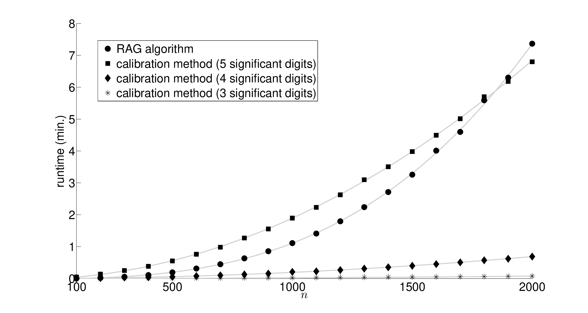
Figure 2 plots the measured cumulative runtimes versus the intermediate horizon or stage for the instance with states. Cumulative runtimes for the final stage are not included, since the RAG algorithm does not perform the bottleneck update at the last stage, and hence the latter’s cumulative runtime is about the same as that for the previous stage . The solid lines shown are polynomial LS fits for the predicted cumulative runtimes, of 2nd order for the RAG algorithm, and of 1st order (linear fit) for the calibration method, as predicted by the theoretical complexities. In the case of the RAG algorithm, the 2nd-order LS fit for the predicted cumulative runtime of a -state instance up to and including stage is . The RMSE is min., slightly under 1 sec., a very small value relative to the range of runtimes. To test the validity of the theoretical quadratic complexity on , the data were also fitted by a polynomial with one order less and of one order more than 2. While the linear LS fit is clearly inadequate, using a polynomial of order 3 gives the predicted cumulative runtime fit , with the RMSE dropping to min. Since the RMSE for the 2nd-order fit is already very small, and the leading coefficient of the 3rd-order fit is rather small, we conclude that the cumulative runtime performance is best fittedted by a 2nd-order polynomial, consistently with the theoretical complexity in . Still, despite its higher complexity, the RAG algorithm is faster than the calibration method with 5 significant digits up to and including a horizon of .
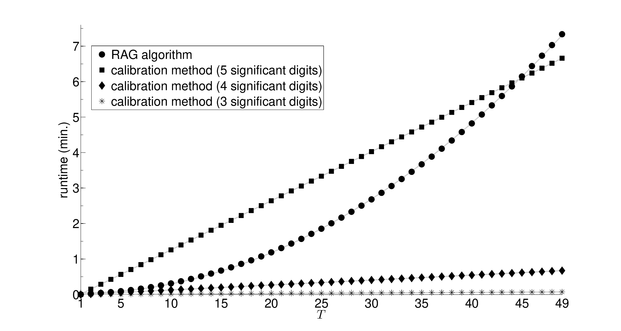
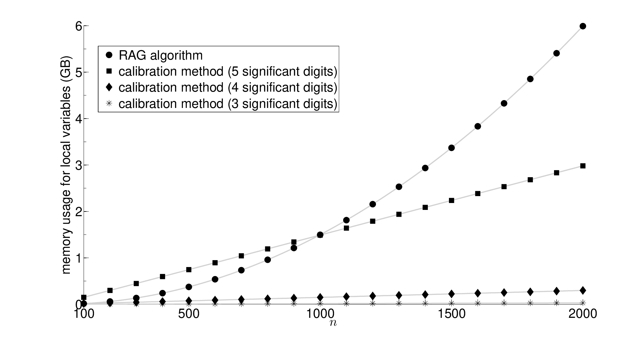
Figure 3 plots the required memory storage for floating-point local variables (in GB, excluding input and output, and using 8-byte double-precision numbers) versus for . In the author’s implementations, the RAG algorithm uses floating-point storage locations for local variables, whereas the calibration method with a grid of size uses locations. Note that, despite its higher complexity, the RAG algorithm uses less memory than the calibration method with 5 significant digits up to and including states. Note further that the local memory storage of the RAG algorithm grows linearly in the horizon , whereas that of the calibration method remains constant as varies.
6.2 Index computation for an infinite-state project
The next experiment aims to assess the actual runtime and memory
performance of the
index algorithm in Section 4
for a countably-infinite state project, for which the classic Bernoulli bandit
model with Beta priors is chosen, by benchmarking it against
the
calibration method. Recall from Section 4 that Theorem 4.3
establishes an
time complexity and an memory complexity
for such a version of the RAG algorithm, which in the case of a
Bernoulli bandit starting at with a horizon computes
relevant index values.
For fairness of comparison, the calibration method was modified to compute
approximately only such relevant index values.
To improve runtimes and exploit the reduced arithmetic and memory
operations due to sparsity of the transition probability matrix, the
author
developed
Fortran implementations that use threaded
routines from the Intel Math Kernel Library,
in particular the Sparse BLAS Level 3
MKL_DCOOMM subroutine
for sparse matrix multiplication.
Taking as the initial state, the algorithm in Section 4 was run on instances with horizons , computing all relevant index values in each case. As before, the calibration method (with to significant digits) was used for comparison.
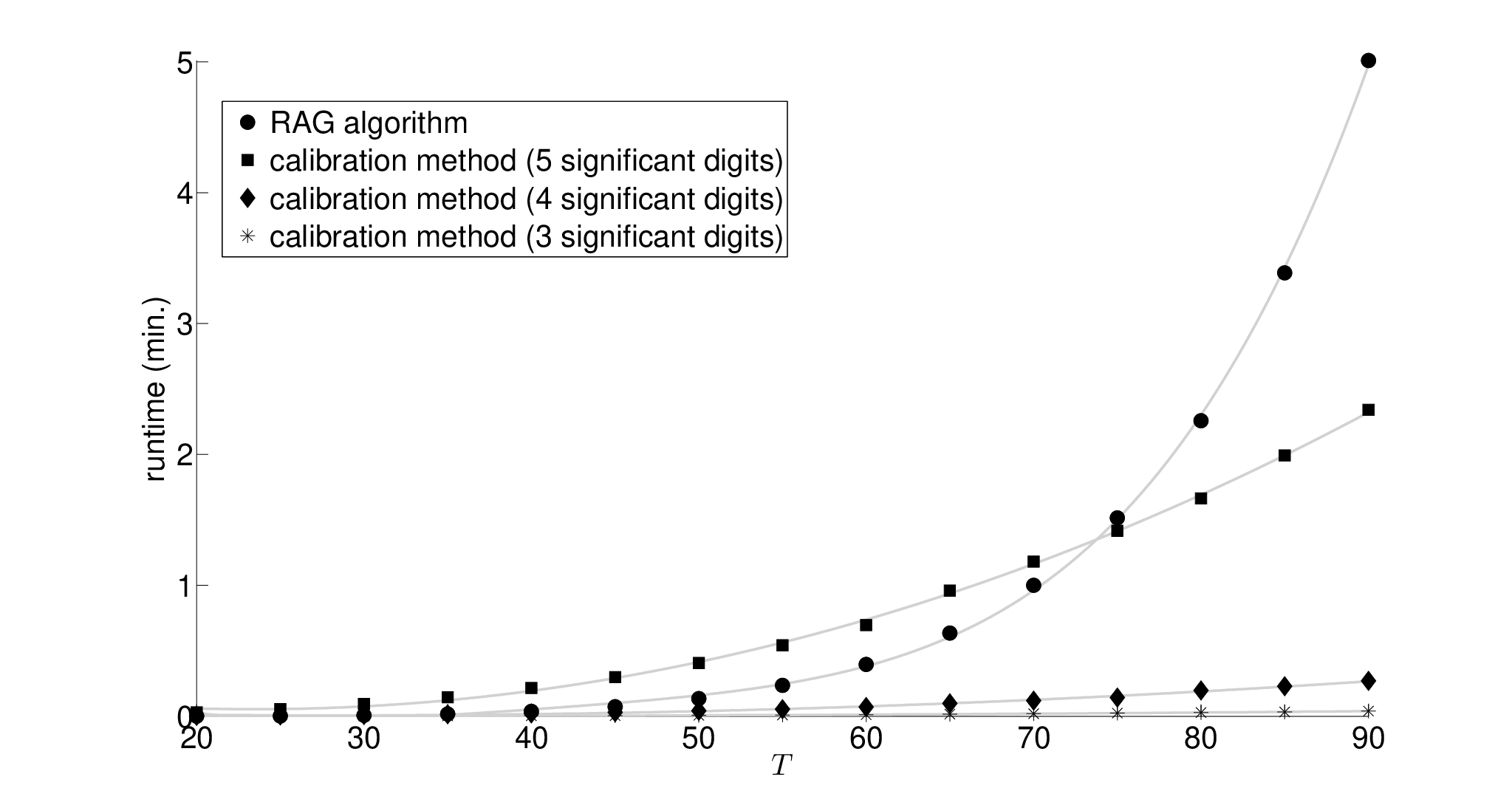
Figure 4 plots the measured runtimes versus the horizon . The solid lines shown were obtained by polynomial least-squares (LS) fit, of order for the algorithm, and of order for the calibration method. In the case of the algorithm, the 6th-order LS fit for the predicted runtime of an instance with remaining periods is . The RMSE is very small: min. To test the validity of the theoretical 6th-order complexity on , the data were also fitted by polynomials of orders 7, 5, 4, and 3. Using a 7th-order polynomial does not improve the RMSE. A 5th-order polynomial fit gives still a very small RMSE of min. (under 1 sec.), while a 4th-order polynomial fit has a small RMSE of min. (about 2 sec.), and a 3rd-order fit has a much larger RMSE of min. These results suggest that the predicted runtime of the algorithm is best fitted by a polynomial of lower order than the theoretical 6th-order complexity, with the 4th-order fit appearing to be best. As for the calibration method with significant digits, the 2nd- and 3rd-order fits have roughly equal RMSEs of about min., whereas the 1st-order fit has a large RMSE of min. Hence, the best fit for the predicted runtime of the calibration method is . Yet, note that the algorithm is faster than the calibration method with 5 significant digits up to and including horizon .
As for the actual memory usage of each algorithm (for local variables, excluding input and output), Figure 5 plots the required memory storage for floating-point local variables (excluding input and output, and using 8-byte double-precision numbers) versus . In the author’s implementations, the algorithm uses floating-point storage locations for local variables, whereas the calibration method with a grid of size uses storage locations. Note that, despite its higher complexity, the RAG algorithm uses less memory than the calibration method with 5 significant digits up to and including horizon .
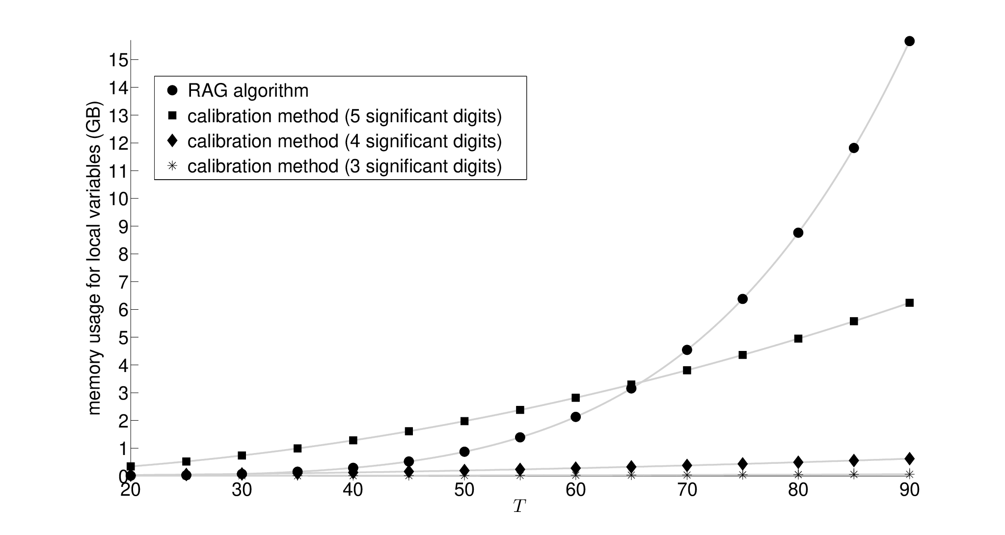
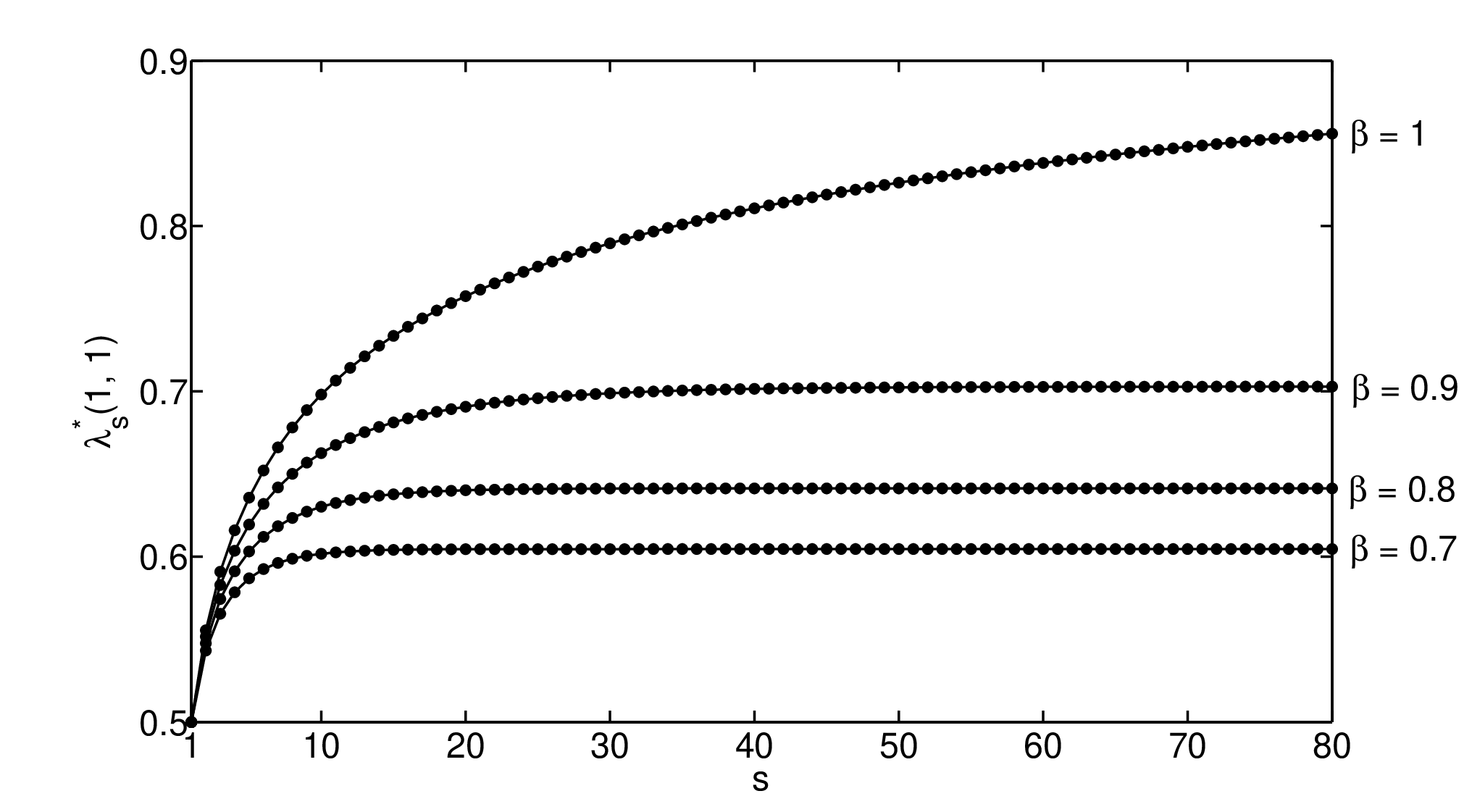
Figure 6 plots index versus the horizon , for discount factors . For each discount factor, the plotted index values were obtained from a single run of algorithm RAG with a horizon of .
7 Conclusions
This paper has introduced a recursive adaptive-greedy (RAG) algorithm for the efficient exact computation of a classic index for finite-horizon bandits, which performs only arithmetic operations. The algorithm has been compared with the standard calibration method, which computes approximate index values. When the latter method is used with a grid having the same size as the number of index values to be evaluated, both methods have the same time and memory complexities. Yet, for a fixed grid, the calibration method’s time and memory complexity are one order of magnitude lower than those of the RAG algorithm. Complementing such theoretical results, the computational study reported above shows that, if 3 or 4 significant digits of accuracy suffice, or if the number of states or the horizon are rather large, the calibration method is the best choice. Yet, the results also show that the RAG algorithm outperforms (with respect to both runtimes and memory) the calibration method with significant digits of accuracy in instances of moderately large size.
Acknowledgments
The author thanks the Associate Editor and an anonymous reviewer for constructive comments that helped improve the paper, including suggestions to compare the proposed algorithm with the calibration method, and to test the validity of the least-squares fits used in the computational experiments. This work was supported in part by the Spanish Ministry of Education and Science under project MTM2007-63140 and an I3 faculty endowment grant.
References
- Bellman (1956) Bellman, R. 1956. A problem in the sequential design of experiments. Sankhyā 16 221–229.
- Berry and Fristedt (1985) Berry, D. A., B. Fristedt. 1985. Bandit Problems: Sequential Allocation of Experiments. Chapman and Hall, London, UK.
- Bradt et al. (1956) Bradt, R. N., S. M. Johnson, S. Karlin. 1956. On sequential designs for maximizing the sum of observations. Ann. Math. Statist. 27 1060–1074.
- Caro and Gallien (2007) Caro, F., J. Gallien. 2007. Dynamic assortment with demand learning for seasonal consumer goods. Management Sci. 53 276–292.
- Dongarra and Eijkhout (2000) Dongarra, J. J., V. Eijkhout. 2000. Numerical linear algebra algorithms and software. J. Comput. Appl. Math. 123 489–514.
- Ginebra and Clayton (1999) Ginebra, J., M. K. Clayton. 1999. Small-sample performance of Bernoulli two-armed bandit Bayesian strategies. J. Statist. Planning Inf. 79 107–122.
- Gittins (1979) Gittins, J. C. 1979. Bandit processes and dynamic allocation indices. J. Roy. Statist. Soc. Ser. B 41 148–177.
- Gittins (1989) Gittins, J. C. 1989. Multi-armed Bandit Allocation Indices. Wiley, Chichester, UK.
- Gittins and Jones (1974) Gittins, J. C., D. M. Jones. 1974. A dynamic allocation index for the sequential design of experiments. J. Gani, K. Sarkadi, I. Vincze, eds., Progress in Statistics (European Meeting of Statisticians, Budapest, 1972). North-Holland, Amsterdam, The Netherlands, 241–266.
- Niño-Mora (2001) Niño-Mora, J. 2001. Restless bandits, partial conservation laws and indexability. Adv. Appl. Probab. 33 76–98.
- Niño-Mora (2002) Niño-Mora, J. 2002. Dynamic allocation indices for restless projects and queueing admission control: a polyhedral approach. Math. Program. 93 361–413.
- Niño-Mora (2005) Niño-Mora, J. 2005. A marginal productivity index policy for the finite-horizon multiarmed bandit problem. CDC-ECC ’05: Proc. 44th IEEE Conf. Decision and Control and European Control Conf. 2005 (Seville, Spain). IEEE, 1718–1722.
- Niño-Mora (2007) Niño-Mora, J. 2007. A fast-pivoting algorithm for the Gittins index and optimal stopping of a Markov chain. INFORMS J. Comput. 19 596–606.
- Niño-Mora (2008) Niño-Mora, J. 2008. Computing an index policy for multiarmed bandits with deadlines. ValueTools ’08: Proc. 3rd Int. Conf. Performance Evaluation Methodologies and Tools (Athens, Greece). ICST, Brussels, Belgium.
- Robbins (1952) Robbins, H. 1952. Some aspects of the sequential design of experiments. Bull. Amer. Math. Soc. 58 527–535.
- Varaiya et al. (1985) Varaiya, P. P., J. C. Walrand, C. Buyukkoc. 1985. Extensions of the multiarmed bandit problem: the discounted case. IEEE Trans. Automat. Control 30 426–439.
- Wang (1997) Wang, Y.-G. 1997. Error bounds for calculation of the Gittins indices. Austral. J. Statist. 39 225–233.