On a federated architecture for utilizing domain-specific descriptive modelsThanks: This work was carried out and funded in the framework of the Labex MS2T. It was supported by the French Government, through the program "Investments for the future" managed by the National Agency for Research (Reference ANR-11-IDEX-0004-02). This work was co-funded by the Airbus Defence and Space company. Affiliation: ^1,2

Defining the structure of models as a symmetric multicategory denoted Msc  is done in two stages. We start by defining a symmetric monoidal category (SMC) denoted (Mscm, $\otimes$, I) and prove that it is indeed an SMC. We then derive Msc  using results from [13]. Since we will be using matrices to define the composition in Mscm, we may be able to derive a further symmetric multicategory denoted MatMsc, where arrows are given by matrices that might be useful for computations.

Why is it not enough simply to derive an SMC? Consider the box $Y$ in Figure 2, composed of 2 boxes $X_{1}$ and $X_{2}$ . In an SMC $Y$ can be seen to be composed of $X_{1}\otimes X_{2}$ (i.e. there is an arrow $X_{1}\otimes X_{2}\to Y$), yielding Figure 2. Figure 2 is a lot clearer than Figure 2, in which the modularity (i.e. the clear distinction between $X_{1}$ and $X_{2}$ in $Y$) is not reflected graphically. Figure 2 corresponds to an arrow $X_{1},X_{2}\to Y$ in the multicategory. However, it is more convenient to use the SMC than the multicategory insofar as subscripts can be avoided.

The box and arrow representation that we use should not be confused with string diagrams [18]. String diagrams are a graphical language of categories [18] in which the objects and morphisms of categories are represented by wires and boxes respectively. In our paper, on the other hand, objects correspond to boxes, and morphisms correspond to how composite boxes are internally built (using wiring patterns) with its constituent boxes.

Figure 2 looks like a Wiring Diagram WD [20] [25], but in fact it differs from a WD in the following respects. In figure 2 we allow unconnected ports (ports without incoming or outgoing wires), converging wires (separate wires with the same target port), and diverging wires (same source port). Unconnected ports and converging wires are prohibited in a WD. Figure 2 would also allow several links between a source port and a target port. WDs may therefore be considered as special cases of figure 2 that include certain restrictions; this is discussed in Section 4.2. The point of allowing these various things is to encompass as many wiring patterns as possible that may occur in practice. For instance, it might be the case, structurally, that an actual component is not plugged into its surrounding environment via any of its interfaces. See for instance a simple Ptolemy model [24, Figure 9], similarly permissive.

$\bullet$ Objects $\textbf{Mscm}_{0}$. An object $a\in\textbf{Mscm}_{0}$ is a box and consists of a tuple $(in(a),out(a))$, where $in(a)$ and $out(a)$ are the finite sets of input (left) and output (right) ports of (the box) $a$ such that $in(a)\cap out(a)=\emptyset$. We additionally require that R1: the set of ports (i.e. $in(a)\cup out(a)$) be pairwise disjoint for all objects in $\textbf{Mscm}_{0}$.

$\bullet$ Arrows Mscm$(b;a)$. An arrow $b\xrightarrow{\theta}a$ indicates how a box $a$ is internally built from the box $b$. It consists of a tuple $(\theta^{in},\theta^{out})$

where $L^{in}$ and $L^{out}$ are the abstract finite sets of links coming respectively into an input port and an output port of one of the boxes $b$ and $a$.

We require that R2: $L^{in},L^{out}\in K$ and $L^{in}\cap L^{out}=\emptyset$. $(K,\cup,\cdot,\emptyset,\{\epsilon\})$ is a semiring introduced below to define composition using matrices and detailed in Appendix (Section 6). We additionally require that R3: the domains (or more precisely $L^{in}\cup L^{out}$) of the set of morphisms be pairwise disjoint. R1, R2 and R3 ensure that objects and morphisms are all unambiguously defined. This will also be important in the definition of the monoidal product. Note also that (1) does not allow a link to go from an output port of $a$ to one of its input ports. This is a modelling choice consistent with the fact that any box only exposes its input and output ports. An arrow is intended to give the internal wiring pattern of a composite box. A link that goes from an output port of $a$ to one of its input ports should, rather, give rise to a new object $a^{\prime}$ and a new arrow $a\to a^{\prime}$ which models a kind of self-feedback, see Figure 4.

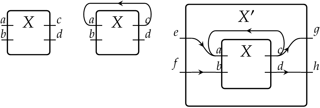
In the same way, (1) does not allow a link to go directly from an input port of $a$ to an output port. This is also a modelling choice that allows us to consistently zoom in on a composite box, avoiding the presence of isolated links when applying composition. If there were an isolated link, we would simply need to create a basic box with one input port and one output port and link them to the input and output ports respectively of $a$, such that this box outputs onto its output port the data that comes into its input port.

Example Consider Figure 3. We have two boxes X and Z given by $(\{a,b\},\{c,d\})$ and $(\{i,j\},\{k,l\})$ respectively. There is an arrow $X\to Z$ given by ({$l_{1}\mapsto(a,c),l_{2}\mapsto(b,i),l_{3}\mapsto(b,j)$},{$l_{4}\mapsto(k,c),l_{5}\mapsto(l,d)$}).

$\bullet$ Identities Mscm$(a;a)$. An identity $a\xrightarrow{1_{a}}a$ consists of $\theta^{in}$ and $\theta^{out}$ given by
$(1^{in}_{a},1^{out}_{a}):=(\{lin_{i}\mapsto(i,i),i\in in(a)\},\{lout_{j}\mapsto(j,j),j\in out(a)\})$ ; i.e. links connect identical (input to input and output to output respectively) ports from the domain ($a$) to the codomain ($a$) of $1_{a}$.

$\bullet$ Composition formula $\circ$. Composition enables a constituent of a composite box to be replaced by a more detailed constituent(s). For boxes $a,b,c\in$ Mscm₀, we have a function $\circ$:

$\textbf{Mscm}(b;a)\times\textbf{Mscm}(c;b)\rightarrow\textbf{Mscm}(c;a)$.

We must define an arrow $c\xrightarrow{\theta\circ\theta_{1}}a$. This amounts to finding a function $\theta_{0}:=\theta\circ\theta_{1}$, i.e. $\theta^{in}_{0}$ and $\theta^{out}_{0}$ following (1).

In order to define the composition formula, we use matrix operations. We start by establishing a connection between arrows and certain matrices over a semiring $(K,\cup,\cdot,\emptyset,\{\epsilon\})$; see Appendix 6 for more details. We are now ready to work with the matrix representation of an arrow.

The data (1) of an arrow can be rewritten as follows (see Appendix 6). We define

where $Y^{in}=in(b)$, $Y^{out}=out(b)$, $Z^{in}=in(a)$ and $Z^{out}=out(a)$. $2^{L}$ is the powerset.

Let $X^{in}=in(c)$, $X^{out}=out(c)$.

We denote $\emptyset_{M}$ as the matrix with $\emptyset$’s everywhere and $\mathbb{I}_{M}$ the square matrix with $\{\epsilon\}$’s on the main diagonal and $\emptyset$’s elsewhere.

Given (9) in Appendix 6 and the above notations, we are now ready to define arrow composition.

The map $\theta\circ\theta_{1}$ (i.e., $c\xrightarrow{\theta_{0}}a$ in Mscm) of an arrow is rewritten as $(O^{in},O^{out})$, given by the dashed arrows in the following diagrams. In accordance with Appendix 6 an arrow $I\xrightarrow{M}J$ in this diagram defines the matrix $M(I,J)$.
$\begin{array}[]{lr}\lx@xy@svg{\hbox{\raise 2.5pt\hbox{\kern 26.2274pt\hbox{\ignorespaces\ignorespaces\ignorespaces\hbox{\vtop{\halign{\entry@#!@&&\entry@@#!@\cr&\cr&\crcr}}}\ignorespaces{\hbox{\kern-11.67102pt\raise 0.0pt\hbox{\hbox{\kern 0.0pt\raise 0.0pt\hbox{\hbox{\kern 3.0pt\raise-2.5pt\hbox{$\textstyle{{X^{in}\ignorespaces\ignorespaces\ignorespaces\ignorespaces}\ignorespaces\ignorespaces\ignorespaces\ignorespaces}$}}}}}}}\ignorespaces\ignorespaces\ignorespaces\ignorespaces{}{\hbox{\lx@xy@droprule}}\ignorespaces\ignorespaces\ignorespaces{\hbox{\kern-20.65657pt\raise-14.74998pt\hbox{{}\hbox{\kern 0.0pt\raise 0.0pt\hbox{\hbox{\kern 3.0pt\hbox{\hbox{\kern 0.0pt\raise-1.89168pt\hbox{$\scriptstyle{N_{in}}$}}}\kern 3.0pt}}}}}}\ignorespaces{\hbox{\kern 0.0pt\raise-23.99998pt\hbox{\hbox{\kern 0.0pt\raise 0.0pt\hbox{\lx@xy@tip{1}\lx@xy@tip{-1}}}}}}{\hbox{\lx@xy@droprule}}{\hbox{\lx@xy@droprule}}\ignorespaces\ignorespaces\ignorespaces{}\ignorespaces\ignorespaces{\hbox{\lx@xy@drawline@}}\ignorespaces\ignorespaces\ignorespaces{\hbox{\kern 40.2926pt\raise 6.17508pt\hbox{{}\hbox{\kern 0.0pt\raise 0.0pt\hbox{\hbox{\kern 3.0pt\hbox{\hbox{\kern 0.0pt\raise-3.17508pt\hbox{$\scriptstyle{O^{in}}$}}}\kern 3.0pt}}}}}}\ignorespaces{\hbox{\kern 88.78378pt\raise 0.0pt\hbox{\hbox{\kern 0.0pt\raise 0.0pt\hbox{\lx@xy@tip{1}\lx@xy@tip{-1}}}}}}\ignorespaces\ignorespaces{\hbox{\lx@xy@drawline@}}\ignorespaces{\hbox{\lx@xy@drawline@}}{\hbox{\kern 88.78378pt\raise 0.0pt\hbox{\hbox{\kern 0.0pt\raise 0.0pt\hbox{\hbox{\kern 3.0pt\raise-2.5pt\hbox{$\textstyle{Z^{in}\cup X^{out}}$}}}}}}}{\hbox{\kern-26.2274pt\raise-32.76083pt\hbox{\hbox{\kern 0.0pt\raise 0.0pt\hbox{\hbox{\kern 3.0pt\raise-2.5pt\hbox{$\textstyle{{Y^{in}\cup X^{out}}\ignorespaces\ignorespaces\ignorespaces\ignorespaces}$}}}}}}}\ignorespaces\ignorespaces\ignorespaces\ignorespaces{}{\hbox{\lx@xy@droprule}}\ignorespaces\ignorespaces\ignorespaces{\hbox{\kern 38.15085pt\raise-38.9359pt\hbox{{}\hbox{\kern 0.0pt\raise 0.0pt\hbox{\hbox{\kern 3.0pt\hbox{\hbox{\kern 0.0pt\raise-3.17508pt\hbox{$\scriptstyle{M^{\prime in}}$}}}\kern 3.0pt}}}}}}\ignorespaces{\hbox{\kern 74.2274pt\raise-32.76083pt\hbox{\hbox{\kern 0.0pt\raise 0.0pt\hbox{\lx@xy@tip{1}\lx@xy@tip{-1}}}}}}{\hbox{\lx@xy@droprule}}{\hbox{\lx@xy@droprule}}{\hbox{\kern 74.2274pt\raise-32.76083pt\hbox{\hbox{\kern 0.0pt\raise 0.0pt\hbox{\hbox{\kern 3.0pt\raise-2.5pt\hbox{$\textstyle{{Z^{in}\cup Y^{out}\cup X^{out}}\ignorespaces\ignorespaces\ignorespaces\ignorespaces}$}}}}}}}\ignorespaces\ignorespaces\ignorespaces\ignorespaces{}{\hbox{\lx@xy@droprule}}\ignorespaces\ignorespaces\ignorespaces{\hbox{\kern 114.76813pt\raise-14.75pt\hbox{{}\hbox{\kern 0.0pt\raise 0.0pt\hbox{\hbox{\kern 3.0pt\hbox{\hbox{\kern 0.0pt\raise-3.0466pt\hbox{$\scriptstyle{N^{\prime out}}$}}}\kern 3.0pt}}}}}}\ignorespaces{\hbox{\kern 114.76813pt\raise-5.5pt\hbox{\hbox{\kern 0.0pt\raise 0.0pt\hbox{\lx@xy@tip{1}\lx@xy@tip{-1}}}}}}{\hbox{\lx@xy@droprule}}{\hbox{\lx@xy@droprule}}\ignorespaces}}}}&\lx@xy@svg{\hbox{\raise 2.5pt\hbox{\kern 13.11195pt\hbox{\ignorespaces\ignorespaces\ignorespaces\hbox{\vtop{\halign{\entry@#!@&&\entry@@#!@\cr&\cr\crcr}}}\ignorespaces{\hbox{\kern-12.8689pt\raise 0.0pt\hbox{\hbox{\kern 0.0pt\raise 0.0pt\hbox{\hbox{\kern 3.0pt\raise-2.5pt\hbox{$\textstyle{{Z^{out}}\ignorespaces\ignorespaces\ignorespaces\ignorespaces\ignorespaces\ignorespaces\ignorespaces\ignorespaces}$}}}}}}}\ignorespaces\ignorespaces\ignorespaces{}\ignorespaces\ignorespaces{\hbox{\lx@xy@drawline@}}\ignorespaces\ignorespaces\ignorespaces{\hbox{\kern 19.31023pt\raise 6.0466pt\hbox{{}\hbox{\kern 0.0pt\raise 0.0pt\hbox{\hbox{\kern 3.0pt\hbox{\hbox{\kern 0.0pt\raise-3.0466pt\hbox{$\scriptstyle{O^{out}}$}}}\kern 3.0pt}}}}}}\ignorespaces{\hbox{\kern 49.11195pt\raise 0.0pt\hbox{\hbox{\kern 0.0pt\raise 0.0pt\hbox{\lx@xy@tip{1}\lx@xy@tip{-1}}}}}}\ignorespaces\ignorespaces{\hbox{\lx@xy@drawline@}}\ignorespaces{\hbox{\lx@xy@drawline@}}\ignorespaces\ignorespaces\ignorespaces\ignorespaces{}{\hbox{\lx@xy@droprule}}\ignorespaces\ignorespaces\ignorespaces{\hbox{\kern 0.0pt\raise-14.75pt\hbox{{}\hbox{\kern 0.0pt\raise 0.0pt\hbox{\hbox{\kern 3.0pt\hbox{\hbox{\kern 0.0pt\raise-3.0466pt\hbox{$\scriptstyle{M^{out}}$}}}\kern 3.0pt}}}}}}\ignorespaces{\hbox{\kern 0.0pt\raise-24.0pt\hbox{\hbox{\kern 0.0pt\raise 0.0pt\hbox{\lx@xy@tip{1}\lx@xy@tip{-1}}}}}}{\hbox{\lx@xy@droprule}}{\hbox{\lx@xy@droprule}}{\hbox{\kern 49.11195pt\raise 0.0pt\hbox{\hbox{\kern 0.0pt\raise 0.0pt\hbox{\hbox{\kern 3.0pt\raise-2.5pt\hbox{$\textstyle{X^{out}}$}}}}}}}{\hbox{\kern-13.11195pt\raise-32.43448pt\hbox{\hbox{\kern 0.0pt\raise 0.0pt\hbox{\hbox{\kern 3.0pt\raise-2.5pt\hbox{$\textstyle{{Y^{out}}\ignorespaces\ignorespaces\ignorespaces\ignorespaces}$}}}}}}}\ignorespaces\ignorespaces\ignorespaces{}\ignorespaces\ignorespaces{\hbox{\lx@xy@drawline@}}\ignorespaces\ignorespaces\ignorespaces{\hbox{\kern 26.76009pt\raise-21.62701pt\hbox{{}\hbox{\kern 0.0pt\raise 0.0pt\hbox{\hbox{\kern 3.0pt\hbox{\hbox{\kern 0.0pt\raise-3.0466pt\hbox{$\scriptstyle{N^{out}}$}}}\kern 3.0pt}}}}}}\ignorespaces{\hbox{\kern 52.10458pt\raise-5.5pt\hbox{\hbox{\kern 0.0pt\raise 0.0pt\hbox{\lx@xy@tip{1}\lx@xy@tip{-1}}}}}}\ignorespaces\ignorespaces{\hbox{\lx@xy@drawline@}}\ignorespaces{\hbox{\lx@xy@drawline@}}\ignorespaces}}}}\end{array}$

where $N^{in}$, $N^{\prime out}$, $M^{\prime in}$ are respectively given by:

and $M^{out}$, $N^{out}$ are respectively given by:

Example Figure 5 is the representation of two arrows $X\xrightarrow{\theta_{1}}Y$ and $Y\xrightarrow{\theta}Z$. The arrow $X\xrightarrow{\theta\circ\theta_{1}}Z$ is given by the matrices $O^{in}$ and $O^{out}$ computed as follows. The matrices $M^{out}$, $N^{out}$, $N^{in}$, $N^{\prime out}$ and $M^{\prime in}$ are the following.

It is easy to check that $O^{out}=M^{out}\times N^{out}$ and $O^{in}=N^{in}\times M^{\prime in\times}N^{\prime out}$ are given by the following matrices:

The composition in this example enables us to zoom in on $Z$, in other words to know how $Z$ is built from $X$, itself a constituent box of $Y$. After the composition the link in Figure 5 (a representation of the two arrows $X\xrightarrow{\theta_{1}}Y$ and $Y\xrightarrow{\theta}Z$) from the port $h$ of Y to its port $f$, vanishes in Figure 3 (the arrow $X\xrightarrow{\theta\circ\theta_{1}}Z$) resulting from the composition. There are two reasons for this: the port $f$ is not connected in $X\xrightarrow{\theta_{1}}Y$, and the way $\cdot$ acts on links (or elements of $K$) in the semiring $(K,\cup,\cdot,\emptyset,\{\epsilon\})$. In practice this could mean that $f$ is not connected, even though it appears to be.

Note here that the effect of the tensor on different objects and arrows is simply to stack them straightforwardly and without losing (thanks to R1, R2 and R3) the origins of ports and links. For instance, stacking the unit I with any non-unit object $X$ will have no effect on $X$, since the box corresponding to I does not have any input or output ports. The effect of tensor on the same object (resp. arrow) is: stacking a box (resp. an arrow) with itself has no effect, i.e., results in the same object (resp. arrow).

Example In Figure 2, there is an arrow $X_{1},X_{2}\to Y$ in Msc, which is defined as $X_{1}\otimes X_{2}\to Y$ in (Mscm,$\otimes$).

Since we rely on matrix multiplication to define composition in Mscm, we can redefine the components of Msc using matrix without altering their initial meaning. This might be useful to automate computations with morphisms. Again a connection between morphisms of Mscm and certain matrices over a semiring is presented in Appendix 6.

The identity law holds in MatMsc with this rewriting (already shown in relation to Mscm) i.e. $m\circ 1_{X}=m=1_{Y}\circ m$ whenever $m:X\to Y$ is an arrow. The matrices defining $m\circ 1_{X}$ and $1_{Y}\circ m$ are both equal to $M$ i.e. $(M^{in},M^{out})$. The arrow $m\circ 1_{X}$ associates $M$ to $m$ and $N$ to $1_{X}$. Therefore $O^{in}$ equals $N^{in}\times M^{\prime in}\times N^{\prime out}=$

$O^{in}$ is indeed equal to $M^{in}$. We also have $O^{out}$ equals $M^{out}\times N^{out}=$

$O^{out}$ is equal to $M^{out}$. Hence, $m\circ 1_{X}=m$. In the same way: $m=1_{Y}\circ m$.

MatMsc can be seen as the category where objects declare interfaces and where morphisms declare how composite interfaces are internally built from other interfaces. The composition formula lets us safely zoom in and zoom out on levels further down and up in the hierarchy of interfaces.

It is worth noting that with only MatMsc (or Msc or Mscm), no meaning (related to a domain of interest or business domain) is assumed for an interface, its ports and, if applicable, its internal links.

The present section proposes an approach that seeks to bridge the gap between a possible semantics (interpretation of the structure) and its implementation in practice. A semantics corresponding to an interpretation of the structure may be formally defined in a variety of ways (denotational, axiomatic, operational, etc.) and with numerous possibilities of implementation. This paper is not concerned with defining or implementing a particular semantics, but sets out principles for formally connecting the structure, semantics and their implementation. As mentioned above, the architecture of a system is not about the effective (or final) implementation of the system.

Using the structure of models, it is possible to specify an interpretation of boxes such that the associated semantics can be recovered. An actual interpretation could therefore be independently developed by using the structure of models. Ideally, the specification of the interpretation is given by a functor $F:\textbf{Msc}\to\textbf{Msin}$, Msin being the category in which the structure is interpreted. The caveat ’ideally’ is necessary, because it may not always be straightforward to define a functorial semantics.

Examples

(i) Consider once again a model corresponding to the box shown in Figure 2. A domain-specific meaning of this model can only be known once the definition of an interpretation of its structure is given. Let us suppose that the domain of interest is classical physics and that we wish to study some physical properties of boxes. In this case, $F$ can be defined as $F:\textbf{Msc}\to\textbf{Msin}$. Let Msin :=Set. Along with objects, set of real numbers, and arrows, $n$-ary functions define the relationship between a physical property of a box and the physical properties of its $n$ constituent boxes. $F$ is a map of multicategories and an algebra for Msc (See [13, Definition 2.1.9, Definition 2.1.12]). Here, let us take mass to be the physical property under consideration.

Let $F$ be $F_{0}:\{X_{1},X_{2},Y\}\to\mathbb{R}_{>0}$ given by $X\mapsto ma$. The image of $X_{1},X_{2}\to Y$ is the function $F_{0}(X_{1})\times F_{0}(X_{2})\to F_{0}(Y)$ given by $(ma_{1},ma_{2})\mapsto ma$.

Depending on the meaning of links, $ma$ can be equal either to (*) $ma_{1}+ma_{2}$ or to (**) $ma_{1}+ma_{2}+m_{L}$, $m_{L}\in\mathbb{R}_{+}$ . In the first case (*), the mass of a composite box will depend solely on the masses of its constituent boxes. In the second case (**), the mass of a box will additionally depend on $m_{L}$, which is an additional mass emerging from internal connections.

Similar interpretations can be made for other physical properties.

(ii) Consider the arrow in Figure 6. Let each of the boxes $X_{i},i=1..4$ be interpreted as a two-digit adder ($d_{0}+d_{1}=cs$) which returns the sum ($s$) and the carry ($c$) via the top and bottom output ports respectively, given $d_{0}$ and $d_{1}$ obtained from top and bottom input ports. Here, the containing box $Y$ can be interpreted as two-digit numbers adder ($a_{1}a_{0}+b_{1}b_{0}=c_{2}c_{1}c_{0}$). There is a category (Msin) with five objects and one arrow.

The concept of mass in (i), and the concepts of two-digit adder and two-digit numbers adder in (ii), must be exposed by $F$, irrespective of how these concepts are defined in Msin and irrespective of the implementation. These data must be machine-accessible. It is worth noting that the functorial semantics of wiring diagrams (i.e. special cases of Msc) defined in [17], [20], [25] and [21] are concerned with the interconnections of discrete-time processes, databases and plug-and-play circuits, differential equations of open dynamical systems, and mode-dependent networks respectively. In each case, a particular algebra is devised which may be implemented as definitions of interpretations of the structure of models.

If the structure of a model is to be automatically exchangeable, then in the same way that the definition of an interpretation of the structure needs to be machine-accessible, the related data must also be machine-accessible.

The data relating to an actual (or candidate) system modelled is defined by a Set-valued functor $I:\textbf{Msc}\to\textbf{Set}$. This links an object $a\in\textbf{Msc}_{0}$ to the set of its usages $I_{0}(a)$, and any arrow $a_{1},...,a_{n}\xrightarrow{\theta}a\in C(a_{1},...,a_{n};a)$ to the function $I_{0}(a_{1})\times...\times I_{0}(a_{n})\xrightarrow{I(\theta)}I_{0}(a)$. Taking the composition and the identity in the same way as in Set, $I$ is a map of multicategories [13, Definition 2.1.9] and an algebra for Msc  [13, Definition 2.1.12]. The usefulness of $I$ stems from the fact that where the structure (Msc) of a model, together with at least one interpretation ($F$) of this structure, has been established, this is still not quite enough to allow the model to be used. The actual business data corresponding to the components of the structure are also required. For instance, consider the box shown in Figure 2 and the interpretation given in example (i) above. How do we communicate the fact that the masses of boxes $X_{1}$ and $X_{2}$ and $Y$ are given by actual values? No assumptions are made concerning the relations between the different masses. A parallel can be drawn with databases: it is good to have a database schema and to know what tables correspond to in the real world, but in order to use a database we also need to know the contents of the tables (the actual data entries). The purpose of $I$ is to answer this kind of question, by providing instances of the components of a structure of a model.

Let us recapitulate the purpose of the present section. We have provided an informal and a formal understanding of the proposed architecture FA. To be able to read a model (data), it is necessary to have at least the specification of $I:\textbf{Msc}\to\textbf{Set}$, while to be able to utilize a model (semantics), it is necessary to have at least the specification of $F:\textbf{Msc}\to\textbf{Msin}$.
$I$ and $F$ are intended to facilitate the transfer of the modularity of Msc  in different interpretations of Msc. Without functoriality, the modularity and the generality offered by the category-theoretic framework are lost (even though this functoriality is not always easily perceived, and may in some cases be unnecessary).

For exploiting models through a given automated routine, it is necessary to specify

and make the definition of interpretation machine-accessible. Nonetheless, wherever the usage of a structure is linked to a particular interpretation of that structure, it can be argued that the effective data related to Msc should instead be given by an amalgamated sum (a pushout) over (6).

FMI is a tool-independent interface that allows models to be exchanged and inter-operated in a co-simulation. An FMU (Functional Mock-up Unit), one of the components of FMI, must implement the FMI API via XML files and C-code. In FMI a model is associated with a particular FMU, which is generated using different tools. The kinds of models covered by FMI are (co) simulation models [2]. This paper is not primarily concerned with how models co-operate. Nevertheless, the way a model is defined (such as via an FMU) will influence how it can be reused.

An FMU separates the description of interface data (via an XML – Extensible Markup Language – file) from its mode of operation (via a program written in the C programming language). The interface data describes the static elements of the model such as type definitions (Real, Integer etc.), model variables, model structure (an ordered list of outputs termed Outputs, states termed Derivatives), and some initially unknown data termed InitialUnknowns), along with units etc.
The C-code and header files define the functions to be implemented by an FMU. These functions are used to simulate a model described according to a particular FMU. Generally speaking, the functions are for purposes such as initializing the FMU, assigning values to an input variable, retrieving the value of an output variable, changing the state of the FMU, etc. More information about the evolving specification of the FMI standard and supported tools can be found on the FMI website.

Although the FMI standard provides an interface to be implemented by FMUs, one concern is that there can be semantic gaps (studied in [22] [5]) between different model semantics (e.g, discrete events, dataflow models) or modelling languages and the target interface [23]. The semantics of the target interface has been considered as a timed Mealy machine [22]. Another concern is the extent to which the interface can be used to capture the semantics of different kinds of models [23]. Attempts to address this problem have resulted in various (proposed) adaptations of FMI [5] [4]. Therefore, the specification and definition of the common interface are crucial. The FMI standard is mainly concerned with the exchange of models and their simulation as black boxes.

In this paper we adhere to the FMI standard in separating structure and function. But, unlike in FMI, we give a formal definition of FA. The structures of models are considered as composite components defined within a category-theoretic framework, and a predefined interface for the implementation of functions is not imposed. Any implementation has to be derived from an interpretation of the structure of models. The (software) code corresponding to an implementation must expose the functions whose inputs and outputs are correlated to an interpretation of the structure. The data corresponding to the instantiations (i.e. actual serialized models) of the structure are elements that should be persisted as a file.

The kind of descriptive model that we are talking about is close, in terms of model structure (or abstract syntax), to the component-based, modular, and even composite-like models that are habitually encountered in system and software modelling, simulation, and more generally, analysis. See for instance [10] [24] for approaches and tools that deal with this kind of model structure. Although these approaches address modelling and simulation, their ultimate aim is not to solve the problem that is our concern here. They generally introduce their own approach (mainly on modelling formalisms) to system modelling and analysis. Metamodels for this kind of structure have been presented by [12] [10]. Their approaches advocate hierarchical and component-based design in systems modelling and engineering.

From a practical (yet formal) point of view, a box (a component of FA) is analogous to an actor in [24]. In [24], boxes are encoded using the logic of the modelling tool Ptolemy and the Java programming language. This may hamper the reuse of models, albeit some of these models may be imported using FMI.

In the present paper, unlike in [24], a box does not correspond to a particular semantics (i.e. the target of an interpretation of the structure). For [24], boxes or actors are seen as extended timed state machines, since the authors’ focus is on behavioural models. The corresponding semantics is also called the actor interface, defined in a way that includes both the structure and the semantics of the box. However, the actor interface can also be considered as the target of an interpretation of the structure of a box, since the input and output ports of a box are explicit in this interface. In [24] composite actors are basically considered as a set of actors, whereas for us a composite box is an arrow in Msc  (see Section 3). It will be noted that [24] is mainly concerned with a unified description of the behavioural semantics of a composite that comprises more than one actor.

It might be suggested that graphs are a way of formalizing the structure of models. Although graphs are very useful in representing interconnected objects, they lack the sort of intrinsic feature for dealing with the hierarchical composite structure of vertices (in the present context vertices equate to boxes) that we require. In order to represent this kind of structure, the graph would need to include additional data, which might complicate the formalization.

In fact, hierarchical graphs have also been formalized in category theory to model hierarchical structures [16] (where coupling of hyper-graphs and forests yields bigraphs) [3] (graphs inside graphs). Although hierarchical graphs encapsulate the hierarchy of nodes (here, boxes) and the communication links between nodes, the nature and structure of nodes and node containment (nesting) and links between nodes do not have the same meaning as described in Section 2. In the present work a node is given by input and output ports. The source and target of a link are ports at the same level of hierarchy of a box. We do not use two separate structures to define boxes (objects) and as a basis for composite boxes (arrows), and in this our approach contrasts with the two-structure approaches of [16] (place graph and linking graph ) and [3] (graph layer and hierarchical graph).

Our inspiration for the category structure considered in this paper is, rather, to be found in [20] [17], [25] and [14]. [14] considers symmetric monoidal and compact closed categories, with associated logics and proof theories as a possible formal foundation for systems engineering, given that it is compatible with current modelling languages and tools and encompasses existing formalisms. The mathematical object presented in this paper for encapsulating the structure of models, a symmetric multicategory (see Section 3), is closely related to the Wiring Diagrams (WD) structure developed in a series of papers: [17], [20], [25] etc. The two big differences between the WD structure and our structure are the following:

(i) Our structure is a more general construction supported by the "wiring" or connection pattern, i.e. almost all possible ways of connecting sub-components (or constituents) of a composite component are allowed, unlike WD (see Section 3.1 below for details of what WD does not allow). A WD is basically given by

which can be decomposed into two functions

To obtain (1) – our definition – from (8), the elements of $\phi^{in}$ and $\phi^{out}$ must be associated to the abstract sets of links or wires $L^{in}$ and $L^{out}$. To get (8) from (1) it is necessary to have $\theta^{in}$ and $\theta^{out}$ of (1) that are injective. The elements of $L^{in}$ and $L^{out}$ can be seen as the labels of wires.

(ii) We are not concerned with a particular interpretation (e.g. an algebra) of the structure of models.

The connection assumed in Definition 3.1 is established and proved in three steps as follows. (1) an equivalence between certain functions and matrices over a semiring is proved. Then (2) certain functions are shown to be equivalent to the morphisms of Mscm, by rewriting the signatures of morphisms’ component functions ($f^{in}$ and $f^{out}$). Finally, it is deduced (3) that a morphism of Mscm  yields a matrix being one of these certain matrices and the converse. Computations relating to morphisms are then made via matrices. Finally, matrix multiplication is used to obtain the composition formula of Mscm.

Let $K$ be the power set of the set of strings of finite lengths. $(K,\cup,\cdot,\emptyset,\{\epsilon\})$ is a semiring [7] where $\times:=\cdot$ is the product induced by the string concatenation operator, $+:=\cup$ is the addition given by union of sets of strings of finite lengths, $0:=\emptyset$ is the zero given by the empty set, and $1:=\{\epsilon\}$ is the unit given by the singleton set containing the empty string. Let also $I$ and $J$ be the finite sets with $n$ and $m$ elements respectively.

Henceforth, matrix multiplication is used for the composition formula of Mscm.

Example Let us consider $f_{A}:I_{1}\times S\to K$, and $f_{B}:S\times I_{2}\to K$ where $I_{1}=\{a,b\}$, $S=\{c,d\}$ and $I_{2}=\{e,f\}$.
Suppose given
$f_{A}:=\{(a,c)\mapsto\{w_{1}\},(a,d)\mapsto\emptyset,(b,c)\mapsto\{w_{2},w_{3}\},(b,d)\mapsto\emptyset\}$
$f_{B}:=\{(c,e)\mapsto\{w_{5}\},(c,f)\mapsto\emptyset,(d,e)\mapsto\emptyset,(d,f)\mapsto\emptyset\}$

The matrices $A$ and $B$ corresponding to the functions $f_{A}$ and $f_{B}$ are as follows.

The matrix $A$ means in practice that there is a link or wire ($w_{1}$) coming from the port $c$ and supplying the port $a$. There are also two links ($w_{2}$ and $w_{3}$) coming from $c$ and supplying $b$. The product $A\times B$ given by

shows in practice that there is also a link $(w_{1}w_{5}$) coming from $e$ and supplying $a$. Typically, a port will be either an input or output port of a box.

References

- [1]
- [2] Torsten Blochwitz, Martin Otter, Johan Akesson, Martin Arnold, Christoph Clauss, Hilding Elmqvist, Markus Friedrich, Andreas Junghanns, Jakob Mauss, Dietmar Neumerkel et al. (2012): Functional mockup interface 2.0: The standard for tool independent exchange of simulation models. In: Proceedings of the 9th International MODELICA Conference; September 3-5; 2012; Munich; Germany, 076, Linköping University Electronic Press, pp. 173–184.
- [3] Roberto Bruni, Andrea Corradini, Fabio Gadducci, Alberto Lluch-Lafuente & Ugo Montanari (2011): Hierarchical Models for Service-Oriented Systems. In: Rigorous Software Engineering for Service-Oriented Systems - Results of the SENSORIA Project on Software Engineering for Service-Oriented Computing, pp. 349–368, 10.1007/978-3-642-20401-2_16. Available at https://doi.org/10.1007/978-3-642-20401-2_16.
- [4] Fabio Cremona, Marten Lohstroh, David Broman, Edward A Lee, Michael Masin & Stavros Tripakis (2019): Hybrid co-simulation: it’s about time. Software & Systems Modeling 18(3), pp. 1655–1679.
- [5] Fabio Cremona, Marten Lohstroh, Stavros Tripakis, Christopher Brooks & Edward A Lee (2016): FIDE: an FMI integrated development environment. In: Proceedings of the 31st Annual ACM Symposium on Applied Computing, ACM, pp. 1759–1766.
- [6] Zinovy Diskin & Tom Maibaum (2014): Category theory and model-driven engineering: from formal semantics to design patterns and beyond. Model-Driven Engineering of Information Systems: Principles, Techniques, and Practice, p. 173.
- [7] Manfred Droste & Werner Kuich (2009): Semirings and Formal Power Series, pp. 3–28. Springer Berlin Heidelberg, Berlin, Heidelberg, 10.1007/978-3-642-01492-5_1.
- [8] Andrée C Ehresmann & J-P Vanbremeersch (1987): Hierarchical Evolutive Systems: A mathematical model for complex systems. Bulletin of Mathematical Biology 49(1), pp. 13–50.
- [9] Rik Eshuis (2009): Reconciling statechart semantics. Science of Computer Programming 74(3), pp. 65–99.
- [10] Cécile Hardebolle & Frédéric Boulanger (2008): ModHel’X: A component-oriented approach to multi-formalism modeling. In: Models in Software Engineering, Springer, pp. 247–258.
- [11] David Harel (1987): Statecharts: A visual formalism for complex systems. Science of computer programming 8(3), pp. 231–274.
- [12] Edward A Lee (2010): Disciplined heterogeneous modeling. In: Model Driven Engineering Languages and Systems, Springer, pp. 273–287.
- [13] Tom Leinster (2003): Higher Operads, Higher Categories. arXiv preprint math0305049.
- [14] Dominique Luzeaux (2015): A Formal Foundation of Systems Engineering. In: Complex Systems Design& Management, Springer, pp. 133–148.
- [15] Saunders Mac Lane (1998): Categories for the working mathematician. 2nd ed., 2nd ed edition. New York, NY: Springer.
- [16] Robin Milner (2008): Bigraphs and Their Algebra. Electr. Notes Theor. Comput. Sci. 209, pp. 5–19, 10.1016/j.entcs.2008.04.002. Available at https://doi.org/10.1016/j.entcs.2008.04.002.
- [17] Dylan Rupel & David I Spivak (2013): The operad of temporal wiring diagrams: formalizing a graphical language for discrete-time processes. arXiv preprint arXiv:1307.6894.
- [18] Peter Selinger (2010): A survey of graphical languages for monoidal categories. In: New structures for physics, Springer, pp. 289–355.
- [19] Sanjit A Seshia, Natasha Sharygina & Stavros Tripakis (2014): Modeling for verification. Handbook of Model Checking, EM Clarke, T. Henzinger, and H. Veith, Eds. Springer.
- [20] David I Spivak (2013): The operad of wiring diagrams: Formalizing a graphical language for databases, recursion, and plug-and-play circuits. arXiv preprint arXiv:1305.0297.
- [21] David I Spivak (2015): Nesting of dynamic systems and mode-dependent networks. arXiv preprint arXiv:1502.07380.
- [22] Stavros Tripakis (2015): Bridging the semantic gap between heterogeneous modeling formalisms and FMI. In: Embedded Computer Systems: Architectures, Modeling, and Simulation (SAMOS), 2015 International Conference on, IEEE, pp. 60–69.
- [23] Stavros Tripakis (2016): Compositionality in the Science of System Design. Proceedings of the IEEE 104(5), pp. 960–972.
- [24] Stavros Tripakis, Christos Stergiou, Chris Shaver & Edward A Lee (2013): A modular formal semantics for Ptolemy. Mathematical Structures in Computer Science 23(04), pp. 834–881.
- [25] Dmitry Vagner, David I Spivak & Eugene Lerman (2015): Algebras of open dynamical systems on the operad of wiring diagrams. Theory and Applications of Categories 30(51), pp. 1793–1822.
6 Appendix
Connection between morphisms of Mscm of and certain matrices over a semiring