Generalized Deep Thermalization for Free FermionsPreprint: APS/123-QED
Abstract
In non-interacting isolated quantum systems out of equilibrium, local subsystems typically relax to non-thermal stationary states. In the standard framework, information on the rest of the system is discarded, and such states are described by a Generalized Gibbs Ensemble (GGE), maximizing the entropy while respecting the constraints imposed by the local conservation laws. Here we show that the latter also completely characterize a recently introduced projected ensemble (PE), constructed by performing projective measurements on the rest of the system and recording the outcomes. By focusing on the time evolution of fermionic Gaussian states in a tight-binding chain, we put forward a random ensemble constructed out of the local conservation laws, which we call deep GGE (dGGE). For infinite-temperature initial states, we show that the dGGE coincides with a universal Haar random ensemble on the manifold of Gaussian states. For both infinite and finite temperatures, we use a Monte Carlo approach to test numerically the predictions of the dGGE against the PE. We study in particular the -moments of the state covariance matrix and the entanglement entropy, finding excellent agreement. Our work provides a first step towards a systematic characterization of projected ensembles beyond the case of chaotic systems and infinite temperatures.
I Introduction
The established paradigm for quantum thermalization in isolated quantum systems is extremely simple, and yet surprisingly effective. When a system is initialized in a short-range correlated state, it predicts, under a few typicality assumptions, that the late-time properties of local subsystems are described by a thermal Gibbs ensemble Cazalilla and Rigol 2010; Polkovnikov et al. 2011; D’Alessio et al. 2016. In this framework, usually understood in terms of the eigenstate thermalization hypothesis Deutsch 1991; Srednicki 1994; Rigol et al. 2008, one is interested in a local subsystem, while its complement plays the role of a thermal bath which is assumed not to be observed (i.e. measured).
Thermalization and its mechanisms have been probed to exquisite detail in a number of cold-atomic experiments Trotzky et al. 2012; Langen et al. 2013; Geiger et al. 2014; Langen et al. 2015; Neill et al. 2016; Clos et al. 2016; Kaufman et al. 2016. In fact, these works fully demonstrate the ability of current setups to keep track of both subsystems and their complement, having access to information on the “bath” which is discarded in the traditional setting. Motivated by this, two recent works Cotler et al. 2021; Choi et al. 2021 have put forward a new perspective, in which one is interested in the ensemble describing a subsystem when its complement, , is observed via projective measurements. This gives rise to an ensemble of pure states in , called projective ensemble (PE), which can be thought of as a particular unraveling of the subsystem density matrix.
Based on numerical and experimental evidence, Refs. Cotler et al. 2021; Choi et al. 2021 found that, for chaotic dynamics and infinite-temperature initial states, the PE approaches a Haar-random ensemble over the set of pure states in , forming a quantum state design Renes et al. 2004; Ambainis and Emerson 2007. From the fundamental standpoint, the appeal of this result lies in its universality, as it is claimed to be independent of any microscopic detail. Subsequent work substantiated these findings, with rigorous results provided in Refs. Ho and Choi 2022; Claeys and Lamacraft 2022; Ippoliti and Ho 2022a for classes of chaotic dual-unitary quantum circuits Bertini et al. 2019a; Bertini et al. 2019b; Piroli et al. 2020, while further connections between the onset of thermalization and quantum state designs were investigated in Refs. Wilming and Roth 2022; Ippoliti and Ho 2022b.

A natural question is how this picture is modified in the presence of conservation laws, including in particular integrable systems Korepin et al. 1997; Essler et al. 2005; Takahashi 2005, nowadays easily realized experimentally Malvania et al. 2021; Langen et al. 2015; Wang et al. 2022. In this case, local subsystems approach a stationary state described by a generalized Gibbs ensemble (GGE) Rigol et al. 2007, built out of all the quasi-local conserved operators (or charges) Ilievski et al. 2015; Ilievski et al. 2016a; Vidmar and Rigol 2016; Essler and Fagotti 2016; Ilievski et al. 2016b; Piroli et al. 2016a; Piroli et al. 2017; Ilievski et al. 2017; Pozsgay et al. 2017. GGEs are interesting as they differ qualitatively from thermal states, representing non-equilibrium phases with possibly exotic features De Nardis et al. 2014; Wouters et al. 2014; Pozsgay et al. 2014; Piroli et al. 2016b; Calabrese et al. 2016. Accordingly, one can ask how local conservation laws affect the PE.
In this work, we tackle this problem in the simplest case of non-interacting systems. Focusing on the time evolution of fermionic Gaussian states in a tight-binding model, we put forward a random ensemble constructed out of the conserved charges, which we call deep GGE (dGGE), and provide evidence of its validity based on Monte Carlo computations. For infinite-temperature initial states, we show that the dGGE coincides with a universal Haar random ensemble on the manifold of Gaussian states, while, for generic initial states, we introduce a generalized Haar ensemble to account for the finite expectation values of the charges.
The rest of this work is organized as follows. In Sec. II we introduce the model we study. We also briefly recall the standard GGE and the PE. In Sec. III we put forward our general conjecture for the deep GGE, while Sec. IV shows how the latter leads to a universal ensemble for infinite-temperature initial states. Finally, our conclusions are consigned to Sec. V, while several appendices provide details on the most technical parts of our work.
II The model
We consider a chain of spinless fermions, described by the Hamiltonian
| (1) |
where , are canonical operators satisfying . We initialize the system in a short-range correlated state and consider a bipartition into a region and its complement , “the bath”, containing and sites, respectively, cf. Fig. 1. In the limit , the subsystem reaches a stationary state at large time . Since the model is integrable, it is described by a GGE Essler and Fagotti 2016. Namely, for any observable supported on , we have , where
| (2) |
Here are Lagrange multipliers fixed by the initial state, are integral of motions, , while is a normalization constant. For the Hamiltonian (1), can be identified with the momentum occupation numbers Calabrese et al. 2011; Calabrese et al. 2012a; Calabrese et al. 2012b; Fagotti and Essler 2013 , with the Fourier transform of .
In the definition of the GGE, is traced out. Instead, the PE Cotler et al. 2021; Choi et al. 2021 is constructed by measuring and keeping track of the bath. Given a pure state on and (in our case, the evolved state ), we consider measuring at each of the sites in . We denote by the outcomes [], occurring with probability . After the measurement, is in a pure state , and the PE reads
| (3) |
Averages over this ensemble coincide with expectation values over , but the PE contains more information encoded in the higher statistical moments
| (4) |
Refs. Cotler et al. 2021; Choi et al. 2021, showed that the PE assumes a universal form for chaotic Hamiltonians without conserved quantities, coinciding with a uniform Haar measure over all pure states in . Our goal is to characterize it in the opposite case of an integrable Hamiltonian such as (1).
To simplify the problem, we consider an initial Gaussian state Bravyi 2004
| (5) |
where is the number of particles, is the vacuum, while is a unitary operator. Since the Hamiltonian (1) is quadratic, remains Gaussian at all times. In fact, the same is true for the measurement process Bravyi 2004, i.e. the projected state is also Gaussian.
This observation allows us to simplify the analysis of the PE. Since Gaussian states satisfy Wick’s theorem and is conserved, all states in the PE (3) are completely determined by the corresponding covariance matrix
| (6) |
with . Thus, higher moments of the PE are encoded in the ensemble , and the -fold averaged covariance matrices
| (7) |
This is a significant simplification, as the size of covariance matrices scales linearly in the system size.
More importantly, both and can be computed exploiting Gaussianity Bravyi 2004, allowing us to derive exact determinant formulae which can be evaluated efficiently for large system sizes, cf. Appendix A. Still, computation of the averages in (7) remains hard, as the number of terms grows exponentially in . To overcome this problem, we have set up a Metropolis Monte Carlo approach, which allows us to sample and estimate the averages in (7). This method, which takes as an input the covariance matrix of the evolved state, , turned out to be very efficient, providing reliable numerical data up to and a relative error of order with Monte Carlo steps. We provide details of the method in Appendix B.
III The deep GGE
Our goal is to construct a random ensemble, the dGGE, matching the predictions of the PE in the limit , (in this order). It is useful to imagine that the sites in are measured sequentially. Each measurement induces a random non-linear transformation of the covariance matrix restricted to . For large , it is natural to assume that this causes enough scrambling that only a minimal amount of information on the initial state is retained. Thus, it is crucial to identify those features which are preserved by the measurements. Beyond Gaussianity, we know that the dGGE should at least feature complete information on the conserved charges , encoded in the Lagrange multipliers , as it is clear considering the first moment of the PE ensemble [the GGE (2)]. Following this logic, we propose the representative-state approach. Considering a pure Gaussian state , whose conserved charges match those of the initial state , we may define the dGGE as the ensemble obtained by performing projective measurements on subsystem , i.e.
| (8) |
Here is the probability of obtaining when measuring , while is the post-measurement state. To see that correctly reproduces the first moment of the PE (3), we invoke the generalized ETH Caux and Essler 2013; Caux 2016; Essler and Fagotti 2016, stating for all supported on and .
To test the validity of Eq. (8) beyond the first moment, we perform explicit numerical computations. To be concrete, we consider the dimer initial state
| (9) |
which is Gaussian and corresponding to a non-trivial GGE for , with occupations numbers
| (10) |
For finite , the PE is sampled using the Monte Carlo approach previously discussed. To sample from the dGGE, we follow two approaches. The simplest choice for the pure state in Eq. (8) is the single-eigenstate ensemble: is chosen as a simultaneous eigenstate of all conserved quantities such that the eigenvalues match the expectation values in 11 1 This definition is inspired by the analysis of Refs. Cotler et al. 2021, where the equivalence between single-eigenstate ensembles and the PE was established at infinite temperatures. In practice, we take an eigenstate of , , where are drawn randomly according to the distribution function . A second possibility is to identify with a randomly generated correlation matrix , where is a diagonal matrix with ’s and ’s. The unitary matrix is drawn from the following distribution over the appropriate Haar measure, once global symmetries have been taken into account (see below for an example)
| (11) |
Here is the Fourier-transform operator mapping the quasimomentum space to the real one. We call this the generalized Haar ensemble: the diagonal matrix contains Lagrange multipliers enforcing the constraints [ should not to be confused with appearing in the GGE]. The normalization is the Harish-Chandra-Itzykson-Zuber integral Harish-Chandra 1957; Itzykson and Zuber 1980; McSwiggen 2018. Its form is non-trivial but several approximation tools Collins 2003; McSwiggen 2018; Bun et al. 2014 allow determining the functional relation between the and , as we discuss in Appendix C.
We sample both the single-eigenstate and the canonical Haar ensembles via the same Monte Carlo approach used for the PE, cf. Appendices B and C. For sufficiently large , we have verified that the two choices for give indistinguishable numerical results, so that in the following we only report data from the single-eigenstate ensemble.
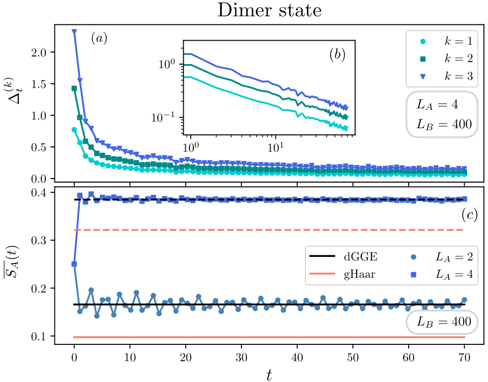
We computed the Frobenious norm Bhatia 2013 of the difference between the -fold averaged covariance matrices (7) in and , denoted by . An example of our data is reported in Fig. 2, convincingly showing convergence as . We see in particular a very clear power-law decay independently of .
As a second non-trivial test, we studied the average of the von Neumann entanglement entropy . Here, are two subsets of , with , while . Since is Gaussian, can be computed from Vidal et al. 2003, allowing us to sample it via Monte Carlo. Note that involves all higher moments of , yielding a non-trivial benchmark. In Fig. 2, we report our data for the space-averaged entanglement entropy , namely the sum of the values of the bipartite entanglement entropy at each point in , divided by . The plot shows very good agreement between the numerical simulation and the result of the ensemble (11). We stress that the entanglement entropy under consideration is not the one of the GGE, as this quantity is also not a linear functional of the density matrix. Overall, our results consistently support the equivalence between the dGGE and the PE. This is a non-trivial statement, implying that the mere knowledge of the conserved quantities is enough to reconstruct, not only the reduced density matrix, but also all higher moments in (4).
IV Infinite-temperature universal ensemble
The dGGE necessarily contains information on , strongly depending on . On the other hand, at infinite-temperatures the GGE loses any information on the latter, suggesting the possibility of a universal description of the PE. We show that this is the case. However, contrary to Refs. Cotler et al. 2021; Choi et al. 2021, the PE takes the form of a uniform measure over the manifold of fermionic Gaussian states. Closely related ensembles appeared in a number of recent works Liu et al. 2018; Zhang et al. 2020; Bianchi et al. 2021a; Bernard and Piroli 2021; Bianchi et al. 2021b; Murciano et al. 2022; Ulčakar and Vidmar 2022 and extend the notion of Haar-random states to non-interacting systems.
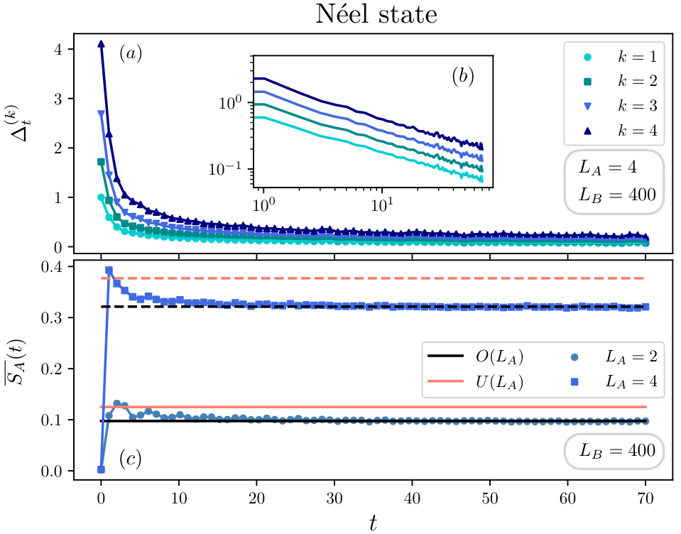
We focus on the “Néel” state, obtained by setting in (9), corresponding to an infinite-temperature state. From Eq. (10), one has , so that in Eq. (11). It follows that an appropriate correlation matrix for the whole system is obtained by drawing a unitary matrix from the Haar measure. In fact, additional constrains arise due to global symmetries. To elucidate this point, consider the change of basis . By inspection, we see that and the projected state are symmetric under time-reversal symmetry , i.e. their wave-function in the canonical basis defined by and is real. Therefore, the PE can only explore the sector of Gaussian states which is invariant under the joint global symmetry , and the corresponding ensemble in the space of covariance matrices can be defined as where is drawn from the uniform measure over the orthogonal group 22 2 Equivalently, one could choose to be drawn from the special orthogonal group . However, the two ensemble provide the same physical predictions.. Importantly, after the projective measurements, this ensemble can be reduced to one defined only on the sub-system . In particular, the invariance of the Haar measure under left/right multiplication is preserved by the projective measures for all orthogonal transformations restricted to . However, although has a well-defined particle number, this is not true for the subsystem , and after the measurement it collapses onto a pure state with particles, with some probability . One can see that the uniform measure with a fixed particle number for the whole system implies that this is only determined by an entropic factor, i.e. by the dimensions of the corresponding sector of the Hilbert space, and a random-matrix computation yields , cf. Appendix D. We thus arrive at the following prediction: the PE equals a grand canonical ensemble over different particle-number sectors each weighted with probability . In each sector, it takes the form
| (12) |
with uniformly distributed in . allows us to obtain explicit predictions, by either numerical sampling Mezzadri 2006 or analytic formulas derived using the properties of the Haar measure, cf. Appendix C. We have tested it against numerical sampling of the PE. As before, we have studied and the space-averaged entanglement entropy . An example of our data is reported in Fig. 3, displaying excellent agreement.
Our results show that the infinite-temperature PE is universal even for non-interacting systems, as it only depends on the Gaussianity of the model and on its global symmetries, but not on the details of the Hamiltonian. The same kind of universality was found for instance in Refs. Vidmar et al. 2017; Vidmar et al. 2018; Hackl et al. 2019; Lydzba et al. 2020; Lydzba et al. 2021, studying the averaged entanglement entropy of the eigenstates of quadratic Hamiltonians.
V Conclusions
We have studied the PE emerging at late times after quantum quenches in non-interacting integrable systems. We have characterized it in terms of a random ensemble, the dGGE, constructed out of the initial expectation value of the conserved charges. We have tested our predictions against Monte Carlo sampling of the PE, finding convincing agreement. From the fundamental point of view, our work reveals that, even in non-interacting systems, the PE is largely independent from microscopic details. In particular, at infinite-temperature it coincides with a universal Haar-random ensemble over the set of Gaussian states directly formulated in the subsystem Liu et al. 2018; Zhang et al. 2020; Bianchi et al. 2021a; Bernard and Piroli 2021; Bianchi et al. 2021b; Murciano et al. 2022. This fact could be useful for realizing related ensembles in practice, leveraging the intrinsic randomness of measurements and extending the logic of quantum state designs Choi et al. 2021; Cotler et al. 2021. For finite temperatures, the existence of a finite correlation length prevents the definition of a post-measurement ensemble expressed uniquely in terms of the charges of . However, this could be possible for . We leave this question for future work. Finally, it would be interesting to generalize our study for interacting integrable models where an extensive number of conserved quantities is still present but the Gaussian structure of correlations is lost.
Acknowledgements
J.D.N. acknowledges inspiring discussions with Wen Wei Ho. Some of his work was performed at Aspen Center for Physics, which is supported by National Science Foundation grant PHY-1607611 and at Galileo Galilei Institute during the scientific program “Randomness, Integrability, and Universality”. This work has been partially funded by the ERC Starting Grant 101042293 (HEPIQ). ADL acknowledges support by the ANR JCJC grant ANR-21-CE47-0003 (TamEnt).
Appendix A Covariance matrix after projective measurement of local densities
In this section we derive the transformation induced on the covariance matrix, defined for any pure state as
| (13) |
We will first consider the effect of measuring the density operator on a given site and subsequently the simultaneous effect of many single-site measurements altogether.
A.1 Single-site measurement
We foremost observe that after measuring the density operator , two outcomes are possible corresponding to the eigenvalue (empty site) or (occupied site). Denoting as the projector onto the corresponding eigenspace, the post-measurement state can be represented as
| (14) |
Upon an inessential normalisation, we can always represent the projector , i.e. the exponential of a quadratic operator. This implies that the projective measurement of a local density preserves the Gaussianity of the state. We can thus focus on the transformation induced on the covariance matrix . We have
| (15) |
where denotes the probability of obtaining the outcome after the measurement. Since after the measurement the state of site factorises, one must have
| (16) |
We can thus focus on the relevant submatrix with both . Let us focus for simplicity on the case . Then, Eq. (15) reduces to (see also e.g. Coppola et al. 2022)
| (17a) | |||
| for and | |||
| (17b) | |||
where the last equality follows from a simple application of Wick’s theorem. The other case can be obtained by a similar calculation or making use of the particle-hole symmetry and leads to
| (18a) | ||||
| (18b) | ||||
We can put together (17, 18) in the single equation
| (19a) | ||||
| (19b) | ||||
A.2 Measurements on multiple sites
Now that we understood the effect of measurement on one site, we can generalize it to multiple site measurements. Following the notation of the main text, we assume that the sites undergoing projective measurements of their local densities are all in the spatial region and we denote as , the outcomes of the measurements. We are interested in computing the resulting covariance matrix for and the joint probability of all outcomes .
A.2.1 Iterative procedure
Since the operators for all commute to one another, it is clear that measuring all sites in can be performed as a sequence of single-site measurements with outcomes , irrespectively of the order. In order to simplify the notation, we assume that the sites are measured from left to right and that the sites in are the leftmost ones. Let us denote as , i.e. the measurement outcomes of the leftmost sites in . Then, by making use of (19), we have
| (20a) | ||||
| (20b) | ||||
| (20c) | ||||
and the procedure finishes when as .
A.2.2 Determinant form
It is possible to derive a closed determinant form which expresses directly and . In order to do so, we introduce the matrix and the dimensional vectors as
| (21) |
also we denote as the restriction of to the sites in . Then, we can set
| (22) |
with the associated probability
| (23) |
The equivalence between the two procedures can be verified by induction.
As a benchmark, we check that the sum over all probabilities for all possible strings gives 1. Using the variables we have
| (24) |
We can expand the determinant as
| (25) |
Summing over we easily notice that only the first term contribute (since the other they miss at least one of the factors ), and the only term not giving zero is .
In practice, for numerical stability and efficiency, we found it more efficient to perform the measurements over the whole region using the iterative procedure (20).

Appendix B Montecarlo sampling of the Projected ensemble
In order to compute the PE at any time , we time evolve the correlations matrix using the single particle Hamiltonian
| (26) |
with the evaluated on the initial state, and at each time step we sample the PE by Monte Carlo procedure, namely given the correlation matrix at time , we start from a random sequence of zeros and 1, and we compute and using the iterative procedure (20). The next Monte Carlo step is to generate a new configuration by flipping one 0 or 1 at random within the sequence and to compute their ratio of corresponding probabilities
| (27) |
which is to be compared with a randomly generated real number in the interval . If the latter is smaller than the move is accepted and the new correlation matrix is computed as , otherwise is rejected and the sequence and the correlation matrix are left unchanged. The algorithm is then iterated on steps where all higher moments of the PE are taken as
| (28) |
In Fig. 4 we show the convergence of the von Neumann entropy at different times, by plotting the standard deviation sampled with 40 different realisations of , computed as
| (29) |
where is the entanglement entropy in the subsystem summed over all sites. The average values are the data reported in the main text. The plot shows that expected errors on the Monte Carlo averaging at late times are of order .
We note that for the measurements over a set of commuting quantities as we consider here, one can introduce a slightly simpler procedure, which avoids any correlation between configurations produced by the Montecarlo algorithm. In practice, in exactly steps, one generates an entire random sequence with the correct probability: the sites are sequentially measured from left to right, but choosing at each step
| (30) |
where the correlation matrix is obtained after the measurement of all sites up to (as explained in A.2.1). See for instance Coppola et al. 2022. Here, we choose to use the more general Montecarlo algorithm explained above.
Appendix C Generalised Haar ensemble
As discussed in the main text, a simple way to generate representative states is to sample randomly from an appropriate distribution over the Haar measure, thus enforcing the correct average expectation of the conserved charges. This could be constructed as follows. Because of the conservation of the number of particles, we can always assume that . However, we want to enforce the constraint about the occupation number in the Fourier basis , where performs the change of basis between the momentum and the real space basis. This naturally leads to the microcanonical Haar ensemble of covariance matrices
| (31) |
where is the normalization such that . Note that for an infinite temperature ensemble, for any , the delta functions impose no constraints at large and the matrices are simply drawn from the uniform distribution over the Haar measure. On the contrary, for generic the deltas forces a bias on the distribution of the matrix . For practical purposes, instead of working with (31), it is better to replace the delta constraint with the canonical Haar ensemble, defined by
| (32) | ||||
| (33) |
where we made use of the invariance of the Haar measure and introduce the diagonal matrix containing the Lagrange multipliers. Their value can be fixed via
| (34) |
We observe that for any constant . So, the solution of (34) are always defined up to a constant, which we fix by imposing the constraint
| (35) |
C.1 Gaussian approximation
A simple approximation for the integration over the Haar measure is obtained assuming that all entries of the matrix are Gaussian distributed for large . In the case of Eq. (33), for non-zero ’s, there is a competition between the constraint imposed by unitarity
| (36) |
and the one coming from Eq. (34). To enforce both constraints and a Gaussian distribution of the matrix entries, we rather consider the measure
| (37) |
and fix the Lagrange multiplier ’s and ’s via the conditions
| (38) | ||||
| (39) |
In the case of the unitary group, , the entries are Gaussian complex numbers, so that the integration measure factorises as
| (40) |
leading to the solutions
| (41) |
In the infinite temperature case, the filling function , all the biases consistently with the fact that one can simply sample from the pure Haar distribution.
In principle, one may wonder whether the additional constraint about the normalization of columns should also be imposed, i.e.
| (42) |
It is easy to verify that this constraint is automatically satisfied by the solution above, since
| (43) | ||||
| (44) |
where indicates the average with the measure in Eq. (37).
A similar approximation can be obtained for other groups, i.e. the orthogonal group, by appropriately changing the integration measure Eq. (40). The values of ’s given in Eq. (41) provide a good approximation when does not vary too much with , i.e. close to infinite temperature, but they are not exact in general. In the next sections, we show different methods to obtain more accurate evaluations.
C.2 Finite-size evaluation
The partition sum can actually be computed explicitly using the Harish-Chandran-Itzykson-Zuber Harish-Chandra 1957; Itzykson and Zuber 1980 formula. We recall that this formula gives the following integral
| (45) |
where is the spectrum of and we defined the Vandermonde determinant of a set as
| (46) |
Thus, if we define the diagonal matrix , the integral in (33) can be evaluated replacing and . However, the matrix has (several) degenerate eigenvalues, since its made of ones and zeros. In this case, a limit is required to properly compute the rhs of (45). To regularise, we set
| (47) |
and take the limit at the end. We have clearly
| (48) |
where is the Barnes G function. Ignoring numerical factors which are irrelevant in the normalisation, one has in the limit
| (49) |
where the matrix takes the form
| (50) |
Although exact, Eq. (49) does not allow an efficient evaluation at large , because as already seen in Eq. (41), the ’s become large with , thus making the exponentials in Eq. (50) hard to evaluate numerically.
C.3 High-temperature expansion
The large asymptotics of the HCIZ integral has been investigated in several papers Collins 2003; Bun et al. 2014, see also the introductory review McSwiggen 2018. One important result is that it is possible to write down explicitly the “large temperature” expansion of Eq. (33) directly in the limit of large in terms of combinatorial quantities. First of all, we know already from Eq. (41) that at large , the ’s are going to be scaled linearly with . So we set
| (51) |
where is the quasiparticle momentum in the thermodynamic limit. With this definition, we can express the moments of the matrix as
| (52) |
We can now introduce a free energy in the form
| (53) |
which is now a functional of . We have the expansion in powers of (see Eq.(2.10) in McSwiggen 2018)
| (54) |
where the sum runs over the partitions of the integer and are the monotonous Hurwitz numbers associated to the pair of partitions computed at genus Goulden et al. 2013 and we refer to McSwiggen 2018 for their combinatorial definition. The constraint Eq. (35) turns into the the equation
| (55) |
Expanding up to the third order (), one has
| (56) |
Taking the functional derivative and constraining (consistent with (35))
| (57) |
where is the particle density. One can easily verify that this is solved up to the order by
| (58) |
where the constant is put to enforce the constraint . The result is consistent with the Gaussian approximation in (41).
However, at the next order, deviations from the Gaussian approximation appear. As an example, we compute them for the case of the dimer states introduced in Eq. (9). Writing for generic , with and , we can write it explicitly as
| (59) |
After some manipulations, one obtains
| (60) |
which differs from the small expansion of the Gaussian approximation (41)
| (61) |
C.4 Montecarlo sampling from the generalised Haar ensemble
We now suppose that the values of the are known, and we want to sample from the distribution in Eq. (32). The problem has been also analysed in Leake et al. 2021, here we discuss a straightforward implementation based on the Metropolis–Hastings algorithm. To do so, we introduce a random walk in the group. We consider the Markov process at discrete time step
| (62) |
Let us first analyse the simple case , where one simply needs to sample in from the Haar distribution. Given a certain distribution measure over hermitian matrices (that we specify later on), one can set
| (63) |
We stress that the function refers to integration via the Haar measure, i.e., it is defined by
| (64) |
It is easy to verify from this definition that . Indeed,
| (65) |
where in the first equality we changed variable and we used the invariance of the Haar measure over left multiplication (). We thus see that if we choose , one immediately has
| (66) |
Thus, detail balance is fulfilled with the flat measure .
From this construction, it becomes clear how to modify the algorithm to obtain sampling from (32) via the usual Metropolis-Hastings formula. It is enough to set
| (67) |
In order to do so, it is convenient to specify further the distribution over the hermitian matrices . We choose it as rotations. In other words,
- •
we randomly choose a pair of distinct indices uniformly;
- •
we choose a direction with equal probabilities
- •
we choose a random “angle”
- •
we set
(68) where indicates a Pauli matrix in the subspace and the identity elsewhere.
- •
accept the new unitary
- –
with probability if both or , because in both these cases as the matrix restricted to is a multiple of the identity;
- –
with probability if , because and , as the transformation only adds a phase;
- –
with probability if but . Note that can be restricted to the subspace of indices .
- –
C.5 Self-improving Montecarlo method
The algorithm presented in the previous section assumes that the are given and allows sampling from Eq. (33). In reality, what is given is the density and the parameters are to be fixed from (34). In practice, starting from some initial estimation for the ’s, we can iteratively apply the MC procedure to gradually improve such an estimation. We introduce the functional
| (69) |
The optimal choice of the ’s lies at the minimum of . We can use gradient descent to improve the current estimation of :
| (70) |
where we used as a shortcut for . In practice, we run a few MC steps at fixed ’s, which allow estimating and . Then one can use (C.5) to update the values of the ’s. Note however that the fluctuations due to finite prevents from converging to arbitrary accuracy. In practice, after a few iterations, the algorithm cannot improve unless is increased.
Appendix D Number distribution in Gaussian states
In this section we prove the formula given in the main text about the distribution of the number of particles in the region . We assume that the whole system is in a random Gaussian state described by the ensemble of covariance matrices
| (71) |
where the parameter indicates: i) the orthogonal group (, ii) the unitary group . We set
| (72) |
where and the average is taken over the ensemble (71). We claim that the following formula holds
| (73) |
which has a simple combinatorial interpretation as splitting the particles such that are in and are in . Eq. (73) can be easily proven for random states over the whole Hilbert space Bianchi and Donà 2019; Murciano et al. 2022. In the Gaussian case, its proof is less evident.
We proceed as follows. We first of all introduce the generating function
| (74) |
where in the last equality we used Wick’s theorem to express the expectation value in terms of a determinant of the reduced covariance matrix to the region , i.e. for . From this construction, the matrix is known to be drawn from the Jacobi ensemble Forrester 2010. The joint probability distribution function of its eigenvalues takes the form
| (75) |
where the constants and . Setting , we can thus express
| (76) |
where in the last equality we used the symmetry of the integral under the permutation of the eigenvalues. The coefficients can be expressed in terms of the Aomoto’s integral Wikipedia contributors 2019; Aomoto 1987 and reads
| (77) |
Plugging this last expression in Eq. (76), we obtain the final formula
| (78) |
Now, standard manipulations of hypergeometric functions can be used to show that Eqs. (78,D) lead to Eq. (73), as expected.
References
- Cazalilla and Rigol (2010) M. Cazalilla and M. Rigol, New J. Phys. 12, 055006 (2010).
- Polkovnikov et al. (2011) A. Polkovnikov, K. Sengupta, A. Silva, and M. Vengalattore, Rev. Mod. Phys. 83, 863 (2011).
- D’Alessio et al. (2016) L. D’Alessio, Y. Kafri, A. Polkovnikov, and M. Rigol, Adv. Phys. 65, 239 (2016).
- Deutsch (1991) J. M. Deutsch, Phys. Rev. A 43, 2046 (1991).
- Srednicki (1994) M. Srednicki, Phys. Rev. E 50, 888 (1994).
- Rigol et al. (2008) M. Rigol, V. Dunjko, and M. Olshanii, Nature 452, 854 (2008).
- Trotzky et al. (2012) S. Trotzky, Y.-A. Chen, A. Flesch, I. P. McCulloch, U. Schollwöck, J. Eisert, and I. Bloch, Nature Phys. 8, 325 (2012).
- Langen et al. (2013) T. Langen, R. Geiger, M. Kuhnert, B. Rauer, and J. Schmiedmayer, Nature Physics 9, 640 (2013).
- Geiger et al. (2014) R. Geiger, T. Langen, I. Mazets, and J. Schmiedmayer, New J. Phys. 16, 053034 (2014).
- Langen et al. (2015) T. Langen, S. Erne, R. Geiger, B. Rauer, T. Schweigler, M. Kuhnert, W. Rohringer, I. E. Mazets, T. Gasenzer, and J. Schmiedmayer, Science 348, 207 (2015).
- Neill et al. (2016) C. Neill, P. Roushan, M. Fang, Y. Chen, M. Kolodrubetz, Z. Chen, A. Megrant, R. Barends, B. Campbell, B. Chiaro, et al., Nature Phys. 12, 1037 (2016).
- Clos et al. (2016) G. Clos, D. Porras, U. Warring, and T. Schaetz, Phys. Rev. Lett. 117, 170401 (2016).
- Kaufman et al. (2016) A. M. Kaufman, M. E. Tai, A. Lukin, M. Rispoli, R. Schittko, P. M. Preiss, and M. Greiner, Science 353, 794 (2016).
- Cotler et al. (2021) J. S. Cotler, D. K. Mark, H.-Y. Huang, F. Hernandez, J. Choi, A. L. Shaw, M. Endres, and S. Choi, arXiv:2103.03536 (2021).
- Choi et al. (2021) J. Choi, A. L. Shaw, I. S. Madjarov, X. Xie, J. P. Covey, J. S. Cotler, D. K. Mark, H.-Y. Huang, A. Kale, H. Pichler, et al., arXiv:2103.03535 (2021).
- Renes et al. (2004) J. M. Renes, R. Blume-Kohout, A. J. Scott, and C. M. Caves, J. Math. Phys. 45, 2171 (2004).
- Ambainis and Emerson (2007) A. Ambainis and J. Emerson, in Twenty-Second Annual IEEE Conference on Computational Complexity (CCC’07) (IEEE, 2007) pp. 129–140.
- Ho and Choi (2022) W. W. Ho and S. Choi, Phys. Rev. Lett. 128, 060601 (2022).
- Claeys and Lamacraft (2022) P. W. Claeys and A. Lamacraft, Quantum 6, 738 (2022).
- Ippoliti and Ho (2022a) M. Ippoliti and W. W. Ho, arXiv:2204.13657 (2022a).
- Bertini et al. (2019a) B. Bertini, P. Kos, and T. Prosen, Phys. Rev. X 9, 021033 (2019a).
- Bertini et al. (2019b) B. Bertini, P. Kos, and T. Prosen, Phys. Rev. Lett. 123, 210601 (2019b).
- Piroli et al. (2020) L. Piroli, B. Bertini, J. I. Cirac, and T. Prosen, Phys. Rev. B 101, 094304 (2020).
- Wilming and Roth (2022) H. Wilming and I. Roth, arXiv:2202.01669 (2022).
- Ippoliti and Ho (2022b) M. Ippoliti and W. W. Ho, Quantum 6, 886 (2022b).
- Korepin et al. (1997) V. E. Korepin, N. M. Bogoliubov, and A. G. Izergin, Quantum inverse scattering method and correlation functions, Vol. 3 (Cambridge university press, 1997).
- Essler et al. (2005) F. H. Essler, H. Frahm, F. Göhmann, A. Klümper, and V. E. Korepin, The one-dimensional Hubbard model (Cambridge University Press, 2005).
- Takahashi (2005) M. Takahashi, Thermodynamics of One-Dimensional Solvable Models (2005).
- Malvania et al. (2021) N. Malvania, Y. Zhang, Y. Le, J. Dubail, M. Rigol, and D. S. Weiss, Science 373, 1129 (2021).
- Wang et al. (2022) Q.-Q. Wang, S.-J. Tao, W.-W. Pan, Z. Chen, G. Chen, K. Sun, J.-S. Xu, X.-Y. Xu, Y.-J. Han, C.-F. Li, and G.-C. Guo, Light: Science & Applications 11 (2022), 10.1038/s41377-022-00887-5.
- Rigol et al. (2007) M. Rigol, V. Dunjko, V. Yurovsky, and M. Olshanii, Phys. Rev. Lett. 98, 050405 (2007).
- Ilievski et al. (2015) E. Ilievski, J. De Nardis, B. Wouters, J.-S. Caux, F. H. L. Essler, and T. Prosen, Phys. Rev. Lett. 115, 157201 (2015).
- Ilievski et al. (2016a) E. Ilievski, E. Quinn, J. De Nardis, and M. Brockmann, J. Stat. Mech. 2016, 063101 (2016a).
- Vidmar and Rigol (2016) L. Vidmar and M. Rigol, J. Stat. Mech. 2016, 064007 (2016).
- Essler and Fagotti (2016) F. H. Essler and M. Fagotti, J. Stat. Mech. 2016, 064002 (2016).
- Ilievski et al. (2016b) E. Ilievski, M. Medenjak, T. Prosen, and L. Zadnik, J. Stat. Mech. 2016, 064008 (2016b).
- Piroli et al. (2016a) L. Piroli, E. Vernier, and P. Calabrese, Phys. Rev. B 94, 054313 (2016a).
- Piroli et al. (2017) L. Piroli, E. Vernier, P. Calabrese, and M. Rigol, Phys. Rev. B 95, 054308 (2017).
- Ilievski et al. (2017) E. Ilievski, E. Quinn, and J.-S. Caux, Phys. Rev. B 95, 115128 (2017).
- Pozsgay et al. (2017) B. Pozsgay, E. Vernier, and M. Werner, J. Stat. Mech. 2017, 093103 (2017).
- De Nardis et al. (2014) J. De Nardis, B. Wouters, M. Brockmann, and J.-S. Caux, Phys. Rev. A 89, 033601 (2014).
- Wouters et al. (2014) B. Wouters, J. De Nardis, M. Brockmann, D. Fioretto, M. Rigol, and J.-S. Caux, Phys. Rev. Lett. 113, 117202 (2014).
- Pozsgay et al. (2014) B. Pozsgay, M. Mestyán, M. A. Werner, M. Kormos, G. Zaránd, and G. Takács, Phys. Rev. Lett. 113, 117203 (2014).
- Piroli et al. (2016b) L. Piroli, P. Calabrese, and F. H. L. Essler, Phys. Rev. Lett. 116, 070408 (2016b).
- Calabrese et al. (2016) P. Calabrese, F. H. Essler, and G. Mussardo, J. Stat. Mech. 2016, 064001 (2016).
- Calabrese et al. (2011) P. Calabrese, F. H. L. Essler, and M. Fagotti, Phys. Rev. Lett. 106, 227203 (2011).
- Calabrese et al. (2012a) P. Calabrese, F. H. Essler, and M. Fagotti, J. Stat. Mech. 2012, P07016 (2012a).
- Calabrese et al. (2012b) P. Calabrese, F. H. Essler, and M. Fagotti, J. Stat. Mech. 2012, P07022 (2012b).
- Fagotti and Essler (2013) M. Fagotti and F. H. L. Essler, Phys. Rev. B 87, 245107 (2013).
- Bravyi (2004) S. Bravyi, arXiv quant-ph/0404180 (2004).
- Caux and Essler (2013) J.-S. Caux and F. H. L. Essler, Phys. Rev. Lett. 110, 257203 (2013).
- Caux (2016) J.-S. Caux, J. Stat. Mech. 2016, 064006 (2016).
- (53) This definition is inspired by the analysis of Refs. Cotler et al. 2021, where the equivalence between single-eigenstate ensembles and the PE was established at infinite temperatures.
- Harish-Chandra (1957) Harish-Chandra, American J. Math. 79, 87 (1957).
- Itzykson and Zuber (1980) C. Itzykson and J.-B. Zuber, J. Math. Phys. 21, 411 (1980).
- McSwiggen (2018) C. McSwiggen, arXiv:1806.11155 (2018).
- Collins (2003) B. Collins, Int. Math. Res. Not. 2003, 953 (2003).
- Bun et al. (2014) J. Bun, J. P. Bouchaud, S. N. Majumdar, and M. Potters, Phys. Rev. Lett. 113, 070201 (2014).
- Bhatia (2013) R. Bhatia, Matrix analysis, Vol. 169 (Springer Science & Business Media, 2013).
- Vidal et al. (2003) G. Vidal, J. I. Latorre, E. Rico, and A. Kitaev, Phys. Rev. Lett. 90, 227902 (2003).
- Liu et al. (2018) C. Liu, X. Chen, and L. Balents, Phys. Rev. B 97, 245126 (2018).
- Zhang et al. (2020) P. Zhang, C. Liu, and X. Chen, SciPost Phys. 8, 94 (2020).
- Bianchi et al. (2021a) E. Bianchi, L. Hackl, and M. Kieburg, Phys. Rev. B 103, L241118 (2021a).
- Bernard and Piroli (2021) D. Bernard and L. Piroli, Phys. Rev. E 104, 014146 (2021).
- Bianchi et al. (2021b) E. Bianchi, L. Hackl, M. Kieburg, M. Rigol, and L. Vidmar, arXiv:2112.06959 (2021b).
- Murciano et al. (2022) S. Murciano, P. Calabrese, and L. Piroli, arXiv:2206.05083 (2022).
- Ulčakar and Vidmar (2022) I. Ulčakar and L. Vidmar, Phys. Rev. E 106, 034118 (2022).
- (68) Equivalently, one could choose to be drawn from the special orthogonal group . However, the two ensemble provide the same physical predictions.
- Mezzadri (2006) F. Mezzadri, arXiv math-ph/0609050 (2006).
- Vidmar et al. (2017) L. Vidmar, L. Hackl, E. Bianchi, and M. Rigol, Phys. Rev. Lett. 119, 020601 (2017).
- Vidmar et al. (2018) L. Vidmar, L. Hackl, E. Bianchi, and M. Rigol, Phys. Rev. Lett. 121, 220602 (2018).
- Hackl et al. (2019) L. Hackl, L. Vidmar, M. Rigol, and E. Bianchi, Phys. Rev. B 99, 075123 (2019).
- Lydzba et al. (2020) P. Lydzba, M. Rigol, and L. Vidmar, Phys. Rev. Lett. 125, 180604 (2020).
- Lydzba et al. (2021) P. Lydzba, M. Rigol, and L. Vidmar, Phys. Rev. B 103, 104206 (2021).
- Coppola et al. (2022) M. Coppola, E. Tirrito, D. Karevski, and M. Collura, Phys. Rev. B 105, 094303 (2022).
- Goulden et al. (2013) I. P. Goulden, M. Guay-Paquet, and J. Novak, Can. J. Math. 65, 1020–1042 (2013).
- Leake et al. (2021) J. Leake, C. McSwiggen, and N. K. Vishnoi, in Proceedings of the 53rd Annual ACM SIGACT Symposium on Theory of Computing (2021) pp. 1384–1397.
- Bianchi and Donà (2019) E. Bianchi and P. Donà, Phys. Rev. D 100, 105010 (2019).
- Forrester (2010) P. J. Forrester, Log-gases and random matrices (Princeton University Press, 2010).
- Wikipedia contributors (2019) Wikipedia contributors, “Selberg integral — Wikipedia, the free encyclopedia,” https://en.wikipedia.org/w/index.php?title=Selberg_integral&oldid=930603951 (2019).
- Aomoto (1987) K. Aomoto, Quarterly J. Math. 38, 385 (1987).