Propagation Map Reconstruction via Interpolation Assisted Matrix Completion
Abstract
Constructing a propagation map from a set of scattered measurements finds important applications in many areas, such as localization, spectrum monitoring and management. Classical interpolation-type methods have poor performance in regions with very sparse measurements. Recent advance in matrix completion has the potential to reconstruct a propagation map from sparse measurements, but the spatial resolution is limited. This paper proposes to integrate interpolation with matrix completion to exploit both the spatial correlation and the potential low rank structure of the propagation map. The proposed method first enriches matrix observations using interpolation, and develops the statistics of the interpolation error based on a local polynomial regression model. Then, two uncertainty-aware matrix completion algorithms are developed to exploit the interpolation error statistics. It is numerically demonstrated that the proposed method outperforms Kriging and other state-of-the-art schemes, and reduces the mean squared error (MSE) of propagation map reconstruction by %–% for a medium to large number of measurements.
Index Terms:
Propagation map, interpolation, matrix completion, local polynomial regression, asymptotic analysis.I Introduction
Sensing and reconstructing a propagation map find important applications in many areas. In source localization, constructing the energy propagation map may help identify the number of sources and localize the source in harsh environment [1, 2]. Constructing power spectrum maps, radio maps or coverage maps, provides assistance in wireless network planning, spectrum allocation, and interference management [3, 4, 5]. In antenna design, the interpolation and reconstruction of near field electromagnetic provides useful insights to understand the antenna radiation pattern which are used in testing and examining the performance and reliability of wireless devices [6, 7]. Applications of propagation map reconstruction are also found in bio-medical studies [8, 9] and environment science [10, 11].
It is challenging to reconstruct a propagation map from a set of sparse measurements due to the lack of accurate models to describe the propagation map. The problem has been studied for more than two decades, but it is still under active research. Recently developed data-driven approaches for propagation map reconstruction include Kriging [12, 13], kernel based method [14, 15, 16, 17], dictionary learning [8, 18], matrix completion [19, 20, 21, 22] and deep learning [23, 24, 25, 26]. Kriging method predicts the signal strength at a given location by computing a weighted average of the measured signal strengths in the neighborhood of the location to be predicted. The weights are obtained through minimizing the Kriging covariance. However, the performance of the Kriging method is sensitive with the choice of the parametric form of the semi-variogram model in Kriging. Kernel methods [14, 15, 16, 17] aim at transforming linearly inseparable data to linearly separable one using kernel functions as a proxy of the propagation map. For example, the received signal strength (RSS) at each location can be estimated using a weighted average of different radial basis function [17] where the parameters and weights are jointly optimized through an alternating minimization method. Kriging and kernel based methods rely on the assumption that the propagation map is locally smooth, and therefore, the propagation map can be interpolated and reconstructed using nearby measurements. It is not surprising that the reconstruction performance will deteriorate in regions where measurements are too sparse.
In contrast to interpolation-type methods, matrix completion approaches try to exploit the global structure of the propagation map. Specifically, the propagation map is discretized into grid cells and the signal strength measurements are arranged into a sparse matrix according to the measurements locations. The matrix is then completed using compressed sensing algorithms [19, 20, 21, 22]. These methods are based on the assumption that the matrix representation of a 2D propagation map has a low rank property. Exploiting such a global structure of the propagation map, matrix completion methods improve the reconstruction performance in regions where measurements are very sparse. However, these methods have poor performance in reconstructing high resolution propagation map, because the finer the resolution, the lower percentage of the number of observed entries, and eventually, the matrix completion algorithm may fail if a complete row or column of the matrix is not observed.
Recent advance also attempts to develop deep learning techniques for propagation map reconstruction. In [23], a deep Gaussian Process is used to model the relationship between RSS measurement values and their corresponding locations. In [24], a fully convolutional deep completion autoencoder architecture is developed to learn the spatial structure of relevant propagation phenomena, and a UNet structure is employed in [25] for radio map reconstruction. However, these methods require a large amount of data to train the neural network model, and the generalization capability and analytical insights of deep learning approaches are still not very clear.
This paper proposes to integrate spatial interpolation with matrix completion for propagation map reconstruction. An interpolation assisted matrix completion framework is thus developed. Such an integration is highly non-trivial due to the following two challenges: (1) how to integrate the two methods such that the integrated approach works better than both of the methods applied alone; and (2) how to optimize the parameters for the integrated approach. Specifically, we discretize the area of interest into grid cells and form a sparse matrix using a windowing method, where only the grid cells that have sufficient measurements within a radius of will be locally constructed via interpolation. Our preliminary results in [27] revealed good performance of this strategy under a handpicked parameter . However, it was not clear how to optimize . The key challenge is to optimize the window size , which serves as a bridge between the interpolation and the matrix completion. To achieve such a goal, we first adopt a local polynomial regression model to estimate the selected entries of the matrix, and then, we derive analytical results to characterize the error of the interpolation. The window size can therefore be optimized to minimize the MSE of the interpolation. Finally, we develop two new matrix completion approaches to construct the propagation map by leveraging the knowledge of uncertainty from the local interpolation step at the previous stage.
Our experiments found that by combining interpolation with matrix completion, the accuracy of propagation map reconstruction is substantially improved. Specifically, the reconstruction MSE can be reduced by %–% from Kriging and other state-of-the-art schemes for a medium to large number of measurements, which translates to a saving of nearly half of the sensor measurements to achieve the same MSE. We demonstrate the application of the reconstructed propagation map to RSS-based source localization, where the root mean squared error (RMSE) of localization is reduced by more than % from a weighted centroid localization (WCL) [28] baseline.
To summarize, the following contributions are made:
- •
We develop a windowing-based integrated interpolation and matrix completion framework for propagation map reconstruction, where the window size balances the contribution between the interpolation and the matrix completion.
- •
Based on two local polynomial regression models, we analyze the moments and the asymptotic distribution of the interpolation error. In addition, we develop a minimum MSE approach for adjusting the window size to optimize the integrated interpolation and matrix completion framework.
- •
We develop two uncertainty-aware matrix completion methods to integrate the construction from the local interpolation. Our numerical results reveal that the proposed integrated approaches beat the conventional ones with substantial improvement in the accuracy of propagation map reconstruction.
The rest of the paper is organized as follows. Section II establishes the propagation reconstruction model. Section III develops a local polynomial regression method to construct a sparse matrix, analyzes the interpolation error and proposes the window size selection approach. Section IV numerically verifies the low rank property and proposes the uncertain-aware matrix completion scheme. Numerical results are presented in Section V and conclusion is given in Section VI.
Notation: Vectors are written as bold italic letters and matrices as bold capital italic letters . For a matrix , denotes the entry in the th row and th column of . The notation denotes the center location of the th grid, means , means , for all with and are positive real numbers, represents a column vector whose entries are the diagonal elements of matrix , and represents a diagonal matrix whose diagonal elements are the entries of vector . Symbol and denote expectation and variance separately.
II System model
II-A Reconstruction Model
Consider a propagation field that is excited by sources located at , , in an area . The signal emitted from the sources is detected by sensors with known locations , , randomly deployed in . The propagation map to be reconstructed is modeled as
| (1) |
where describes the distance between a source at and a sensor at , describes the propagation function from the th source in terms of the propagation distance , and the term is a random component that captures the shadowing which is assumed to have spatial correlations.
The strength of the signal received by the th sensor is given by
| (2) |
where is a random variable with zero mean and variance to model the measurement noise. The goal of this paper is to reconstruct based on RSS measurements .
For a given spatial resolution for the propagation map reconstruction, we consider to discretize the target area into rows and columns that results in grid cells. Let be the center location of the th grid cell, and be a matrix representation of the propagation map , where the th entry is defined as . As a result, the objective is to estimate a matrix based on the RSS measurements, such that the squared error is as low as possible.
We shall highlight that the parametric forms of the propagation models are unknown, except that are believed to be smooth and decrease in distance . Thus, model (1) tends to have a low rank structure. The intuition is that the path gain is usually dominated by the propagation distance between the source location and the measurement location , and hence, there is a hidden homogeneity in all directions from . In addition, the statistics of the shadowing is also unknown. Therefore, classical parametric methods fail to apply here. On the other hand, conventional interpolation-based approaches fail to exploit the global structure of . For example, may equal to despite and being possibly far apart if the distances are equal, i.e., . Such a property implies that local interpolation approaches are strictly sub-optimal, and one should connect the entire set of measurements to improve propagation map reconstruction at a global scale.
II-B Interpolation Assisted Matrix Completion
Denote as the propagation matrix associated with the th source, with the th entry given by . Then, As will be numerically evaluated in Section IV-A, is likely to be low rank, and so is due to the spatial correlation. As a result, propagation map reconstruction naturally leads to a sparse matrix completion problem.
II-B1 Constructing a Sparse Observation Matrix
A straight-forward approach to form a sparse matrix is to assign the measurement to if the th sensor locates in the th grid centered at and is the closest one to . However, the number of measurements could be substantially smaller than the number of grid cells under high resolution reconstruction, resulting in an overly sparse matrix that is difficult to complete. Moreover, there could be significant discretization error since the sensor location may be away from the grid center .
We propose to interpolate a subset of grid cells to enrich the observations for matrix completion. There are two approaches. (1) Uniform sampling: we form the observation set by sampling grid cells uniformly at random, where the parameter can be empirically chosen to guarantee a sufficient number of observations for ensuring the identifiability of the matrix completion [29]. (2) Sensor-aware sampling: we form an observation set of grid cells where there are sufficient measurements nearby. Specifically, given a window size parameter and a measurement number , we define an observation set as a subset of grids such that there are at least sensors locating within a radius of from the grid center , i.e.,
| (3) |
where if condition is satisfied, and otherwise.
II-B2 Formulating the Matrix Completion Problem
One representative approach is the alternating least square (ALS) algorithm [30, 31], which minimizes , subject to a product model for and , where is the measurement vector and is a sensing operator that maps the th element of the matrix to the th element of a vector to be compared with [32]. Another possibility is to minimize the nuclear norm of a matrix subject to observation noise . It will be shown later that these existing approaches do not perform well, since they fail to exploit the fact that the observed entries may have different uncertainty according to the methods that form the matrix observations .


(a) (b)
III Local Reconstruction via
Polynomial Regression
It is crucial to determine the window size in the proposed integrated approach. Intuitively, if the observation set is constructed by sampling uniformly at random, the reconstruction performance mainly depends on the quality of the interpolation for the entries in . The interpolation performance depends on the parameter as will be shown later. If is constructed by a sensor-aware approach, then for a small , matrix completion dominates the performance, since many of entries are missing; and for a large , interpolation dominates, since the local interpolation fully constructs the matrix.
In this section, we exploit local polynomial regression11 1 Note that, in this paper, although we derive the results based on a local polynomial regression model for the local interpolation, the same methodology can be extended to the integration with other interpolation methods, such as Kriging. to construct matrix observations . Then, we derive analytical results to characterize the construction error in terms of the parameter , and optimize for .
III-A Interpolation based on Local Polynomial Regression
Consider to employ a parametric model to locally approximate the propagation map in the neighborhood of . When the area of interest around is small enough compared with the variation of the propagation map , one may employ a zeroth order model
| (4) |
or a first order model
| (5) |
to approximate . The coefficients and depend on the location , and can be estimated using the measurements obtained near . The extension to a higher order model is straight-forward.
Specifically, let be the set of coefficients for the polynomial . Then, can be estimated using distance-weighted least-squares regression:
| (6) |
where is the window parameter as introduced in (3) and is a two dimensional kernel function that satisfies the following conditions:
- (i)
is a non-negative, symmetric, and bounded probability density function (PDF) satisfying
(7) (8) for and , .
- (ii)
has a compact support
(9) where for .
Thus, the regression problem in (6) only considers the measurements that in a radius from and assigns a high weight if the measurement location is close to , and a low weight if is far away from . For instance, the Epanechnikov kernel [33] and the truncated Gaussian kernel satisfy the above conditions.
As a result, for a given location , the local parameter under a zeroth order model is found as the solution to
| (10) |
whereas, the local parameter under a first order model is found as the solution to
| (11) |
There exists closed-form solutions.
Proposition 1 (Interpolation).
Given a location , the solution to (10) under the zeroth order model is given by
| (12) |
where denotes the kernel weight for the th measurement.
The solution to (11) under the first order model is given by
| (13) |
where is a vector form of the measurements, , and
in which is a vector of all ’s and is a matrix with the th column given by .
Proof.
As a result, to construct the th observation at the grid centered at , one can first construct a local model at location . Then, can be estimated from for both zeroth order and first order models. From the solution (10) for the zeroth order model, is simply the distance-weighted strength from the measurements around the grid center . For the first order model, as given in (13) with setting .
III-B The Error of Interpolation
An unsolved yet important issue is the choice of the window parameter in the estimation problem (6). Intuitively, the zeroth order model is easy to estimate as it has just one parameter, but it has poor inference capability away from , and as a result, it may only work well in a small local area under a small window size where the propagation map varies slowly. On the other hand, a higher order model may have less bias to infer away from , but it requires a lot more measurement data as it has more parameters, and thus, it prefers a large to include more measurements.
Recall the interpolation error , and which can be computed using (12) or (13) given the center location of the th grid. In the following, unless specifically pointed out, we take all the expectation and variance over the random measurement noise given the sensor locations . Assume that is second order differentiable. For a fixed sensor deployment , the bias and variance of the interpolation error for can be derived and summarized in the following theorem.
Theorem 1 (Error under zeroth order model).
For the zeroth order model,
| (14) | ||||
| (15) |
where is the normalized weight for the th measurement, and is the derivative of the propagation map at location . The term represents a residual and it satisfies as .
Proof.
See Appendix A. ∎
For the result under the first order model, denote as a matrix to capture the direction from the grid center to the sensor location , and the th column of is defined as . In addition, define a direction matrix with offsets as
Theorem 2 (Error under first order model).
For the first order model,
| (16) | ||||
| (17) |
where , the operation returns the th entry of a matrix , and is the Hessian matrix of at point . The term represents a residual and it satisfies as .
Proof.
See Appendix B. ∎
As seen from Theorems 1 and 2, the bias depends on the variation of the propagation map . Specifically, under the zeroth order model, the slope of the propagation map contributes to the bias. It follows that, for far away from any source, the bias tends to be small because both and are small for typical propagation maps. On the other hand, when locates in the area where the slope is large, the bias will be large, and thus, the zeroth order interpolation may perform poorly. Under the first order model, the bias is not affected by the slope but by the curvature of the propagation map, i.e., .
A bias-variance trade-off due to the window size parameter can be observed. First, it is not surprising to find that the absolute bias increases for large window size , if one numerically evaluates the expressions in (14) and (16). This is because the estimator tends to fit to the structure of a larger area, but the local parametric model is accurate only for a small area around . Second, by contrast, the variance decreases as increases, which can be verified by numerically evaluating the variance expressions in (15) and (17). The reason is that a large window size can include more sensor measurements, and thus, the measurement noise in (2) can be suppressed.
III-C Asymptotic Analysis of the Interpolation Error
To explicitly analyze the bias and variance trade off, we derive the asymptotic distribution of the interpolation error under the regime of large number of sensors.
Define as the density function of the sensors deployed at location . Assume that is second order differentiable and the sensors are independent and identically distributed (i.i.d.) according to . Moreover, assume that the propagation function is third order differentiable. We have the following results on the asymptotic distribution of the interpolation error .
Theorem 3 (Asymptotic interpolation error I).
For a small enough , the interpolation error under the zeroth order interpolation (12) converges as
| (18) |
as , where means convergence in probability, and the centered error converges as
| (19) |
as , where means convergence in distribution,
, and
Proof.
See Appendix C. ∎
Following a similar technique as illustrated in Appendix C, we obtain the following result on the interpolation error under the first order interpolation (13).
Theorem 4 (Asymptotic interpolation error II).
For a small enough , the interpolation error under the first order interpolation (13) converges as
as and the centered error converges as
as .
Proof.
Omitted. The result is obtained following the same derivation as [35, Theorem 2.1] in a straight-forward way. ∎
As a result from Theorems 3 and 4, if one chooses the window size according to as , then the bias asymptotically converges to at a rate , where the coefficient depends on the choice of interpolation methods (e.g., (12) and (13)), and the variance converges to at a rate , which is identical for both interpolation methods. In particular, under , the MSE, which equals to the squared-bias plus the variance, converges to at a fast rate, where both the squared-bias and the variance terms scale as .
Advantage provided by the first order method: The advantage of the first order method over the zeroth order counterpart is observed from the bias of the estimator. Specifically, the first term in the bias coefficient under the zeroth order method disappears in the bias under the first order interpolation method. As a result, the first order method is less affected by the sensor distribution . For example, under non-uniform sensor distribution, the term in yields a non-zero bias, but such a bias does not appear in Theorem 4 under the first order method.
Impact from the sensor distribution and the propagation map: The bias of the estimator depends on the sensor distribution under the zeroth order method but not for the first order method. The bias of both zeroth and first order method tend to be larger in the area where the propagation function is with larger curvature , . In addition, the bias under the zeroth order method also depends on the gradient of the sensor density . The analytical result matches with the intuition that more sensors are generally required in the region where the propagation map has larger variation.
Intuition on the variance: The variance of the interpolation error is not sensitive to model complexity as it remains the same for both zeroth order method and first order method. The variance is inversely proportional to which represents the number of sensors within the window centered at point with radius . This implies that for the area with dense measurements, the interpolation error of that area tends to have small variance.
The bias and variance trade off: It is observed from the results of Theorem 3 and Theorem 4 that the bias is proportional to the square of the window size but the variance is inversely proportional to the square of . This implies that there might exist an optimal window size , thus the MSE of the estimator attains smallest.
III-D Window Size Optimization
Here, we explore two methods to optimize .
III-D1 Leave One Out cross validation
A natural way to choose is to employ the Leave One Out cross validation [36]. The method minimizes the MSE of the interpolation by solving
| (20) |
where is obtained in the same way as in (6) based on the samples from that exclude the th one.
However, Leave One Out cross validation is computationally expensive when the data set is big with large as it requires fitting the model times. Moreover, the estimated minimizer obtained from (20) is mismatched with the true minimizer on window size as shown in Fig. 2. The possible reason is that, the th sensor plays the most significant role to predict at location , but the th sensor is excluded from estimating in the Leave One Out cross validation.
III-D2 Analytical minimum MSE method
We propose to optimize the window size by minimizing the MSE of the interpolation using the analytical results from Theorems 1 and 2. The problem is formulated as follows:
| (21) |
where is defined in (3) which depends on , and and are respectively the bias and variance derived from Theorems 1 and 2. Specifically, and are given as follows:
- •
- •

(a) (b)
In addition, the parameter in (3) can be specified as for the zeroth order interpolation method, since there are parameters to estimate including and the gradient for evaluating (22) and (23), and we need one additional measurement since the support of the kernel in (9) has a radius of and the measurement on the edge of the window will receive a zero weight. Similarly, we may configure for the first order interpolation, since there are parameters to estimate for (24) and (25).
Fig. 2 shows a numerical example on the MSE of propagation map reconstruction under various choices of window size . In the experiment, we use the same propagation model as in Section V. The dimension is and the number of sensors is The MSE of the propagation map reconstruction is calculated through , where represents Frobenius norm, and is the reconstructed propagation map based on solving the matrix completion problem (26) in which the is constructed from the local interpolation and is the uncertainty interval based on the local interpolation error. More details to be discussed in Section IV. The and are calculated according to (24) and (25). Fig. 2 (a) shows the reconstruction MSE of matrix completion and the analytical MSE derived in (21) in terms of . It is observed that the minimizers of both curves are close. Fig. 2 (b) shows the reconstruction MSE of matrix completion and the MSE in (20) from cross validation. It is observed that the minimizers are significantly mismatched, confirming that the proposed analytical minimum MSE method works better in optimizing the window size . A slight adjustment of window size in a range may lead to % performance difference. It is thus critical to optimize .
IV Global Reconstruction via Matrix Completion
In this section, we study matrix completion methods for propagation map reconstruction that exploits the global structure of the propagation map. We first numerically verify the low rank property of a propagation map, and then, we develop uncertainty-aware matrix completion methods that exploit the uncertainty from the local reconstruction.
IV-A The Low Rank Property

It is believed that the matrix representation of the propagation map as constructed in Section II-B is likely low rank. The intuition is as follows: First, a propagation map tends to have a unimodal structure where the longer the distance away from the source, the smaller the RSS; second, there is usually significant spatial correlation and hence is smooth, leading to the low rankness.
One special example to understand the low rank property is the exponential 2-D propagation map given by over , which can be decomposed as the product of two 1-D functions . This is due to the fact that and . As a result, the matrix representation of the propagation map can be written as the outer product of two vectors , indicating that is always rank-1 regardless of the matrix dimension .
To numerically study the rank property of more propagation maps, we select four common forms of propagation models and pick the parameters that maximize the rank of the propagation matrix using a brute force search. The resulting models are listed as follows:
- (a)
- (b)
- (c)
- (d)
where represents the distance from the source at the origin, is the coordinate of the grid cell, is the elevation, and the parameters are selected to normalize the total energy in the area. Note that models (a), (b) and (c) correspond to energy in linear scale, exponential scale, and log-scale, respectively, in radio propagation; in addition, model (d) corresponds to a model for underwater acoustic propagation [37]. The shadowing component is with the same setting as in Section V.
Fig. 3 shows the percentage of the sum of the first dominant singular values over the sum of all singular values for . It clearly demonstrates the low rank property, where dominant eigen-mode combined already reconstruct over % energy of the propagation map for the single source scenario, For the scenario where sources are randomly placed in the area and each source emits signal with the power randomly generated from an exponential distribution with the rate parameter , it is observed that there is still a low rank property for the aggregated propagation map, and the rank increases much slower than the increasing of the number of sources.
IV-B Uncertainty-aware Matrix Completion
The remaining challenge is to design new matrix completion methods that exploit the knowledge that the observed entries may have different uncertainty according to the local interpolation. We explore two uncertainty-aware matrix completion formulations to demonstrate the core idea.
IV-B1 Nuclear norm minimization with trust region (NNM-t)
We introduce trust regions in the following nuclear norm minimization problem to exploit the local uncertainty in matrix completion
| (26) | ||||
where is the interval to specify the trust region of the estimate obtained from the local reconstruction in Section III, and is defined in (3).
The trust region for the estimation in (26) can be constructed using Theorems 1–4. Specifically, Theorems 3 and 4 suggest that the interpolation error asymptotically follows a Gaussian distribution, where the mean and variance can be practically computed via (22)–(25). Then, using Gaussian approximation, the trust region with a -confident level, i.e., , can be approximately constructed as
| (27) |
where is the cumulative distribution function of the standard Gaussian distribution, and the notation represents an interval . The overall steps can be referred to Algorithm 1.
Initialize , , , , , , and interpolation order .
- 1.
Distance-weighted least-squares regression: Solving (6) with th order model.
- 2.
- 3.
Optimize : Find the minimizer of (21) subject to .
- 4.
Estimate . Solving (6) to get and .
- (a)
If ,
- (b)
If ,
- (a)
- 5.
Repeat step .
- 6.
Confidence interval construction: .
- 7.
Nuclear norm matrix completion. Get the recovered matrix through solving (26).
IV-B2 Weighted ALS (wALS)
We design a wALS formulation to exploit the uncertainty of the observation based on the conventional ALS algorithm developed in [31]. We propose to assign weights, which are inversely proportional to the standard variance of the interpolation error, to the matrix observation. The weights are chosen with the intuition that the estimate with smaller variance is believed to have higher accuracy and thus plays a more significant role in the matrix completion problem.
Let be the number of observed entries via local reconstruction from interpolation. For the th element in that corresponds to the th entry of the matrix, construct an observation , and construct a weight . Let be a sensing operator that maps the th element of a matrix to the corresponding th element of the vector . The wALS problem is formulated as follows
| (28) | ||||
where ‘’ means element-wise product.
To numerically evaluate the performance of the proposed uncertainty-aware matrix completion algorithms with their conventional counterparts, consider the same experiment configuration in Section V with number of sources , number of measurements for reconstructing a propagation map with resolution . For a conventional NNM scheme, it solves a similar NNM problem except that it replaces the constraint in (26) with , where is the best parameter we found via cross validation. For a conventional ALS, the weighting vector in (28) is . For the proposed methods, the confident level parameter is chosen for the NNM-t method, and the rank parameter is chosen for both wALS and the conventional ALS. Fig. 4 compares the MSE in propagation map reconstruction under different matrix completion algorithms. The results demonstrate that both of the proposed NNM-t and wALS methods outperform their conventional counterparts, which only exploit the local reconstruction from Section III, but not the bias and variance derived from our analysis. The results confirm the advantage of explicitly exploiting the observation uncertainty for enhancing the reconstruction performance.

IV-C Identifiability of the Matrix Completion
Recall that under the sensor-aware approach, the observation set is formed according to the deterministic sensor deployment and the windows size parameter . Thus, it is important to understand whether the matrix is completable based on . Although establishing a rigorous approach to determining the best observation pattern of with both the interpolation performance and the identifiability conditions [38, 39, 40] taken into account still remains an open question that goes beyond the scope of this paper, we have obtained the following insights with a simple strategy to guarantee the identifiability for matrix completion with high probability.
First, it is found that, for uniformly random sensor deployment, the proposed scheme tends to naturally meet the identifiability conditions required by the low rank matrix completion [38, 39, 40, 41]. For sensor-aware deployment, our observations are as follows. For a moderate to large , recall that a subset of entries with measurements within a window size are constructed via interpolation, where was chosen based on the identifiability of the local polynomial regression model, and was optimized such that the interpolated error for is minimized. This step naturally forms a large number of observations , and such a phenomenon is consistent with the identifiability condition of low rank matrix completion as observed from our experiments. For a small , the window size optimization tends to select a large window size to meet the identifiability condition of the local polynomial regression model (see Section III-D), and meanwhile, a large is also needed for reducing the local interpolation error. As a result, a large number of observed entries are constructed from the interpolation under a large window size ; this, again, is consistent with the identifiability condition as observed from our experiments.
Then, following the above insight, we introduce a simple strategy in our implementation to guarantee the identifiability for matrix completion with high probability. Specifically, we introduce a constraint in (21) to control the window size parameter , where is chosen such that the number of elements in the observation set formed in (3) is no fewer that , where is a target sampling ratio which is typically chosen to meet the asymptotic scaling rule [29] with a sufficiently large parameter to guarantee sufficient observations for small to medium . In addition, after obtaining from solving (21), we adopt a simple identifiability check for the observation set , where we require each row and each column of the sparse observation matrix has at least one entry in . If such a criterion is not satisfied, then is repeatedly increased by % until such a criterion is met. We have observed that, following this strategy, the proposed matrix completion is robust for small to large .
IV-D Complexity
The computation of the interpolation assisted matrix completion method consists of two parts. First, the interpolation step has a computational complexity as is the number of measurements and represents the resolution of the reconstructed map. Here, is the interpolation rate, since only a subset of grid points are constructed by the interpolation, and moreover, the interpolation of each grid point requires only a subset of measurements nearby. More specifically, if a uniform sampling approach is adopted to form as discussed in Section II-B, then only grid cells are needed to be constructed. As such, can be upper bounded by , and the complexity of the interpolation step is .
Second, for the NNM-t approach, the matrix completion step has complexity , where is a constant that captures the incoherence of the matrix and the accuracy requirement of the matrix completion algorithm [42]. Thus, the total complexity of the NNM-t method is . In particular, under uniform sampling, the total complexity can be simplified to for large and .
To benchmark, Kriging has a computational complexity of for constructing points [43], because, first, Kriging needs to learn a semi-variogram, and second, Kriging requires to use all the measurements to reconstruct every points. A numerical comparison on the computational time is reported in Table I.
V Numerical Results
We adopt model (1) to simulate the propagation map in an area for kilometers, where , with parameter , corresponding to an empirical energy field of underwater acoustic signal at frequency kHz [37, 44], represents the distance from the source, is the coordinate, meters is the depth of interest for a multiple source scenario we test later, and kilometers is for a single source scenario. The parameter follows an independent exponential distribution with rate parameter to model the power emitted from source . The shadowing component in log-scale is modeled using a Gaussian process with zero mean and auto-correlation function , in which meters, . The sensors are randomly and independently distributed in the area following a uniform distribution. The measurement model in (2) is adopted, where the measurement noise is modeled as a zero mean Gaussian random variable with standard deviation .
The MSE of the reconstructed propagation map is employed for performance evaluation, which is calculated through as stated in Section III-D2 .
The proposed interpolation assisted matrix completion is implemented following Algorithm 1 under and confident level parameter as explained in Sections III-D and IV-B2, respectively. We evaluate two versions of implementation of the proposed scheme. Scheme 1) NNM-t: The observation set is constructed using uniformly random sampling with as described in Section II-B, and to guarantee that the interpolation only focuses on a local area. To circumvent the possible singularity issue of estimating the interpolation parameters via computing (24) and (25) for a too small , where serves as the kernel parameter in (6), we lower bound the kernel parameter as for each specific entry , where is the minimum radius from the grid center to include sensor measurements. Scheme 2) NNM-t (adaptive): The observation set is constructed using sensor-aware sampling with an optimized via solving (21), where the parameter of identifiability check is set as .22 2 The parameter and correspond to and over observation ratio, respectively, at matrix dimension . Hence, the NNM-t (adaptive) scheme requires high complexity in the interpolation step. In addition, for each grid cell, we optimize an individual window size by solving (21) while dropping the summation. The observation and the confident interval are computed based on .
The performance is compared with the following baselines that are recently developed or adopted in related literature. Baseline : Kriging method [45, 12], the propagation map is reconstructed by Universal Kriging , where is the interpolated deterministic part, and is the interpolated residual which can be estimated with an Ordinary Kriging method. Baseline : -nearest neighbor local polynomial interpolation (k-LP) [46], a first order local polynomial regression method is used to estimate the RSS using nearest measurements, where is chosen through cross validation. Baseline 3: On-grid low rank matrix completion (On-grid LRMC) [38], based on the sensor topology, we first form a refined on-grid measurement set as follows: if there is a sensor in a grid cell, we re-sample the grid cell by sampling at the grid center, and hence, there will be no discretization error. Note that since this approach is not practical in real life, this scheme is for performance benchmarking only. Then, the matrix is completed by solving a conventional NNM problem. Baseline 4: Thin plate spline (TPS) [47], a thin plate spline method is used to construct from the scattered measurements .
V-A Zeroth Order or First Order Interpolation
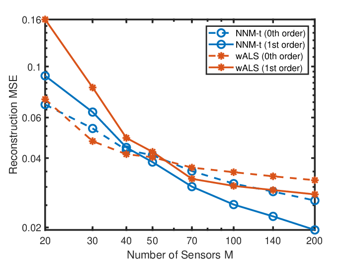
We evaluate the performance of the proposed schemes over different interpolation models under different number of measurement samples. For both NNM-t and wALS schemes, the zeroth order interpolation (12) and first order interpolation (13) are used to construct . In a single source propagation map, , and for , Fig. 5 shows that when there are only a few measurements, the methods based on zeroth order interpolation attain a smaller MSE than their counterparts based on first order models. This is because zeroth order models have less parameters to estimate. On the other hand, for medium to large number of measurements, methods based on first order interpolation perform better, because first order interpolation can substantially eliminate the bias in the local interpolation as revealed in our asymptotic analysis stated in Theorems 3 and 4.
V-B Performance under Different Shadowing Parameters
We quantify the propagation map reconstruction performance of the proposed schemes under different shadowing parameters. The simulations are performed under meters and separately with the baselines are Universal Kriging and k-LP. The experiment results shown in Fig. 6 reveal that the increasing of shadowing variance decreases the performance of all baselines. The larger the correlation distance, the better the performance.
V-C Performance under Different Measurements
We quantify the propagation map reconstruction performance of the proposed schemes under different number of measurements with fixed resolution and number of sources .
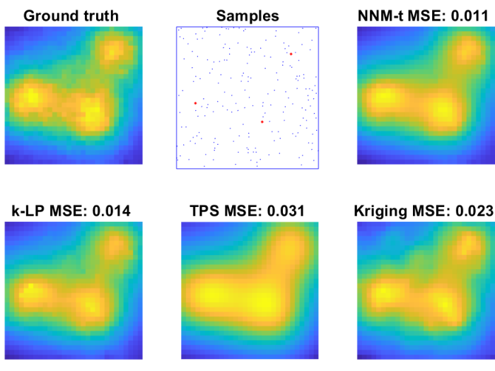
Fig. 7 demonstrates the reconstruction MSE versus the number of sensors . A visual plot of a realization of the propagation field, sampling pattern, and the reconstruction results under are demonstrated in Fig. 8. It is observed that the proposed NNM-t method can realize 10%–50% MSE reduction from all baseline schemes under medium to large , which translates to a saving of roughly of sensor measurements at a medium . At small , i.e., , its performance is similar to that of the TPS scheme. The NNM-t (adaptive) method works better than the NNM-t method and outperforms all baseline schemes because it optimizes the window size parameter for each grid cell in an adaptive way. The Universal Kriging and k-LP schemes perform well at a large , but their performance degrades at small , whereas, the TPS scheme works well at small , but suffers from substantial performance degradation at large . Finally, the On-grid LRMC scheme performs badly because the number of observations – is substantially smaller than the total number of entries to be recovered, and the matrix is likely non-identifiable in this regime.
Table I summarizes the computation time based on our implementation using Matlab. The Universal Kriging baseline is implemented by the “mGstat” function provided in the Geostatistical toolbox in Matlab. The NNM-t problem is solved by CVX using an interior point method. The complexity of k-LP and LRMC schemes is for benchmarking because they are the building blocks of the proposed NNM-t. As observed in Table I, the proposed method has a lower complexity than Universal Kriging at medium to large as expected from our analysis.
| 40 | 100 | 160 | 220 | 280 | 340 | 400 | |
|---|---|---|---|---|---|---|---|
| k-LP | 0.39 | 0.53 | 0.79 | 1.19 | 1.64 | 1.85 | 2.05 |
| LRMC | 6.63 | 6.39 | 6.60 | 6.76 | 6.45 | 7.11 | 6.91 |
| U-Kriging | 2.51 | 5.77 | 10.63 | 19.49 | 28.32 | 40.37 | 55.76 |
| NNM-t | 8.26 | 6.10 | 6.67 | 8.57 | 6.72 | 6.98 | 8.73 |
The gain of the proposed method over a pure interpolation scheme can be interpreted from the following two aspects. First, although there is shadowing, the matrix of the propagation field is still relatively low rank when choosing a large for the matrix dimension. In addition, the proposed NNM-t method can dynamically adjust the windows size such that there will always be enough observations to guarantee the recoverability of the matrix completion. Second, a pure interpolation method suffers from performance loss in the regions where measurements are locally too sparse, typically, at the edge of the area of interest. By contrast, the proposed interpolation assisted matrix completion approach can fill in the missing values in these regions using the global information constructed from the other part of the propagation field.
V-D Application in RSS-based Source Localization
Based on the reconstructed propagation map, we demonstrate the application of propagation map reconstruction under NNM-t for to RSS-based source localization. The localization algorithm based on matrix factorization developed in [2] is adopted. Specifically, based on the reconstructed propagation map matrix , the dominant singular vectors and of are computed. Then, the coordinates of the source are estimated via peak localization of the dominant singular vectors and [2].
Three baseline schemes for localization are evaluated. Baseline : WCL [28], we use to estimate the location of the source, where serves as the weight. Baseline : naive method, the location of the source is chosen as the location of the sensor with largest measurements. Baseline 3: Fingerprinting [48], the propagation map is first constructed using the Delaunay triangulation, and then, the location with the largest RSS in the reconstructed propagation map is selected as the location estimate of the source.
Fig. 9 shows the RMSE of RSS-based source localization based on the propagation map reconstructed from the proposed NNM-t method. The RMSE is reduced by roughly a half and both baseline schemes require times more sensors to achieve the same localization accuracy.

(a) (b)
V-E Experiment on a Real Dataset
We extend the experiment to a real dataset [49]. In this dataset, there are RSS measurements for each emitter. The measurements are taken in a indoor area. In the implementation of the proposed algorithm, the area is divided into grid cells such that the measurements are in the grid center. Among the measurements, – 140 measurements are randomly selected for reconstructing the prorogation field. The results in reconstruction MSE are reported in Fig. 10. It is shown that the proposed NNM-t method also achieves a promising performance on a real dataset.
VI Conclusion
In this paper, an interpolation assisted matrix completion method is proposed to reconstruct a propagation map from a sparse set of signal strength measurements. The observation matrix is enriched through interpolation and the bias and variance of the interpolation method are analyzed to build uncertainty-aware matrix completion algorithms which integrate interpolation with matrix completion. Furthermore, a minimum MSE method to optimize the window size for local interpolation is proposed. The numerical results demonstrate that the reconstruction MSE of the propagation map can be reduced by %–% compared to the state-of-the-art schemes which corresponds to a saving of nearly half of measurements under a not-so-dense sampling. In the application of RSS-based source localization, the RMSE of localization is reduced by more than % from a WCL baseline.
Appendix A Proof of Theorem 1
Applying first-order Taylor’s expansion to at the neighborhood of , the observation model in (2) becomes
| (29) |
due to the first order differentiability of .
Recall that , and therefore, . The expectation of the zeroth order solution in (12) can be written as
| (30) |
where in the last equation is due to the fact that as since we are only interested in the th grid such that according to the interpolation strategy.
As a result, the bias
So, , since from the observation model in (2). The results in Theorem 1 are thus proven.
Appendix B Proof of Theorem 2
Applying second order Taylor’s expansion to at the neighborhood of , we have
| (31) | ||||
where is the Hessian matrix of evaluated at point .
Denote . Then the expression in (31) can be rearranged into the following matrix form
| (32) |
where is a vector of the residual terms . Noticing that the residual from the Taylor’s expansion scales as with a bound due to the interpolation strategy, thus we have as . Therefore, .
From the measurement model (2), we have , where . The expectation of the first order solution in (13) can be written as
| (33) |
since the noise has zero mean, where .
Substitute in (33) with (32), the expectation of can be rewritten as
As a result, the bias
where the operation returns the th entry of a matrix .
The variance of can be derived following
Since is deterministic, , therefore
As a result,
Appendix C Proof of Theorem 3
The observation model in (2) can be rewritten as
| (34) | ||||
From (34), we have
| (35) |
where in the rest of the proof, the three terms in (35) are respectively denoted as
| (36) |
which serves as an approximation of the sensor density at point ,
| (37) |
which quantifies the weighted average bias of the estimate at location , and
| (38) |
which quantifies the weighted average error due to the measurement noise.
Then, dividing on both sides of (35) and according to the zeroth order solution (12), it yields
which implies that the error equals to
| (39) |
To analyze and , we derive the following lemmas.
Lemma 1.
Suppose that is second order differentiable and bounded. Then, for a sufficiently small ,
In addition, for a function that satisfies as uniformly for all there is
as for all , where .
Proof.
Let . Note that . We have
| (40) |
Consider the first order Taylor’s expansion
| (41) |
where is the first order derivative of , is the remainder term that satisfies as uniformly for all with due to the Taylor’s theorem and the fact that is second order differentiable. Thus,
| (42) | ||||
| (43) | ||||
| (44) |
where the second term in (42) equals , since due to (8). For (43), since the support of is , we have
| (45) |
which converges to because the term uniformly converges to and the integral term is bounded.
Define a random variable , where recall that . Then, using Lemma 1, the random variable can be shown to have the following property.
Lemma 2.
The mean and variance of are given by and
Proof.
Since and is independent of the term , it follows that
Moreover,
| (46) |
where the last equation is from Lemma 1. ∎
Define a random variable . We show the property of as follows.
Lemma 3.
The random variable has mean and its variance satisfies as where and .
Proof.
Let . We have
| (47) | ||||
Consider the first order Taylor expansion of as (41) and the second order Taylor expansion
We have
| (48) |
Recall that has a bounded support and the terms and uniformly converge to as due to the Taylor expansion. Then, the terms involving and from expanding the product in (48) are due to Lemma 1. As a result, equation (48) simplifies to
| (49) |
Thus, multiply (49) with , we obtain
| (50) |
Similarly,
| (51) | ||||
and thus, , as ∎
Next, it is observed that . This is because that due to the independence between the zero mean noise and . As a result, due to from Lemma 2. Therefore, .
In addition, from (37) and (38), it is observed that where the variable is i.i.d., since both and are i.i.d.. As a result, the law of large number implies as
In addition, the central limit theorem yields
as , where and as shown before.
References
- [1] D. Zhu, X. Peng, and G. Li, “A matrix completion based method for RFI source localization in microwave interferometric radiometry,” IEEE Trans. Geosci. Remote Sens., vol. 59, no. 9, pp. 7588–7602, 2021.
- [2] J. Chen and U. Mitra, “Unimodality-constrained matrix factorization for non-parametric source localization,” IEEE Trans. Signal Process., vol. 67, no. 9, pp. 2371–2386, May 2019.
- [3] D. Romero, S.-J. Kim, G. B. Giannakis, and R. López-Valcarce, “Learning power spectrum maps from quantized power measurements,” IEEE Trans. Signal Process., vol. 65, no. 10, pp. 2547–2560, 2017.
- [4] X. Mo, Y. Huang, and J. Xu, “Radio-map-based robust positioning optimization for uav-enabled wireless power transfer,” IEEE Wireless Commun. Letters, vol. 9, no. 2, pp. 179–183, 2019.
- [5] S. Chouvardas, S. Valentin, M. Draief, and M. Leconte, “A method to reconstruct coverage loss maps based on matrix completion and adaptive sampling,” in Proc. IEEE Int. Conf. Acoustics, Speech, and Signal Processing, 2016, pp. 6390–6394.
- [6] B. Fuchs, L. Le Coq, and M. D. Migliore, “On the interpolation of electromagnetic near field without prior knowledge of the radiating source,” IEEE Trans. Antennas Propag., vol. 65, no. 7, pp. 3568–3574, 2017.
- [7] A. C. M. Austin and M. J. Neve, “Efficient field reconstruction using compressive sensing,” IEEE Trans. Antennas Propag., vol. 66, no. 3, pp. 1624–1627, 2018.
- [8] S. G. Sathyanarayana, Z. Wang, N. Sun, B. Ning, S. Hu, and J. A. Hossack, “Recovery of blood flow from undersampled photoacoustic microscopy data using sparse modeling,” IEEE Trans. Med. Imag., vol. 41, no. 1, pp. 103–120, 2022.
- [9] Z. Ke, W. Huang, Z.-X. Cui, J. Cheng, S. Jia, H. Wang, X. Liu, H. Zheng, L. Ying, Y. Zhu, and D. Liang, “Learned low-rank priors in dynamic MR imaging,” IEEE Trans. Med. Imag., vol. 40, no. 12, pp. 3698–3710, 2021.
- [10] J. Chen, T. Li, J. Wang, and C. W. d. Silva, “WSN sampling optimization for signal reconstruction using spatiotemporal autoencoder,” IEEE Sensors Journal, vol. 20, no. 23, pp. 14 290–14 301, 2020.
- [11] Z. Liu, P. Wu, S. Duan, W. Zhan, X. Ma, and Y. Wu, “Spatiotemporal reconstruction of land surface temperature derived from fengyun geostationary satellite data,” IEEE J.. Sel. Topics Appl. Earth Observ., vol. 10, no. 10, pp. 4531–4543, 2017.
- [12] K. Sato and T. Fujii, “Kriging-based interference power constraint: Integrated design of the radio environment map and transmission power,” IEEE Trans. Cogn. Commun. Netw., vol. 3, no. 1, pp. 13–25, 2017.
- [13] A. Yakhot, T. Anor, and G. E. Karniadakis, “A reconstruction method for gappy and noisy arterial flow data,” IEEE Trans. Med. Imag., vol. 26, no. 12, pp. 1681–1697, 2007.
- [14] Y. Teganya, D. Romero, L. M. L. Ramos, and B. Beferull-Lozano, “Location-free spectrum cartography,” IEEE Trans. Signal Process., vol. 67, no. 15, pp. 4013–4026, 2019.
- [15] J. A. Bazerque and G. B. Giannakis, “Nonparametric basis pursuit via sparse kernel-based learning: A unifying view with advances in blind methods,” IEEE Signal Process. Mag., vol. 30, no. 4, pp. 112–125, 2013.
- [16] Y.-Q. Xu, B. Zhang, X. Zhang, J. Hu, and D. Guo, “Radio environment map construction with Gaussian process and kernel transformation,” in in Proc. IEEE Int. Conf. Commun., Image and Signal Processing, 2021, pp. 350–355.
- [17] M. Hamid and B. Beferull-Lozano, “Non-parametric spectrum cartography using adaptive radial basis functions,” in Proc. IEEE Int. Conf. Acoustics, Speech, and Signal Processing, 2017, pp. 3599–3603.
- [18] S.-J. Kim and G. B. Giannakis, “Cognitive radio spectrum prediction using dictionary learning,” in Proc. IEEE Global Telecomm. Conf., 2013, pp. 3206–3211.
- [19] A. Balachandrasekaran, A. L. Cohen, O. Afacan, S. K. Warfield, and A. Gholipour, “Reducing the effects of motion artifacts in fMRI: A structured matrix completion approach,” IEEE Trans. Med. Imag., vol. 41, no. 1, pp. 172–185, 2022.
- [20] M. D. Migliore, “A compressed sensing approach for array diagnosis from a small set of near-field measurements,” IEEE Trans. Antennas Propag., vol. 59, no. 6, pp. 2127–2133, 2011.
- [21] H. Sun and J. Chen, “Grid optimization for matrix-based source localization under inhomogeneous sensor topology,” in Proc. IEEE Int. Conf. Acoustics, Speech, and Signal Processing, 2021, pp. 5110–5114.
- [22] G. Zhang, X. Fu, J. Wang, X.-L. Zhao, and M. Hong, “Spectrum cartography via coupled block-term tensor decomposition,” IEEE Trans. Signal Process., vol. 68, pp. 3660–3675, 2020.
- [23] X. Wang, X. Wang, S. Mao, J. Zhang, S. C. Periaswamy, and J. Patton, “Deepmap: Deep Gaussian process for indoor radio map construction and location estimation,” in Proc. IEEE Global Telecomm. Conf. IEEE, 2018, pp. 1–7.
- [24] Y. Teganya and D. Romero, “Deep completion autoencoders for radio map estimation,” IEEE Trans. on Wireless Commun., 2021.
- [25] R. Levie, Ç. Yapar, G. Kutyniok, and G. Caire, “RadioUNet: Fast radio map estimation with convolutional neural networks,” IEEE Trans. on Wireless Commun., vol. 20, no. 6, pp. 4001–4015, 2021.
- [26] S. Shrestha, X. Fu, and M. Hong, “Deep spectrum cartography: Completing radio map tensors using learned neural models,” IEEE Trans. Signal Process., vol. 70, pp. 1170–1184, 2022.
- [27] H. Sun and J. Chen, “Regression assisted matrix completion for reconstructing a propagation field with application to source localization,” in Proc. IEEE Int. Conf. Acoustics, Speech, and Signal Processing, Singapore, May 2022, pp. 3353–3357.
- [28] J. Wang, P. Urriza, Y. Han, and D. Cabric, “Weighted centroid localization algorithm: theoretical analysis and distributed implementation,” IEEE Trans. Wireless Commun., vol. 10, no. 10, pp. 3403–3413, 2011.
- [29] E. J. Candes and Y. Plan, “Matrix completion with noise,” Proceedings of the IEEE, vol. 98, no. 6, pp. 925–936, 2010.
- [30] G. Tang and A. Nehorai, “Lower bounds on the mean-squared error of low-rank matrix reconstruction,” IEEE Trans. Signal Process., vol. 59, no. 10, pp. 4559–4571, 2011.
- [31] D. Zachariah, M. Sundin, M. Jansson, and S. Chatterjee, “Alternating least-squares for low-rank matrix reconstruction,” IEEE Signal Process. Lett., vol. 19, no. 4, pp. 231–234, Apr 2012.
- [32] S. Foucart and H. Rauhut, “An invitation to compressive sensing,” in A mathematical introduction to compressive sensing. Springer, 2013, pp. 1–39.
- [33] J. Fan, Local polynomial modelling and its applications: Monographs on statistics and applied probability 66. Routledge, 1996.
- [34] S. Boyd, S. P. Boyd, and L. Vandenberghe, Convex optimization. Cambridge university press, 2004.
- [35] D. Ruppert and M. P. Wand, “Multivariate locally weighted least squares regression,” The annals of statistics, vol. 22, no. 3, pp. 1346–1370, 1994.
- [36] A. Vehtari, A. Gelman, and J. Gabry, “Practical bayesian model evaluation using leave-one-out cross-validation and waic,” Statistics and computing, vol. 27, no. 5, pp. 1413–1432, 2017.
- [37] L. Brekhovskikh and Y. P. Lysanov, Fundamentals of ocean acoustics. Acoustical Society of America, 2004.
- [38] E. Candes and B. Recht, “Exact matrix completion via convex optimization,” Commun. of the ACM, vol. 55, no. 6, pp. 111–119, 2012.
- [39] D. L. Pimentel-Alarcón, N. Boston, and R. D. Nowak, “A characterization of deterministic sampling patterns for low-rank matrix completion,” IEEE J. Sel. Top. Signal Process., vol. 10, no. 4, pp. 623–636, 2016.
- [40] Y. Chen, Y. Chi, J. Fan, C. Ma, and Y. Yan, “Noisy matrix completion: Understanding statistical guarantees for convex relaxation via nonconvex optimization,” SIAM journal on optimization, vol. 30, no. 4, pp. 3098–3121, 2020.
- [41] Y. Chen, S. Bhojanapalli, S. Sanghavi, and R. Ward, “Completing any low-rank matrix, provably,” J. Mach. Learn. Res., vol. 16, no. 1, pp. 2999–3034, 2015.
- [42] P. Jain and P. Netrapalli, “Fast exact matrix completion with finite samples,” in Conference on Learning Theory. PMLR, 2015, pp. 1007–1034.
- [43] B. V. Srinivasan, R. Duraiswami, and R. Murtugudde, “Efficient kriging for real-time spatio-temporal interpolation,” in Proceedings of the 20th Conference on Probability and Statistics in the Atmospheric Sciences. American Meteorological Society Atlanta GA, 2010, pp. 228–235.
- [44] M. Stojanovic and J. Preisig, “Underwater acoustic communication channels: Propagation models and statistical characterization,” IEEE Commun. Mag., vol. 47, no. 1, pp. 84–89, 2009.
- [45] V.-P. Chowdappa, C. Botella, J. J. Samper-Zapater, and R. J. Martinez, “Distributed radio map reconstruction for 5G automotive,” IEEE Intell. Transp. Syst. Mag., vol. 10, no. 2, pp. 36–49, 2018.
- [46] A. Verdin, C. Funk, B. Rajagopalan, and W. Kleiber, “Kriging and local polynomial methods for blending satellite-derived and gauge precipitation estimates to support hydrologic early warning systems,” IEEE Trans. Geosci. Remote Sens., vol. 54, no. 5, pp. 2552–2562, 2016.
- [47] J. A. Bazerque, G. Mateos, and G. B. Giannakis, “Group-lasso on splines for spectrum cartography,” IEEE Trans. Signal Process., vol. 59, no. 10, pp. 4648–4663, 2011.
- [48] J. Talvitie, M. Renfors, and E. S. Lohan, “Distance-based interpolation and extrapolation methods for RSS-based localization with indoor wireless signals,” IEEE Trans. Veh. Technol., vol. 64, no. 4, pp. 1340–1353, 2015.
- [49] T. King, S. Kopf, T. Haenselmann, C. Lubberger, and W. Effelsberg, “CRAWDAD dataset mannheim/compass (v. 2008-04-11),” Downloaded from https://crawdad.org/mannheim/compass/20080411/signalstrength, Apr. 2008, traceset: signalstrength.
- [50] E. Parzen, “On estimation of a probability density function and mode,” The annals of mathematical statistics, vol. 33, no. 3, pp. 1065–1076, 1962.
- [51] A. DasGupta, Asymptotic theory of statistics and probability. Springer, 2008, vol. 180.
![[Uncaptioned image]](2207.13473v2/Bios/haosun.jpg) |
Hao Sun received the B.S. degree in biomedical engineering from the University of Electronic Science and Technology of China (UESTC), Chengdu, China, in 2018. He received two national scholarships during his undergraduate study. He is currently working toward the Ph.D. degree with the School of Science and Engineering and the Future Network of Intelligence Institute (FNii) at the Chinese University of Hong Kong, Shenzhen (CUHK-Shenzhen), Guangdong, China. He works on matrix completion and tensor decomposition with application to radio map reconstruction and source localization. |
![[Uncaptioned image]](2207.13473v2/juntingchen.png) |
Junting Chen (S’11–M’16) received the Ph.D. degree in Electronic and Computer Engineering from the Hong Kong University of Science and Technology (HKUST), Hong Kong SAR China, in 2015, and the B.Sc. degree in Electronic Engineering from Nanjing University, Nanjing, China, in 2009. From 2014–2015, he was a visiting student with the Wireless Information and Network Sciences Laboratory at MIT, Cambridge, MA, USA. He is an Assistant Professor with the School of Science and Engineering and the Future Network of Intelligence Institute (FNii) at the Chinese University of Hong Kong, Shenzhen (CUHK-Shenzhen), Guangdong, China. Prior to joining CUHK-Shenzhen, he was a Postdoctoral Research Associate with the Ming Hsieh Department of Electrical Engineering, University of Southern California (USC), Los Angeles, CA, USA, from 2016–2018, and with the Communication Systems Department of EURECOM, Sophia-Antipolis, France, from 2015–2016. He was a recipient of the HKTIIT Post-Graduate Excellence Scholarships in 2012 from HKUST. He works on unimodal signal processing, radio map sensing, UAV assisted communications, and, more generally, machine learning and optimization for wireless communications and localization. |