跳到论文正文
W Papers独立论文阅读器 arXiv:2207.13435 论文正文 计算阅读时间 · 0%
引用这篇论文根据当前论文元数据生成,正式投稿前建议核对。


License: CC BY 4.0
arXiv:2207.13435v1 [gr-qc] 27 Jul 2022

Analytically Approximation Solution to Einstein-Cubic Gravity

S. N. Sajadi Thanks: Electronic address: naseh.sajadi@gmail.com    S. H. Hendi Thanks: Electronic address: hendi@shirazu.ac.ir Affiliation: Department of Physics, School of Science, Shiraz University, Shiraz 71454, Iran Affiliation: Biruni Observatory, School of Science, Shiraz University, Shiraz 71454, Iran Affiliation: Canadian Quantum Research Center 204-3002 32 Ave Vernon, BC V1T 2L7 Canada
Abstract

In this work, we introduce analytical approximate black hole solutions in Einstein-Cubic gravity. To obtain complete solutions, we construct the the near horizon and asymptotic solutions as the first step. Then, the approximate analytic solutions are obtained through continued-fraction expansion. We also compute the thermodynamic quantities and use the first law and Smarr formula to obtain the analytic solutions for near horizon quantities. Finally, we follow the same approach to obtain the new static black hole solutions with different metric functions.

1 Introduction

Higher-order gravity models recently attracted considerable attention. In the context of cosmology, in order to go beyond the standard Λ\LambdaCDM model and find an explanation for the late-time accelerated expansion, dark matter or inflation [1]-[4], higher-order curvature gravity theories are helpful. In AdS/CFT context, higher-order gravities have been used as tools to characterize numerous properties of strongly coupled conformal field theories [5]-[10]. From quantum gravity viewpoint, in order to unify quantum mechanics and gravitational interactions, going beyond the Einstein gravity is necessary [11].

In recent years, a new class of higher derivative theories has been discovered that is ghost-free and in four dimensions neither topological nor trivial known as Generalized Quasi-Topological Gravity [12]-[15]. One of the such higher-derivative gravity theories which in the four dimensions is neither topological nor trivial is Einsteinian cubic gravity. This theory of gravity, that has been recently proposed in [16], is the most general up to cubic order in curvature dimension independent theory of gravity that shares its graviton spectrum with Einstein’s theory on constant curvature backgrounds. The Einsteinian cubic gravity field equations admit generalizations of the Schwarzschild solution, i.e. static, spherically symmetric solutions with a single metric function [17, 18, 19]. The Lagrangian density of this theory is given by [17, 20]

L=R−2​Λ+β1​κ4+β2​κ6+α​P,L=R-2\Lambda+\beta_{1}\kappa_{4}+\beta_{2}\kappa_{6}+\alpha P,

where κ4\kappa_{4} and κ6\kappa_{6} are four and six-dimensional Euler densities and correspond to the usual Lovelock terms, and PP is the cubic term. In 4-dimensions the terms proportional to β1\beta_{1} and β2\beta_{2} have no contribution on the field equations. In [17]-[21], the authors construct static and spherically symmetric generalizations of the Schwarzschild and Reissner-Nordström-(Anti-)de Sitter black-hole solutions in four-dimensions and study the orbit of massive test bodies near a black hole, especially computing the innermost stable circular orbit. They compute constraints on the ECG coupling parameter and the shadow of an ECG black hole. In [22], bounce universe in the critical point of the coupling constants of the theory has been studied. In [23], the holographic complexity of AdS black hole in Einsteinian cubic gravity has been investigated through the ”complexity equals action” and ”complexity equals volume” conjectures. In [24] the condensation of a charged scalar field in a (3 + 1)-dimensional asymptotically AdS background in the context of Einsteinian cubic gravity has been studied. In [25] holography on squashed-spheres, in [27] the holographic entanglement entropy, and in [27] various aspects of holographic ECG have been studied. In [20], the gravitational lensing due to the presence of supermassive black holes at the center of the Milky Way and other galaxies in Einsteinian Cubic Gravity has been studied.

In this paper, by using the continued fraction expansion technique, we obtain the static spherically symmetric solutions for the theory. This ansatz is designed so that the coefficients in the continued fraction are fixed by the behavior of the metric near the event horizon, while the pre-factors are introduced to match the asymptotic behavior at infinity [28],[29],[30]. This method is an accurate analytic method that has recently been applied with success in a variety of contexts [31],[32]. These analytic studies of the black hole also allowed us to study thermodynamics and other properties of the solutions. While, the numerical solutions do not give a clear picture of the metric dependence on physical parameters of the system.

The paper is organized as follows: In the next section, we first review Einsteinian cubic gravity and continued-fraction expansion. Then, calculating the thermodynamical quantities and inserting them in the first law and Smarr formula, we obtain the solutions for the near horizon quantities. We also plotted the metric functions and thermodynamical quantities and compared them with the previous works on this theory, we find a good agreement between them. In Sec. 3, we introduce new solutions of the theory with different metric functions. Finally, we conclude the paper in Sec. (4).

2 Basic equations

In 4D, Einstein cubic gravity theory is determined by the action [17]-[21]

𝒮=116​π​G​∫d4​x​−g​(R−2​Λ+α​P−κ​Fa​b​Fa​b),\mathcal{S}=\dfrac{1}{16\pi G}\int d^{4}x\sqrt{-g}(R-2\Lambda+\alpha P-\kappa F_{ab}F^{ab}), (1)

where RR represent the Ricci scalar, α\alpha is coupling constant of the theory, and PP cubic-in-curvature correction to the Einstein-Hilbert action is given as [17]-[21]

P=12RacbdRcedfReafb+Ra​bc​dRc​de​fRe​fa​b−12Ra​b​c​dRa​cRb​d+8RabRbcRca.P=12R_{a}{}^{c}{}_{b}{}^{d}R_{c}{}^{e}{}_{d}{}^{f}R_{e}{}^{a}{}_{f}{}^{b}+R_{ab}{}^{cd}R_{cd}{}^{ef}R_{ef}{}^{ab}-12R_{abcd}R^{ac}R^{bd}+8R_{a}{}^{b}R_{b}{}^{c}R_{c}{}^{a}. (2)

The correction term in four dimensions is dynamical and is not topological or trivial [17]-[21]. Using the variational principle, one can find the following equation of motion

Ea​b\displaystyle E_{ab} =Pa​c​d​eRbc​d​e−12ga​bL−2∇c∇dPa​c​d​b−2Ta​b=0,\displaystyle=P_{acde}R_{b}{}^{cde}-\dfrac{1}{2}g_{ab}L-2\nabla^{c}\nabla^{d}P_{acdb}-2T_{ab}=0,
∇aFa​b\displaystyle\nabla_{a}F^{ab} =0,Ta​b=Fd​a​Fbd−14​ga​b​Fd​e​Fd​e\displaystyle=0,\;\;\;\;\;\;\;T_{ab}=F_{da}F^{d}_{b}-\dfrac{1}{4}g_{ab}F_{de}F^{de} (3)

where LL is the Lagrangian of Einstein cubic gravity and Pa​b​c​d=∂L/∂Ra​b​c​dP^{abcd}=\partial L/\partial R_{abcd} is

Pa​b​c​d\displaystyle P_{abcd} =ga[cgb]d+6α[Ra​dRb​c−Ra​cRb​d+gb​dRaeRc​e−ga​dRbeRc​e−gb​cRaeRd​e+ga​cRbeRd​e\displaystyle=g_{a[c}\;g_{b]d}+6\alpha[R_{ad}R_{bc}-R_{ac}R_{bd}+g_{bd}R_{a}^{e}R_{ce}-g_{ad}R_{b}^{e}R_{ce}-g_{bc}R_{a}^{e}R_{de}+g_{ac}R_{b}^{e}R_{de}
−gb​d​Re​f​Ra​e​c​f+gb​c​Re​f​Ra​e​d​f+ga​d​Re​f​Rb​e​c​f−3​Ra​Rb​e​c​fdef−ga​c​Re​f​Rb​e​d​f+3​Ra​Rb​e​d​fcef\displaystyle-g_{bd}R^{ef}R_{aecf}+g_{bc}R^{ef}R_{aedf}+g_{ad}R^{ef}R_{becf}-3R_{a}{}^{e}{}_{d}{}^{f}R_{becf}-g_{ac}R^{ef}R_{bedf}+3R_{a}{}^{e}{}_{c}{}^{f}R_{bedf}
+12Ra​bRc​d​e​fe​f].\displaystyle+\dfrac{1}{2}R_{ab}{}^{ef}R_{cdef}]. (4)

Here, we consider the following spherically symmetric and static line element for describing the geometry of spacetime

d​s2=−f⁡(r)​d​t2+d​r2f⁡(r)+r2​(d​θ2+sin2⁡(k​θ)k​d​ϕ2).ds^{2}=-f(r)dt^{2}+\dfrac{dr^{2}}{f(r)}+r^{2}\left(d\theta^{2}+\dfrac{\sin^{2}(\sqrt{k}\theta)}{k}d\phi^{2}\right). (5)

As, we know generic static, spherically symmetric metrics do not need obey gt​t​gr​r=−1g_{tt}g_{rr}=-1 necessarily, but field equation (2) admits solutions with this property [17]-[21], to which case we shall restrict our consideration in this section.

By inserting the metric into the field equations, the differential equations for f⁡(r)f(r) become

Err−2​Trr\displaystyle E^{r}_{r}-2T^{r}_{r} =14​r5[24αr2ff′′′(2k−2f+rf′)+24αr3ff′′2+r(r4+12αrff′−96kαf+96αf2)f′′\displaystyle=\dfrac{1}{4r^{5}}[24\alpha r^{2}ff^{\prime\prime\prime}(2k-2f+rf^{\prime})+24\alpha r^{3}ff^{\prime\prime 2}+r(r^{4}+12\alpha rff^{\prime}-96k\alpha f+96\alpha f^{2})f^{\prime\prime}
+24αr(4f−k)f′2+4r3(−k+f+Λr2)+(96kαf+6r4−96αf2)f′]+q2r4=0,\displaystyle+24\alpha r(4f-k)f^{\prime 2}+4r^{3}(-k+f+\Lambda r^{2})+(96k\alpha f+6r^{4}-96\alpha f^{2})f^{\prime}]+\dfrac{q^{2}}{r^{4}}=0, (6)

Expanding the function f⁡(r)f(r) around the event horizon r+r_{+}

f⁡(r)\displaystyle f(r) =f1​(r−r+)+f2​(r−r+)2+f3​(r−r+)3+…\displaystyle=f_{1}(r-r_{+})+f_{2}(r-r_{+})^{2}+f_{3}(r-r_{+})^{3}+... (7)

and then inserting these expressions into equations (2), we find

f2\displaystyle{f_{2}} =−2​Λ​r+4+2​k​r+2+12​α​k​f12−3​f1​r+2−2​q2r+4,\displaystyle=\dfrac{-2\Lambda r_{+}^{4}+2kr_{+}^{2}+12\alpha kf_{1}^{2}-3f_{1}r_{+}^{2}-2q^{2}}{r_{+}^{4}},
f3\displaystyle{f_{3}} =13​r+5+72​α​r+3​f12+144​α​r+2​f1​k[−6f2r+4+f1r+3(1−48αf22)+4r+2(24αf12f2−k)\displaystyle=\dfrac{1}{3r_{+}^{5}+72\alpha r_{+}^{3}f_{1}^{2}+144\alpha r_{+}^{2}f_{1}k}[-6f_{2}r_{+}^{4}+f_{1}r_{+}^{3}(1-48\alpha f_{2}^{2})+4r_{+}^{2}(24\alpha f_{1}^{2}f_{2}-k)
+48αf1r+(−f12+3kf2)+8q2−96αkf12],\displaystyle+48\alpha f_{1}r_{+}(-f_{1}^{2}+3kf_{2})+8q^{2}-96\alpha kf_{1}^{2}],
f4\displaystyle f_{4} =−1r+6​(96​α​f1​k+48​α​r+​f12+r+3)[20q2+144αkf2f3r+3+48αf23r+4−384αf1f23r+4\displaystyle=-\dfrac{1}{r_{+}^{6}(96\alpha f_{1}k+48\alpha r_{+}f_{1}^{2}+r_{+}^{3})}[20q^{2}+144\alpha kf_{2}f_{3}r_{+}^{3}+48\alpha f_{2}^{3}r_{+}^{4}-384\alpha f_{1}f_{2}^{3}r_{+}^{4}
−384​α​r+3​f1​f22+9​r+5​f3−4​r+4​f2−6​k​r+6−f1​r+3−360​α​k​f12+624​α​r+2​f2​f12−576​α​r+3​f12​f3\displaystyle-384\alpha r_{+}^{3}f_{1}f_{2}^{2}+9r_{+}^{5}f_{3}-4r_{+}^{4}f_{2}-6kr_{+}^{6}-f_{1}r_{+}^{3}-360\alpha kf_{1}^{2}+624\alpha r_{+}^{2}f_{2}f_{1}^{2}-576\alpha r_{+}^{3}f_{1}^{2}f_{3}
−240αr+f13−792αkr+2f1f3+504αf1f2f3r+4+720αr+kf1f2−144αr+2kf22]\displaystyle-240\alpha r_{+}f_{1}^{3}-792\alpha kr_{+}^{2}f_{1}f_{3}+504\alpha f_{1}f_{2}f_{3}r_{+}^{4}+720\alpha r_{+}kf_{1}f_{2}-144\alpha r_{+}^{2}kf_{2}^{2}] (8)

where r+r_{+}, f1f_{1} are undetermined constants of integration. In the large rr limit, we linearize the field equations about the Schwarzschild background

f⁡(r)=1−2​Mr+ϵ​F​(r)f(r)=1-\dfrac{2M}{r}+\epsilon F(r) (9)

where F⁡(r)F(r) should be calculated from the field equations. We linearize the differential equation by keeping terms only to order ϵ\epsilon, and the resulting differential equation for F⁡(r)F(r) takes the form

F′′′+γ⁡(r)​F′′+η⁡(r)​F′+ω⁡(r)​F+g⁡(r)=0F^{\prime\prime\prime}+\gamma(r)F^{\prime\prime}+\eta(r)F^{\prime}+\omega(r)F+g(r)=0 (10)

where

γ⁡(r)\displaystyle\gamma(r) =−96​α​r2+1152​α​M2−768​α​M​r−96​k​α​r2+r6+192​α​k​M​r48​α​r​(2​M−r)​(3​M−r+k​r),\displaystyle=-\dfrac{96\alpha r^{2}+1152\alpha M^{2}-768\alpha Mr-96k\alpha r^{2}+r^{6}+192\alpha kMr}{48\alpha r(2M-r)(3M-r+kr)}, (11)
η⁡(r)\displaystyle\eta(r) =−16​α​r2​k+416​α​M2−240​α​M​r+48​α​k​M​r+16​α​r2−r68​α​r2​(2​M−r)​(3​M−r+k​r),\displaystyle=\dfrac{-16\alpha r^{2}k+416\alpha M^{2}-240\alpha Mr+48\alpha kMr+16\alpha r^{2}-r^{6}}{8\alpha r^{2}(2M-r)(3M-r+kr)}, (12)
ω⁡(r)\displaystyle\omega(r) =−288​α​k​M​r−576​α​M​r+1680​α​M2+r612​α​r3​(2​M−r)​(3​M+k​r−r),\displaystyle=-\dfrac{288\alpha kMr-576\alpha Mr+1680\alpha M^{2}+r^{6}}{12\alpha r^{3}(2M-r)(3M+kr-r)}, (13)
g⁡(r)\displaystyle g(r) =(k−1)​r7−q2​r5−288​M​α​r2​(k−1)+120​α​M2​r​(5​k−14)+2208​α​M312​α​r4​(2​M−r)​(3​M−r+k​r).\displaystyle=\dfrac{(k-1)r^{7}-q^{2}r^{5}-288M\alpha r^{2}(k-1)+120\alpha M^{2}r(5k-14)+2208\alpha M^{3}}{12\alpha r^{4}(2M-r)(3M-r+kr)}. (14)

In the large rr limit and k=1k=1, the homogenous equation reads

F′′′+r4144​M​α​F′′+r324​M​α​F′+r236​M​α​F=0.F^{\prime\prime\prime}+\dfrac{r^{4}}{144M\alpha}F^{\prime\prime}+\dfrac{r^{3}}{24M\alpha}F^{\prime}+\dfrac{r^{2}}{36M\alpha}F=0. (15)

This equation can be solved exactly in terms of hypergeom functions

F⁡(r)\displaystyle F(r) =c1​hypergeom​([15],[35],−r5720​M​α)+c2​r2​hypergeom​([35],[75],−r5720​M​α)\displaystyle=c_{1}\text{hypergeom}\left(\left[\dfrac{1}{5}\right],\left[\dfrac{3}{5}\right],-\dfrac{r^{5}}{720M\alpha}\right)+c_{2}r^{2}\text{hypergeom}\left(\left[\dfrac{3}{5}\right],\left[\dfrac{7}{5}\right],-\dfrac{r^{5}}{720M\alpha}\right)
+c3​r​hypergeom​([25,1],[45,65],−r5720​M​α).\displaystyle+c_{3}r\text{hypergeom}\left(\left[\dfrac{2}{5},1\right],\left[\dfrac{4}{5},\dfrac{6}{5}\right],-\dfrac{r^{5}}{720M\alpha}\right). (16)

In tha large rr, F⁡(r)F(r) decays super-exponentially and can be neglected. More relevant is the particular solution, which reads

fp​(r)=\displaystyle f_{p}(r)= ∑n=2Fnrn=F2r2+F3r3+….\displaystyle\sum_{n=2}\dfrac{F_{n}}{r^{n}}=\dfrac{F_{2}}{r^{2}}+\dfrac{F_{3}}{r^{3}}+.... (17)

By inserting the above expansions into the field equations (10) and solving order by order, one can get

fp​(r)\displaystyle f_{p}(r) =q2r2+F4r4−432​α​M2r6+64​M​α​(23​M2+18​q2)3​r7−4656​M2​q2​α7​r8+432​M​α​F4r9\displaystyle=\dfrac{q^{2}}{r^{2}}+\dfrac{F_{4}}{r^{4}}-\dfrac{432\alpha M^{2}}{r^{6}}+\dfrac{64M\alpha(23M^{2}+18q^{2})}{3r^{7}}-\dfrac{4656M^{2}q^{2}\alpha}{7r^{8}}+\dfrac{432M\alpha F_{4}}{r^{9}}
−736​M2​F4​αr10−995328​M3​α25​r11+3456​M2​α2​(1831​M2+576​q2)11​r12+𝒪⁡(1r13).\displaystyle-\dfrac{736M^{2}F_{4}\alpha}{r^{10}}-\dfrac{995328M^{3}\alpha^{2}}{5r^{11}}+\dfrac{3456M^{2}\alpha^{2}(1831M^{2}+576q^{2})}{11r^{12}}+\mathcal{O}\left(\dfrac{1}{r^{13}}\right). (18)

For α\alpha goes to zero, one expects the metric returning to the RN. As a result F4F_{4} should be zero. The solution at large rr, thereby giving

f⁡(r)\displaystyle f(r) ≈1−2​Mr+q2r2−432​α​M2r6+64​M​α​(23​M2+18​q2)3​r7−4656​M2​q2​α7​r8−995328​M3​α25​r11\displaystyle\approx 1-\dfrac{2M}{r}+\dfrac{q^{2}}{r^{2}}-\dfrac{432\alpha M^{2}}{r^{6}}+\dfrac{64M\alpha(23M^{2}+18q^{2})}{3r^{7}}-\dfrac{4656M^{2}q^{2}\alpha}{7r^{8}}-\dfrac{995328M^{3}\alpha^{2}}{5r^{11}}
+3456​M2​α2​(1831​M2+576​q2)11​r12.\displaystyle+\dfrac{3456M^{2}\alpha^{2}(1831M^{2}+576q^{2})}{11r^{12}}. (19)

It should be noted, the other components of field equations give the same results for (7)-(2). We wish to obtain an approximate analytic solution (for k=1k=1) that is valid near the horizon and at large rr. To this end we employ a continued fraction expansion [31], and write

f⁡(r)=x​A​(x),x=1−r+rf(r)=xA(x),\hskip 28.45274ptx=1-\frac{r_{+}}{r} (20)

with

A⁡(x)\displaystyle A(x) =1−ϵ⁡(1−x)+(a0−ϵ)​(1−x)2+a1​(1−x)31+a2​x1+a3​x1+a4​x1+…\displaystyle=1-\epsilon(1-x)+(a_{0}-\epsilon)(1-x)^{2}+\dfrac{a_{1}(1-x)^{3}}{1+\dfrac{a_{2}x}{1+\dfrac{a_{3}x}{1+\dfrac{a_{4}x}{1+...}}}} (21)

where we truncate the continued fraction at order 44. By expanding (20) near the horizon (x→0x\to 0) and the asymptotic region (x→1x\to 1) we obtain

ϵ=−F1r+−1,a0=q2r+2,a1=−1−a0+2​ϵ+r+​f1\epsilon=-\dfrac{F_{1}}{r_{+}}-1,\qquad a_{0}=\dfrac{q^{2}}{r_{+}^{2}},\qquad a_{1}=-1-a_{0}+2\epsilon+r_{+}f_{1} (22)

for the lowest order expansion coefficients, with the remaining aia_{i} given in terms of (r+,f1)(r_{+},f_{1}); we provide these expressions in the Appendix A.

The result is an approximate analytic solution for metric functions everywhere outside the horizon. For a static space time we have a timelike Killing vector ξ=∂t\xi=\partial_{t} everywhere outside the horizon and so we obtain

T\displaystyle T =f′(r)4​π|r+=f14​π=(1−2​ϵ+a1+a0)4​π​r+=1+δ⁡(r+,q)4​π​r+.\displaystyle=\left.\dfrac{f^{{}^{\prime}}(r)}{4\pi}\right|_{r_{+}}=\dfrac{f_{1}}{4\pi}={\dfrac{(1-2\epsilon+a_{1}+a_{0})}{{4\pi r_{+}}}}=\dfrac{1+\delta(r_{+},q)}{4\pi r_{+}}. (23)

Extreme charged black hole solutions exist if f1=0f_{1}=0 implying that a1=2​ϵ−a0−1a_{1}=2\epsilon-a_{0}-1. We compute the entropy as follows [33], [34]

S=−2π∫H​o​r​i​z​o​nd2xηδ​Lδ​Ra​b​c​dϵa​bϵc​d\displaystyle S=-2\pi\int_{Horizon}d^{2}x\sqrt{\eta}\dfrac{\delta L}{\delta R_{abcd}}\epsilon_{ab}\epsilon_{cd} =A4​[1+6​α​(f′2r+2+4​f′r+3)]=A4​[1+6​α​(f12r+2+4​f1r+3)]\displaystyle=\dfrac{A}{4}\left[1+6\alpha\left(\dfrac{f^{\prime 2}}{r_{+}^{2}}+\dfrac{4f^{\prime}}{r_{+}^{3}}\right)\right]=\dfrac{A}{4}\left[1+6\alpha\left(\dfrac{f^{2}_{1}}{r_{+}^{2}}+\dfrac{4f_{1}}{r_{+}^{3}}\right)\right]
=A4​[1+6​α​(1+δ⁡(r+,q))r+4​[5+δ⁡(r+,q)]].\displaystyle=\dfrac{A}{4}\left[1+\dfrac{6\alpha(1+\delta(r_{+},q))}{r_{+}^{4}}[5+\delta(r_{+},q)]\right]. (24)

We now consider the thermodynamics of these black hole solutions, whose basic equations are the first law and Smarr formula

d​M=T​d​S+ϕ​d​q,dM=TdS+\phi dq, (25)
M=2​T​S+q​ϕ,M=2TS+q\phi, (26)

where there are no pressure/volume terms since we have set Λ=0\Lambda=0. From Eq. (26) we have

M=r+4+30​α+66​α​δ​(r+,q)+42​α​δ2​(r+,q)+r+4​δ​(r+,q)+6​α​δ3​(r+,q)+2​q2​r+22​r+2,M=\dfrac{r_{+}^{4}+30\alpha+66\alpha\delta(r_{+},q)+42\alpha\delta^{2}(r_{+},q)+r_{+}^{4}\delta(r_{+},q)+6\alpha\delta^{3}(r_{+},q)+2q^{2}r_{+}^{2}}{2r_{+}^{2}}, (27)

yielding the mass parameter as a function of the horizon radius. In the following, we show that the asymptotic behavior of the mass (27) is the same as the mass of the Schwarzschild black hole. So, one can interpret the mass (27), as ADM mass. We now impose the first law (25), which becomes

∂M∂r+​d​r++∂M∂q​d​q=T​∂S∂r+​d​r++T​∂S∂q​d​q+ϕ​d​q\dfrac{\partial M}{\partial r_{+}}dr_{+}+\dfrac{\partial M}{\partial q}dq=T\dfrac{\partial S}{\partial r_{+}}dr_{+}+T\dfrac{\partial S}{\partial q}dq+\phi dq (28)

yielding

∂M∂r+−T​∂S∂r+=0,⟹\displaystyle\dfrac{\partial M}{\partial r_{+}}-T\dfrac{\partial S}{\partial r_{+}}=0,\hskip 14.22636pt\Longrightarrow
60​α+132​α​δ​(r+,q)+84​α​δ2​(r+,q)+12​α​δ3​(r+,a)+2​q2​r+2−48​α​r+​∂δ⁡(r+,q)∂r+\displaystyle 60\alpha+132\alpha\delta(r_{+},q)+84\alpha\delta^{2}(r_{+},q)+12\alpha\delta^{3}(r_{+},a)+2q^{2}r_{+}^{2}-48\alpha r_{+}\dfrac{\partial\delta(r_{+},q)}{\partial r_{+}}
−60​α​r+​δ​(r+,q)​∂δ⁡(r+,q)∂r+−r+5​∂δ⁡(r+,q)∂r+−12​α​r+​δ2​(r+,q)​∂δ⁡(r+,q)∂r+=0\displaystyle-60\alpha r_{+}\delta(r_{+},q)\dfrac{\partial\delta(r_{+},q)}{\partial r_{+}}-r_{+}^{5}\dfrac{\partial\delta(r_{+},q)}{\partial r_{+}}-12\alpha r_{+}\delta^{2}(r_{+},q)\dfrac{\partial\delta(r_{+},q)}{\partial r_{+}}=0 (29)

and

∂M∂q−T​∂S∂q−ϕ=0,⟹\displaystyle\dfrac{\partial M}{\partial q}-T\dfrac{\partial S}{\partial q}-\phi=0,\hskip 14.22636pt\Longrightarrow
48​α​∂δ⁡(r+,q)∂q+60​α​δ​(r+,q)​∂δ⁡(r+,q)∂q+r+4​∂δ⁡(r+,q)∂q+12​α​δ2​(r+,q)​∂δ⁡(r+,q)∂q+2​q2​r+2=0\displaystyle 48\alpha\dfrac{\partial\delta(r_{+},q)}{\partial q}+60\alpha\delta(r_{+},q)\dfrac{\partial\delta(r_{+},q)}{\partial q}+r_{+}^{4}\dfrac{\partial\delta(r_{+},q)}{\partial q}+12\alpha\delta^{2}(r_{+},q)\dfrac{\partial\delta(r_{+},q)}{\partial q}+2q^{2}r_{+}^{2}=0 (30)

as differential equations that must be satisified by δ⁡(r+,q)\delta(r_{+},q). From now, we consider the case q=0q=0. So, from equation (2) one can get

r+4​(1+δ⁡(r+))2+24​α​(1+δ⁡(r+))3+6​α​(1+δ⁡(r+))4+4​c1​r+4=0,r_{+}^{4}(1+\delta(r_{+}))^{2}+24\alpha(1+\delta(r_{+}))^{3}+6\alpha(1+\delta(r_{+}))^{4}+4c_{1}r_{+}^{4}=0, (31)

by solving above equation one can obtain solutions for δ⁡(r+)\delta(r_{+}) as:

δ1,2\displaystyle\delta^{1,2} =−2+2​𝒰12​α​𝒬16±\displaystyle=-2+\dfrac{\sqrt{2\mathcal{U}}}{12\sqrt{\alpha}\mathcal{Q}^{\frac{1}{6}}}\pm
i​2α​𝒬16​𝒰14​864​2​𝒬​α32+𝒰​𝒬23​r++𝒰​(r+7+288​c1​α​r+3+𝒬13​(4​r+4−144​α))−36​2​α​𝒬​r+4\displaystyle\dfrac{i\sqrt{2}}{\sqrt{\alpha}\mathcal{Q}^{\frac{1}{6}}\mathcal{U}^{\frac{1}{4}}}\sqrt{864\sqrt{2\mathcal{Q}}\alpha^{\frac{3}{2}}+\sqrt{\mathcal{U}}\mathcal{Q}^{\frac{2}{3}}r_{+}+\sqrt{\mathcal{U}}(r_{+}^{7}+288c_{1}\alpha r_{+}^{3}+\mathcal{Q}^{\frac{1}{3}}(4r_{+}^{4}-144\alpha))-36\sqrt{2\alpha\mathcal{Q}}r_{+}^{4}} (32)
δ3,4\displaystyle\delta^{3,4} =−2+2​𝒰12​α​𝒬16±\displaystyle=-2+\dfrac{\sqrt{2\mathcal{U}}}{12\sqrt{\alpha}\mathcal{Q}^{\frac{1}{6}}}\pm
2α​𝒬16​𝒰14​864​2​𝒬​α32−𝒰​𝒬23​r+−𝒰​(r+7+288​c1​α​r+3+𝒬13​(4​r+4−144​α))−36​2​α​𝒬​r+4\displaystyle\dfrac{\sqrt{2}}{\sqrt{\alpha}\mathcal{Q}^{\frac{1}{6}}\mathcal{U}^{\frac{1}{4}}}\sqrt{864\sqrt{2\mathcal{Q}}\alpha^{\frac{3}{2}}-\sqrt{\mathcal{U}}\mathcal{Q}^{\frac{2}{3}}r_{+}-\sqrt{\mathcal{U}}(r_{+}^{7}+288c_{1}\alpha r_{+}^{3}+\mathcal{Q}^{\frac{1}{3}}(4r_{+}^{4}-144\alpha))-36\sqrt{2\alpha\mathcal{Q}}r_{+}^{4}} (33)

where

𝒫\displaystyle\mathcal{P} =36​2​α​c1​192​c1​α​r+8+373248​c1​α3+24​α​r+8−9216​α2​c12​r+4−20736​c1​α2​r+4\displaystyle=36\sqrt{2\alpha c_{1}}\sqrt{192c_{1}\alpha r_{+}^{8}+373248c_{1}\alpha^{3}+24\alpha r_{+}^{8}-9216\alpha^{2}c_{1}^{2}r_{+}^{4}-20736c_{1}\alpha^{2}r_{+}^{4}}
𝒬\displaystyle\mathcal{Q} =(−864​c1​r+4​α+31104​c1​α2+r+8+𝒫)​r+\displaystyle=(-864c_{1}r_{+}^{4}\alpha+31104c_{1}\alpha^{2}+r_{+}^{8}+\mathcal{P})r_{+}
𝒰\displaystyle\mathcal{U} =72​α​𝒬13−2​r+4​𝒬13+𝒬23​r++288​r+3​c1​α+r+7.\displaystyle=72\alpha\mathcal{Q}^{\frac{1}{3}}-2r_{+}^{4}\mathcal{Q}^{\frac{1}{3}}+\mathcal{Q}^{\frac{2}{3}}r_{+}+288r_{+}^{3}c_{1}\alpha+r_{+}^{7}. (34)

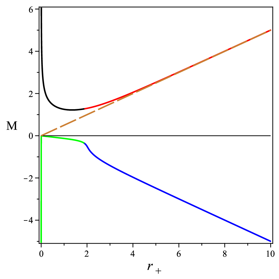
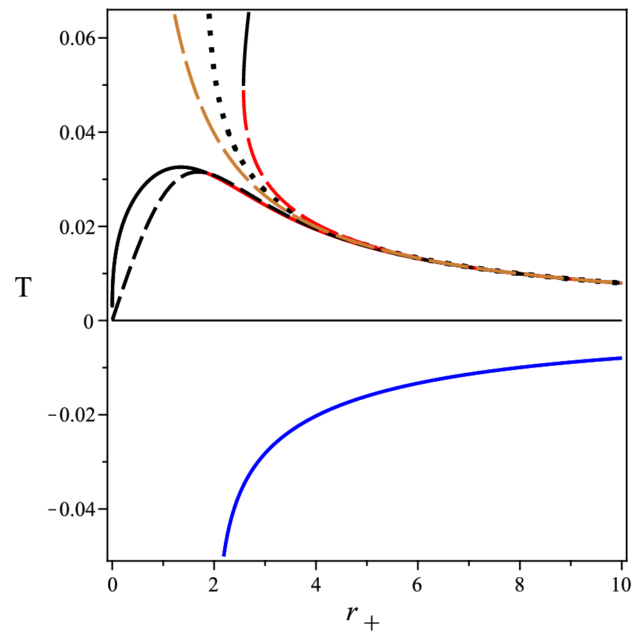
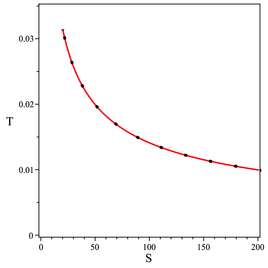
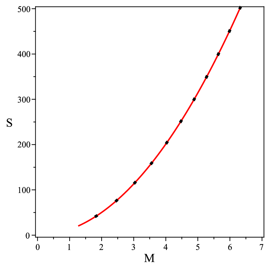
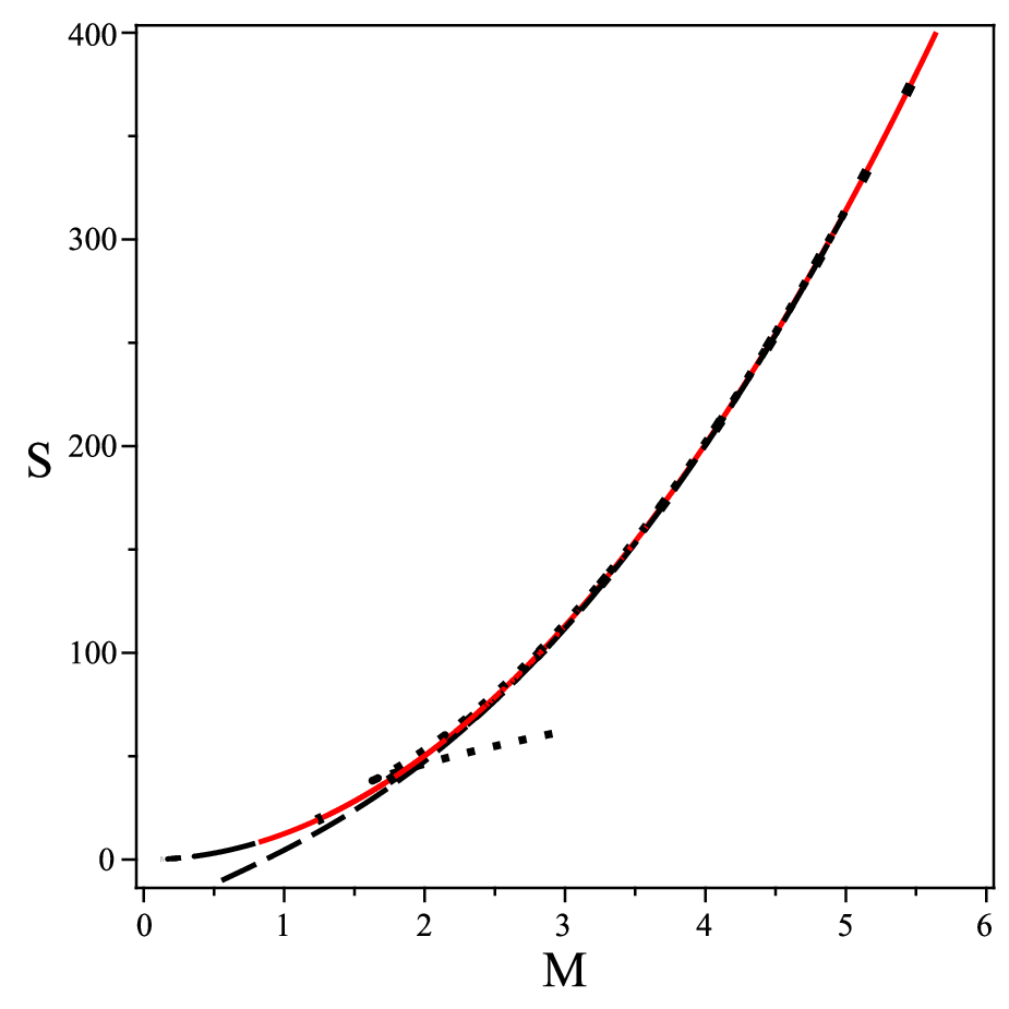
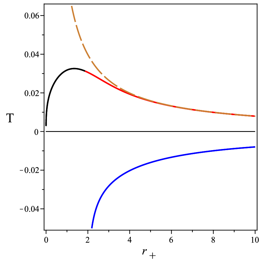
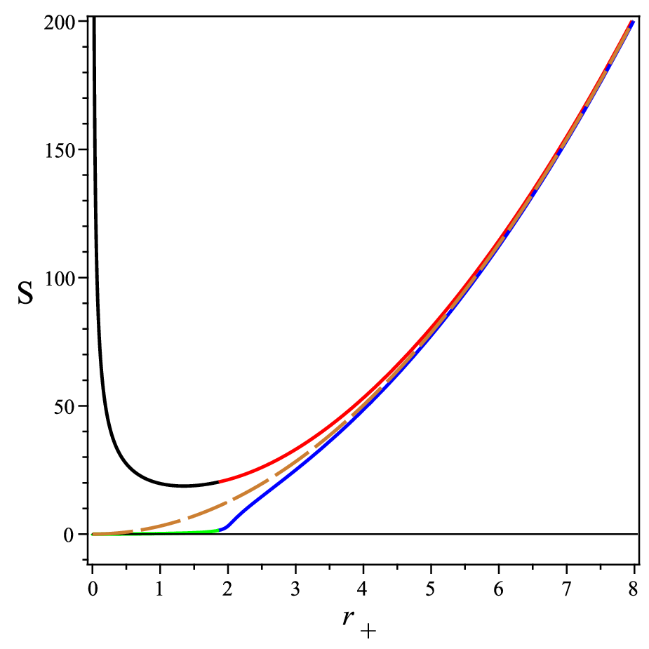
Inserting (32)-(2) into the thermodynamical quantities and plotting them, one can arrive Figs. 1, 3 and 5. In Fig. 1, we have illustrated the temperature, entropy, and mass for different values of parameters. In these figures, the black and red solid lines correspond to the physical solutions, while the green and blue solid lines correspond to the non-physical black hole solutions. The physical solutions have positive temperatures and mass. In these figures, the behavior of the red solid lines is similar to the Schwarzschild black hole, and the behavior of the black solid lines is different from that of Schwarzschild black holes. In Fig. 1a, we observe that, unlike the Einstein gravity case, it no longer diverges for r+→0r_{+}\to 0. Instead, there is a maximum value Tm​a​xT_{max} that is reached at r+,m​a​xr_{+,max}.

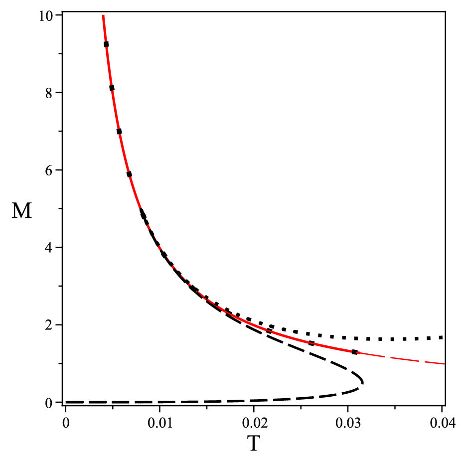
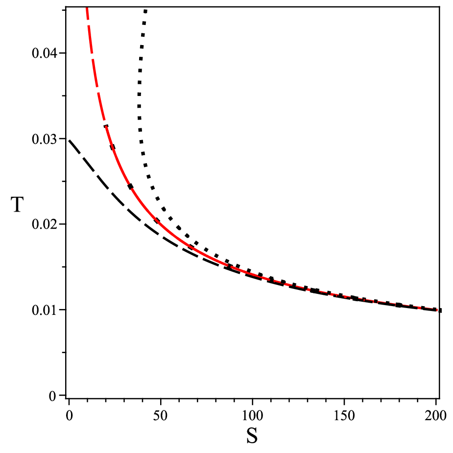
In Fig. 1b, c, the behavior of entropy and mass in the large radii are similar to the Schwarzschild black hole and in the small radii, unlike the Einstein gravity case, diverge for r+→0r_{+}\to 0. Different panels of Fig. 2, compare our black hole solutions (solid and long dashed lines) with those obtained in [17, 18, 19] (dashed and dotted lines). The solid and dashed lines are the results of our calculus and the paper [17, 18, 19] for positive α\alpha, respectively. The long dashed and dotted lines are the results of our calculus and the paper [17, 18, 19] for negative α\alpha, respectively. As can be seen, there is a good agreement in both cases between our computations and the results of the mentioned papers in large radii and somewhat different in small radii but have the same behavior. This shows that the first law of thermodynamic and the Smarr formula in the form of (25) and (26) are valid for this theory of gravity.
Refer to caption
Refer to caption
Refer to caption
Figure 1: The temperature, entropy and mass as a function of r+r_{+} for c1=−0.25,α=0.5c_{1}=-0.25,\alpha=0.5. The orange long dashed lines related to the Schwarzschild’s black hole.
Refer to caption
Refer to caption
Refer to caption
Figure 2: The temperature, entropy and mass as a function of r+r_{+} for c1=−0.25,α=0.5c_{1}=-0.25,\alpha=0.5: solid lines are the results of our method and dashed lines are the results of the paper [17]-[18]. For α=−0.5\alpha=-0.5: Long dashed lines are the results of our method and dotted lines are for the paper [17]-[18]. The orange long dashed lines related to the Schwarzschild’s black hole.

In the following, we are going to look at the thermodynamical stability of the solutions. In global stability, we allow a system in equilibrium with a thermodynamic reservoir to exchange energy with the reservoir. The preferred phase of the system is the one that minimizes the free energy. In order to investigate the global stability, we use the following expression for the free energy

F=M−T​S.F=M-TS. (35)

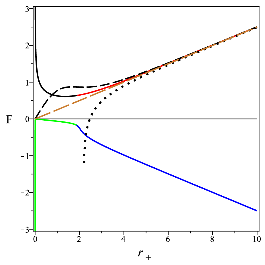
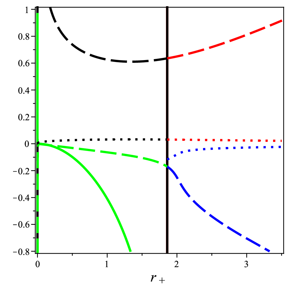
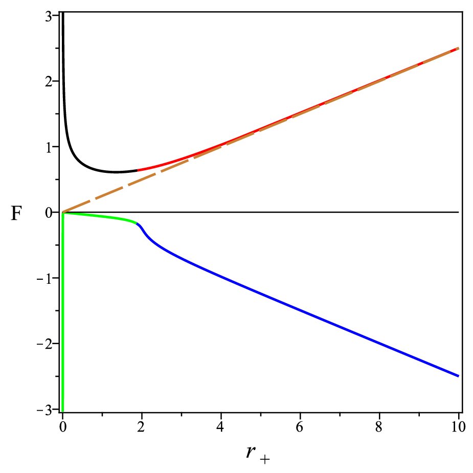
In Fig. 3a, we have shown the free energy in terms of r+r_{+} for positive α\alpha. As can be seen in the black, green, and blue branches the free energy is decreasing functions of r+r_{+}. This shows the black holes in these branches globally are stable. While in the red branch, the free energy has an increasing behavior and is a globally unstable branch.

On the other hand, local stability is concerned with how the system responds to small changes in its thermodynamic parameters. In order to study the thermodynamic stability of the black holes with respect to small variations of the thermodynamic coordinates, one can investigate the behavior of the heat capacity. The positivity of the heat capacity ensures local stability. The heat capacity is given by

C=∂M∂T.C=\dfrac{\partial M}{\partial T}. (36)

In Fig. 3b, heat capacity in terms of r+r_{+} for positive α\alpha have been illustrated. As can be seen the heat capacity in all radii is negative, this shows the black hole in all branches locally unstable.

In Fig. 4, the heat capacity and free energy are compared based on our calculations and the results of papers [17]-[18]. As can be seen from the dashed lines of both figures, the black holes in small radii are locally stable but globally unstable.
Refer to caption
Refer to caption
Figure 3: The free energy and heat capacity as a function of r+r_{+} for c1=−0.25,α=0.5c_{1}=-0.25,\alpha=0.5. The orange long dashed lines related to the Schwarzschild’s black hole.
Refer to caption
Refer to caption
Figure 4: The free energy and heat capacity as a function of r+r_{+} for c1=−0.25,α=0.5c_{1}=-0.25,\alpha=0.5: solid lines are the results of our method and dashed lines are the results of the paper [17]-[18]. For α=−0.5\alpha=-0.5: Long dashed lines are the results of our method and dotted lines are for the paper [17]-[18]. The orange long dashed lines related to the Schwarzschild’s black hole.
Refer to caption
Refer to caption
Refer to caption
Figure 5: The plots of temperature, entropy and mass for c1=−0.25,α=0.5c_{1}=-0.25,\alpha=0.5.
Refer to caption
Refer to caption
Refer to caption
Figure 6: The temperature, entropy and mass as a function of r+r_{+} for c1=−0.25,α=0.5c_{1}=-0.25,\alpha=0.5: solid lines are the results of our method and dashed lines are the results of the paper [17]-[18]. For α=−0.5\alpha=-0.5: Long dashed lines are the results of our method and dotted lines are for the paper [17]-[18].
Figure 7: The temperature (dotted line), heat capacity (solid line) and free energy (dashed line) as a function of r+r_{+} for c1=−0.25,α=0.5c_{1}=-0.25,\alpha=0.5.
Refer to caption

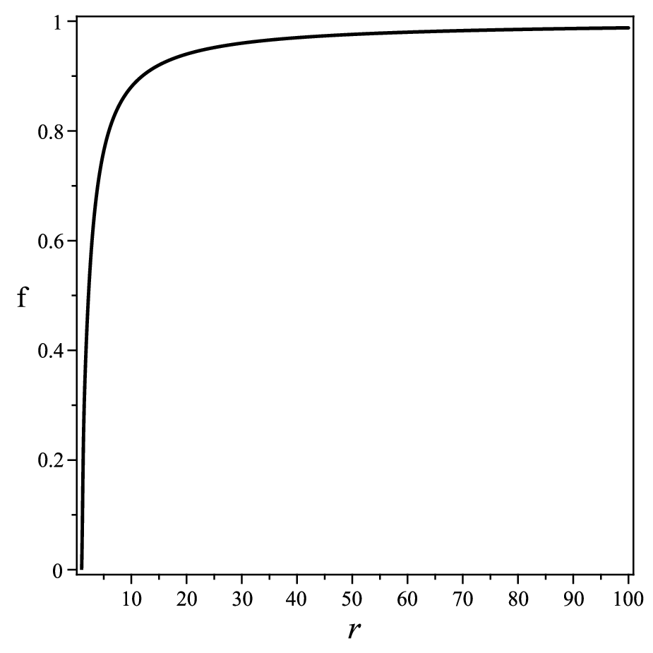
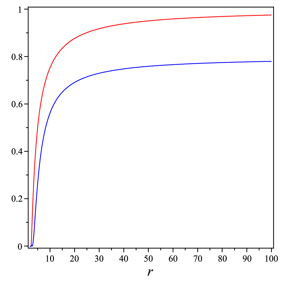
In panels of Fig. 8, we have depicted the metric functions. In Figs. 8a and b, the mass of the black hole is positive and these solutions are similar to Schwarzschild’s black hole. In Figs (8)c and d, the mass of black holes are negative and their behavior is different from the Schwarzschild black hole.

Refer to caption
(a) r+=6.21,M=3.11r_{+}=6.21,M=3.11
Refer to caption
(b) n​e​a​r​h​o​r​i​z​o​nnear\;horizon
Refer to caption
(c) a​s​y​m​p​t​o​t​i​casymptotic
Refer to caption
(d) r+=1.0,M=1.28r_{+}=1.0,M=1.28
Refer to caption
(e) n​e​a​r​h​o​r​i​z​o​nnear\;horizon
Refer to caption
(f) a​s​y​m​p​t​o​t​i​casymptotic
Refer to caption
(g) r+=1.0,M=−0.11r_{+}=1.0,M=-0.11
Refer to caption
(h) n​e​a​r​h​o​r​i​z​o​nnear\;horizon
Refer to caption
(i) a​s​y​m​p​t​o​t​i​casymptotic
Figure 8: The plots of metric for c1=−0.25,α=0.5c_{1}=-0.25,\alpha=0.5.

3 New Solutions

Here, in order to obtain the new static, spherically symmetric black hole solutions of theory we consider a line element with different metric functions. We consider the following static metric

d​s2=−h⁡(r)​d​t2+d​r2f⁡(r)+r2​(d​θ2+sin2⁡(θ)​d​ϕ2).ds^{2}=-h(r)dt^{2}+\dfrac{dr^{2}}{f(r)}+r^{2}\left(d\theta^{2}+\sin^{2}(\theta)d\phi^{2}\right). (37)

Unlike the previous section, here we have two metric functions that require two components of field equations to obtain them. By inserting the metric into the field equations, the differential equations for f⁡(r)f(r) and h⁡(r)h(r) become

8​r4​h4​Err\displaystyle 8r^{4}h^{4}E^{r}_{r} =h3​r4​f′​h′+4​h4​r3​f′+8​r2​f​h4+8​r3​h3​f​h′+2​r4​f​h3​h′′−h2​r4​f​h′2−8​r2​h4−\displaystyle=h^{3}r^{4}f^{\prime}h^{\prime}+4h^{4}r^{3}f^{\prime}+8r^{2}fh^{4}+8r^{3}h^{3}fh^{\prime}+2r^{4}fh^{3}h^{\prime\prime}-h^{2}r^{4}fh^{\prime 2}-8r^{2}h^{4}-
α[−12r2h3h′f′3−48rfh3f′h′′+24rhf2h′3−24rh3h′f′2−48rf2h2h′h′′+\displaystyle\alpha[-12r^{2}h^{3}h^{\prime}f^{\prime 3}-48rfh^{3}f^{\prime}h^{\prime\prime}+24rhf^{2}h^{\prime 3}-24rh^{3}h^{\prime}f^{\prime 2}-48rf^{2}h^{2}h^{\prime}h^{\prime\prime}+
24​r​f2​h2​f′​h′2+24​f​r2​h2​h′2​f′2−24​r​h​f3​h′3−24​r2​f​h3​f′2​h′′−48​f2​h3​h′​f′\displaystyle 24rf^{2}h^{2}f^{\prime}h^{\prime 2}+24fr^{2}h^{2}h^{\prime 2}f^{\prime 2}-24rhf^{3}h^{\prime 3}-24r^{2}fh^{3}f^{\prime 2}h^{\prime\prime}-48f^{2}h^{3}h^{\prime}f^{\prime}
+48​r​f2​h3​f′​h′′+48​r​f3​h2​h′​h′′+12​r2​f3​h′4+48​f​h3​h′​f′+24​r2​f2​h2​f′​h′​h′′\displaystyle+48rf^{2}h^{3}f^{\prime}h^{\prime\prime}+48rf^{3}h^{2}h^{\prime}h^{\prime\prime}+12r^{2}f^{3}h^{\prime 4}+48fh^{3}h^{\prime}f^{\prime}+24r^{2}f^{2}h^{2}f^{\prime}h^{\prime}h^{\prime\prime}
+48rfh3h′f′2−24r2hf2f′h′3−24r2f3hh′2h′′],\displaystyle+48rfh^{3}h^{\prime}f^{\prime 2}-24r^{2}hf^{2}f^{\prime}h^{\prime 3}-24r^{2}f^{3}hh^{\prime 2}h^{\prime\prime}], (38)

and

−4​r4​h4​Eaa\displaystyle-4r^{4}h^{4}E^{a}_{a} =−3​r4​h3​f′​h′−6​r4​h3​f​h′′−12​r3​h4​f′−12​r2​f​h4−12​f​r3​h3​h′+3​r4​f​h2​h′2+12​r2​h4\displaystyle=-3r^{4}h^{3}f^{\prime}h^{\prime}-6r^{4}h^{3}fh^{\prime\prime}-12r^{3}h^{4}f^{\prime}-12r^{2}fh^{4}-12fr^{3}h^{3}h^{\prime}+3r^{4}fh^{2}h^{\prime 2}+12r^{2}h^{4}
+3α[−16r2fh3f′2h′′+32rf2h3f′h′′+32rfh3h′f′2−16r2hf2f′h′3−16r2hf3h′′h′2\displaystyle+3\alpha[-16r^{2}fh^{3}f^{\prime 2}h^{\prime\prime}+32rf^{2}h^{3}f^{\prime}h^{\prime\prime}+32rfh^{3}h^{\prime}f^{\prime 2}-16r^{2}hf^{2}f^{\prime}h^{\prime 3}-16r^{2}hf^{3}h^{\prime\prime}h^{\prime 2}
+16​r​f2​h2​f′​h′2+16​r2​f2​h2​f′​h′​h′′+16​r2​f​h2​f′2​h′2−8​r2​h3​h′​f′3+8​r2​f3​h′4−16​r​h​f3​h′3\displaystyle+16rf^{2}h^{2}f^{\prime}h^{\prime 2}+16r^{2}f^{2}h^{2}f^{\prime}h^{\prime}h^{\prime\prime}+16r^{2}fh^{2}f^{\prime 2}h^{\prime 2}-8r^{2}h^{3}h^{\prime}f^{\prime 3}+8r^{2}f^{3}h^{\prime 4}-16rhf^{3}h^{\prime 3}
+32​r​h2​f3​h′​h′′−32​f2​h3​h′​f′−32​r​f2​h2​h′​h′′−32​r​f​h3​f′​h′′+16​r​h​f2​h′3−16​r​h3​f′2​h′\displaystyle+32rh^{2}f^{3}h^{\prime}h^{\prime\prime}-32f^{2}h^{3}h^{\prime}f^{\prime}-32rf^{2}h^{2}h^{\prime}h^{\prime\prime}-32rfh^{3}f^{\prime}h^{\prime\prime}+16rhf^{2}h^{\prime 3}-16rh^{3}f^{\prime 2}h^{\prime}
+32fh3h′f′].\displaystyle+32fh^{3}h^{\prime}f^{\prime}]. (39)

Similar to the previous section, expanding the function h⁡(r)h(r) and f⁡(r)f(r) around the event horizon r+r_{+}

f⁡(r)\displaystyle f(r) =f1​(r−r+)+f2​(r−r+)2+f3​(r−r+)3+…\displaystyle=f_{1}(r-r_{+})+f_{2}(r-r_{+})^{2}+f_{3}(r-r_{+})^{3}+... (40)
h⁡(r)\displaystyle h(r) =h1​(r−r+)+h2​(r−r+)2+h3​(r−r+)3+…\displaystyle=h_{1}(r-r_{+})+h_{2}(r-r_{+})^{2}+h_{3}(r-r_{+})^{3}+... (41)

and then inserting these expressions into the field equations, we find

f2=h1​r+2−h1​f1​r+3+6​α​f13​h2​r+2+6​α​h1​f12+12​α​r+​h2​f126​α​r+​f1​h1​(2+r+​f1),\displaystyle f_{2}={\dfrac{h_{1}r_{+}^{2}-h_{1}f_{1}r_{+}^{3}+6\alpha f_{1}^{3}h_{2}r_{+}^{2}+6\alpha h_{1}f_{1}^{2}+12\alpha r_{+}h_{2}f_{1}^{2}}{6\alpha r_{+}f_{1}h_{1}(2+r_{+}f_{1})},} (42)

where r+r_{+}, f1f_{1}, h1h_{1} and h2h_{2} are undetermined constants of integration. The other near horizon constants provided in the Appendixes B. In the large rr limit, we linearize the field equations near the Schwarzschild background

f⁡(r)\displaystyle f(r) =1−2​Mr+ϵ​F​(r),\displaystyle=1-\dfrac{2M}{r}+\epsilon F(r), (43)
h⁡(r)\displaystyle h(r) =1−2​Mr+ϵ​H​(r),\displaystyle=1-\dfrac{2M}{r}+\epsilon H(r), (44)

where F⁡(r)F(r) and H⁡(r)H(r) are determined by the field equations, and we linearize the differential equations by keeping terms only to order ϵ\epsilon. The resulting differential equations for F⁡(r)F(r) and H⁡(r)H(r) take the form

H′′+γ⁡(r)​H′+η⁡(r)​F′+ω⁡(r)​F​(r)+Ξ⁡(r)​H​(r)+g⁡(r)\displaystyle H^{\prime\prime}+\gamma(r)H^{\prime}+\eta(r)F^{\prime}+\omega(r)F(r)+\Xi(r)H(r)+g(r) =0,\displaystyle=0, (45)
H′′+γ¯​(r)​H′+η¯​(r)​F′+ω¯​(r)​F​(r)+Ξ¯​(r)​H​(r)+g¯​(r)\displaystyle H^{\prime\prime}+\bar{\gamma}(r)H^{\prime}+\bar{\eta}(r)F^{\prime}+\bar{\omega}(r)F(r)+\bar{\Xi}(r)H(r)+\bar{g}(r) =0,\displaystyle=0, (46)

where the functions shown in the above equations are given in the appendix C. In the large rr limit, the homogenous equations read

H′′+4r​H′+2r​F′+4​Fr2−4​M​Hr3\displaystyle H^{\prime\prime}+\dfrac{4}{r}H^{\prime}+\dfrac{2}{r}F^{\prime}+\dfrac{4F}{r^{2}}-\dfrac{4MH}{r^{3}} =0,\displaystyle=0, (47)
H′′+2r​H′+2r​F′+2​Fr2+2​M2​Hr4\displaystyle H^{\prime\prime}+\dfrac{2}{r}H^{\prime}+\dfrac{2}{r}F^{\prime}+\dfrac{2F}{r^{2}}+\dfrac{2M^{2}H}{r^{4}} =0.\displaystyle=0. (48)

Equations (47) and (48) can be solved exactly to obtain

F⁡(r)\displaystyle F(r) =Mπ​r2​[2​c2′​r​e−(M+2​r)2r2+π​(M+2​r)​(c1′+c2′​𝑒𝑟𝑓​(2+Mr))],\displaystyle=\dfrac{M}{\sqrt{\pi}r^{2}}\left[2c_{2}^{\prime}re^{-\dfrac{(M+2r)^{2}}{r^{2}}}+\sqrt{\pi}(M+2r)\left(c_{1}^{\prime}+c_{2}^{\prime}{\it erf}\left(2+\dfrac{M}{r}\right)\right)\right], (49)
H⁡(r)\displaystyle H(r) =c1+c2​𝑒𝑟𝑓​(2+Mr).\displaystyle=c_{1}+c_{2}{\it erf}\left(2+\dfrac{M}{r}\right). (50)

In the large rr, F⁡(r)F(r) and H⁡(r)H(r) become

F⁡(r)≈\displaystyle F(r)\approx 2​M​(π​c1′+π​c2′​𝑒𝑟𝑓​(2)+c2′​e−4)π​r+M2​(π​c1′+π​c2′​𝑒𝑟𝑓​(2)−c2′​e−4)π​r2+8​c2′​e−4​M3π​r3\displaystyle\dfrac{2M(\sqrt{\pi}c_{1}^{\prime}+\sqrt{\pi}c_{2}^{\prime}{\it erf}(2)+c_{2}^{\prime}e^{-4})}{\sqrt{\pi}r}+\dfrac{M^{2}(\sqrt{\pi}c_{1}^{\prime}+\sqrt{\pi}c_{2}^{\prime}{\it erf}(2)-c_{2}^{\prime}e^{-4})}{\sqrt{\pi}r^{2}}+\dfrac{8c_{2}^{\prime}e^{-4}M^{3}}{\sqrt{\pi}r^{3}}
−8​c2′​e−4​M4π​r4+𝒪⁡(r−5),\displaystyle-\dfrac{8c_{2}^{\prime}e^{-4}M^{4}}{\sqrt{\pi}r^{4}}+\mathcal{O}(r^{-5}), (51)
H⁡(r)≈\displaystyle H(r)\approx c1+c2​𝑒𝑟𝑓​(2)+2​c2​e−4​Mπ​r−4​c2​e−4​M2π​r2+14​c2​e−4​M33​π​r3−10​c2​e−4​M43​π​r4+𝒪⁡(r−5).\displaystyle c_{1}+c_{2}{\it erf}(2)+\dfrac{2c_{2}e^{-4}M}{\sqrt{\pi}r}-\dfrac{4c_{2}e^{-4}M^{2}}{\sqrt{\pi}r^{2}}+\dfrac{14c_{2}e^{-4}M^{3}}{3\sqrt{\pi}r^{3}}-\dfrac{10c_{2}e^{-4}M^{4}}{3\sqrt{\pi}r^{4}}+\mathcal{O}(r^{-5}). (52)

As we know, for α→0\alpha\to 0, the metric is expected to return to the Schwarzschild metric. To fulfill this desire, we must have: c1=c1′=c2=c2′=0c_{1}=c_{1}^{\prime}=c_{2}=c_{2}^{\prime}=0. To obtain the particular solution, we consider the following expansions

fp​(r)=\displaystyle f_{p}(r)= ∑n=2Fnrn=F2r2+F3r3​…\displaystyle\sum_{n=2}\dfrac{F_{n}}{r^{n}}=\dfrac{F_{2}}{r^{2}}+\dfrac{F_{3}}{r^{3}}... (53)
hp​(r)=\displaystyle h_{p}(r)= ∑n=2Hnrn=H2r2+H3r3​…\displaystyle\sum_{n=2}\dfrac{H_{n}}{r^{n}}=\dfrac{H_{2}}{r^{2}}+\dfrac{H_{3}}{r^{3}}... (54)

Inserting the above expansions into the field equations and solving order by order, one can get

fp​(r)\displaystyle f_{p}(r) =−1120​α​M33​r7−288​α​M4r8−756​α​M5r9−2016​α​M6r10−27216​α​M75​r11+𝒪⁡(1r12)\displaystyle=-\dfrac{1120\alpha M^{3}}{3r^{7}}-\dfrac{288\alpha M^{4}}{r^{8}}-\dfrac{756\alpha M^{5}}{r^{9}}-\dfrac{2016\alpha M^{6}}{r^{10}}-\dfrac{27216\alpha M^{7}}{5r^{11}}+\mathcal{O}\left(\dfrac{1}{r^{12}}\right) (55)
hp​(r)\displaystyle h_{p}(r) =−256​α​M33​r7−108​α​M4r8−252​α​M5r9−3024​α​M65​r10−81648​α​M755​r11+𝒪⁡(1r12).\displaystyle=-\dfrac{256\alpha M^{3}}{3r^{7}}-\dfrac{108\alpha M^{4}}{r^{8}}-\dfrac{252\alpha M^{5}}{r^{9}}-\dfrac{3024\alpha M^{6}}{5r^{10}}-\dfrac{81648\alpha M^{7}}{55r^{11}}+\mathcal{O}\left(\dfrac{1}{r^{12}}\right). (56)

In large rr, the solutions are:

f⁡(r)≈1−2​Mr+fp,h⁡(r)≈1−2​Mr+hp.f(r)\approx 1-\dfrac{2M}{r}+f_{p},\;\;\;\;\;h(r)\approx 1-\dfrac{2M}{r}+h_{p}. (57)

We wish to obtain an approximate analytic solution that is valid near the horizon and at large rr. To this end we employ a continued fraction expansion, and write

h⁡(r)=x​A​(x),h⁡(r)f⁡(r)=B2​(x),h(r)=xA(x),\hskip 14.22636pt\dfrac{h(r)}{f(r)}=B^{2}(x), (58)

with

A⁡(x)\displaystyle A(x) =1−ϵ⁡(1−x)+(a0−ϵ)​(1−x)2+A~​(x)​(1−x)3\displaystyle=1-\epsilon(1-x)+(a_{0}-\epsilon)(1-x)^{2}+\tilde{A}(x)(1-x)^{3} (59)
B⁡(x)\displaystyle B(x) =1+b0​(1−x)+B~​(x)​(1−x)2\displaystyle=1+b_{0}(1-x)+\tilde{B}(x)(1-x)^{2} (60)

where

x=1−r+rA~​(x)=a11+a2​x1+a3​x1+a4​x1+…B~​(x)=b11+b2​x1+b3​x1+b4​x1+…x=1-\frac{r_{+}}{r}\qquad\tilde{A}(x)=\dfrac{a_{1}}{1+\dfrac{a_{2}x}{1+\dfrac{a_{3}x}{1+\dfrac{a_{4}x}{1+...}}}}\qquad\tilde{B}(x)=\dfrac{b_{1}}{1+\dfrac{b_{2}x}{1+\dfrac{b_{3}x}{1+\dfrac{b_{4}x}{1+...}}}} (61)

where we truncate the continued fraction at order 44. By expanding (58) near the horizon (x→0x\to 0) and the asymptotic region (x→1x\to 1) we obtain

ϵ=−H1r+−1,b0=F​1−H​12​r+,a0=H2r+2\epsilon=-\dfrac{H_{1}}{r_{+}}-1,\qquad b_{0}=\dfrac{F1-H1}{2r_{+}},\qquad a_{0}=\dfrac{H_{2}}{r_{+}^{2}} (62)

for the lowest order expansion coefficients, with the remaining aia_{i} and bib_{i} given in terms of (r+,h1,f1,h2)(r_{+},h_{1},f_{1},h_{2}); we provide these expressions in the Appendix. For a static space time we have a timelike Killing vector ξ=∂t\xi=\partial_{t} everywhere outside the horizon and so we obtain

T=\displaystyle T= 14​πf⁡(r)h⁡(r)h′(r)|r+=f1​h14​π=(1−2​ϵ+a1+a0)4​π​r+​(1+b1).\displaystyle\dfrac{1}{4\pi}\left.\sqrt{\dfrac{f(r)}{h(r)}}h^{{}^{\prime}}(r)\right|_{r_{+}}=\dfrac{\sqrt{f_{1}h_{1}}}{4\pi}={\dfrac{(1-2\epsilon+a_{1}+a_{0})}{{4\pi r_{+}}\left(1+{b_{1}}\right)}}. (63)

We compute the entropy by using of the first two term in continued fraction expansion as follows [33, 34]

S=\displaystyle S= −2π∫H​o​r​i​z​o​nd2xηδ​Lδ​Ra​b​c​dϵa​bϵc​d=πr+2[1+6α(2​h1r+3−f1​h1r+2+2​h​(r+)​f1f⁡(r+)​r+3+h⁡(r+)​f12f⁡(r+)​r+2+f⁡(r+)​h12h⁡(r+)​r+2)]\displaystyle-2\pi\int_{Horizon}d^{2}x\sqrt{\eta}\dfrac{\delta L}{\delta R_{abcd}}\epsilon_{ab}\epsilon_{cd}=\pi r_{+}^{2}\left[1+6\alpha\left(\dfrac{2h_{1}}{r_{+}^{3}}-\dfrac{f_{1}h_{1}}{r_{+}^{2}}+\dfrac{2h(r_{+})f_{1}}{f(r_{+})r_{+}^{3}}+\dfrac{h(r_{+})f_{1}^{2}}{f(r_{+})r_{+}^{2}}+\dfrac{f(r_{+})h_{1}^{2}}{h(r_{+})r_{+}^{2}}\right)\right]
=π​r+2​[1+6​α​(4​h1r+3+f1​h1r+2)].\displaystyle=\pi r_{+}^{2}\left[1+6\alpha\left(\dfrac{4h_{1}}{r_{+}^{3}}+\dfrac{f_{1}h_{1}}{r_{+}^{2}}\right)\right]. (64)

Then the mass from (25), becomes

M=f1​h1​r+22​[1+6​α​(4​h1r+3+f1​h1r+2)].M=\dfrac{\sqrt{f_{1}h_{1}}r_{+}^{2}}{2}\left[1+6\alpha\left(\dfrac{4h_{1}}{r_{+}^{3}}+\dfrac{f_{1}h_{1}}{r_{+}^{2}}\right)\right]. (65)

To obtain the new black hole solutions we consider the different relations between f1f_{1} and h1h_{1} [35]. In the case of f1=h1f_{1}=h_{1}, we obtain the results of the first section.

3.1 The case h1=f13h_{1}=f_{1}^{3}

We now consider following relation between f1f_{1} and h1h_{1} as

h1​(r+)=f13​(r+).h_{1}(r_{+})=f_{1}^{3}(r_{+}). (66)

From equations (25) and (26), we have

M=f122​r+​(r+3+12​α​r+​f14​(r+)+48​α​f13​(r+)),\displaystyle M=\dfrac{f_{1}^{2}}{2r_{+}}(r_{+}^{3}+12\alpha r_{+}f_{1}^{4}(r_{+})+48\alpha f_{1}^{3}(r_{+})), (67)
2​r+4​f1′​(r+)+48​α​r+2​f14​(r+)​f1′​(r+)+168​α​r+​f13​(r+)​f1′​(r+)+f1​(r+)​r+3−24​α​f14​(r+)=0.\displaystyle 2r_{+}^{4}f_{1}^{\prime}(r_{+})+48\alpha r_{+}^{2}f_{1}^{4}(r_{+})f_{1}^{\prime}(r_{+})+168\alpha r_{+}f_{1}^{3}(r_{+})f^{\prime}_{1}(r_{+})+f_{1}(r_{+})r_{+}^{3}-24\alpha f_{1}^{4}(r_{+})=0. (68)

Solving (68), one can achieve following equation as

12​r+2​f14+24​α​f17r++6​α​f18+c1=0\dfrac{1}{2}r_{+}^{2}f_{1}^{4}+\dfrac{24\alpha f_{1}^{7}}{r_{+}}+6\alpha f_{1}^{8}+c_{1}=0 (69)

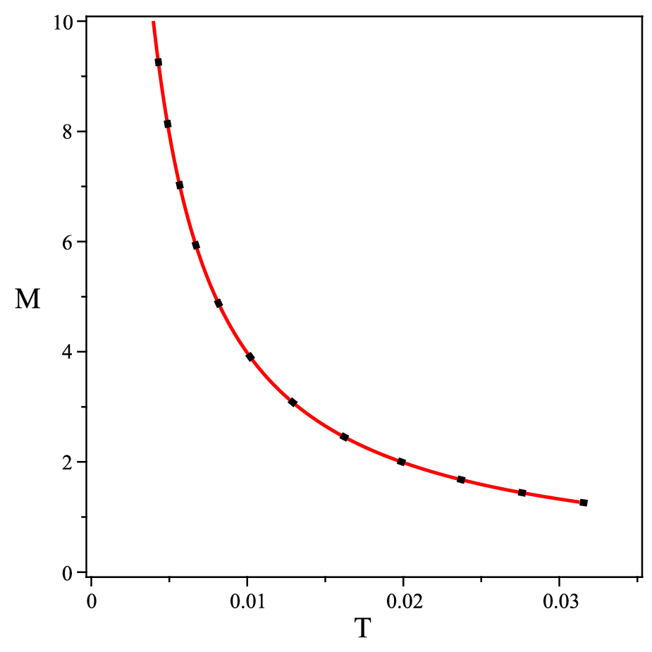
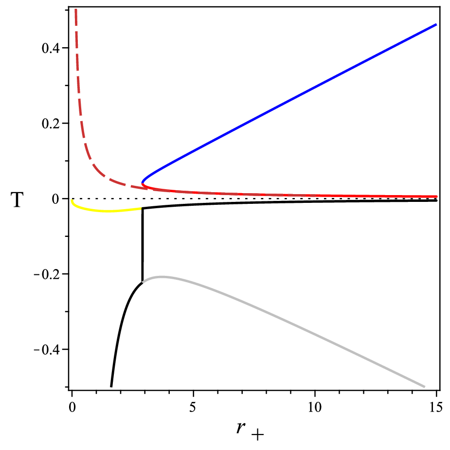
which leads to a maximum of eight solutions for f1​(r+)f_{1}(r_{+}) depending on the value of parameters. Inserting the solutions of (69) into the thermodynamical quantities, one can obtain the analytical solutions for them, which we have plotted in Figs. 9 and 10. In these figures, the dashed orange lines are the behavior of the thermodynamical quantities of Schwarzschild’s black hole. In Fig. (9), the blue and red solid lines are the physical branches, because the temperatures and the mass of these branches are positive. Also, the red branch is globally and locally unstable and the blue branch is globally stable while locally unstable (Fig. (10)). From the Fig. (11), there is a divergence in the heat capacity, but this divergence does not coincide with the extremum points of temperature and free energy. So, the phase transition does not occur.
Refer to caption
Refer to caption
Refer to caption
Figure 9: The temperature, entropy and mass as a function of r+r_{+} for c1=α=−0.5c_{1}=\alpha=-0.5. The orange dashed lines related to the Schwarzschild’s black hole.
Refer to caption
Refer to caption
Figure 10: The free energy and heat capacity as a function of r+r_{+} for c1=α=−0.5c_{1}=\alpha=-0.5. The orange dashed lines related to the Schwarzschild’s black hole.
Figure 11: The temperature (dotted line), heat capacity (solid line) and free energy (dashed line) as a function of r+r_{+} for c1=−0.25,α=−0.5c_{1}=-0.25,\alpha=-0.5.
Refer to caption

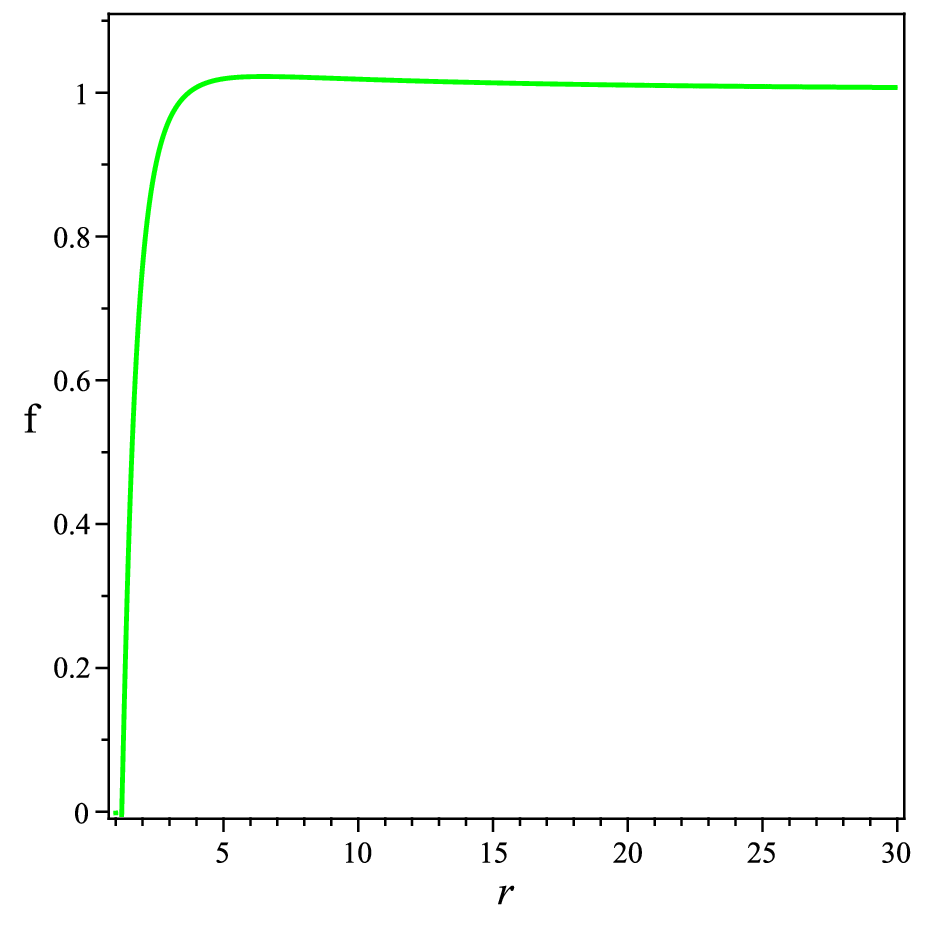
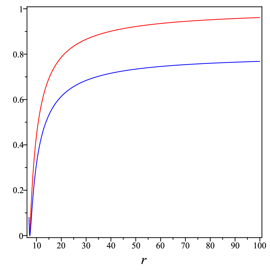
In panels of Fig. 12, we have depicted the metric functions. In these figures, the mass of the black hole is positive and these solutions are similar to Schwarzschild’s black hole.
Refer to caption
(a) h2=1,r+=6h_{2}=1,r_{+}=6
Refer to caption
(b) h2=2,r+=6h_{2}=2,r_{+}=6
Refer to caption
(c) h2=1,r+=2h_{2}=1,r_{+}=2
Figure 12: The behavior of f⁡(r)f(r) (blue line) and 0.8​h​(r)0.8h(r) (red line) in terms of rr for c1=α=−0.5c_{1}=\alpha=-0.5. Left: correspond to the red branch. Middle: correspond to the blue branch. Right: correspond to the yellow branch in figures 9.

4 Conclusion

In this paper, we studied the black hole solutions of Einsteinian cubic gravities by using continued fraction approximations. To get a complete solution, first, we constructed the near horizon and then asymptotic solutions and then used them to obtain an approximate analytic solution using a continued-fraction expansion. Then, we calculated the thermodynamic quantities like entropy, temperature and mass, and by inserting them in the first law and Smarr formula, we obtained the analytic solutions for the near horizon quantities. Then, one can obtain a metric according to continued fraction expansion that is only a function of constant integration not extra function like f1f_{1} or h1h_{1}. We also showed that continued fraction expansion can be used to accurately approximate black hole solutions in cubic gravity, which are valid everywhere outside of the event horizon. Finally, to obtain the new black hole solutions, we considered the different relationships between the near horizon constants. We also compared our results with those of previous works on the subject and we found a good agreement between them.
The important point in our work is that we assumed the near horizon constant f1f_{1} in the first law of thermodynamic and the Smarr formula, is a function of the event horizon radius. This assumption is correct, because f1f_{1} is proportional to temperature according to Equation (23). This method is different from the one used in previous papers like [17]-[18]. First, they used the differential equations for metric function which have been obtained from the action of the theory, while, we have used the components of the field equations (2) of the theory. Second, they obtained the thermodynamical quantities from the first and the second term of near horizon expansion, while we obtained from the first law of thermodynamics and Smarr formula. Our method is applicable to every theory of gravity (as we previously applied to the quadratic gravity in reference [32]), while the method of the papers is only applicable for the theory in which the on-shell action is integrable with respect to rr. Finally, this approach also allows us to obtain black hole solutions different from Einstein gravity solutions by assuming f1≠h1f_{1}\neq h_{1} in the near horizon expansion as we have done in section (3). We think using the thermodynamics to obtain the black hole solutions is a normal approach with respect to one in the references [17]-[18].

We leave for future work, obtaining the non-vacuum, rotating black hole, and other solutions of the theory by using the continued fraction expansion.

Acknowledgements

We thank the support of Iran National Science Foundation 99022223.

Appendix A Explicit Terms in the Continued Fraction Approximation

We present terms up to fourth order in the continued fraction approximation:

ϵ=−F1r+−1,a1=−1−a0+2​ϵ+r+​f1,a2=−4​a1−5​ϵ+1+3​a0+f2​r+2a1\displaystyle\epsilon=-\dfrac{F_{1}}{r_{+}}-1,\,\,\,\,a_{1}=-1-a_{0}+2\epsilon+r_{+}f_{1},\,\,\,\,a_{2}=-{\dfrac{4a_{1}-5\epsilon+1+3a_{0}+f_{2}r_{+}^{2}}{{a_{1}}}}
a3=−1a1​a2​[−f3​r+3+a1​a22+5​a1​a2+6​a0+10​a1−9​ϵ+1]\displaystyle a_{3}=-\dfrac{1}{{a_{1}}{a_{2}}}[-{f_{3}}{{r_{+}}}^{3}+{a_{1}}{{a_{2}}}^{2}+5{a_{1}}{a_{2}}+6{a_{0}}+10{a_{1}}-9\epsilon+1] (70)
a4=−f4​r+4+a1​a23+2​a1​a22​a3+a1​a2​a32+6​a1​a22+6​a1​a2​a3+15​a1​a2+10​a0+20​a1−14​ϵ+1a1​a2​a3\displaystyle a_{4}=-\dfrac{{f_{4}}{{r_{+}}}^{4}+{a_{1}}{{a_{2}}}^{3}+2{a_{1}}{{a_{2}}}^{2}{a_{3}}+{a_{1}}{a_{2}}{{a_{3}}}^{2}+6{a_{1}}{{a_{2}}}^{2}+6{a_{1}}{a_{2}}{a_{3}}+15{a_{1}}{a_{2}}+10{a_{0}}+20{a_{1}}-14\epsilon+1}{{a_{1}}{a_{2}}{a_{3}}}

Appendix B Near Horizon Constants

Here, we present some near horizon constants regarding section (2) and (3) as follows:
The quantity f4f_{4} is given in (2)

f4\displaystyle f_{4} =−13​[r+10​(r+3+48​α​f1+24​r+​α​f12)​(48​r+​α​f12+96​α​f1+r+3)][−31r+12+7524r+10f12α\displaystyle=\dfrac{-1}{3[{{r_{+}}^{10}({r_{+}}^{3}+48\,\alpha\,f_{1}+24\,{r_{+}}\,\alpha\,{f_{{1}}}^{2})(48\,{r_{+}}\,\alpha\,{f_{1}}^{2}+96\,\alpha\,f_{1}+{r_{+}}^{3})}]}[-31\,{r_{+}}^{12}+7524\,{r_{+}}^{10}{f_{1}}^{2}\alpha
−11064​r+11​f13​α−4608​r+6​α2​f12−86400​r+4​α3​f14+10944​r+7​f13​α2−1534464​r+2​α4​f16+\displaystyle-11064\,{r_{+}}^{11}{f_{1}}^{3}\alpha-4608\,{r_{+}}^{6}{\alpha}^{2}{f_{1}}^{2}-86400\,{r_{+}}^{4}{\alpha}^{3}{f_{1}}^{4}+10944\,{r_{+}}^{7}{f_{1}}^{3}{\alpha}^{2}-1534464\,{r_{+}}^{2}{\alpha}^{4}{f_{1}}^{6}+
888192​r+5​α3​f15−89136​r+8​f14​α2−5971968​α5​f18+5640192​α4​f17​r+3−1769472​α3​f16​r+6+\displaystyle 888192\,{r_{+}}^{5}{\alpha}^{3}{f_{1}}^{5}-89136\,{r_{+}}^{8}{f_{1}}^{4}{\alpha}^{2}-5971968\,{\alpha}^{5}{f_{1}}^{8}+5640192\,{\alpha}^{4}{f_{1}}^{7}{r_{+}}^{3}-1769472\,{\alpha}^{3}{f_{1}}^{6}{r_{+}}^{6}+
184896r+9f15α2+1248αr+9f1+34r+13f1−864αr+8].\displaystyle 184896\,{r_{+}}^{9}{f_{1}}^{5}{\alpha}^{2}+1248\,\alpha\,{r_{+}}^{9}f_{1}+34\,{r_{+}}^{13}f_{1}-864\,\alpha\,{r_{+}}^{8}]. (71)

The near horizon constants regarding section (3):

f3=−12592​(f13​h12​r+2​α2​(r+3​f13+8+6​r+2​f12+12​r+​f1))[6912α2f16h22r+4+71h12r+7f13−\displaystyle f_{3}=-\frac{1}{2592({{f_{{1}}}^{3}{h_{{1}}}^{2}{{\it r_{+}}}^{2}{\alpha}^{2}\left({{\it r_{+}}}^{3}{f_{{1}}}^{3}+8+6\,{{\it r_{+}}}^{2}{f_{{1}}}^{2}+12\,{\it r_{+}}\,f_{{1}}\right)})}[6912{\alpha}^{2}{f_{{1}}}^{6}{h_{{2}}}^{2}{{\it r_{+}}}^{4}+71\,{h_{{1}}}^{2}{{\it r_{+}}}^{7}{f_{{1}}}^{3}-
160​r+6​h12​f12+59​r+5​h12​f1+30​r+4​h12+5472​α2​f16​h12​r+2+4536​α2​f14​h12+8892​α2​f15​h12​r++\displaystyle 160\,{{\it r_{+}}}^{6}{h_{{1}}}^{2}{f_{{1}}}^{2}+59\,{{\it r_{+}}}^{5}{h_{{1}}}^{2}f_{{1}}+30\,{{\it r_{+}}}^{4}{h_{{1}}}^{2}+5472\,{\alpha}^{2}{f_{{1}}}^{6}{h_{{1}}}^{2}{{\it r_{+}}}^{2}+4536\,{\alpha}^{2}{f_{{1}}}^{4}{h_{{1}}}^{2}+8892\,{\alpha}^{2}{f_{{1}}}^{5}{h_{{1}}}^{2}{\it r_{+}}+
876​f14​h12​r+4​α+816​f15​h12​r+5​α−792​r+2​h12​α​f12+1728​α2​f17​h12​r+3+6912​α2​f15​h22​r+3−\displaystyle 876\,{f_{{1}}}^{4}{h_{{1}}}^{2}{{\it r_{+}}}^{4}\alpha+816\,{f_{{1}}}^{5}{h_{{1}}}^{2}{{\it r_{+}}}^{5}\alpha-792\,{{\it r_{+}}}^{2}{h_{{1}}}^{2}\alpha\,{f_{{1}}}^{2}+1728\,{\alpha}^{2}{f_{{1}}}^{7}{h_{{1}}}^{2}{{\it r_{+}}}^{3}+6912\,{\alpha}^{2}{f_{{1}}}^{5}{h_{{2}}}^{2}{{\it r_{+}}}^{3}-
816​h1​r+5​h2​f14​α+1728​α2​f17​h22​r+5+684​f13​h12​r+3​α+576​h1​r+3​h2​f12​α−19584​α2​f15​h1​r+2​h2+\displaystyle 816\,h_{{1}}{{\it r_{+}}}^{5}h_{{2}}{f_{{1}}}^{4}\alpha+1728\,{\alpha}^{2}{f_{{1}}}^{7}{h_{{2}}}^{2}{{\it r_{+}}}^{5}+684\,{f_{{1}}}^{3}{h_{{1}}}^{2}{{\it r_{+}}}^{3}\alpha+576\,h_{{1}}{{\it r_{+}}}^{3}h_{{2}}{f_{{1}}}^{2}\alpha-19584\,{\alpha}^{2}{f_{{1}}}^{5}h_{{1}}{{\it r_{+}}}^{2}h_{{2}}+
2496h1r+4h2f13α−960h1r+6f15αh2−12384α2f16h1r+3h2−3456α2f17h1r+4h2−17280α2f14h2r+h1].\displaystyle 2496\,h_{{1}}{{\it r_{+}}}^{4}h_{{2}}{f_{{1}}}^{3}\alpha-960\,h_{{1}}{{\it r_{+}}}^{6}{f_{{1}}}^{5}\alpha\,h_{{2}}-12384\,{\alpha}^{2}{f_{{1}}}^{6}h_{{1}}{{\it r_{+}}}^{3}h_{{2}}-3456\,{\alpha}^{2}{f_{{1}}}^{7}h_{{1}}{{\it r_{+}}}^{4}h_{{2}}-17280\,{\alpha}^{2}{f_{{1}}}^{4}h_{{2}}{\it r_{+}}\,h_{{1}}]. (72)
h3=−12592​(f14​h1​r+2​α2​(r+3​f13+8+6​r+2​f12+12​r+​f1))[11h12r+7f13−40r+6h12f12+35r+5h12f1\displaystyle h_{3}=-\frac{1}{2592({{f_{{1}}}^{4}h_{{1}}{{\it r_{+}}}^{2}{\alpha}^{2}\left({{\it r_{+}}}^{3}{f_{{1}}}^{3}+8+6\,{{\it r_{+}}}^{2}{f_{{1}}}^{2}+12\,{\it r_{+}}\,f_{{1}}\right)})}[11\,{h_{{1}}}^{2}{{\it r_{+}}}^{7}{f_{{1}}}^{3}-40\,{{\it r_{+}}}^{6}{h_{{1}}}^{2}{f_{{1}}}^{2}+35\,{{\it r_{+}}}^{5}{h_{{1}}}^{2}f_{{1}}
−6​r+4​h12+7200​α2​f16​h12​r+2+8424​α2​f14​h12+12348​α2​f15​h12​r++948​f14​h12​r+4​α+528​f15​h12​r+5​α\displaystyle-6\,{{\it r_{+}}}^{4}{h_{{1}}}^{2}+7200\,{\alpha}^{2}{f_{{1}}}^{6}{h_{{1}}}^{2}{{\it r_{+}}}^{2}+8424\,{\alpha}^{2}{f_{{1}}}^{4}{h_{{1}}}^{2}+12348\,{\alpha}^{2}{f_{{1}}}^{5}{h_{{1}}}^{2}{\it r_{+}}+948\,{f_{{1}}}^{4}{h_{{1}}}^{2}{{\it r_{+}}}^{4}\alpha+528\,{f_{{1}}}^{5}{h_{{1}}}^{2}{{\it r_{+}}}^{5}\alpha
−360​r+2​h12​α​f12+1728​α2​f17​h12​r+3+6912​α2​f15​h22​r+3+6912​α2​f16​h22​r+4+1728​α2​f17​h22​r+5+\displaystyle-360\,{{\it r_{+}}}^{2}{h_{{1}}}^{2}\alpha\,{f_{{1}}}^{2}+1728\,{\alpha}^{2}{f_{{1}}}^{7}{h_{{1}}}^{2}{{\it r_{+}}}^{3}+6912\,{\alpha}^{2}{f_{{1}}}^{5}{h_{{2}}}^{2}{{\it r_{+}}}^{3}+6912\,{\alpha}^{2}{f_{{1}}}^{6}{h_{{2}}}^{2}{{\it r_{+}}}^{4}+1728\,{\alpha}^{2}{f_{{1}}}^{7}{h_{{2}}}^{2}{{\it r_{+}}}^{5}+
252​f13​h12​r+3​α+576​h1​r+3​h2​f12​α−528​h1​r+5​h2​f14​α+1920​h1​r+4​h2​f13​α−672​h1​r+6​f15​α​h2−\displaystyle 252\,{f_{{1}}}^{3}{h_{{1}}}^{2}{{\it r_{+}}}^{3}\alpha+576\,h_{{1}}{{\it r_{+}}}^{3}h_{{2}}{f_{{1}}}^{2}\alpha-528\,h_{{1}}{{\it r_{+}}}^{5}h_{{2}}{f_{{1}}}^{4}\alpha+1920\,h_{{1}}{{\it r_{+}}}^{4}h_{{2}}{f_{{1}}}^{3}\alpha-672\,h_{{1}}{{\it r_{+}}}^{6}{f_{{1}}}^{5}\alpha\,h_{{2}}-
14112α2f16h1r+3h2−23040α2f15h1r+2h2−3456α2f17h1r+4h2−17280α2f14h2r+h1].\displaystyle 14112\,{\alpha}^{2}{f_{{1}}}^{6}h_{{1}}{{\it r_{+}}}^{3}h_{{2}}-23040\,{\alpha}^{2}{f_{{1}}}^{5}h_{{1}}{{\it r_{+}}}^{2}h_{{2}}-3456\,{\alpha}^{2}{f_{{1}}}^{7}h_{{1}}{{\it r_{+}}}^{4}h_{{2}}-17280\,{\alpha}^{2}{f_{{1}}}^{4}h_{{2}}{\it r_{+}}\,h_{{1}}]. (73)
f4=−1248832​(f15​h13​r+3​α3​(r+5​f15+10​r+4​f14+80​r+2​f12+32+40​r+3​f13+80​r+​f1))[−922h13r+7f1\displaystyle f_{4}=\frac{-1}{248832({{f_{{1}}}^{5}{h_{{1}}}^{3}{{r_{+}}}^{3}{\alpha}^{3}\left({{r_{+}}}^{5}{f_{{1}}}^{5}+10\,{{r_{+}}}^{4}{f_{{1}}}^{4}+80\,{{r_{+}}}^{2}{f_{{1}}}^{2}+32+40\,{{r_{+}}}^{3}{f_{{1}}}^{3}+80\,{r_{+}}\,f_{{1}}\right)})}\,[-922\,{h_{{1}}}^{3}{{r_{+}}}^{7}f_{{1}}
+2557​h13​r+11​f15+7713​h13​r+9​f13−8528​h13​r+10​f14−328​h13​r+8​f12+813888​α3​r+3​f18​h2​h12−\displaystyle+2557\,{h_{{1}}}^{3}{r_{+}}^{11}{f_{1}}^{5}+7713\,{h_{1}}^{3}{r_{+}}^{9}{f_{1}}^{3}-8528\,{h_{{1}}}^{3}{{r_{+}}}^{10}{f_{1}}^{4}-328\,{h_{1}}^{3}{r_{+}}^{8}{f_{1}}^{2}+813888\,{\alpha}^{3}{r_{+}}^{3}{f_{1}}^{8}h_{2}{h_{1}}^{2}-
1990656​α3​r+5​f18​h23+8136​f15​h13​r+3​α2−59424​f14​h13​r+6​α−1492992​α3​r+7​f110​h23+\displaystyle 1990656\,{\alpha}^{3}{{r_{+}}}^{5}{f_{1}}^{8}{h_{2}}^{3}+8136\,{f_{1}}^{5}{h_{1}}^{3}{{r_{+}}}^{3}{\alpha}^{2}-59424\,{f_{1}}^{4}{h_{1}}^{3}{{r_{+}}}^{6}\alpha-1492992\,{\alpha}^{3}{{r_{+}}}^{7}{f_{1}}^{10}{h_{2}}^{3}+
247896​f18​h13​r+6​α2+89712​f16​h13​r+4​α2−248832​α3​r+8​f111​h23+143424​f19​h13​r+7​α2+\displaystyle 247896\,{f_{{1}}}^{8}{h_{{1}}}^{3}{{r_{+}}}^{6}{\alpha}^{2}+89712\,{f_{{1}}}^{6}{h_{{1}}}^{3}{{r_{+}}}^{4}{\alpha}^{2}-248832\,{\alpha}^{3}{{r_{+}}}^{8}{f_{{1}}}^{11}{h_{{2}}}^{3}+143424\,{f_{{1}}}^{9}{h_{{1}}}^{3}{{r_{+}}}^{7}{\alpha}^{2}+
384012​f17​h13​r+5​α2+230688​α3​f18​h13​r+2+248832​α3​f110​h13​r+4+316224​α3​f19​h13​r+3+\displaystyle 384012\,{f_{{1}}}^{7}{h_{{1}}}^{3}{{r_{+}}}^{5}{\alpha}^{2}+230688\,{\alpha}^{3}{f_{{1}}}^{8}{h_{{1}}}^{3}{{r_{+}}}^{2}+248832\,{\alpha}^{3}{f_{{1}}}^{10}{h_{{1}}}^{3}{{r_{+}}}^{4}+316224\,{\alpha}^{3}{f_{{1}}}^{9}{h_{{1}}}^{3}{{r_{+}}}^{3}+
654480​α3​f17​h13​r++37164​f17​h13​r+9​α+31788​f13​h13​r+5​α−15924​f16​h13​r+8​α+4824​r+4​h13​α​f12\displaystyle 654480\,{\alpha}^{3}{f_{{1}}}^{7}{h_{{1}}}^{3}{r_{+}}+37164\,{f_{{1}}}^{7}{h_{{1}}}^{3}{{r_{+}}}^{9}\alpha+31788\,{f_{{1}}}^{3}{h_{{1}}}^{3}{{r_{+}}}^{5}\alpha-15924\,{f_{{1}}}^{6}{h_{{1}}}^{3}{{r_{+}}}^{8}\alpha+4824\,{{r_{+}}}^{4}{h_{{1}}}^{3}\alpha\,{f_{{1}}}^{2}
−6480​r+2​h13​α2​f14−7608​h13​r+7​f15​α−2985984​α3​r+6​f19​h23+124416​α3​f111​h13​r+5−\displaystyle-6480\,{{r_{+}}}^{2}{h_{{1}}}^{3}{\alpha}^{2}{f_{{1}}}^{4}-7608\,{h_{{1}}}^{3}{{r_{+}}}^{7}{f_{{1}}}^{5}\alpha-2985984\,{\alpha}^{3}{{r_{+}}}^{6}{f_{{1}}}^{9}{h_{{2}}}^{3}+124416\,{\alpha}^{3}{f_{{1}}}^{11}{h_{{1}}}^{3}{{r_{+}}}^{5}-
288000​α2​r+6​f17​h2​h12−492​r+6​h13+676512​α3​f16​h13+237312​α2​r+9​f19​h22​h1−16128​α​f12​h2​r+5​h12\displaystyle 288000\,{\alpha}^{2}{{r_{+}}}^{6}{f_{{1}}}^{7}h_{{2}}{h_{{1}}}^{2}-492\,{{r_{+}}}^{6}{h_{{1}}}^{3}+676512\,{\alpha}^{3}{f_{{1}}}^{6}{h_{{1}}}^{3}+237312\,{\alpha}^{2}{{r_{+}}}^{9}{f_{{1}}}^{9}{h_{{2}}}^{2}h_{{1}}-16128\,\alpha\,{f_{{1}}}^{2}h_{{2}}{{r_{+}}}^{5}{h_{{1}}}^{2}
−829440​α3​f16​h22​r+2​h1−138240​α2​f14​h22​r+4​h1−399168​α3​r+4​f19​h2​h12−87024​α​r+7​f14​h2​h12+\displaystyle-829440\,{\alpha}^{3}{f_{{1}}}^{6}{h_{{2}}}^{2}{{r_{+}}}^{2}h_{{1}}-138240\,{\alpha}^{2}{f_{{1}}}^{4}{h_{{2}}}^{2}{{r_{+}}}^{4}h_{{1}}-399168\,{\alpha}^{3}{{r_{+}}}^{4}{f_{{1}}}^{9}h_{{2}}{h_{{1}}}^{2}-87024\,\alpha\,{{r_{+}}}^{7}{f_{{1}}}^{4}h_{{2}}{h_{{1}}}^{2}+
1302912​α3​r+2​f17​h2​h12−356544​α2​r+8​f19​h2​h12+580608​α3​r+7​f111​h22​h1+2377728​α3​r+3​f17​h22​h1\displaystyle 1302912\,{\alpha}^{3}{{r_{+}}}^{2}{f_{{1}}}^{7}h_{{2}}{h_{{1}}}^{2}-356544\,{\alpha}^{2}{{r_{+}}}^{8}{f_{{1}}}^{9}h_{{2}}{h_{{1}}}^{2}+580608\,{\alpha}^{3}{{r_{+}}}^{7}{f_{{1}}}^{11}{h_{{2}}}^{2}h_{{1}}+2377728\,{\alpha}^{3}{{r_{+}}}^{3}{f_{{1}}}^{7}{h_{{2}}}^{2}h_{{1}}
−414720​α3​r+6​f111​h2​h12+2598912​α3​r+6​f110​h22​h1+4230144​α3​r+5​f19​h22​h1−460800​α2​r+5​f15​h22​h1\displaystyle-414720\,{\alpha}^{3}{{r_{+}}}^{6}{f_{{1}}}^{11}h_{{2}}{h_{{1}}}^{2}+2598912\,{\alpha}^{3}{{\it r_{+}}}^{6}{f_{{1}}}^{10}{h_{{2}}}^{2}h_{{1}}+4230144\,{\alpha}^{3}{{\it r_{+}}}^{5}{f_{{1}}}^{9}{h_{{2}}}^{2}h_{{1}}-460800\,{\alpha}^{2}{{\it r_{+}}}^{5}{f_{{1}}}^{5}{h_{{2}}}^{2}h_{{1}}
−34560​α2​r+7​f17​h22​h1−1260288​α2​r+6​f16​h22​h1+4105728​α3​r+4​f18​h22​h1+189360​α​r+8​f15​h2​h12+\displaystyle-34560\,{\alpha}^{2}{{\it r_{+}}}^{7}{f_{{1}}}^{7}{h_{{2}}}^{2}h_{{1}}-1260288\,{\alpha}^{2}{{\it r_{+}}}^{6}{f_{{1}}}^{6}{h_{{2}}}^{2}h_{{1}}+4105728\,{\alpha}^{3}{{\it r_{+}}}^{4}{f_{{1}}}^{8}{h_{{2}}}^{2}h_{{1}}+189360\,\alpha\,{{\it r_{+}}}^{8}{f_{{1}}}^{5}h_{{2}}{h_{{1}}}^{2}+
9072​α​r+9​f16​h2​h12−52128​α​r+6​f13​h2​h12+110592​α2​f14​h2​r+3​h12−746496​α3​f16​h2​r+​h12−\displaystyle 9072\,\alpha\,{{\it r_{+}}}^{9}{f_{{1}}}^{6}h_{{2}}{h_{{1}}}^{2}-52128\,\alpha\,{{\it r_{+}}}^{6}{f_{{1}}}^{3}h_{{2}}{h_{{1}}}^{2}+110592\,{\alpha}^{2}{f_{{1}}}^{4}h_{{2}}{{\it r_{+}}}^{3}{h_{{1}}}^{2}-746496\,{\alpha}^{3}{f_{{1}}}^{6}h_{{2}}{\it r_{+}}\,{h_{{1}}}^{2}-
771264​α2​r+7​f18​h2​h12−50928​α​r+10​f17​h2​h12+313920​α2​r+5​f16​h2​h12−1022976​α3​r+5​f110​h2​h12+\displaystyle 771264\,{\alpha}^{2}{{\it r_{+}}}^{7}{f_{{1}}}^{8}h_{{2}}{h_{{1}}}^{2}-50928\,\alpha\,{{\it r_{+}}}^{10}{f_{{1}}}^{7}h_{{2}}{h_{{1}}}^{2}+313920\,{\alpha}^{2}{{\it r_{+}}}^{5}{f_{{1}}}^{6}h_{{2}}{h_{{1}}}^{2}-1022976\,{\alpha}^{3}{{\it r_{+}}}^{5}{f_{{1}}}^{10}h_{{2}}{h_{{1}}}^{2}+
1369728α2r+4f15h2h12+723456α2r+8f18h22h1].\displaystyle 1369728\,{\alpha}^{2}{{\it r_{+}}}^{4}{f_{{1}}}^{5}h_{{2}}{h_{{1}}}^{2}+723456\,{\alpha}^{2}{{\it r_{+}}}^{8}{f_{{1}}}^{8}{h_{{2}}}^{2}h_{{1}}]. (74)
h4=−1248832​(f16​h12​r+3​α3​(r+5​f15+10​r+4​f14+80​r+2​f12+32+40​r+3​f13+80​r+​f1))[−810h13r+7f1\displaystyle h_{4}=\frac{-1}{248832({{f_{{1}}}^{6}{h_{{1}}}^{2}{{\it r_{+}}}^{3}{\alpha}^{3}\left({{\it r_{+}}}^{5}{f_{{1}}}^{5}+10\,{{\it r_{+}}}^{4}{f_{{1}}}^{4}+80\,{{\it r_{+}}}^{2}{f_{{1}}}^{2}+32+40\,{{\it r_{+}}}^{3}{f_{{1}}}^{3}+80\,{\it r_{+}}\,f_{{1}}\right)})}\,[-810\,{h_{{1}}}^{3}{{\it r_{+}}}^{7}f_{{1}}
+709​h13​r+11​f15+3177​h13​r+9​f13−2832​h13​r+10​f14−424​h13​r+8​f12+426816​α3​r+3​f18​h2​h12−\displaystyle+709\,{h_{{1}}}^{3}{{\it r_{+}}}^{11}{f_{{1}}}^{5}+3177\,{h_{{1}}}^{3}{{\it r_{+}}}^{9}{f_{{1}}}^{3}-2832\,{h_{{1}}}^{3}{{\it r_{+}}}^{10}{f_{{1}}}^{4}-424\,{h_{{1}}}^{3}{{\it r_{+}}}^{8}{f_{{1}}}^{2}+426816\,{\alpha}^{3}{{\it r_{+}}}^{3}{f_{{1}}}^{8}h_{{2}}{h_{{1}}}^{2}-
1990656​α3​r+5​f18​h23−251640​f15​h13​r+3​α2−36576​f14​h13​r+6​α−1492992​α3​r+7​f110​h23+\displaystyle 1990656\,{\alpha}^{3}{{\it r_{+}}}^{5}{f_{{1}}}^{8}{h_{{2}}}^{3}-251640\,{f_{{1}}}^{5}{h_{{1}}}^{3}{{\it r_{+}}}^{3}{\alpha}^{2}-36576\,{f_{{1}}}^{4}{h_{{1}}}^{3}{{\it r_{+}}}^{6}\alpha-1492992\,{\alpha}^{3}{{\it r_{+}}}^{7}{f_{{1}}}^{10}{h_{{2}}}^{3}+
354456​f18​h13​r+6​α2+126576​f16​h13​r+4​α2−248832​α3​r+8​f111​h23+129600​f19​h13​r+7​α2+\displaystyle 354456\,{f_{{1}}}^{8}{h_{{1}}}^{3}{{\it r_{+}}}^{6}{\alpha}^{2}+126576\,{f_{{1}}}^{6}{h_{{1}}}^{3}{{\it r_{+}}}^{4}{\alpha}^{2}-248832\,{\alpha}^{3}{{\it r_{+}}}^{8}{f_{{1}}}^{11}{h_{{2}}}^{3}+129600\,{f_{{1}}}^{9}{h_{{1}}}^{3}{{\it r_{+}}}^{7}{\alpha}^{2}+
442476​f17​h13​r+5​α2−377568​α3​f18​h13​r+2+331776​α3​f110​h13​r+4+205632​α3​f19​h13​r+3−\displaystyle 442476\,{f_{{1}}}^{7}{h_{{1}}}^{3}{{\it r_{+}}}^{5}{\alpha}^{2}-377568\,{\alpha}^{3}{f_{{1}}}^{8}{h_{{1}}}^{3}{{\it r_{+}}}^{2}+331776\,{\alpha}^{3}{f_{{1}}}^{10}{h_{{1}}}^{3}{{\it r_{+}}}^{4}+205632\,{\alpha}^{3}{f_{{1}}}^{9}{h_{{1}}}^{3}{{\it r_{+}}}^{3}-
482544​α3​f17​h13​r++24780​f17​h13​r+9​α+11532​f13​h13​r+5​α+11628​f16​h13​r+8​α+6552​r+4​h13​α​f12\displaystyle 482544\,{\alpha}^{3}{f_{{1}}}^{7}{h_{{1}}}^{3}{\it r_{+}}+24780\,{f_{{1}}}^{7}{h_{{1}}}^{3}{{\it r_{+}}}^{9}\alpha+11532\,{f_{{1}}}^{3}{h_{{1}}}^{3}{{\it r_{+}}}^{5}\alpha+11628\,{f_{{1}}}^{6}{h_{{1}}}^{3}{{\it r_{+}}}^{8}\alpha+6552\,{{\it r_{+}}}^{4}{h_{{1}}}^{3}\alpha\,{f_{{1}}}^{2}
−113616​r+2​h13​α2​f14−26232​h13​r+7​f15​α−2985984​α3​r+6​f19​h23+124416​α3​f111​h13​r+5−\displaystyle-113616\,{{\it r_{+}}}^{2}{h_{{1}}}^{3}{\alpha}^{2}{f_{{1}}}^{4}-26232\,{h_{{1}}}^{3}{{\it r_{+}}}^{7}{f_{{1}}}^{5}\alpha-2985984\,{\alpha}^{3}{{\it r_{+}}}^{6}{f_{{1}}}^{9}{h_{{2}}}^{3}+124416\,{\alpha}^{3}{f_{{1}}}^{11}{h_{{1}}}^{3}{{\it r_{+}}}^{5}-
472320​α2​r+6​f17​h2​h12+180​r+6​h13+116640​α3​f16​h13+195840​α2​r+9​f19​h22​h1−11520​α​f12​h2​r+5​h12\displaystyle 472320\,{\alpha}^{2}{{\it r_{+}}}^{6}{f_{{1}}}^{7}h_{{2}}{h_{{1}}}^{2}+180\,{{\it r_{+}}}^{6}{h_{{1}}}^{3}+116640\,{\alpha}^{3}{f_{{1}}}^{6}{h_{{1}}}^{3}+195840\,{\alpha}^{2}{{\it r_{+}}}^{9}{f_{{1}}}^{9}{h_{{2}}}^{2}h_{{1}}-11520\,\alpha\,{f_{{1}}}^{2}h_{{2}}{{\it r_{+}}}^{5}{h_{{1}}}^{2}
−829440​α3​f16​h22​r+2​h1−138240​α2​f14​h22​r+4​h1−1200960​α3​r+4​f19​h2​h12−54768​α​r+7​f14​h2​h12+\displaystyle-829440\,{\alpha}^{3}{f_{{1}}}^{6}{h_{{2}}}^{2}{{\it r_{+}}}^{2}h_{{1}}-138240\,{\alpha}^{2}{f_{{1}}}^{4}{h_{{2}}}^{2}{{\it r_{+}}}^{4}h_{{1}}-1200960\,{\alpha}^{3}{{\it r_{+}}}^{4}{f_{{1}}}^{9}h_{{2}}{h_{{1}}}^{2}-54768\,\alpha\,{{\it r_{+}}}^{7}{f_{{1}}}^{4}h_{{2}}{h_{{1}}}^{2}+
1496448​α3​r+2​f17​h2​h12−301248​α2​r+8​f19​h2​h12+580608​α3​r+7​f111​h22​h1+2377728​α3​r+3​f17​h22​h1−\displaystyle 1496448\,{\alpha}^{3}{{\it r_{+}}}^{2}{f_{{1}}}^{7}h_{{2}}{h_{{1}}}^{2}-301248\,{\alpha}^{2}{{\it r_{+}}}^{8}{f_{{1}}}^{9}h_{{2}}{h_{{1}}}^{2}+580608\,{\alpha}^{3}{{\it r_{+}}}^{7}{f_{{1}}}^{11}{h_{{2}}}^{2}h_{{1}}+2377728\,{\alpha}^{3}{{\it r_{+}}}^{3}{f_{{1}}}^{7}{h_{{2}}}^{2}h_{{1}}-
414720​α3​r+6​f111​h2​h12+2847744​α3​r+6​f110​h22​h1+5225472​α3​r+5​f19​h22​h1−460800​α2​r+5​f15​h22​h1−\displaystyle 414720\,{\alpha}^{3}{{\it r_{+}}}^{6}{f_{{1}}}^{11}h_{{2}}{h_{{1}}}^{2}+2847744\,{\alpha}^{3}{{\it r_{+}}}^{6}{f_{{1}}}^{10}{h_{{2}}}^{2}h_{{1}}+5225472\,{\alpha}^{3}{{\it r_{+}}}^{5}{f_{{1}}}^{9}{h_{{2}}}^{2}h_{{1}}-460800\,{\alpha}^{2}{{\it r_{+}}}^{5}{f_{{1}}}^{5}{h_{{2}}}^{2}h_{{1}}-
34560​α2​r+7​f17​h22​h1−1094400​α2​r+6​f16​h22​h1+5101056​α3​r+4​f18​h22​h1+124848​α​r+8​f15​h2​h12+\displaystyle 34560\,{\alpha}^{2}{{\it r_{+}}}^{7}{f_{{1}}}^{7}{h_{{2}}}^{2}h_{{1}}-1094400\,{\alpha}^{2}{{\it r_{+}}}^{6}{f_{{1}}}^{6}{h_{{2}}}^{2}h_{{1}}+5101056\,{\alpha}^{3}{{\it r_{+}}}^{4}{f_{{1}}}^{8}{h_{{2}}}^{2}h_{{1}}+124848\,\alpha\,{{\it r_{+}}}^{8}{f_{{1}}}^{5}h_{{2}}{h_{{1}}}^{2}+
8688​α​r+9​f16​h2​h12−43680​α​r+6​f13​h2​h12+276480​α2​f14​h2​r+3​h12+82944​α3​f16​h2​r+​h12−\displaystyle 8688\,\alpha\,{{\it r_{+}}}^{9}{f_{{1}}}^{6}h_{{2}}{h_{{1}}}^{2}-43680\,\alpha\,{{\it r_{+}}}^{6}{f_{{1}}}^{3}h_{{2}}{h_{{1}}}^{2}+276480\,{\alpha}^{2}{f_{{1}}}^{4}h_{{2}}{{\it r_{+}}}^{3}{h_{{1}}}^{2}+82944\,{\alpha}^{3}{f_{{1}}}^{6}h_{{2}}{\it r_{+}}\,{h_{{1}}}^{2}-
810432​α2​r+7​f18​h2​h12−31344​α​r+10​f17​h2​h12+489024​α2​r+5​f16​h2​h12−1354752​α3​r+5​f110​h2​h12+\displaystyle 810432\,{\alpha}^{2}{{\it r_{+}}}^{7}{f_{{1}}}^{8}h_{{2}}{h_{{1}}}^{2}-31344\,\alpha\,{{\it r_{+}}}^{10}{f_{{1}}}^{7}h_{{2}}{h_{{1}}}^{2}+489024\,{\alpha}^{2}{{\it r_{+}}}^{5}{f_{{1}}}^{6}h_{{2}}{h_{{1}}}^{2}-1354752\,{\alpha}^{3}{{\it r_{+}}}^{5}{f_{{1}}}^{10}h_{{2}}{h_{{1}}}^{2}+
1342080α2r+4f15h2h12+599040α2r+8f18h22h1].\displaystyle 1342080\,{\alpha}^{2}{{\it r_{+}}}^{4}{f_{{1}}}^{5}h_{{2}}{h_{{1}}}^{2}+599040\,{\alpha}^{2}{{\it r_{+}}}^{8}{f_{{1}}}^{8}{h_{{2}}}^{2}h_{{1}}]. (75)

Appendix C Functions

Here, we present the functions regarding differential equations (45) and (46) as follows:

γ⁡(r)\displaystyle\gamma(r) =4​r7−9​M​r6−528​α​M2​r+816​α​M3r⁡(r−2​M)​(r6+240​α​M2),\displaystyle=\dfrac{4r^{7}-9Mr^{6}-528\alpha M^{2}r+816\alpha M^{3}}{r(r-2M)(r^{6}+240\alpha M^{2})}, (76)
η⁡(r)\displaystyle\eta(r) =2​r7−3​M​r6−528​α​M2​r+1296​α​M3r⁡(r−2​M)​(r6+240​α​M2),\displaystyle=\dfrac{2r^{7}-3Mr^{6}-528\alpha M^{2}r+1296\alpha M^{3}}{r(r-2M)(r^{6}+240\alpha M^{2})}, (77)
ω⁡(r)\displaystyle\omega(r) =2​(2​r8−6​M​r7+3​M2​r6+240​α​M2​r2−1968​α​M3​r+2736​α​M4)r2​(2​M−r)2​(r6+240​α​M2),\displaystyle=\dfrac{2(2r^{8}-6Mr^{7}+3M^{2}r^{6}+240\alpha M^{2}r^{2}-1968\alpha M^{3}r+2736\alpha M^{4})}{r^{2}(2M-r)^{2}(r^{6}+240\alpha M^{2})}, (78)
Ξ⁡(r)\displaystyle\Xi(r) =−2​M​(2​r7−5​M​r6−1008​α​M2​r+1776​α​M3)r2​(r6+240​α​M2)​(2​M−r)2,\displaystyle=-\dfrac{2M(2r^{7}-5Mr^{6}-1008\alpha M^{2}r+1776\alpha M^{3})}{r^{2}(r^{6}+240\alpha M^{2})(2M-r)^{2}}, (79)
g⁡(r)\displaystyle g(r) =−1344​α​M3r3​(r6+240​α​M2).\displaystyle=-\dfrac{1344\alpha M^{3}}{r^{3}(r^{6}+240\alpha M^{2})}. (80)

and

γ¯​(r)\displaystyle\bar{\gamma}(r) =2​r7−3​M​r6−352​α​M2​r+864​α​M3r⁡(r−2​M)​(r6+160​α​M2),\displaystyle=\dfrac{2r^{7}-3Mr^{6}-352\alpha M^{2}r+864\alpha M^{3}}{r(r-2M)(r^{6}+160\alpha M^{2})}, (81)
η¯​(r)\displaystyle\bar{\eta}(r) =2​r7−5​M​r6−352​α​M2​r+544​α​M3r⁡(r−2​M)​(r6+160​α​M2),\displaystyle=\dfrac{2r^{7}-5Mr^{6}-352\alpha M^{2}r+544\alpha M^{3}}{r(r-2M)(r^{6}+160\alpha M^{2})}, (82)
ω¯​(r)\displaystyle\bar{\omega}(r) =2​M2​(r6+672​r​α​M−1184​α​M2)r2​(r6+160​α​M2)​(2​M−r)2,\displaystyle=\dfrac{2M^{2}(r^{6}+672r\alpha M-1184\alpha M^{2})}{r^{2}(r^{6}+160\alpha M^{2})(2M-r)^{2}}, (83)
Ξ¯​(r)\displaystyle\bar{\Xi}(r) =2​(r8−4​M​r7+3​M2​r6+160​α​M2​r2−1312​α​M3​r+1824​α​M4)r2​(r6+160​α​M2)​(2​M−r)2,\displaystyle=\dfrac{2(r^{8}-4Mr^{7}+3M^{2}r^{6}+160\alpha M^{2}r^{2}-1312\alpha M^{3}r+1824\alpha M^{4})}{r^{2}(r^{6}+160\alpha M^{2})(2M-r)^{2}}, (84)
g¯​(r)\displaystyle\bar{g}(r) =−896​α​M3r3​(r6+160​α​M2).\displaystyle=-\dfrac{896\alpha M^{3}}{r^{3}(r^{6}+160\alpha M^{2})}. (85)

References

  • [1] T. P. Sotiriou and V. Faraoni, Rev. Mod. Phys. 82, 451-497 (2010) doi:10.1103/RevModPhys.82.451 [arXiv:0805.1726 [gr-qc]].
  • [2] T. Clifton, P. G. Ferreira, A. Padilla and C. Skordis, Phys. Rept. 513, 1-189 (2012) doi:10.1016/j.physrep.2012.01.001 [arXiv:1106.2476 [astro-ph.CO]].
  • [3] S. Nojiri and S. D. Odintsov, eConf C0602061, 06 (2006) doi:10.1142/S0219887807001928 [arXiv:hep-th/0601213 [hep-th]].
  • [4] S. Nojiri and S. D. Odintsov, Phys. Rept. 505, 59-144 (2011) doi:10.1016/j.physrep.2011.04.001 [arXiv:1011.0544 [gr-qc]].
  • [5] J. M. Maldacena, Adv. Theor. Math. Phys. 2, 231-252 (1998) doi:10.1023/A:1026654312961 [arXiv:hep-th/9711200 [hep-th]].
  • [6] E. Witten, Adv. Theor. Math. Phys. 2, 253-291 (1998) doi:10.4310/ATMP.1998.v2.n2.a2 [arXiv:hep-th/9802150 [hep-th]].
  • [7] D. M. Hofman, Nucl. Phys. B 823, 174-194 (2009) doi:10.1016/j.nuclphysb.2009.08.001 [arXiv:0907.1625 [hep-th]].
  • [8] M. Brigante, H. Liu, R. C. Myers, S. Shenker and S. Yaida, Phys. Rev. D 77, 126006 (2008) doi:10.1103/PhysRevD.77.126006 [arXiv:0712.0805 [hep-th]].
  • [9] J. de Boer, M. Kulaxizi and A. Parnachev, JHEP 03, 087 (2010) doi:10.1007/JHEP03(2010)087 [arXiv:0910.5347 [hep-th]].
  • [10] X. O. Camanho and J. D. Edelstein, JHEP 06, 099 (2010) doi:10.1007/JHEP06(2010)099 [arXiv:0912.1944 [hep-th]].
  • [11] K. S. Stelle, Phys. Rev. D 16, 953 (1977). doi:10.1103/PhysRevD.16.953
  • [12] R. C. Myers and B. Robinson, JHEP 08, 067 (2010) doi:10.1007/JHEP08(2010)067 [arXiv:1003.5357 [gr-qc]].
  • [13] J. Oliva and S. Ray, Class. Quant. Grav. 27, 225002 (2010) doi:10.1088/0264-9381/27/22/225002 [arXiv:1003.4773 [gr-qc]].
  • [14] A. Cisterna, N. Grandi and J. Oliva, Phys. Lett. B 805, 135435 (2020) doi:10.1016/j.physletb.2020.135435 [arXiv:1811.06523 [hep-th]].
  • [15] J. Ahmed, R. A. Hennigar, R. B. Mann and M. Mir, JHEP 05, 134 (2017) doi:10.1007/JHEP05(2017)134 [arXiv:1703.11007 [hep-th]].
  • [16] P. Bueno and P. A. Cano, Phys. Rev. D 94, no.10, 104005 (2016) doi:10.1103/PhysRevD.94.104005 [arXiv:1607.06463 [hep-th]].
  • [17] P. Bueno and P. A. Cano, Phys. Rev. D 94, no.12, 124051 (2016) doi:10.1103/PhysRevD.94.124051 [arXiv:1610.08019 [hep-th]].
  • [18] R. A. Hennigar, M. B. J. Poshteh and R. B. Mann, Phys. Rev. D 97, no.6, 064041 (2018) doi:10.1103/PhysRevD.97.064041 [arXiv:1801.03223 [gr-qc]].
  • [19] R. A. Hennigar and R. B. Mann, Phys. Rev. D 95, no.6, 064055 (2017) doi:10.1103/PhysRevD.95.064055 [arXiv:1610.06675 [hep-th]].
  • [20] M. B. J. Poshteh and R. B. Mann, Phys. Rev. D 99, no.2, 024035 (2019) doi:10.1103/PhysRevD.99.024035 [arXiv:1810.10657 [gr-qc]].
  • [21] A. M. Frassino and J. V. Rocha, Phys. Rev. D 102, no.2, 024035 (2020) doi:10.1103/PhysRevD.102.024035 [arXiv:2002.04071 [hep-th]].
  • [22] X. H. Feng, H. Huang, Z. F. Mai and H. Lu, Phys. Rev. D 96, no.10, 104034 (2017) doi:10.1103/PhysRevD.96.104034 [arXiv:1707.06308 [hep-th]].
  • [23] J. Jiang and B. Deng, Eur. Phys. J. C 79, no.10, 832 (2019) doi:10.1140/epjc/s10052-019-7339-6
  • [24] J. D. Edelstein, N. Grandi and A. Rivadulla Sánchez, JHEP 05, 188 (2022) doi:10.1007/JHEP05(2022)188 [arXiv:2202.05781 [hep-th]].
  • [25] P. Bueno, P. A. Cano, R. A. Hennigar and R. B. Mann, Phys. Rev. Lett. 122, no.7, 071602 (2019) doi:10.1103/PhysRevLett.122.071602 [arXiv:1808.02052 [hep-th]].
  • [26] P. Bueno, J. Camps and A. V. López, JHEP 04, 145 (2021) doi:10.1007/JHEP04(2021)145 [arXiv:2012.14033 [hep-th]].
  • [27] P. Bueno, P. A. Cano and A. Ruipérez, JHEP 03, 150 (2018) doi:10.1007/JHEP03(2018)150 [arXiv:1802.00018 [hep-th]].
  • [28] K. Kokkotas, R. A. Konoplya and A. Zhidenko, Phys. Rev. D 96, no. 6, 064007 (2017) doi:10.1103/PhysRevD.96.064007 [arXiv:1705.09875 [gr-qc]].
  • [29] R. A. Konoplya and A. F. Zinhailo, Phys. Rev. D 99, no. 10, 104060 (2019) doi:10.1103/PhysRevD.99.104060 [arXiv:1904.05341 [gr-qc]]
  • [30] A. F. Zinhailo, Eur. Phys. J. C 78, no. 12, 992 (2018) [Eur. Phys. J. 78, 992 (2018)] doi:10.1140/epjc/s10052-018-6467-8 [arXiv:1809.03913 [gr-qc]].
  • [31] L. Rezzolla and A. Zhidenko, Phys. Rev. D 90, no. 8, 084009 (2014) doi:10.1103/PhysRevD.90.084009 [arXiv:1407.3086 [gr-qc]].
  • [32] S. N. Sajadi, R. B. Mann, N. Riazi and S. Fakhry, doi:10.1103/PhysRevD.102.124026 [arXiv:2010.15039 [gr-qc]].
  • [33] R. M. Wald, Phys. Rev. D 48, no. 8, R3427 (1993) doi:10.1103/PhysRevD.48.R3427 [gr-qc/9307038].
  • [34] V. Iyer and R. M. Wald, Phys. Rev. D 50, 846 (1994) doi:10.1103/PhysRevD.50.846 [gr-qc/9403028].
  • [35] A. Bonanno and S. Silveravalle, Phys. Rev. D 99, no.10, 101501 (2019) doi:10.1103/PhysRevD.99.101501 [arXiv:1903.08759 [gr-qc]].