Arbitrary unitary rotation of
three-dimensional pixellated images
Alejandro R. Urzúa and Kurt Bernardo Wolf ^{⋆ ⋆\star ⋆ ⋆\star} $\star$ Deceased May 25, 2022

Unitary rotations of three-dimensional ($3D$) pixellated ‘images’ in a cube of $N^{3}$ volumetric data, will be imported from the rotations of the $3D$ quantum harmonic oscillator wavefunctions between Cartesian and spherical coordinates onto the $3D$ discrete oscillator model [1]. The importation process will follow closely the process which was applied in the $2D$ case of $N^{2}$ pixellated arrays or screens [2, 3]. This work relies heavily on the understanding of group theory, and although it is not a requirement, we do not rely on conventional notation in signal analysis; nevertheless, the reader can follow, without problem, the development of the presented methods

We start with the well-known $D$-dimensional Heisenberg-Weyl algebra of position and momentum operators $\overline{Q}_{i},\overline{P}_{i},\it{1}\in\hbox{\sf hw}_{i}$, with their standard commutation relation $[\overline{Q}_{i},\overline{P}_{j}]={\rm i}\delta_{i,j}\it{1}$. These serve to construct the raising and lowering operators, $\overline{Q}_{i}\pm{\rm i}\overline{P}_{i}$, out of which oscillator Hamiltonians for each axis are built as the products $\overline{H}_{i}:={\textstyle\frac{1}{2}}(\overline{P}{}^{2}_{i}+\overline{Q}{}^{2}_{i})$, also defining the number operators $\overline{N}_{i}:=\overline{H}_{i}-{\textstyle\frac{1}{2}}\it{1}$ with integer eigenvalues $n_{i}\in\{0,1,2,\ldots\}$, as well as the quadratic product operators that shift quanta between the axes, which form the symmetry Lie algebra su($D$) of the $D$-dim oscillator system. These operators conserve the total energy $E_{n}=\hbar\omega(n+{\textstyle\frac{1}{2}}D)$, given by the principal quantum number $n=n_{1}+n_{2}+\cdots+n_{D}$. This su($D$) Lie algebra contains $D$-dimensional orthogonal subalgebras so($D$) of rotations.

The harmonic oscillator wavefunctions are separable in Cartesian coordinates and also in polar or, generally, spherical coordinates. In the former, the quantum numbers $n_{i}$ are provided by the $D$ commuting number operators $\overline{N}_{i}$, while the latter use quantum numbers from the rotation subalgebra chain. For $D=2$ dimensions, denoted $x,y$, the oscillator states are classified by

and form an inverted infinite triangle with apex at the ground state. At level $n=2\ell$ there are $n+1=2\ell+1$ states degenerate in energy $E_{n}=n+{\textstyle\frac{1}{2}}$, that form an angular momentum multiplet of states classified by $m$. [2, 3].

Correspondingly, for $D=3$ dimensions, we have the subalgebra chains and quantum numbers given by

In this case, each energy level $n$ contains states that can be arranged in an inverted infinite triangular prism with apex at the ground state. The multiplet of states with energy $E_{n}=n+1$ forms triangular numbers $\tau_{n}:=\sum_{0(+2)}^{n}(2\ell+1)={\textstyle\frac{1}{2}}(n+1)(n+2)$, which for $n\geq 2$ contain more than one angular momentum submultiplet of states. The linear combination coefficients that relate the Cartesian states $|\,n_{x},n_{y},n_{z}\,\rangle$ and the spherical $3D$ quantum oscillator states $|\,n,\ell,m\,)$ were given by Bargmann and Moshinsky in [4] for the nuclear shell model, and further investigated in [5, 6]. We use a round ket because $\ell$ is not the eigenvalue of any one operator in the set, but $\ell(\ell+1)$, $\ell\geq 0$, is the eigenvalue of squared total angular momentum.

The finite model oscillator was proposed in [1, 7] to form a system with oscillator dynamics but with a finite number $N$ of energy states. This was achieved from the Heisenberg-Weyl algebra by substituting $\overline{Q}_{i}$ and $\overline{P}_{i}$ with the triads of operators $Q_{i},P_{i},K_{i}\in\hbox{\sf su($2$)}$ with the commutation relations $[Q_{i},P_{i}]={\rm i}K_{i}$, $[K_{i},Q_{i}]={\rm i}P_{i}$, $[K_{i},P_{i}]=-{\rm i}Q_{i}$ and, in the irreducible representation $j\in\{0,\frac{1}{2},1,\frac{3}{2},\ldots\}$ of su($2$), the ‘displaced finite oscillator number operators’ $N_{i}:=K_{i}+j{\it 1}$ whose multiplets have $N:=2j+1$ states with ‘number’ and ‘energy’ eigenvalues $n=E_{n}^{{\scriptscriptstyle(N)}}-{\textstyle\frac{1}{2}}\in\{0,1,2,\ldots,N-1\}$.

Finally, the symmetry importation from the continuous to the discrete model is performed by applying the rotation linear combination coefficients of the former, given by the Wigner Big-$D$ matrices $D^{\ell}_{m,m^{\prime}}(\alpha,\beta,\gamma)$, onto the latter.

In Sect. 2 we give a short account of the construction of the transformation coefficients for the continuous system; in Sect. 3 we import this symmetry onto the discrete cube of data, give the correct implementation of the explicit expression given by [5]. In Sect. 4 we present some examples of unitary rotations and their concatenation.

To conform with the prevailing notations in the field, instead of the position and momentum operators, $Q_{i}$, $P_{i}$ we use the creation and annihilation operators ^{⋆ ⋆\star ⋆ ⋆\star} $\star$ People used to the standard quantum notation can make the relations $\eta\equiv\hat{a}$ and $\xi\equiv\hat{a}^{\dagger}$.

The three Cartesian commuting oscillator boson creation operators $\vec{\eta}=(\eta_{x},\eta_{y},\eta_{z})$, and their three adjoint (hermitian conjugate) annihilation operators $\vec{\xi}=(\xi_{x},\xi_{y},\xi_{z})$, $\xi_{i}=\eta_{i}^{\dagger}$, act on the independent oscillator mode states, indicated by $|\,n_{i}\,\rangle$ in Dirac ket notation,

They serve to create the Cartesian oscillator states out of the ground state $|\,0\,\rangle$ as

Equivalently it is useful to define their three polar complex linear combinations,

where $\xi_{r}=\eta_{r}^{\dagger}$ and $[\xi_{r},\eta_{s}]=\delta_{r,s}{\it 1}$ and $r,s\in\{+,0,-\}$. The inverse transformation is

The polar operators act, as the Cartesian ones in (8), on states $|\,n_{r}\,\rangle^{\!\circ}$, $r\in\{+,0,-\}$, through

Thus one defines the polar mode states

with the unique ground state $|\,0\,\rangle^{\!\circ}\equiv{|\,0\,\rangle}$.

The Cartesian and polar states thus relate through

and the inverse relation

The corresponding Schrödinger wavefunction $\langle\,\vec{r}\,|\,n_{x},n_{y},n_{z}\rangle$, $\vec{r}=(x,y,z)$, are the well-known separated Hermite-Gauss functions, a denumerable and orthonormal basis for functions in the ${\cal L}^{2}({\sf R}^{3})$ Hilbert space.

In the spherical basis, the states are determined by [5, 8], [9, Sects. I.8-9]

where $\eta^{2}:=\eta^{2}_{x}{+}\eta^{2}_{y}{+}\eta^{2}_{z}=\eta_{0}^{2}-2\eta_{+}\eta_{-}$ is raised to the power $\nu:={\textstyle\frac{1}{2}}(n-\ell)$; $\nu$ is a non-negative integer identified as the radial quantum number. The ${\cal Y}_{\ell,m}(\vec{\,\eta})$’s are the solid spherical harmonics in the three creation operators $\vec{\eta}$; written in polar form (6), these are [10, Sect. 3.10],

When $m\geq 0$, then $\mu$ ranges from 0 to $\lfloor\frac{1}{2}(\ell-m)\rfloor$; when $m<0$, we use ${\cal Y}_{\ell,-m}(\vec{\,\eta})=(-1)^{m}{\cal Y}_{\ell,m}(\vec{\,\eta})^{*}$. This is a polynomial of homogeneous degree $\ell$ in the creation operators. Together with the factor $(\eta^{2})^{\nu}$ in (12), we have a polynomial operator of degree $n=2\nu+\ell$ that creates oscillator states of energy $E_{n}=\hbar\omega(2\nu{+}\ell{+}\frac{3}{2})$. Finally, the normalization coefficient in (12) is [4, Eqs. (11)] ^{⋆ ⋆\star ⋆ ⋆\star} $\star$ Please note that Chacón and de Llano use “$\nu$” for the total quantum number $n$, while we use it for the radial quantum number in expressions where it simplifies notation.

We use the principal quantum number $n$, rather than the radial $\nu$, for our notation of bra-kets and coefficients (in contradistinction to [4] and [Pei-Liu-1]) because it simplifies many analytical and numerical consideratios. With $n=2\nu+\ell$, the spherical kets (12)–(14) can be written in terms of the polar ones (9) as [5]

for $m\geq 0$, while for $m<0$, the expression for $|\,n,\ell,-m\,)$ in (15) will exchange $|\,n_{+},\,n_{0},\,n_{-}\,\rangle^{\!\circ}\mapsto|\,n_{-},\,n_{0},\,n_{+}\,\rangle^{\!\circ}$. The Schrödinger wavefunctions $\langle\,\vec{r}\,|\,n,\ell,m)$, are well known to be separated into a power and associated Laguerre-Gauss function of the radius, times a spherical harmonic of the direction of $\vec{r}$; these form also a denumerable and orthonormal basis for ${\cal L}^{2}({\sf R}^{3})$. We use round kets for the spherical basis to distinguish them when labeled with numerical values.

In [5] the overlap between the Cartesian and spherical bases, (10) and (12) is reported. It is nonzero only when they belong to the same energy level and have the same parity in the $x$–$y$ plane, i.e.,

Their expression, with $\nu={\textstyle\frac{1}{2}}(n-\ell)$, can be written as

for $m\geq 0$, while for $m<0$,

Note that all factorials in (17) are applied to integer numbers due to (16).

The overlap coefficients (17) transform unitarily between the $\tau_{n}$ Cartesian states within each energy level $n$, which form a basis for a completely symmetric irreducible representation of SU($3$), and the spherical states which reduce into SO($3$) angular momentum multiplets, and which sum the same number of states, $\sum_{\ell\in L(n)}(2\ell{+}1)=\tau_{n}$. For each $n\in\{0,1,2,\ldots\}$, the transformation relations between bases are

Now, in the spherical basis, $3D$ rotations $R\in\hbox{\sf SO(3)}$ are transformations that only act within the angular momentum multiplets

where $D_{m^{\prime},m}^{\ell}(R)$ are the well known Wigner big-D rotation matrices, usually expressed in Euler angles $R(\phi,\theta,\psi)$.

The gist of the $1D$ finite oscillator model is to replace the Heisenberg-Weyl (HW) Lie algebra of raising ($\eta$) and lowering ($\xi{\,\equiv\,}\eta^{\dagger}$) operators

with an su($2$) algebra of generators $\{J_{k}\}_{k=1}^{3}$ in a fixed representation $j$, of dimension $N=2j+1$, and classify the basis states with the unit-spaced eigenvalues of either position or mode, as

There are thus only $N$ mode eigenstates $n\in\{0,1,\ldots,N{-}1\}$ in the $1D$ finite oscillator model [1]. The su($2$) commutation relations are the usual ones [10],

The first two are the geometric and dynamic Hamilton equations of the quantum oscillator, while the third distinguishes between the finite oscillator from the continuous model. The overlaps between the position and mode bases constitute the finite oscillator eigenstates found accross the related literature [1, 11],

where $d^{j}_{m,m^{\prime}}({\textstyle\frac{1}{2}}\pi)$ are the Wigner little-d functions [10] for the ${\textstyle\frac{1}{2}}\pi$ angle between $J_{1}$ and $J_{3}$, and $K_{n}(j{+}q;{\textstyle\frac{1}{2}};2j)$ are the symmetric Kravchuk polynomials of degree $n$ in $q|_{-j}^{j}$. When $j\to\infty$ in an appropriate limit, the Kravchuk functions (24) become the Hermite-Gauss eigenfunctions of the continuous quantum oscillator.

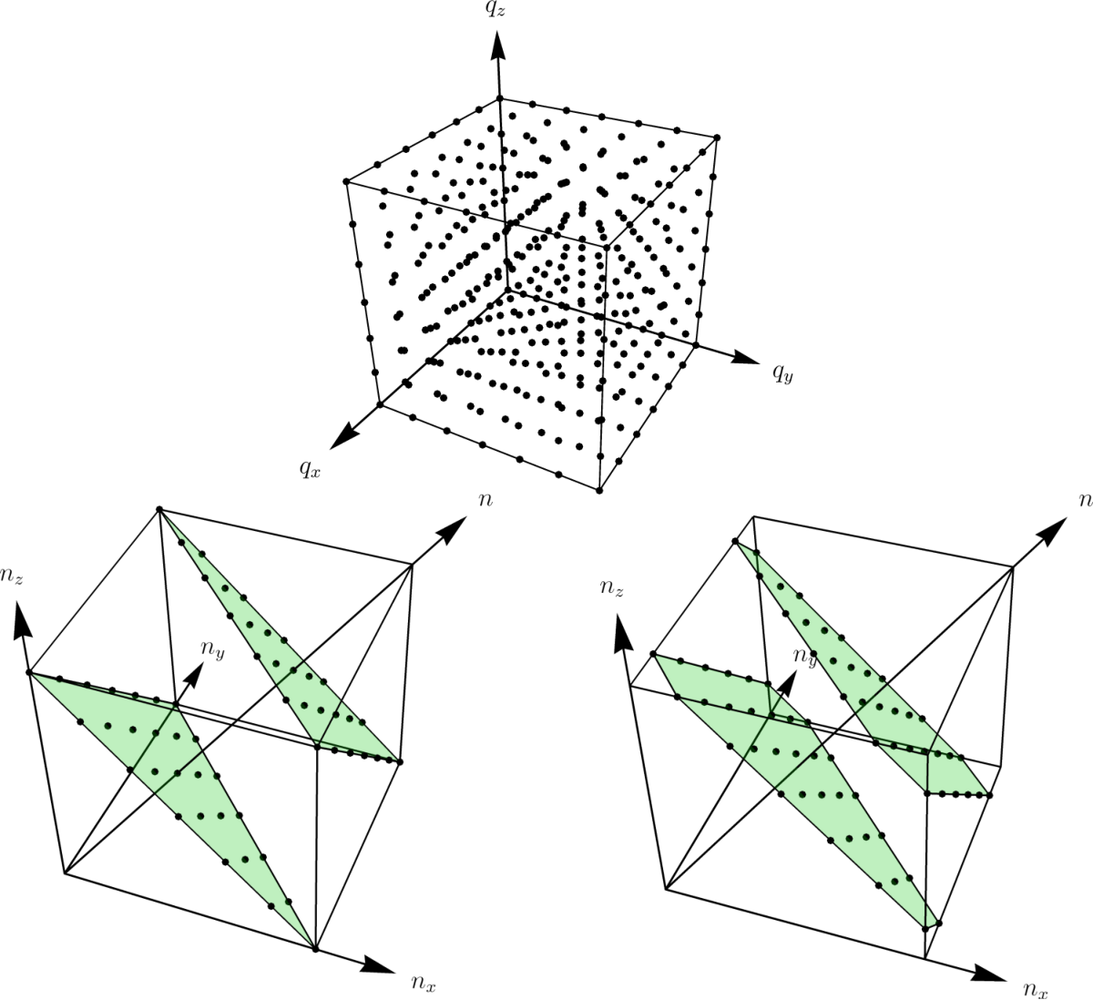
In the three dimensions that we now study, we have three sets of commuting $\hbox{\sf su($2$)}_{i}$ generators, $i\in\{x,y,z\}$, each giving position and mode (22) along the three space axes. We are here interested in the case where $j_{x}=j_{y}=j_{z}=:j$ so that we have a total of $N^{3}=(2j+1)^{3}$ states that we can represent as points in a cube of side $N$, which we picture in Fig. 1 (above). Modifying slightly the notation in (24) where subscripts denotes the related basis, we write the discrete and finite position states as $|\,q_{x},q_{y},q_{z}\,\rangle_{1}^{{\scriptscriptstyle(N)}}$. On the other hand, the discrete mode states, correspondingly written as $|\,n_{x},n_{y},n_{z}\,\rangle_{3}^{{\scriptscriptstyle(N)}}$ with $n_{i}|_{0}^{N-1}$, are pictured in Fig. 1 (below left-right) with the total mode number $n=n_{x}+n_{y}+n_{z}$ along the vertical axis, which ranges from $n=0$ at the bottom vertex, up to $n=3(N-1)=6j$ at the top vertex. A basis of $N^{3}$ discrete Cartesian wavefunctions is built from the $1D$ model in (24) simply as the direct product of the individual one-dimensional wavefunctions

These are orthonormal and complete bases for the $N^{3}$ space of ‘$3D$ images’, ‘voxels’, ‘signals’ or states on the discrete cube of Fig. 1. These act as unitary transformation matrix elements between the two bases depicted in that figure, i.e.,

where we remark that the basis for the modes $n_{i}$ is not so intuitive for visual representation, despite it has the same exact information that the basis of position $q_{i}$.

In the two-dimensional case examined in Refs. [2, 3], the position states are placed on an $N\times N$ square pixellated screen as shown in Fig. 2 (instead of the cube in Fig. 1), and the mode states are arranged in an $N\times N$ rhombus whose vertical axis is the total mode number $n=n_{x}+n_{y}$ and the horizontal axis is the mode difference $n_{x}-n_{y}$. The horizontal rungs in the rhombus, characterized by $n|_{0}^{2N-2}$, contain each $n+1$ members in the triangle that is the lower half of the rhombus $0\leq n\leq N{-}1=2j$, while the upper triangle $N\leq n\leq 2N{-}2=4j$ contains the high-mode components, whose members reflect the lower triangle. At this point, the importation of the su($2$) symmetry consists in taking these sets of $n+1$ states to be su($2$) multiplets, $|\,\lambda,\mu\,)$, of angular momentum $\lambda={\textstyle\frac{1}{2}}n$ and distinguished by the mode difference $\mu={\textstyle\frac{1}{2}}(n_{x}-n_{y})$, $\mu|_{-\lambda}^{\lambda}$. This holds for the states in the triangle in the lower half of the rhombus; the upper triangle is treated in the same way for $n\mapsto 4j-n$. Thereby, plane rotations by $\alpha$ in the $x$–$y$ plane of the pixellated screen are obtained from the well-defined rotations of the $|\,\lambda,\mu\,)$ basis states, which are only multiplied by $\exp({\rm i}\alpha\mu)$ .

Returning to the three-dimensional case examined here, we must import the continuous oscillator su($3$) symmetry algebra onto the finite oscillator mode states at each total mode level $n=n_{x}+n_{y}+n_{z}$ of Fig. 1; and then use its so($3$) subalgebra to define states which transform properly under rotations as in Eq. (20). In this case we have to slice the rhomboid-cube of modes into $n={}$ constant planes and see if and how we can accommodate them into $\hbox{\sf so($3$)}\subset\hbox{\sf su($3$)}$ multiplets. In slicing the cube in this way, we have now three regions to examine, instead of the two triangles of the $2D$ rhombus in Fig. 2.

Consider first the mode levels in the range $0\leq n\leq N-1$ where the slices of the cube yield triangular arrangements of $\tau_{n}$ points of side $n+1$, such as that shown in Fig. 1. These form completely symmetric (or bosonic) irreducible representations of su($3$), containing the multiplet of the states $|\,n_{x},n_{y},n_{z}\,\rangle$ of an ordinary quantum oscillator with $n$ energy quanta. These quanta can be shifted among the three axes by means of the nine u($3$) generators. These generators, ${\cal C}_{i}^{j}$, $i,j\in\{x,y,z\}$, are built in terms of three commuting sets of boson creation and annihilation operators, $\eta_{i},\,\xi_{j}$, fulfilling the commutators

In the vector space of these nine generators there is the invariant of total mode

which is at the center in the decomposition $\hbox{\sf u($3$)}=\hbox{\sf u($1$)}\oplus\hbox{\sf su($3$)}$ that determines this completely symmetric (bosonic) representation of su($3$) to be characterized by the single non-negative integer $n$.

Within the set of su($3$) generators (27) we find the subset that generates the rotation subalgebra $\hbox{\sf so($3$)}\subset\hbox{\sf su($3$)}$ of self-adjoint operators

whose commutation relations are $[{\cal L}_{i},{\cal L}_{j}]=-{\rm i}\,{\cal L}_{k}$ (with $i,\,j,\,k$ a cyclic permutation of $x,\,y,\,z$). The usual raising and lowering operators in so($3$) are

with $({\cal L}_{+})^{\dagger}={\cal L}_{-}$, and commutators $[{\cal L}_{z},{\cal L}_{\pm}]=\pm{\cal L}_{\pm}$ and $[{\cal L}_{+},{\cal L}_{-}]=-2{\cal L}_{0}\equiv-2{\cal L}_{z}$. The invariant Casimir operator is

The three commuting generators

yield the three labels of the $\tau_{n}$ Cartesian states $|\,n_{x},n_{y},n_{z}\,\rangle$, while the invariant ${\cal C}$ in (28), ${\cal L}^{2}$ in (31), and ${\cal L}_{z}$ in (29) determine the labels of the spherical basis $|\,n,\ell,m\,)$ with the ranges specified in (2) and shown in Fig. 1. The $+$ — $-$ mode difference $m:=n_{+}-n_{-}$, as in the $2D$ case, will have the role of angular momentum projection along the $z$–axis, provided that the $\tau_{n}$ points in set can be fitted into complete $\hbox{\sf so($3$)}\supset\hbox{\sf so($2$)}$ multiplets characterized by ranges $m|_{-\ell}^{\ell}$,i.e., those given by (2).

Figure 1 also provides a geometric proof that shows that there are complete so($3$) multiplets in any one of the levels $n|_{0}^{N-1}$ in the lower ‘inverted pyramid’ of finite-cube states. The lowest two rungs in the triangle of the figure contain $n+1$ and $n$ points respectively; when projected, on the $m={\textstyle\frac{1}{2}}(n_{x}-n_{y})$ axis they sum $2n+1$ points equidistant by unity, as if they were a multiplet of highest angular momentum $\ell=n$. Then come the next higher two rungs of $n-1$ and $n-2$ points, that project on $2n-3$ equidistant points, as if they belonged to a multiplet $\ell=n-2$. In the triangle of Fig. 1 the process continues with every two rungs yielding $\ell=n-4,\,n-6$, etc., ending with $\ell=1$ if $n$ is odd or, when $n$ is even, the projection of the single apex point, $m=0$ of $\ell=0$. Of course, only the two extreme pairs of points $\pm\mu=\ell=n$ and $\pm(m-1)$ are single and belong to that highest $\ell$; all other $m$’s will be linear combinations of the $\ell$’s that we projected out geometrically in this figure.

The symmetry importation on $0\leq n\leq N-1=2j$ consists in using the coefficients that bind the quantum harmonic oscillator Cartesian and spherical states; namely, the coefficients (17) given explicitly by Chacón and de Llano [5]. The slices in the upper pyramid of the cube of modes, for $4j=2(N-1)\leq n\leq 3(N-1)=6j$, yield reflected multiplets of ‘anti’-states, for which we may expect extra phases.

The $3D$ case is more complicated than the $2D$ one, because we also have to consider the intermediate range of total modes $N=2j+1\leq n\leq 4j-1=2N-3$. There, the $n$-slices of the mode cube are hexagons of generally unequal sides. We indicate by $(B,T)$ a hexagon with $B$ points on the base and $T$ points on the top. In particular, the $N$ triangles in the bottom pyramid ($n\in\{0,1,\ldots,N-1\}$) are $(n+1,1)$ in Fig. 1, and the $N$ inverted triangles in the top pyramid $(1,6j-n+1)$. The $N-2$ intermediate hexagons are thus $(N-1,2)$, $(N-2,3)$, $\ldots$, $(3,N-2)$, $(2,N-1)$. We have thus to ask whether the sets of points $(n_{x},n_{y},n_{z})$ in this intermediate region can be linearly combined into complete angular momentum multiplets, as those in the pyramid of Fig. 1 —or not. In Fig. 4 we show these intermediate slices for $N=7$ (a cube of $7^{3}=343$ voxels) that form the hexagons $(6,2)$ and $(5,3)$ for $n=6$ and $7$; the next two hexagons, $(3,5)$ and $(2,6)$ for $n=8$ and $9$, can be seen rotating the figure by 180^∘. We note that we can indeed project out complete multiplets $|\,\ell,m\,)$ of eigenstates where $m={\textstyle\frac{1}{2}}(n_{x}-n_{y})|_{-\ell}^{\ell}$, with linear combinations of $\ell\in\{5,\,4,\,2\}$ in the first hexagon and $\ell\in\{5,\,4,\,3\}$ in the second. As long as $N$ is even, we can scale up the figures to see that beyond the $(N,1)$ triangle at total mode $n=N-1$, in the first intermediate hexagon $(N-1,\,2)$ for $n=N$, the projected points will accommodate themselves into angular momentum multiplets $\ell\in\{N-1,\,N-2,N-4,\ldots,2\}$. For mode $n=N+1$, the hexagon $(N-2,\,3)$ will contain so($3$) multiplets $\ell\in\{N-1,\,N-2,\,N-3,\,N-5,\ldots,3\}$, and generally for $n=N+M$, the hexagon $(N-M+1,M)$ will contain $\ell\in\{N-1,\,N-2,\ldots,\,N-M\}\cap\{N-M-2,\,N-M-4,\ldots,M\}$.

References

- [1] Natig M. Atakishiyev, George S. Pogosyan, and Kurt Bernardo Wolf. Finite models of the oscillator. 2005.
- [2] Natig M Atakishiyev, George S Pogosyan, Luis Edgar Vicent, and Kurt Bernardo Wolf. Finite two-dimensional oscillator: II. the radial model. Journal of Physics A: Mathematical and General, 34(44):9399–9415, oct 2001.
- [3] Luis Edgar Vicent and Kurt Bernardo Wolf. Unitary transformation between cartesian- and polar-pixellated screens. Journal of the Optical Society of America A, 25(8):1875, jul 2008.
- [4] V. Bargmann and M. Moshinsky. Group theory of harmonic oscillators. Nuclear Physics, 18:697–712, August 1960.
- [5] E. Chacon and M. de Llano. Transformation brackets between cartesian and angular momentum harmonic oscillator basis functions with and without spin-orbit coupling tables for the – nuclear shell. Rev. Mex. Fix., 12, 1 1963.
- [6] R.R. Chasman and S. Wahlborn. Transformation scheme for harmonic-oscillator wave functions. Nuclear Physics A, 90(2):401–406, Jan 1967.
- [7] Natig M Atakishiyev, George S Pogosyan, Luis Edgar Vicent, and Kurt Bernardo Wolf. Finite two-dimensional oscillator: I. the cartesian model. Journal of Physics A: Mathematical and General, 34(44):9381–9398, oct 2001.
- [8] K. T. R. Davies and S. J. Krieger. Harmonic-oscillator transformation coefficients. Canadian Journal of Physics, 69(1):62–69, jan 1991.
- [9] M. Moshinsky and Yu.F. Smirnov. Harmonic Oscillator. 05 1996.
- [10] L. C. Biedenharn and James D. Louck. Angular Momentum in Quantum Physics. 12 1984.
- [11] Alejandro R. Urzúa and Kurt Bernardo Wolf. Unitary rotation and gyration of pixelated images on rectangular screens. Journal of the Optical Society of America A, 33(4):642, mar 2016.
- [12] Alejandro Urzua and Kurt Bernardo Wolf. Unitary rotation of pixellated polychromatic images. Journal of the Optical Society of America A, jun 2022.
- [13] Soo-Chang Pei and Chun-Lin Liu. Discrete spherical harmonic oscillator transforms on the cartesian grids using transformation coefficients. IEEE Transactions on Signal Processing, 61(5):1149–1164, mar 2013.
- [14] Soo-Chang Pei and Chun-Lin Liu. 3d rotation estimation using discrete spherical harmonic oscillator transforms. In 2014 IEEE International Conference on Acoustics, Speech and Signal Processing (ICASSP). IEEE, may 2014.
- [15] Guillermo Krötzsch, Kenan Uriostegui, and Kurt Bernardo Wolf. Unitary rotations in two-, three-, and d-dimensional cartesian data arrays. Journal of the Optical Society of America A, 31(7):1531, jun 2014.
- [16] Kurt Bernardo Wolf. Linear transformations and aberrations in continuous and finite systems. Journal of Physics A: Mathematical and Theoretical, 41(30):304026, jul 2008.