跳到论文正文
W Papers独立论文阅读器 arXiv:2207.12893 论文正文 计算阅读时间 · 0%
引用这篇论文根据当前论文元数据生成,正式投稿前建议核对。


License: arXiv.org perpetual non-exclusive license
arXiv:2207.12893v2 [hep-th] 12 Aug 2022

MITP/22-070

The three-loop equal-mass banana integral in ε\varepsilon-factorised form with meromorphic modular forms

Sebastian Pögel, Xing Wang and Stefan Weinzierl

PRISMA Cluster of Excellence, Institut für Physik,
Johannes Gutenberg-Universität Mainz,
D - 55099 Mainz, Germany

Abstract

We show that the differential equation for the three-loop equal-mass banana integral can be cast into an ε\varepsilon-factorised form with entries constructed from (meromorphic) modular forms and one special function, which can be given as an iterated integral of meromorphic modular forms. The ε\varepsilon-factorised form of the differential equation allows for a systematic solution to any order in the dimensional regularisation parameter ε\varepsilon. The alphabet of the iterated integrals contains six letters.

1 Introduction

For precision calculations in high-energy particle physics we need to evaluate Feynman integrals. It is a very interesting question which special functions appear in the final result of such a calculation. In the simplest case we find multiple polylogarithms [1, 2, 3, 4], which are iterated integrals of differential one-forms d​y/(y−c)dy/(y-c), where cc is a constant. An example is the one-loop bubble integral with equal non-zero masses. The equal-mass one-loop bubble integral can be expressed to all orders in the dimensional regularisation parameter ε\varepsilon in terms of multiple polylogarithms. A second non-trivial example is given by the massless two-loop double box integrals [5, 6].

More complicated Feynman integrals are related to elliptic curves and evaluate to iterated integrals of modular forms and/or specific differential one-forms related to the Kronecker function. The most prominent example is the two-loop sunrise integral with equal non-zero masses. The equal-mass two-loop sunrise integral can be expressed to all orders in the dimensional regularisation parameter ε\varepsilon in terms of iterated integrals of modular forms.

In this paper we consider the three-loop banana integral with equal non-zero masses. The three-loop banana integral is the next more complicated integral in the family of ll-loop banana integrals. The first two members of this family are the one-loop bubble integral and the two-loop sunrise integral. The geometry of the three-loop banana integral is related to a Calabi-Yau 22-fold (i.e. a surface) and thus more complicated than an elliptic Feynman integral, which in this context can be viewed as related to a Calabi-Yau 11-fold (i.e. a curve).

A convenient tool to obtain the result for a Feynman integral to any desired order in the dimensional regularisation parameter ε\varepsilon is the method of differential equations [7, 8, 9, 10]. For example, this method has been used at the beginning of the millennium to obtain the two-loop master integrals for γ∗→3​jets\gamma^{\ast}\rightarrow 3\;\mbox{jets} [11, 12]. The solution of the differential equation is significantly simplified, if the differential equation is in ε\varepsilon-factorised form [13]. If the differential equation is in ε\varepsilon-factorised form, we may read off the letters appearing in the iterated integrals from the differential equation. Such a form for the differential equation has been found for many Feynman integrals evaluating to multiple polylogarithms and selected examples of elliptic Feynman integrals [14, 15, 16]. In this paper we present the differential equation for the equal-mass three-loop banana integral in ε\varepsilon-factorised form.

The three-loop banana integral has been studied in the literature in the past [17, 18, 19, 20, 21, 22, 23] and we should carefully explain what is new in this article.

Let II be a vector of master integrals. The differential equation

d​I\displaystyle dI =\displaystyle= ε​A​I\displaystyle\varepsilon AI (1)

is said to be in ε\varepsilon-factorised form, if the connection matrix AA is independent of ε\varepsilon. An ε\varepsilon-factorised form can be achieved, if a full set of homogeneous solutions is known. The set of homogeneous solutions can be obtained by integrating the integrands of the master integrals over a set of independent contours [18]. This path has been followed in refs. [18, 24] and an ε\varepsilon-factorised form of the differential equation follows from the results of these papers. However, this is not the form we are interested in. It can be shown in the two-loop sunrise case that the solution for the Feynman integrals obtained in this way is not of uniform weight.

The first term of the ε\varepsilon-expansion of the three-loop banana integral (normalised to a homogeneous solution of the Picard-Fuchs operator) is known from ref. [17]. It corresponds to an Eichler integral

[I⁡(1,1,f4,τ)+43​ζ3]​ε3,\displaystyle\left[I\left(1,1,f_{4};\tau\right)+\frac{4}{3}\zeta_{3}\right]\varepsilon^{3}, (2)

where f4f_{4} is a modular form for Γ1​(6)\Gamma_{1}(6) of modular weight 44. The notation for iterated integrals is defined in sect. 6. In the main part of the paper f4f_{4} will be denoted as f4,af_{4,a}. This mirrors closely the first term of the ε\varepsilon-expansion of the two-loop sunrise integral (again normalised to a homogeneous solution of the appropriate Picard-Fuchs operator) [25, 14]

[4​I​(1,f3,τ)+3​C​l2​(2​π3)]​ε2,\displaystyle\left[4I\left(1,f_{3};\tau\right)+3\mathrm{Cl}_{2}\left(\frac{2\pi}{3}\right)\right]\varepsilon^{2}, (3)

where f3f_{3} is a modular form for Γ1​(6)\Gamma_{1}(6) of modular weight 33 and I⁡(1,f3,τ)I(1,f_{3};\tau) is again an Eichler integral. Cl2\mathrm{Cl}_{2} denotes the Clausen function. We are interested in the higher-order terms in the dimensional regularisation parameter ε\varepsilon which add to eq. (2). This has been considered in ref. [20], where it was shown that the higher-order terms are given by iterated integrals of meromorphic modular forms. The authors of this reference also gave a differential equation. However this differential equation is not ε\varepsilon-factorised, as it contains an additional 1/ε1/\varepsilon-term. In this paper we improve the situation by deriving a differential equation in ε\varepsilon-factorised form.

At first sight it seems surprising that the three-loop banana integral can be expressed in terms of iterated integrals of (meromorphic) modular forms as the geometry is related to a Calabi-Yau 22-fold and not an elliptic curve. However it has been known for a long time that the corresponding Picard-Fuchs operator (a third-order differential operator) is the symmetric square of a second-order differential operator [26, 27]. By a variable transformation, this second-order differential operator is related to the Picard-Fuchs operator of the two-loop sunrise integral [17, 19]. We start with the dimensionless kinematic variable x=p2/m2x=p^{2}/m^{2}. The variable transformation maps the pseudo-threshold x=4x=4 and the threshold x=16x=16 of the three-loop banana integral to the points y=3y=3 and y=−3y=-3, respectively. The variable yy is the natural “physical” variable in the sunrise context. Mapped to the complex upper half-plane, these points correspond to τ=14​(1+i​3)\tau=\frac{1}{4}(1+i\sqrt{3}) and τ=16​(3+i​3)\tau=\frac{1}{6}(3+i\sqrt{3}), respectively. At these points the elliptic curve of the two-loop sunrise integral is not degenerate. As the original differential equation for the three-loop banana integral has singularities at these points, meromorphic modular forms (with poles at τ=14​(1+i​3)\tau=\frac{1}{4}(1+i\sqrt{3}) and τ=16​(3+i​3)\tau=\frac{1}{6}(3+i\sqrt{3})) emerge naturally [28, 20]. We show that the ε\varepsilon-factorised differential equation has at most simple poles at these points.

This paper is organised as follows: In section 2 we define the three-loop banana integral and the associated Picard-Fuchs operator. In section 3 we construct from an ansatz a set of master integrals which lead to an ε\varepsilon-factorised differential equation. This ansatz follows closely the steps taken in ref. [14, 15, 16]. In section 4 we define the periods for the elliptic curve of the two-loop sunrise integral. From these periods we can construct a solution for the Picard-Fuchs operator of the three-loop banana integral. In section 5 we introduce (meromorphic) modular forms. We only need four (meromorphic) modular forms of modular weight 11 as basic building blocks, which we label

b0,b1,b3,b−3.\displaystyle b_{0},\;\;\;b_{1},\;\;\;b_{3},\;\;\;b_{-3}. (4)

All other occurring (meromorphic) modular forms are polynomials in these. In section 6 we introduce the notation for iterated integrals of (meromorphic) modular forms. In section 7 we present the differential equation for the master integrals in ε\varepsilon-factorised form. The differential equation contains six letters, which we denote as

1,f2,a,f2,b,f4,a,f4,b,f6.\displaystyle 1,\;\;\;f_{2,a},\;\;\;f_{2,b},\;\;\;f_{4,a},\;\;\;f_{4,b},\;\;\;f_{6}. (5)

The transformation laws of the entries of the differential equation under modular transformations of Γ1​(6)\Gamma_{1}(6) are discussed in section 8. The differential equation is solved in section 9 and analytical results for all master integrals up to order ε4\varepsilon^{4} are presented. In section 10 we give numerical results and show that they agree with results obtained from SecDec [29, 30, 31]. Our conclusions are presented in section 11. In appendix A we derive the boundary conditions necessary for solving the differential equation. Appendix B describes the supplementary electronic file attached to this article, which gives the solution for the banana integrals up to order ε6\varepsilon^{6}.

2 Definitions

Refer to caption
Figure 1: The three-loop banana graph.

We are interested in the integrals

Iν1​ν2​ν3​ν4\displaystyle I_{\nu_{1}\nu_{2}\nu_{3}\nu_{4}} =\displaystyle= e3​γE​ε​(m2)ν−32​D​∫(∏a=14dD​kai​πD2)​i​πD2​δD​(p−∑b=14kb)​(∏c=141(−kc2+m2)νc)\displaystyle e^{3\gamma_{E}\varepsilon}\left(m^{2}\right)^{\nu-\frac{3}{2}D}\int\left(\prod\limits_{a=1}^{4}\frac{d^{D}k_{a}}{i\pi^{\frac{D}{2}}}\right)i\pi^{\frac{D}{2}}\delta^{D}\left(p-\sum\limits_{b=1}^{4}k_{b}\right)\left(\prod\limits_{c=1}^{4}\frac{1}{\left(-k_{c}^{2}+m^{2}\right)^{\nu_{c}}}\right) (6)

where DD denotes the number of space-time dimensions, ε\varepsilon the dimensional regularisation parameter, γE\gamma_{E} the Euler-Mascheroni constant and the quantity ν\nu is defined by

ν\displaystyle\nu =\displaystyle= ∑j=14νj.\displaystyle\sum\limits_{j=1}^{4}\nu_{j}. (7)

We consider these integrals in D=2−2​εD=2-2\varepsilon space-time dimensions. It is convenient to introduce the dimensionless variable

x\displaystyle x =\displaystyle= p2m2.\displaystyle\frac{p^{2}}{m^{2}}. (8)

It is well-known that this family of Feynman integrals has four master integrals. A possible choice for a basis of master integrals is

I1110,I1111,I1112,I1113.\displaystyle I_{1110},\;I_{1111},\;I_{1112},\;I_{1113}. (9)

The Feynman integral I1110I_{1110} is a product of three one-loop tadpole integrals and rather simple. We set

I1\displaystyle I_{1} =\displaystyle= ε3​I1110=[eγE​ε​Γ​(1+ε)]3.\displaystyle\varepsilon^{3}I_{1110}\;=\;\left[e^{\gamma_{E}\varepsilon}\Gamma\left(1+\varepsilon\right)\right]^{3}. (10)

The integral I1I_{1} has uniform weight. For I1111I_{1111} we have the inhomogeneous third-order differential equation

L3​I1111\displaystyle L_{3}\;I_{1111} =\displaystyle= −24​ε3x2​(x−4)​(x−16)​I1110,\displaystyle-\frac{24\varepsilon^{3}}{x^{2}\left(x-4\right)\left(x-16\right)}I_{1110}, (11)

with

L3\displaystyle L_{3} =\displaystyle= d3d​x3+[3x+3​(1+2​ε)2​(x−4)+3​(1+2​ε)2​(x−16)]​d2d​x2\displaystyle\frac{d^{3}}{dx^{3}}+\left[\frac{3}{x}+\frac{3\left(1+2\varepsilon\right)}{2\left(x-4\right)}+\frac{3\left(1+2\varepsilon\right)}{2\left(x-16\right)}\right]\frac{d^{2}}{dx^{2}} (12)
+[7​x2−68​x+64x2​(x−4)​(x−16)+6​ε​(3​x−20)x​(x−4)​(x−16)+ε2​(11​x+16)x2​(x−16)]​dd​x\displaystyle+\left[\frac{7x^{2}-68x+64}{x^{2}\left(x-4\right)\left(x-16\right)}+\frac{6\varepsilon\left(3x-20\right)}{x\left(x-4\right)\left(x-16\right)}+\frac{\varepsilon^{2}\left(11x+16\right)}{x^{2}\left(x-16\right)}\right]\frac{d}{dx}
+(1+2​ε)​(1+3​ε)​[1x2​(x−16)+ε⁡(x+2)x2​(x−4)​(x−16)].\displaystyle+\left(1+2\varepsilon\right)\left(1+3\varepsilon\right)\left[\frac{1}{x^{2}\left(x-16\right)}+\frac{\varepsilon\left(x+2\right)}{x^{2}\left(x-4\right)\left(x-16\right)}\right].

We denote by L3(0)L_{3}^{(0)} the ε\varepsilon-independent part of L3L_{3} [32]:

L3(0)=d3d​x3+[3x+32​(x−4)+32​(x−16)]​d2d​x2+7​x2−68​x+64x2​(x−4)​(x−16)​dd​x+1x2​(x−16).\displaystyle L_{3}^{(0)}=\frac{d^{3}}{dx^{3}}+\left[\frac{3}{x}+\frac{3}{2\left(x-4\right)}+\frac{3}{2\left(x-16\right)}\right]\frac{d^{2}}{dx^{2}}+\frac{7x^{2}-68x+64}{x^{2}\left(x-4\right)\left(x-16\right)}\frac{d}{dx}+\frac{1}{x^{2}\left(x-16\right)}. (13)

Let

L2(0)\displaystyle L_{2}^{(0)} =\displaystyle= d2d​x2+[1x+12​(x−4)+12​(x−16)]​dd​x+(x−8)4​x​(x−4)​(x−16).\displaystyle\frac{d^{2}}{dx^{2}}+\left[\frac{1}{x}+\frac{1}{2\left(x-4\right)}+\frac{1}{2\left(x-16\right)}\right]\frac{d}{dx}+\frac{\left(x-8\right)}{4x\left(x-4\right)\left(x-16\right)}. (14)

The differential operator L3(0)L_{3}^{(0)} is the symmetric product of L2(0)L_{2}^{(0)} [26]: If ψ1,ψ2\psi_{1},\psi_{2} are two independent solutions of L2(0)L_{2}^{(0)}

L2(0)​ψi\displaystyle L_{2}^{(0)}\;\psi_{i} =\displaystyle= 0,i∈{1,2},\displaystyle 0,\;\;\;\;\;\;i\;\in\;\{1,2\}, (15)

then the solution space of L3(0)L_{3}^{(0)} is spanned by

ψ12,ψ1​ψ2,ψ22.\displaystyle\psi_{1}^{2},\;\;\psi_{1}\psi_{2},\;\;\psi_{2}^{2}. (16)

The Wronskian is defined by

W\displaystyle W =\displaystyle= ψ1​dd​x​ψ2−ψ2​dd​x​ψ1.\displaystyle\psi_{1}\frac{d}{dx}\psi_{2}-\psi_{2}\frac{d}{dx}\psi_{1}. (17)

We have

[dd​x+1x+12​(x−4)+12​(x−16)]​W\displaystyle\left[\frac{d}{dx}+\frac{1}{x}+\frac{1}{2\left(x-4\right)}+\frac{1}{2\left(x-16\right)}\right]W =\displaystyle= 0\displaystyle 0 (18)

and

W\displaystyle W =\displaystyle= 2​π​i​cx​(4−x)12​(16−x)12,\displaystyle\frac{2\pi ic}{x\left(4-x\right)^{\frac{1}{2}}\left(16-x\right)^{\frac{1}{2}}}, (19)

where cc is a constant. The constant cc depends on the normalisation of the two independent solutions ψ1\psi_{1} and ψ2\psi_{2}. In section 4 we give explicit expressions for the two independent solutions of eq. (15). This choice of solutions yields c=3c=3.

3 Master integrals

In this section we determine a choice of master integrals, which put the differential equation into an ε\varepsilon-form. We do this in two steps: In the first step we start from a rather general ansatz with five unknown functions. We derive differential equations these functions have to satisfy from the condition that the differential equation for the master integrals is in ε\varepsilon-form. Four of these five functions are easily solved for, leading to a more specific ansatz, which we consider in step 22. This specific ansatz involves only one unknown function. We determine this remaining function in section 3.2.

3.1 Step 1

Let ω1\omega_{1}, JJ, F32F_{32}, F42F_{42} and F43F_{43} be (a priori unknown) functions of xx. Here, JJ denotes the Jacobian for a (a priori unknown) change of variable from xx to τ\tau:

J\displaystyle J =\displaystyle= d​xd​τ.\displaystyle\frac{dx}{d\tau}. (20)

This implies

dd​τ\displaystyle\frac{d}{d\tau} =\displaystyle= J​dd​x.\displaystyle J\frac{d}{dx}. (21)

We start from the following ansatz for the master integrals

I1\displaystyle I_{1} =\displaystyle= ε3​I1110,\displaystyle\varepsilon^{3}I_{1110},
I2\displaystyle I_{2} =\displaystyle= ε3​π2ω1​I1111,\displaystyle\varepsilon^{3}\frac{\pi^{2}}{\omega_{1}}I_{1111},
I3\displaystyle I_{3} =\displaystyle= 12​π​i​ε​dd​τ​I2+F32​I2,\displaystyle\frac{1}{2\pi i\varepsilon}\frac{d}{d\tau}I_{2}+F_{32}I_{2},
I4\displaystyle I_{4} =\displaystyle= 12​π​i​ε​dd​τ​I3+F42​I2+F43​I3.\displaystyle\frac{1}{2\pi i\varepsilon}\frac{d}{d\tau}I_{3}+F_{42}I_{2}+F_{43}I_{3}. (22)

The differential equation for this set of master integrals is in ε\varepsilon-form

d​I\displaystyle dI =\displaystyle= ε​A​I,\displaystyle\varepsilon AI, (23)

provided the following set of six differential equations for the functions ω1\omega_{1}, JJ, F32F_{32}, F42F_{42}, F43F_{43} hold: For ω1\omega_{1} we require the two equations

L3(0)​ω1=0,\displaystyle L_{3}^{(0)}\;\omega_{1}=0, (24)
1ω1​d2​ω1d​x2−12​(1ω1​d​ω1d​x)2+2​(x2−15​x+32)x​(x−4)​(x−16)​1ω1​d​ω1d​x+(x−8)2​x​(x−4)​(x−16)=0.\displaystyle\frac{1}{\omega_{1}}\frac{d^{2}\omega_{1}}{dx^{2}}-\frac{1}{2}\left(\frac{1}{\omega_{1}}\frac{d\omega_{1}}{dx}\right)^{2}+\frac{2\left(x^{2}-15x+32\right)}{x\left(x-4\right)\left(x-16\right)}\frac{1}{\omega_{1}}\frac{d\omega_{1}}{dx}+\frac{\left(x-8\right)}{2x\left(x-4\right)\left(x-16\right)}=0. (25)

For JJ we require

d​ln⁡Jd​x\displaystyle\frac{d\ln J}{dx} =\displaystyle= d​ln⁡ω1d​x+2​(x2−15​x+32)x​(x−4)​(x−16).\displaystyle\frac{d\ln\omega_{1}}{dx}+\frac{2\left(x^{2}-15x+32\right)}{x\left(x-4\right)\left(x-16\right)}. (26)

For F32F_{32}, F42F_{42}, F43F_{43} we require

d2​F32d​x2+[d​ln⁡ω1d​x+2​(x2−15​x+32)x​(x−4)​(x−16)]d​F32d​x+3​J2​π​i[−(x−10)(x−4)​(x−16)(d​ln⁡ω1d​x)2\displaystyle\frac{d^{2}F_{32}}{dx^{2}}+\left[\frac{d\ln\omega_{1}}{dx}+\frac{2\left(x^{2}-15x+32\right)}{x\left(x-4\right)\left(x-16\right)}\right]\frac{dF_{32}}{dx}+\frac{3J}{2\pi i}\left[-\frac{\left(x-10\right)}{\left(x-4\right)\left(x-16\right)}\left(\frac{d\ln\omega_{1}}{dx}\right)^{2}\right.
−2​(x3−30​x2+228​x−640)x​(x−4)2​(x−16)2d​ln⁡ω1d​x−(x3−28​x2+168​x−384)x2​(x−4)2​(x−16)2]=0,\displaystyle\left.-\frac{2\left(x^{3}-30x^{2}+228x-640\right)}{x\left(x-4\right)^{2}\left(x-16\right)^{2}}\frac{d\ln\omega_{1}}{dx}-\frac{\left(x^{3}-28x^{2}+168x-384\right)}{x^{2}\left(x-4\right)^{2}\left(x-16\right)^{2}}\right]=0,
d​F42d​x−3​F32​d​F32d​x+3​J2​π​i​2​(x−10)(x−4)​(x−16)​d​F32d​x\displaystyle\frac{dF_{42}}{dx}-3F_{32}\frac{dF_{32}}{dx}+\frac{3J}{2\pi i}\frac{2\left(x-10\right)}{\left(x-4\right)\left(x-16\right)}\frac{dF_{32}}{dx} (27)
+3​J2​π​i​[2​(x−10)(x−4)​(x−16)​d​ln⁡ω1d​x+2​(x3−30​x2+228​x−640)x​(x−4)2​(x−16)2]​F32\displaystyle+\frac{3J}{2\pi i}\left[\frac{2\left(x-10\right)}{\left(x-4\right)\left(x-16\right)}\frac{d\ln\omega_{1}}{dx}+\frac{2\left(x^{3}-30x^{2}+228x-640\right)}{x\left(x-4\right)^{2}\left(x-16\right)^{2}}\right]F_{32}
+J2(2​π​i)2​[−(11​x+16)x2​(x−16)​d​ln⁡ω1d​x−(11​x−14)x2​(x−4)​(x−16)]=0,\displaystyle+\frac{J^{2}}{\left(2\pi i\right)^{2}}\left[-\frac{\left(11x+16\right)}{x^{2}\left(x-16\right)}\frac{d\ln\omega_{1}}{dx}-\frac{\left(11x-14\right)}{x^{2}\left(x-4\right)\left(x-16\right)}\right]=0,
d​F43d​x+2​d​F32d​x+3​J2​π​i​[−2​(x−10)(x−4)​(x−16)​d​ln⁡ω1d​x−2​(x3−30​x2+228​x−640)x​(x−4)2​(x−16)2]=0.\displaystyle\frac{dF_{43}}{dx}+2\frac{dF_{32}}{dx}+\frac{3J}{2\pi i}\left[-\frac{2\left(x-10\right)}{\left(x-4\right)\left(x-16\right)}\frac{d\ln\omega_{1}}{dx}-\frac{2\left(x^{3}-30x^{2}+228x-640\right)}{x\left(x-4\right)^{2}\left(x-16\right)^{2}}\right]=0.

These differential equations follow from the requirement that terms of order εj\varepsilon^{j} with j≠1j\neq 1 are absent in the differential equation for the master integrals: Eq. (24) removes the ε−2\varepsilon^{-2}-term of A4,2A_{4,2}. Eq. (26) removes the ε0\varepsilon^{0}-term of A4,4A_{4,4}. Eq. (25) (together with the previous two equations) removes the ε−1\varepsilon^{-1}-term of A4,3A_{4,3}. F32F_{32} removes the ε−1\varepsilon^{-1}-term of A4,2A_{4,2}, F42F_{42} removes the ε0\varepsilon^{0}-term of A4,2A_{4,2} and F43F_{43} removes the ε0\varepsilon^{0}-term of A4,3A_{4,3}.

With

d2​ln⁡ω1d​x2\displaystyle\frac{d^{2}\ln\omega_{1}}{dx^{2}} =\displaystyle= 1ω1​d2​ω1d​x2−(1ω1​d​ω1d​x)2\displaystyle\frac{1}{\omega_{1}}\frac{d^{2}\omega_{1}}{dx^{2}}-\left(\frac{1}{\omega_{1}}\frac{d\omega_{1}}{dx}\right)^{2} (28)

we may write eq. (25) alternatively as

d2​ln⁡ω1d​x2+12​(d​ln⁡ω1d​x)2+2​(x2−15​x+32)x​(x−4)​(x−16)​d​ln⁡ω1d​x+(x−8)2​x​(x−4)​(x−16)\displaystyle\frac{d^{2}\ln\omega_{1}}{dx^{2}}+\frac{1}{2}\left(\frac{d\ln\omega_{1}}{dx}\right)^{2}+\frac{2\left(x^{2}-15x+32\right)}{x\left(x-4\right)\left(x-16\right)}\frac{d\ln\omega_{1}}{dx}+\frac{\left(x-8\right)}{2x\left(x-4\right)\left(x-16\right)} =\displaystyle= 0.\displaystyle 0. (29)

We have to check that eq. (24) and eq. (25) together have a solution. The following lemma ensures this:

Lemma 1.

Assume that ω1\omega_{1} satisfies eq. (25). Then

L3(0)​ω1\displaystyle L_{3}^{(0)}\;\omega_{1} =\displaystyle= 0.\displaystyle 0. (30)
Proof.

To prove this lemma, one verifies that the left-hand side of eq. (24) simplifies to zero with the relation eq. (25). ∎

Thus it is sufficient to just consider the second-order non-linear inhomogeneous differential equation eq. (25) (or equivalently eq. (29)) and ignore eq. (24).

It is not too difficult to solve eq. (29): We know that any solution of eq. (29) is automatically a solution of eq. (24). The solution space of eq. (24) is given by

c1​ψ12+c2​ψ1​ψ2+c3​ψ22\displaystyle c_{1}\psi_{1}^{2}+c_{2}\psi_{1}\psi_{2}+c_{3}\psi_{2}^{2} (31)

with unknown constants c1,c2,c3c_{1},c_{2},c_{3}.

Lemma 2.

Let ψ\psi be a solution of eq. (15). Then ψ2\psi^{2} is a solution of eq. (29).

Proof.

To prove this lemma, one verifies that the left-hand side of eq. (29) simplifies to zero with the relation eq. (15). ∎

In other words, ω1\omega_{1} needs to be a perfect square and of the form given in eq. (31). Thus,

ψ12,ψ22\displaystyle\psi_{1}^{2},\;\;\psi_{2}^{2} (32)

are solutions of eq. (29), while ψ1​ψ2\psi_{1}\psi_{2} is not.

From now on we set

ω1\displaystyle\omega_{1} =\displaystyle= ψ12.\displaystyle\psi_{1}^{2}. (33)

Let us now turn to the Jacobian JJ. It is easier to work with

J−1\displaystyle J^{-1} =\displaystyle= d​τd​x.\displaystyle\frac{d\tau}{dx}. (34)

We may rewrite eq. (26) as

d​ln⁡J−1d​x+d​ln⁡ω1d​x+2​(x2−15​x+32)x​(x−4)​(x−16)\displaystyle\frac{d\ln J^{-1}}{dx}+\frac{d\ln\omega_{1}}{dx}+\frac{2\left(x^{2}-15x+32\right)}{x\left(x-4\right)\left(x-16\right)} =\displaystyle= 0.\displaystyle 0. (35)

It is easily verified that

τ\displaystyle\tau =\displaystyle= ψ2ψ1\displaystyle\frac{\psi_{2}}{\psi_{1}} (36)

solves eq. (35). We then have

J−1\displaystyle J^{-1} =\displaystyle= Wψ12.\displaystyle\frac{W}{\psi_{1}^{2}}. (37)

3.2 Step 2

With the information gathered so far

ω1=ψ12,\displaystyle\omega_{1}\;=\;\psi_{1}^{2}, J=ψ12W,\displaystyle J\;=\;\frac{\psi_{1}^{2}}{W}, (38)

we may clean-up our ansatz. The differential equations for F42F_{42} and F43F_{43} are of first order and easily solved. Our ansatz reduces to

I1\displaystyle I_{1} =\displaystyle= ε3​I1110,\displaystyle\varepsilon^{3}I_{1110},
I2\displaystyle I_{2} =\displaystyle= ε3​π2ψ12​I1111,\displaystyle\varepsilon^{3}\frac{\pi^{2}}{\psi_{1}^{2}}I_{1111},
I3\displaystyle I_{3} =\displaystyle= 12​π​i​ε​dd​τ​I2+[F2−π​i​(x−10)(x−4)​(x−16)​W​(ψ1π)2]​I2,\displaystyle\frac{1}{2\pi i\varepsilon}\frac{d}{d\tau}I_{2}+\left[F_{2}-\frac{\pi i\left(x-10\right)}{\left(x-4\right)\left(x-16\right)W}\left(\frac{\psi_{1}}{\pi}\right)^{2}\right]I_{2},
I4\displaystyle I_{4} =\displaystyle= 12​π​i​ε​dd​τ​I3+[32​F22+π2​(x+8)2​(x2−8​x+64)8​x2​(x−4)2​(x−16)2​W2​(ψ1π)4]​I2\displaystyle\frac{1}{2\pi i\varepsilon}\frac{d}{d\tau}I_{3}+\left[\frac{3}{2}F_{2}^{2}+\frac{\pi^{2}\left(x+8\right)^{2}\left(x^{2}-8x+64\right)}{8x^{2}\left(x-4\right)^{2}\left(x-16\right)^{2}W^{2}}\left(\frac{\psi_{1}}{\pi}\right)^{4}\right]I_{2} (39)
+[−2​F2−π​i​(x−10)(x−4)​(x−16)​W​(ψ1π)2]​I3\displaystyle+\left[-2F_{2}-\frac{\pi i\left(x-10\right)}{\left(x-4\right)\left(x-16\right)W}\left(\frac{\psi_{1}}{\pi}\right)^{2}\right]I_{3}

with one unknown function F2F_{2}, which satisfies

d2​F2d​x2+[2​(x2−15​x+32)x​(x−4)​(x−16)+2​(d​ln⁡ψ1d​x)]​d​F2d​x\displaystyle\frac{d^{2}F_{2}}{dx^{2}}+\left[\frac{2\left(x^{2}-15x+32\right)}{x\left(x-4\right)\left(x-16\right)}+2\left(\frac{d\ln\psi_{1}}{dx}\right)\right]\frac{dF_{2}}{dx} =\displaystyle= π​i​(x−8)​(x+8)3x2​(x−4)3​(x−16)3​W​(ψ1π)2.\displaystyle\frac{\pi i\left(x-8\right)\left(x+8\right)^{3}}{x^{2}\left(x-4\right)^{3}\left(x-16\right)^{3}W}\left(\frac{\psi_{1}}{\pi}\right)^{2}. (40)

This is a linear inhomogeneous first-order differential equation for F2′F_{2}^{\prime}. Noting that

2​(x2−15​x+32)x​(x−4)​(x−16)+2​(d​ln⁡ψ1d​x)\displaystyle\frac{2\left(x^{2}-15x+32\right)}{x\left(x-4\right)\left(x-16\right)}+2\left(\frac{d\ln\psi_{1}}{dx}\right) =\displaystyle= d​ln⁡Jd​x\displaystyle\frac{d\ln J}{dx} (41)

one finds

F2′\displaystyle F_{2}^{\prime} =\displaystyle= J−1​[C2+∫d​x​J​π​i​(x−8)​(x+8)3x2​(x−4)3​(x−16)3​W​(ψ1π)2]\displaystyle J^{-1}\left[C_{2}+\int dx\;J\frac{\pi i\left(x-8\right)\left(x+8\right)^{3}}{x^{2}\left(x-4\right)^{3}\left(x-16\right)^{3}W}\left(\frac{\psi_{1}}{\pi}\right)^{2}\right] (42)

and

F2\displaystyle F_{2} =\displaystyle= C1+C2​τ+(2​π​i)2​∫d​τ​∫d​τ​x⁡(x−8)​(x+8)3864​(4−x)32​(16−x)32​(ψ1π)6.\displaystyle C_{1}+C_{2}\tau+\left(2\pi i\right)^{2}\int d\tau\int d\tau\;\frac{x\left(x-8\right)\left(x+8\right)^{3}}{864\left(4-x\right)^{\frac{3}{2}}\left(16-x\right)^{\frac{3}{2}}}\left(\frac{\psi_{1}}{\pi}\right)^{6}. (43)

We only need one specific solution. We may therefore set the integration constants to zero. This yields

F2\displaystyle F_{2} =\displaystyle= (2​π​i)2​∫i​∞τd​τ1​∫i​∞τ1d​τ2​x⁡(x−8)​(x+8)3864​(4−x)32​(16−x)32​(ψ1π)6,\displaystyle\left(2\pi i\right)^{2}\int\limits_{i\infty}^{\tau}d\tau_{1}\int\limits_{i\infty}^{\tau_{1}}d\tau_{2}\;\frac{x\left(x-8\right)\left(x+8\right)^{3}}{864\left(4-x\right)^{\frac{3}{2}}\left(16-x\right)^{\frac{3}{2}}}\left(\frac{\psi_{1}}{\pi}\right)^{6}, (44)

where the integrand is viewed as a function of τ2\tau_{2}. We denote the integrand by

g6\displaystyle g_{6} =\displaystyle= x⁡(x−8)​(x+8)3864​(4−x)32​(16−x)32​(ψ1π)6.\displaystyle\frac{x\left(x-8\right)\left(x+8\right)^{3}}{864\left(4-x\right)^{\frac{3}{2}}\left(16-x\right)^{\frac{3}{2}}}\left(\frac{\psi_{1}}{\pi}\right)^{6}. (45)

We note that the definition of F2F_{2} depends on the integration path. Later on we will expand the integrand in a q¯\bar{q}-series. As long as we stay inside the region of convergence of the q¯\bar{q}-series we may suppress the dependence on the integration path. We are only interested in this case and we therefore do not write the dependence on the integration path explicitly. The dependence on the integration path is relevant as soon as we analytically continue F2F_{2} beyond the region of convergence of the q¯\bar{q}-series. Later on we will see that the radius of convergence of the q¯\bar{q}-series is set by the threshold singularity at x=16x=16, corresponding to τ=1/2+i​3/6\tau=1/2+i\sqrt{3}/6. As long as

Im​τ>36\displaystyle\mathrm{Im}\;\tau\;>\;\frac{\sqrt{3}}{6}    or    |q¯|<e−π3​3\displaystyle\left|\bar{q}\right|<e^{-\frac{\pi}{3}\sqrt{3}} (46)

we do not have to worry about the path dependence.

4 The periods

In this section we consider the two solutions ψ1\psi_{1} and ψ2\psi_{2} of eq. (15). It is well-known that these solutions are related to the two periods ψ1sunrise\psi_{1}^{\mathrm{sunrise}} and ψ2sunrise\psi_{2}^{\mathrm{sunrise}} of the sunrise integral. In this section we review the construction.

The first step is the variable transformation

x=−(y−1)​(y−9)y,\displaystyle x\;=\;-\frac{\left(y-1\right)\left(y-9\right)}{y}, y=12​[10−x−4−x​16−x].\displaystyle y\;=\;\frac{1}{2}\left[10-x-\sqrt{4-x}\sqrt{16-x}\right]. (47)

In expressing yy as a function of xx, we made a choice for the sign of the square root. With this choice the value x=0x=0 is mapped to y=1y=1. This transformation rationalises the square root

4−x​16−x\displaystyle\sqrt{4-x}\sqrt{16-x} =\displaystyle= −(y+3)​(y−3)y.\displaystyle-\frac{\left(y+3\right)\left(y-3\right)}{y}. (48)

The sign is fixed by eq. (47). This is most easily seen as follows: In the Euclidean region (i.e. x∈]−∞,0]x\in]-\infty,0] and y∈[0,1]y\in[0,1]) both sides of eq, (48) are positive.

In terms of the variable yy, eq. (15) transforms into

[d2d​y2+(1y−1+1y−9)​dd​y+y2−2​y+94​y2​(y−1)​(y−9)]​ψi\displaystyle\left[\frac{d^{2}}{dy^{2}}+\left(\frac{1}{y-1}+\frac{1}{y-9}\right)\frac{d}{dy}+\frac{y^{2}-2y+9}{4y^{2}\left(y-1\right)\left(y-9\right)}\right]\psi_{i} =\displaystyle= 0.\displaystyle 0. (49)

If we now make the ansatz

ψi\displaystyle\psi_{i} =\displaystyle= y​ψisunrise\displaystyle\sqrt{y}\;\psi_{i}^{\mathrm{sunrise}} (50)

we find for ψisunrise\psi_{i}^{\mathrm{sunrise}} the differential equation

[d2d​y2+(1y+1y−1+1y−9)​dd​y+y−3y​(y−1)​(y−9)]​ψisunrise\displaystyle\left[\frac{d^{2}}{dy^{2}}+\left(\frac{1}{y}+\frac{1}{y-1}+\frac{1}{y-9}\right)\frac{d}{dy}+\frac{y-3}{y\left(y-1\right)\left(y-9\right)}\right]\psi_{i}^{\mathrm{sunrise}} =\displaystyle= 0.\displaystyle 0. (51)

This is the differential equation for the periods of the sunrise integral. The solutions are well-known: We consider an elliptic curve defined by the quartic polynomial

E\displaystyle E :\displaystyle: v2−(u−u1)​(u−u2)​(u−u3)​(u−u4)= 0,\displaystyle v^{2}-\left(u-u_{1}\right)\left(u-u_{2}\right)\left(u-u_{3}\right)\left(u-u_{4}\right)\;=\;0, (52)

where the uju_{j} (with j∈{1,2,3,4}j\in\{1,2,3,4\}) denote the roots of the quartic polynomial. The roots uju_{j} are given by

u1=−4,u2=−(1+y)2,u3=−(1−y)2,u4= 0.\displaystyle u_{1}\;=\;-4,\;\;\;\;\;\;u_{2}\;=\;-\left(1+\sqrt{y}\right)^{2},\;\;\;\;\;\;u_{3}\;=\;-\left(1-\sqrt{y}\right)^{2},\;\;\;\;\;\;u_{4}\;=\;0. (53)

We set

U1=(u3−u2)​(u4−u1),U2=(u2−u1)​(u4−u3),U3=(u3−u1)​(u4−u2).\displaystyle U_{1}\;=\;\left(u_{3}-u_{2}\right)\left(u_{4}-u_{1}\right),\;\;\;\;\;\;U_{2}\;=\;\left(u_{2}-u_{1}\right)\left(u_{4}-u_{3}\right),\;\;\;\;\;\;U_{3}\;=\;\left(u_{3}-u_{1}\right)\left(u_{4}-u_{2}\right). (54)

We define the modulus and the complementary modulus of the elliptic curve EE by

k2=U1U3,\displaystyle k^{2}\;=\;\frac{U_{1}}{U_{3}}, k¯2= 1−k2=U2U3.\displaystyle\bar{k}^{2}\;=\;1-k^{2}\;=\;\frac{U_{2}}{U_{3}}. (55)

Our standard choice for the periods and quasi-periods (for x∈ℝ+i​δx\in{\mathbb{R}}+i\delta) is

(ψ2sunriseψ1sunrise)=4U312​γ​(i​K​(k¯)K⁡(k)),\displaystyle\left(\begin{array}[]{c}\psi_{2}^{\mathrm{sunrise}}\\ \psi_{1}^{\mathrm{sunrise}}\\ \end{array}\right)\;=\;\frac{4}{U_{3}^{\frac{1}{2}}}\gamma\left(\begin{array}[]{c}iK\left(\bar{k}\right)\\ K\left(k\right)\\ \end{array}\right), (ϕ2sunriseϕ1sunrise)=4U312​γ​(i​E​(k¯)K⁡(k)−E⁡(k)),\displaystyle\left(\begin{array}[]{c}\phi_{2}^{\mathrm{sunrise}}\\ \phi_{1}^{\mathrm{sunrise}}\\ \end{array}\right)\;=\;\frac{4}{U_{3}^{\frac{1}{2}}}\gamma\left(\begin{array}[]{c}iE\left(\bar{k}\right)\\ K\left(k\right)-E\left(k\right)\\ \end{array}\right),

with

γ\displaystyle\gamma =\displaystyle= {(1001)if​x<0​or​   16+8​3<x,(1021)if​   0<x≤16+8​3.\displaystyle\left\{\begin{array}[]{ll}\left(\begin{array}[]{cc}1&0\\ 0&1\\ \end{array}\right)&\mbox{if}\;\;\;x<0\;\;\;\mbox{or}\;\;\;16+8\sqrt{3}<x,\\ \left(\begin{array}[]{cc}1&0\\ 2&1\\ \end{array}\right)&\mbox{if}\;\;\;0<x\leq 16+8\sqrt{3}.\\ \end{array}\right.

For x∈[0,4]x\in[0,4] the modulus kk is real and k>1k>1. Feynman’s i​δi\delta-prescription dictates that K⁡(k)K(k) and E⁡(k)E(k) are evaluated as K⁡(k+i​δ)K(k+i\delta) and E⁡(k+i​δ)E(k+i\delta). The origin of the matrix γ\gamma is explained below. We have

τ\displaystyle\tau =\displaystyle= ψ2ψ1=ψ2sunriseψ1sunrise.\displaystyle\frac{\psi_{2}}{\psi_{1}}\;=\;\frac{\psi_{2}^{\mathrm{sunrise}}}{\psi_{1}^{\mathrm{sunrise}}}. (72)

We further set

q¯\displaystyle\bar{q} =\displaystyle= e2​π​i​τ.\displaystyle e^{2\pi i\tau}. (73)

We may now determine the constant cc appearing in eq. (19). We have

Wsunrise\displaystyle W^{\mathrm{sunrise}} =\displaystyle= ψ1sunrise​dd​y​ψ2sunrise−ψ2sunrise​dd​y​ψ1sunrise=−6​π​iy​(1−y)​(9−y)\displaystyle\psi_{1}^{\mathrm{sunrise}}\frac{d}{dy}\psi_{2}^{\mathrm{sunrise}}-\psi_{2}^{\mathrm{sunrise}}\frac{d}{dy}\psi_{1}^{\mathrm{sunrise}}\;=\;-\frac{6\pi i}{y\left(1-y\right)\left(9-y\right)} (74)

and

W\displaystyle W =\displaystyle= 6​π​ix​(4−x)12​(16−x)12,\displaystyle\frac{6\pi i}{x\left(4-x\right)^{\frac{1}{2}}\left(16-x\right)^{\frac{1}{2}}}, (75)

hence c=3c=3.

We may express xx and yy as a function of τ\tau with the help of the following relations [26, 33]:

x=−(η⁡(τ)​η​(3​τ)η⁡(2​τ)​η​(6​τ))6,\displaystyle x\;=\;-\left(\frac{\eta\left(\tau\right)\eta\left(3\tau\right)}{\eta\left(2\tau\right)\eta\left(6\tau\right)}\right)^{6}, y= 9​η​(τ)4​η​(6​τ)8η​(3​τ)4​η​(2​τ)8.\displaystyle y\;=\;9\frac{\eta\left(\tau\right)^{4}\eta\left(6\tau\right)^{8}}{\eta\left(3\tau\right)^{4}\eta\left(2\tau\right)^{8}}. (76)

We have for example

−1x\displaystyle-\frac{1}{x} =\displaystyle= q¯+6​q¯2+21​q¯3+68​q¯4+198​q¯5+𝒪⁡(q¯6).\displaystyle\bar{q}+6\bar{q}^{2}+21\bar{q}^{3}+68\bar{q}^{4}+198\bar{q}^{5}+{\mathcal{O}}\left(\bar{q}^{6}\right). (77)

It is worth discussing the mapping in eq. (47) and the origin of the matrix γ\gamma in eq. (4) in more detail: We are interested in

x\displaystyle x ∈\displaystyle\in ℝ+i​δ,δ> 0,\displaystyle{\mathbb{R}}+i\delta,\;\;\;\;\;\;\delta\;>\;0, (78)

where i​δi\delta denotes an infinitesimal imaginary part originating from Feynman’s i​δi\delta-prescription.

xx −∞-\infty 00 44 1616 ∞\infty
yy 00 11 33 −3-3 00
τ\tau i​∞i\infty 00 14+i​312\frac{1}{4}+\frac{i\sqrt{3}}{12} 12+i​36\frac{1}{2}+\frac{i\sqrt{3}}{6} i​∞i\infty
q¯\bar{q} 00 11 i​e−π6​3ie^{-\frac{\pi}{6}\sqrt{3}} −e−π3​3-e^{-\frac{\pi}{3}\sqrt{3}} 00
Table 1: Correspondence between special values in xx-space, yy-space, τ\tau-space and q¯\bar{q}-space.

The point x=−∞+i​δx=-\infty+i\delta is mapped to y=0y=0. As we continue in xx-space along the real line towards x=0x=0, we traverse the interval [0,1][0,1] in yy-space. Continuing in xx-space to the point x=4x=4, we reach the point y=3y=3 in yy-space. The interval [4,16][4,16] in xx-space corresponds to a half-circle in the complex upper half-plane, starting at y=3y=3 and ending at y=−3y=-3. Finally, the interval [16,∞[[16,\infty[ in xx-space brings us back from y=−3y=-3 to y=0y=0 in yy-space.

Refer to caption
Figure 2: The path in yy-space. The interval y∈[−3,0]y\in[-3,0] corresponds to x∈[16,∞[x\in[16,\infty[, the interval y∈[0,1]y\in[0,1] corresponds to x∈]−∞,0]x\in]-\infty,0], the interval y∈[1,3]y\in[1,3] corresponds to x∈[0,4]x\in[0,4], the half-circle corresponds to x∈[4,16]x\in[4,16].

This is summarised in table 1 and shown in fig. 2. We note that the cusps of Γ1​(6)\Gamma_{1}(6) at y=9y=9 and y=∞y=\infty are never reached along this path. The point q¯=0\bar{q}=0 corresponds to y=0y=0 and x=∞x=\infty.

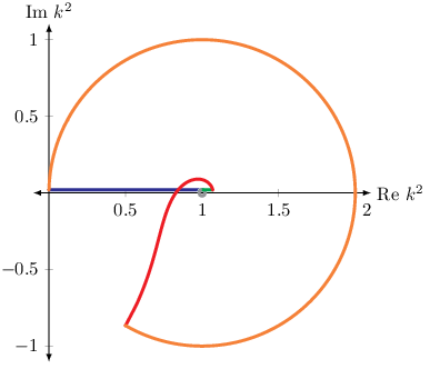
We may now follow this path in k2k^{2}-space.

Refer to caption
Figure 3: The path in k2k^{2}-space. The path wraps in a small circle around the point k2=1k^{2}=1.

The resulting contour is shown in fig. 3. For x=−∞x=-\infty we start with k2=0k^{2}=0. As we increase xx, we continue towards k2=1k^{2}=1. At x=0x=0 the path winds around k2=1k^{2}=1 in a small circle in the clockwise direction [34, 35]. In particular, for k2=1+δk^{2}=1+\delta (with δ\delta infinitesimal) the path crosses the branch cut of the complete elliptic integrals. The contour continues as shown in fig. 3 and crosses the branch cut of the complete elliptic integrals a second time at k2=2k^{2}=2, corresponding to x=16+8​3x=16+8\sqrt{3}. The periods ψisunrise\psi_{i}^{\mathrm{sunrise}} and pseudo-periods ϕisunrise\phi_{i}^{\mathrm{sunrise}} are continuous functions of xx. The matrix γ\gamma in eq. (4) compensates the discontinuity across the branch cut of the complete elliptic integrals and ensures that the periods ψisunrise\psi_{i}^{\mathrm{sunrise}} and pseudo-periods ϕisunrise\phi_{i}^{\mathrm{sunrise}} are continuous. With kk real and k>1k>1 the discontinuities are given by

K⁡(k+i​δ)−K⁡(k−i​δ)\displaystyle K\left(k+i\delta\right)-K\left(k-i\delta\right) =\displaystyle= 2​i​K​(±i​k2−1),\displaystyle 2iK\left(\pm i\sqrt{k^{2}-1}\right),
[K⁡(k+i​δ)−E⁡(k+i​δ)]−[K⁡(k−i​δ)−E⁡(k−i​δ)]\displaystyle\left[K\left(k+i\delta\right)-E\left(k+i\delta\right)\right]-\left[K\left(k-i\delta\right)-E\left(k-i\delta\right)\right] =\displaystyle= 2​i​E​(±i​k2−1).\displaystyle 2iE\left(\pm i\sqrt{k^{2}-1}\right). (79)

We always have Re⁡(k2)>0\mathrm{Re}(k^{2})>0. This implies that the path for k¯2=1−k2\bar{k}^{2}=1-k^{2} never crosses the branch cut of the complete elliptic integrals K⁡(k¯)K(\bar{k}) and E⁡(k¯)E(\bar{k}). Hence, branch cut crossings do not occur for ψ2sunrise\psi_{2}^{\mathrm{sunrise}} and ϕ2sunrise\phi_{2}^{\mathrm{sunrise}}.

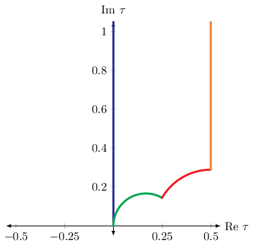
We may then look at the path in τ\tau-space and q¯\bar{q}-space.

Refer to caption
Refer to caption
Figure 4: The path in τ\tau-space and in q¯\bar{q}-space.

This is shown in fig. 4. In the end we will expand in the variable q¯\bar{q} around q¯=0\bar{q}=0. The radius of convergence is determined by the nearest pole, which in our case is located at

q¯=−e−π3​3,\displaystyle\bar{q}=-e^{-\frac{\pi}{3}\sqrt{3}}, (80)

corresponding to x=16x=16. Hence, the expansion converges for

x∈]−∞,−2[\displaystyle x\in\left]-\infty,-2\right[ and x∈]16,∞[.\displaystyle x\in\left]16,\infty\right[. (81)

The value x=−2x=-2 derives from the fact that

|q¯​(x=−2)|=|q¯​(x=16)|=e−π3​3.\displaystyle\left|\bar{q}\left(x=-2\right)\right|\;=\;\left|\bar{q}\left(x=16\right)\right|\;=\;e^{-\frac{\pi}{3}\sqrt{3}}. (82)

5 Modular forms

We introduce a basis {e1,e2}\{e_{1},e_{2}\} for the modular forms of modular weight 11 for the Eisenstein subspace ℰ1​(Γ1​(6)){\mathcal{E}}_{1}(\Gamma_{1}(6)):

e1=E1​(τ,χ1,χ−3),\displaystyle e_{1}\;=\;E_{1}\left(\tau;\chi_{1},\chi_{-3}\right), e2=E1​(2​τ,χ1,χ−3),\displaystyle e_{2}\;=\;E_{1}\left(2\tau;\chi_{1},\chi_{-3}\right), (83)

where

χ1​(n)=(1n)\displaystyle\chi_{1}\left(n\right)\;=\;\left(\frac{1}{n}\right) and χ−3​(n)=(−3n)\displaystyle\chi_{-3}\left(n\right)\;=\;\left(\frac{-3}{n}\right) (84)

denote primitive Dirichlet characters with conductors 11 and 33, respectively. Here, (an)(\frac{a}{n}) denotes the Kronecker symbol in number theory. The generalised Eisenstein series Ek​(τ,χa,χb)E_{k}(\tau;\chi_{a},\chi_{b}) are defined as follows [36], see also [37]: Let χa\chi_{a} and χb\chi_{b} be primitive Dirichlet characters with conductors dad_{a} and dbd_{b}, respectively. Then Ek​(τ,χa,χb)E_{k}(\tau;\chi_{a},\chi_{b}) is defined by

Ek​(τ,χa,χb)\displaystyle E_{k}\left(\tau;\chi_{a},\chi_{b}\right) =a0+∑n=1∞(∑d|nχa​(n/d)⋅χb​(d)⋅dk−1)​q¯n.\displaystyle=a_{0}+\sum\limits_{n=1}^{\infty}\left(\sum\limits_{d|n}\chi_{a}(n/d)\cdot\chi_{b}(d)\cdot d^{k-1}\right)\bar{q}^{n}. (85)

The normalisation is such that the coefficient of q¯\bar{q} is one. The constant term a0a_{0} is given by

a0\displaystyle a_{0} ={−Bk,χb2​k,if​da=1,0,if​da>1.\displaystyle=\begin{cases}-\frac{B_{k,\chi_{b}}}{2k},\qquad&\text{if}\ d_{a}=1,\\ 0,\qquad&\text{if}\ d_{a}>1.\end{cases} (86)

Note that the constant term a0a_{0} depends on χa\chi_{a} and χb\chi_{b}. The generalised Bernoulli numbers Bk,χbB_{k,\chi_{b}} are defined by

∑n=1dbχb​(n)​x​en​xedb​x−1\displaystyle\sum\limits_{n=1}^{d_{b}}\chi_{b}(n)\dfrac{xe^{nx}}{e^{d_{b}x}-1} =\displaystyle= ∑k=0∞Bk,χb​xkk!.\displaystyle\sum\limits_{k=0}^{\infty}B_{k,\chi_{b}}\dfrac{x^{k}}{k!}. (87)

Instead of the basis {e1,e2}\{e_{1},e_{2}\} we may use an alternative basis {b0,b1}\{b_{0},b_{1}\} of ℰ1​(Γ1​(6)){\mathcal{E}}_{1}(\Gamma_{1}(6)). The latter basis is slightly more convenient for the conversion towards modular forms. The basis {b0,b1}\{b_{0},b_{1}\} is defined by

b0=ψ1sunriseπ= 2​3​(e1+e2),\displaystyle b_{0}\;=\;\frac{\psi_{1}^{\mathrm{sunrise}}}{\pi}\;=\;2\sqrt{3}\left(e_{1}+e_{2}\right), b1=y​ψ1sunriseπ= 6​3​(e1−e2).\displaystyle b_{1}\;=\;y\frac{\psi_{1}^{\mathrm{sunrise}}}{\pi}\;=\;6\sqrt{3}\left(e_{1}-e_{2}\right). (88)

An alternative representation of b0b_{0} and b1b_{1} is given as an eta-quotient:

b0=23​3​η​(2​τ)6​η​(3​τ)η​(τ)3​η​(6​τ)2,\displaystyle b_{0}\;=\;\frac{2}{3}\sqrt{3}\frac{\eta\left(2\tau\right)^{6}\eta\left(3\tau\right)}{\eta\left(\tau\right)^{3}\eta\left(6\tau\right)^{2}}, b1= 6​3​η⁡(τ)​η​(6​τ)6η​(2​τ)2​η​(3​τ)3.\displaystyle b_{1}\;=\;6\sqrt{3}\frac{\eta\left(\tau\right)\eta\left(6\tau\right)^{6}}{\eta\left(2\tau\right)^{2}\eta\left(3\tau\right)^{3}}. (89)

Furthermore we may express b0b_{0} and b1b_{1} in terms of the coefficients g(k)​(z,τ)g^{(k)}(z,\tau) of the Kronecker function:

b0=12​π​[g(1)​(13,τ)+g(1)​(16,τ)],\displaystyle b_{0}\;=\;\frac{1}{2\pi}\left[g^{(1)}(\frac{1}{3},\tau)+g^{(1)}(\frac{1}{6},\tau)\right], b1=12​π​[9​g(1)​(13,τ)−3​g(1)​(16,τ)].\displaystyle b_{1}\;=\;\frac{1}{2\pi}\left[9g^{(1)}(\frac{1}{3},\tau)-3g^{(1)}(\frac{1}{6},\tau)\right]. (90)

In addition we introduce two meromorphic modular forms

b3=1(y−3)​ψ1sunriseπ,\displaystyle b_{3}\;=\;\frac{1}{\left(y-3\right)}\frac{\psi_{1}^{\mathrm{sunrise}}}{\pi}, b−3=1(y+3)​ψ1sunriseπ.\displaystyle b_{-3}\;=\;\frac{1}{\left(y+3\right)}\frac{\psi_{1}^{\mathrm{sunrise}}}{\pi}. (91)

We may express all integrands as polynomials in

b0,b1,b3,b−3.\displaystyle b_{0},\;\;\;b_{1},\;\;\;b_{3},\;\;\;b_{-3}. (92)

For example, the meromorphic modular form g6g_{6} of eq. (45) is expressed as

g6\displaystyle g_{6} =\displaystyle= 1864​b0​b15−11144​b02​b14+10754​b03​b13−42116​b04​b12+668532​b05​b1−1251​b06+108​b03​b33\displaystyle\frac{1}{864}b_{0}b_{1}^{5}-\frac{11}{144}b_{0}^{2}b_{1}^{4}+\frac{107}{54}b_{0}^{3}b_{1}^{3}-\frac{421}{16}b_{0}^{4}b_{1}^{2}+\frac{6685}{32}b_{0}^{5}b_{1}-1251b_{0}^{6}+108b_{0}^{3}b_{3}^{3} (93)
+162​b04​b32+81​b05​b3+6912​b03​b−33−10368​b04​b−32+6480​b05​b−3.\displaystyle+162b_{0}^{4}b_{3}^{2}+81b_{0}^{5}b_{3}+6912b_{0}^{3}b_{-3}^{3}-10368b_{0}^{4}b_{-3}^{2}+6480b_{0}^{5}b_{-3}.

The q¯\bar{q}-expansions of the four basic modular forms b0b_{0}, b1b_{1}, b3b_{3} and b−3b_{-3} start as

b0\displaystyle b_{0} =\displaystyle= 2​3​[13+q¯+q¯2+q¯3+q¯4]+𝒪⁡(q¯6),\displaystyle 2\sqrt{3}\left[\frac{1}{3}+\bar{q}+\bar{q}^{2}+\bar{q}^{3}+\bar{q}^{4}\right]+{\mathcal{O}}\left(\bar{q}^{6}\right),
b1\displaystyle b_{1} =\displaystyle= 6​3​[q¯−q¯2+q¯3+q¯4]+𝒪⁡(q¯6),\displaystyle 6\sqrt{3}\left[\bar{q}-\bar{q}^{2}+\bar{q}^{3}+\bar{q}^{4}\right]+{\mathcal{O}}\left(\bar{q}^{6}\right),
b3\displaystyle b_{3} =\displaystyle= −43​3​[16+q¯+32​q¯2−2​q¯3−72​q¯4+18​q¯5]+𝒪⁡(q¯6),\displaystyle-\frac{4}{3}\sqrt{3}\left[\frac{1}{6}+\bar{q}+\frac{3}{2}\bar{q}^{2}-2\bar{q}^{3}-\frac{7}{2}\bar{q}^{4}+18\bar{q}^{5}\right]+{\mathcal{O}}\left(\bar{q}^{6}\right),
b−3\displaystyle b_{-3} =\displaystyle= 29​3​[1+15​q¯2−72​q¯3+459​q¯4−2808​q¯5]+𝒪⁡(q¯6).\displaystyle\frac{2}{9}\sqrt{3}\left[1+15\bar{q}^{2}-72\bar{q}^{3}+459\bar{q}^{4}-2808\bar{q}^{5}\right]+{\mathcal{O}}\left(\bar{q}^{6}\right). (94)

We then have for example

g6\displaystyle g_{6} =\displaystyle= −2​q¯+104​q¯2−2286​q¯3+30112​q¯4−306300​q¯5+𝒪⁡(q¯6).\displaystyle-2\bar{q}+104\bar{q}^{2}-2286\bar{q}^{3}+30112\bar{q}^{4}-306300\bar{q}^{5}+{\mathcal{O}}\left(\bar{q}^{6}\right). (95)

The modular form g6g_{6} is rather special: We have verified to very high order (𝒪⁡(q¯200){\mathcal{O}}(\bar{q}^{200})) that all coefficients are integers and that the coefficient of q¯n\bar{q}^{n} is divisible by n2n^{2}.

6 Iterated integrals of modular forms

Let f1​(τ)f_{1}(\tau), f2​(τ)f_{2}(\tau), …, fn​(τ)f_{n}(\tau) be a set of (meromorphic) modular forms. We define the nn-fold iterated integral of these modular forms by

I⁡(f1,f2,…,fn,τ,τ0)\displaystyle I\left(f_{1},f_{2},...,f_{n};\tau,\tau_{0}\right) =(2​π​i)n​∫τ0τd​τ1​∫τ0τ1d​τ2​…​∫τ0τn−1d​τn​f1​(τ1)​f2​(τ2)​…​fn​(τn).\displaystyle=\left(2\pi i\right)^{n}\int\limits_{\tau_{0}}^{\tau}d\tau_{1}\int\limits_{\tau_{0}}^{\tau_{1}}d\tau_{2}...\int\limits_{\tau_{0}}^{\tau_{n-1}}d\tau_{n}\;f_{1}\left(\tau_{1}\right)f_{2}\left(\tau_{2}\right)...f_{n}\left(\tau_{n}\right). (96)

With q¯=exp⁡(2​π​i​τ)\bar{q}=\exp(2\pi i\tau) we may equally well write

I⁡(f1,f2,…,fn,τ,τ0)\displaystyle I\left(f_{1},f_{2},...,f_{n};\tau,\tau_{0}\right) =∫q¯0q¯d​q¯1q¯1​∫q¯0q¯1d​q¯2q¯2​…​∫q¯0q¯n−1d​q¯nq¯n​f1​(τ1)​f2​(τ2)​…​fn​(τn),τj=12​π​i​ln⁡q¯j.\displaystyle=\int\limits_{\bar{q}_{0}}^{\bar{q}}\frac{d\bar{q}_{1}}{\bar{q}_{1}}\int\limits_{\bar{q}_{0}}^{\bar{q}_{1}}\frac{d\bar{q}_{2}}{\bar{q}_{2}}...\int\limits_{\bar{q}_{0}}^{\bar{q}_{n-1}}\frac{d\bar{q}_{n}}{\bar{q}_{n}}\;f_{1}\left(\tau_{1}\right)f_{2}\left(\tau_{2}\right)...f_{n}\left(\tau_{n}\right),\qquad\tau_{j}=\frac{1}{2\pi i}\ln\bar{q}_{j}. (97)

Our standard choice for the base point τ0\tau_{0} will be τ0=i​∞\tau_{0}=i\infty, corresponding to q0=0q_{0}=0. If fn​(τ)f_{n}(\tau) does not vanish at the cusp τ=i​∞\tau=i\infty we employ the standard “trailing zero” or “tangential base point” regularisation [38, 25, 39]: We first take q¯0\bar{q}_{0} to have a small non-zero value. The integration will produce terms with ln⁡(q¯0)\ln(\bar{q}_{0}). Let RR be the operator, which removes all ln⁡(q¯0)\ln(\bar{q}_{0})-terms. After these terms have been removed, we may take the limit q¯0→0\bar{q}_{0}\rightarrow 0. With this regularisation we set

I⁡(f1,f2,…,fn,τ)\displaystyle I\left(f_{1},f_{2},...,f_{n};\tau\right) =limq¯0→0R⁡[∫q¯0q¯d​q¯1q¯1​∫q¯0q¯1d​q¯2q¯2​…​∫q¯0q¯n−1d​q¯nq¯n​f1​(τ1)​f2​(τ2)​…​fn​(τn)].\displaystyle=\lim\limits_{\bar{q}_{0}\rightarrow 0}R\left[\int\limits_{\bar{q}_{0}}^{\bar{q}}\frac{d\bar{q}_{1}}{\bar{q}_{1}}\int\limits_{\bar{q}_{0}}^{\bar{q}_{1}}\frac{d\bar{q}_{2}}{\bar{q}_{2}}...\int\limits_{\bar{q}_{0}}^{\bar{q}_{n-1}}\frac{d\bar{q}_{n}}{\bar{q}_{n}}\;f_{1}\left(\tau_{1}\right)f_{2}\left(\tau_{2}\right)...f_{n}\left(\tau_{n}\right)\right]. (98)

In this notation the expression F2F_{2} from eq. (44) becomes

F2\displaystyle F_{2} =\displaystyle= I⁡(1,g6,τ).\displaystyle I\left(1,g_{6};\tau\right). (99)

Furthermore it will be convenient to introduce a short-hand notation for repeated letters. We use the notation

{fi}j\displaystyle\left\{f_{i}\right\}^{j} =fi,fi,…,fi⏟j\displaystyle=\underbrace{f_{i},f_{i},...,f_{i}}_{j} (100)

to denote a sequence of jj letters fif_{i}. For iterated integrals we have the shuffle product, for example

I⁡(f1,f2,τ)​I​(f3,τ)\displaystyle I\left(f_{1},f_{2};\tau\right)I\left(f_{3};\tau\right) =\displaystyle= I⁡(f1,f2,f3,τ)+I⁡(f1,f3,f2,τ)+I⁡(f3,f1,f2,τ).\displaystyle I\left(f_{1},f_{2},f_{3};\tau\right)+I\left(f_{1},f_{3},f_{2};\tau\right)+I\left(f_{3},f_{1},f_{2};\tau\right). (101)

Using the antipode in the shuffle algebra [37] one easily shows that

I⁡(fk,{1}j,τ)\displaystyle I\left(f_{k},\left\{1\right\}^{j};\tau\right) =\displaystyle= ∑i=0j(−1)i​I​({1}j−i,τ)​I​({1}i,fk,τ),\displaystyle\sum\limits_{i=0}^{j}\left(-1\right)^{i}I\left(\left\{1\right\}^{j-i};\tau\right)I\left(\left\{1\right\}^{i},f_{k};\tau\right),
I⁡({1}j,fk,τ)\displaystyle I\left(\left\{1\right\}^{j},f_{k};\tau\right) =\displaystyle= ∑i=0j(−1)i​I​({1}j−i,τ)​I​(fk,{1}i,τ).\displaystyle\sum\limits_{i=0}^{j}\left(-1\right)^{i}I\left(\left\{1\right\}^{j-i};\tau\right)I\left(f_{k},\left\{1\right\}^{i};\tau\right). (102)

These relations will be useful when we work out the modular transformation properties of F2F_{2}.

7 The differential equation

For the basis II the differential equation is in ε\varepsilon-form

d​I\displaystyle dI =\displaystyle= ε​A​I,\displaystyle\varepsilon AI, (103)

with

A\displaystyle A =\displaystyle= 2​π​i​(00000−f2,a−f2,b100f4,b−f2,a+2​f2,b1f4,af6f4,b−f2,a−f2,b)​d​τ.\displaystyle 2\pi i\left(\begin{array}[]{cccc}0&0&0&0\\ 0&-f_{2,a}-f_{2,b}&1&0\\ 0&f_{4,b}&-f_{2,a}+2f_{2,b}&1\\ f_{4,a}&f_{6}&f_{4,b}&-f_{2,a}-f_{2,b}\\ \end{array}\right)d\tau.

This is a differential equation with an alphabet consisting of six letters

𝒜\displaystyle{\mathcal{A}} =\displaystyle= {1,f2,a,f2,b,f4,a,f4,b,f6}.\displaystyle\left\{1,f_{2,a},f_{2,b},f_{4,a},f_{4,b},f_{6}\right\}. (109)

Below we give expressions for all non-trivial letters in xx-space, yy-space and τ\tau-space.

The differential one-forms f2,af_{2,a} and f2,bf_{2,b} are of modular weight 22. The meromorphic modular form f2,af_{2,a} is just the translation of a dlog-form to the variable τ\tau:

f2,a⋅2​π​i​d​τ\displaystyle f_{2,a}\cdot 2\pi id\tau =\displaystyle= d​ln⁡(x−4)+d​ln⁡(x−16).\displaystyle d\ln\left(x-4\right)+d\ln\left(x-16\right). (110)

We have

f2,a\displaystyle f_{2,a} =\displaystyle= (1x−4+1x−16)​ψ122​π​i​W\displaystyle\left(\frac{1}{x-4}+\frac{1}{x-16}\right)\frac{\psi_{1}^{2}}{2\pi iW} (111)
=\displaystyle= [16​y2−53​y+92−6y−3−24y+3]​(ψ1sunriseπ)2\displaystyle\left[\frac{1}{6}y^{2}-\frac{5}{3}y+\frac{9}{2}-\frac{6}{y-3}-\frac{24}{y+3}\right]\left(\frac{\psi_{1}^{\mathrm{sunrise}}}{\pi}\right)^{2}
=\displaystyle= 16​b12−53​b0​b1+92​b02−6​b0​b3−24​b0​b−3.\displaystyle\frac{1}{6}b_{1}^{2}-\frac{5}{3}b_{0}b_{1}+\frac{9}{2}b_{0}^{2}-6b_{0}b_{3}-24b_{0}b_{-3}.

The differential one-form f2,bf_{2,b} is given by

f2,b\displaystyle f_{2,b} =\displaystyle= F2,\displaystyle F_{2}, (112)

with

F2\displaystyle F_{2} =\displaystyle= I⁡(1,g6,τ)\displaystyle I\left(1,g_{6};\tau\right) (113)

and

g6\displaystyle g_{6} =\displaystyle= x⁡(x−8)​(x+8)3864​(4−x)32​(16−x)32​(ψ1π)6\displaystyle\frac{x\left(x-8\right)\left(x+8\right)^{3}}{864\left(4-x\right)^{\frac{3}{2}}\left(16-x\right)^{\frac{3}{2}}}\left(\frac{\psi_{1}}{\pi}\right)^{6} (114)
=\displaystyle= y⁡(y−1)​(y−9)​(y2−2​y+9)​(y2−18​y+9)3864​(y−3)3​(y+3)3​(ψ1sunriseπ)6\displaystyle\frac{y\left(y-1\right)\left(y-9\right)\left(y^{2}-2y+9\right)\left(y^{2}-18y+9\right)^{3}}{864\left(y-3\right)^{3}\left(y+3\right)^{3}}\left(\frac{\psi_{1}^{\mathrm{sunrise}}}{\pi}\right)^{6}
=\displaystyle= 1864​b0​b15−11144​b02​b14+10754​b03​b13−42116​b04​b12+668532​b05​b1−1251​b06+108​b03​b33\displaystyle\frac{1}{864}b_{0}b_{1}^{5}-\frac{11}{144}b_{0}^{2}b_{1}^{4}+\frac{107}{54}b_{0}^{3}b_{1}^{3}-\frac{421}{16}b_{0}^{4}b_{1}^{2}+\frac{6685}{32}b_{0}^{5}b_{1}-1251b_{0}^{6}+108b_{0}^{3}b_{3}^{3}
+162​b04​b32+81​b05​b3+6912​b03​b−33−10368​b04​b−32+6480​b05​b−3.\displaystyle+162b_{0}^{4}b_{3}^{2}+81b_{0}^{5}b_{3}+6912b_{0}^{3}b_{-3}^{3}-10368b_{0}^{4}b_{-3}^{2}+6480b_{0}^{5}b_{-3}.

f4,af_{4,a} and f4,bf_{4,b} are of modular weight 44. The differential one-form f4,af_{4,a} is a (holomorphic) modular form and given by

f4,a\displaystyle f_{4,a} =\displaystyle= 172​x​(4−x)12​(16−x)12​(ψ1π)4\displaystyle\frac{1}{72}x\left(4-x\right)^{\frac{1}{2}}\left(16-x\right)^{\frac{1}{2}}\left(\frac{\psi_{1}}{\pi}\right)^{4} (115)
=\displaystyle= 172​(y−1)​(y−9)​(y−3)​(y+3)​(ψ1sunriseπ)4\displaystyle\frac{1}{72}\left(y-1\right)\left(y-9\right)\left(y-3\right)\left(y+3\right)\left(\frac{\psi_{1}^{\mathrm{sunrise}}}{\pi}\right)^{4}
=\displaystyle= 172​b14−536​b0​b13+54​b03​b1−98​b04.\displaystyle\frac{1}{72}b_{1}^{4}-\frac{5}{36}b_{0}b_{1}^{3}+\frac{5}{4}b_{0}^{3}b_{1}-\frac{9}{8}b_{0}^{4}.

The differential one-form f4,bf_{4,b} is given by

f4,b\displaystyle f_{4,b} =\displaystyle= (x+8)2​(x2−8​x+64)288​(x−4)​(x−16)​(ψ1π)4−32​F22\displaystyle\frac{\left(x+8\right)^{2}\left(x^{2}-8x+64\right)}{288\left(x-4\right)\left(x-16\right)}\left(\frac{\psi_{1}}{\pi}\right)^{4}-\frac{3}{2}F_{2}^{2} (116)
=\displaystyle= (y2−18​y+9)2​(y4−12​y3+102​y2−108​y+81)288​(y−3)2​(y+3)2​(ψ1sunriseπ)4−32​F22\displaystyle\frac{\left(y^{2}-18y+9\right)^{2}\left(y^{4}-12y^{3}+102y^{2}-108y+81\right)}{288\left(y-3\right)^{2}\left(y+3\right)^{2}}\left(\frac{\psi_{1}^{\mathrm{sunrise}}}{\pi}\right)^{4}-\frac{3}{2}F_{2}^{2}
=\displaystyle= 1288​b14−16​b0​b13+14948​b02​b12−632​b03​b1+653732​b04+54​b02​b32+54​b03​b3\displaystyle\frac{1}{288}b_{1}^{4}-\frac{1}{6}b_{0}b_{1}^{3}+\frac{149}{48}b_{0}^{2}b_{1}^{2}-\frac{63}{2}b_{0}^{3}b_{1}+\frac{6537}{32}b_{0}^{4}+54b_{0}^{2}b_{3}^{2}+54b_{0}^{3}b_{3}
+864​b02​b−32−864​b03​b−3−32​F22.\displaystyle+864b_{0}^{2}b_{-3}^{2}-864b_{0}^{3}b_{-3}-\frac{3}{2}F_{2}^{2}.

Finally, at modular weight 66 we have

f6\displaystyle f_{6} =\displaystyle= x⁡(x−8)​(x+8)3216​(4−x)32​(16−x)32​(ψ1π)6−(x+8)2​(x2−8​x+64)144​(x−4)​(x−16)​(ψ1π)4​F2+F23\displaystyle\frac{x\left(x-8\right)\left(x+8\right)^{3}}{216\left(4-x\right)^{\frac{3}{2}}\left(16-x\right)^{\frac{3}{2}}}\left(\frac{\psi_{1}}{\pi}\right)^{6}-\frac{\left(x+8\right)^{2}\left(x^{2}-8x+64\right)}{144\left(x-4\right)\left(x-16\right)}\left(\frac{\psi_{1}}{\pi}\right)^{4}F_{2}+F_{2}^{3} (117)
=\displaystyle= y⁡(y−1)​(y−9)​(y2−2​y+9)​(y2−18​y+9)3216​(y−3)3​(y+3)3​(ψ1sunriseπ)6\displaystyle\frac{y\left(y-1\right)\left(y-9\right)\left(y^{2}-2y+9\right)\left(y^{2}-18y+9\right)^{3}}{216\left(y-3\right)^{3}\left(y+3\right)^{3}}\left(\frac{\psi_{1}^{\mathrm{sunrise}}}{\pi}\right)^{6}
−(y2−18​y+9)2​(y4−12​y3+102​y2−108​y+81)144​(y−3)2​(y+3)2​(ψ1sunriseπ)4​F2+F23\displaystyle-\frac{\left(y^{2}-18y+9\right)^{2}\left(y^{4}-12y^{3}+102y^{2}-108y+81\right)}{144\left(y-3\right)^{2}\left(y+3\right)^{2}}\left(\frac{\psi_{1}^{\mathrm{sunrise}}}{\pi}\right)^{4}F_{2}+F_{2}^{3}
=\displaystyle= 1216​b0​b15−1136​b02​b14+21427​b03​b13−4214​b04​b12+66858​b05​b1−5004​b06+432​b03​b33\displaystyle\frac{1}{216}b_{0}b_{1}^{5}-\frac{11}{36}b_{0}^{2}b_{1}^{4}+\frac{214}{27}b_{0}^{3}b_{1}^{3}-\frac{421}{4}b_{0}^{4}b_{1}^{2}+\frac{6685}{8}b_{0}^{5}b_{1}-5004b_{0}^{6}+432b_{0}^{3}b_{3}^{3}
+648b04b32+324b05b3+27648b03b−33−41472b04b−32+25920b05b−3−[1144b14−13b0b13\displaystyle+648b_{0}^{4}b_{3}^{2}+324b_{0}^{5}b_{3}+27648b_{0}^{3}b_{-3}^{3}-41472b_{0}^{4}b_{-3}^{2}+25920b_{0}^{5}b_{-3}-\left[\frac{1}{144}b_{1}^{4}-\frac{1}{3}b_{0}b_{1}^{3}\right.
+14924b02b12−63b03b1+653716b04+108b02b32+108b03b3+1728b02b−32−1728b03b−3]F2\displaystyle\left.+\frac{149}{24}b_{0}^{2}b_{1}^{2}-63b_{0}^{3}b_{1}+\frac{6537}{16}b_{0}^{4}+108b_{0}^{2}b_{3}^{2}+108b_{0}^{3}b_{3}+1728b_{0}^{2}b_{-3}^{2}-1728b_{0}^{3}b_{-3}\right]F_{2}
+F23.\displaystyle+F_{2}^{3}.

With the help of eq. (76) and eq. (88) the q¯\bar{q}-expansions of f2,af_{2,a}, f2,bf_{2,b}, f4,af_{4,a}, f4,bf_{4,b} and f6f_{6} are readily obtained. The first few terms read

f2,a\displaystyle f_{2,a} =\displaystyle= −2+8​q¯−44​q¯2+440​q¯3−2956​q¯4+17328​q¯5+𝒪⁡(q¯6),\displaystyle-2+8\bar{q}-44\bar{q}^{2}+440\bar{q}^{3}-2956\bar{q}^{4}+17328\bar{q}^{5}+{\mathcal{O}}\left(\bar{q}^{6}\right),
f2,b\displaystyle f_{2,b} =\displaystyle= −2​q¯+26​q¯2−254​q¯3+1882​q¯4−12252​q¯5+𝒪⁡(q¯6),\displaystyle-2\bar{q}+26\bar{q}^{2}-254\bar{q}^{3}+1882\bar{q}^{4}-12252\bar{q}^{5}+{\mathcal{O}}\left(\bar{q}^{6}\right),
f4,a\displaystyle f_{4,a} =\displaystyle= −2−4​q¯+28​q¯2−76​q¯3+284​q¯4−504​q¯5+𝒪⁡(q¯6),\displaystyle-2-4\bar{q}+28\bar{q}^{2}-76\bar{q}^{3}+284\bar{q}^{4}-504\bar{q}^{5}+{\mathcal{O}}\left(\bar{q}^{6}\right),
f4,b\displaystyle f_{4,b} =\displaystyle= 12−18​q¯+282​q¯2−3150​q¯3+28314​q¯4−200268​q¯5+𝒪⁡(q¯6),\displaystyle\frac{1}{2}-18\bar{q}+282\bar{q}^{2}-3150\bar{q}^{3}+28314\bar{q}^{4}-200268\bar{q}^{5}+{\mathcal{O}}\left(\bar{q}^{6}\right),
f6\displaystyle f_{6} =\displaystyle= −6​q¯+318​q¯2−6810​q¯3+81534​q¯4−710676​q¯5+𝒪⁡(q¯6).\displaystyle-6\bar{q}+318\bar{q}^{2}-6810\bar{q}^{3}+81534\bar{q}^{4}-710676\bar{q}^{5}+{\mathcal{O}}\left(\bar{q}^{6}\right). (118)

We have checked to very high order (𝒪⁡(q¯200){\mathcal{O}}(\bar{q}^{200})) that with the exception of the constant term of f4,bf_{4,b} all coefficients are integers.

Let us now look at the poles at x=4x=4 and x=16x=16 in τ\tau-space. The Jacobian for the transformation from τ\tau-space to yy-space is smooth in a neighbourhood of these points, so we may discuss the poles in yy-space. From eq. (114) we see that g6g_{6} has a triple pole at y=3y=3 (corresponding to x=4x=4) and at y=−3y=-3 (corresponding to x=16x=16). However, f2,bf_{2,b} has only a simple pole at y=±3y=\pm 3. For f4,bf_{4,b} and f6f_{6}, the triple and double poles appearing in the individual terms of their definition cancel in the sum, leaving f4,bf_{4,b} and f6f_{6} with a simple pole at y=±3y=\pm 3. In summary it follows that all entries of the differential equation have at most a simple pole at y=±3y=\pm 3.

8 Modular transformations

In this section we discuss the behaviour of f2,af_{2,a}, f2,bf_{2,b}, f4,af_{4,a}, f4,bf_{4,b} and f6f_{6} under modular transformations. We start with a few definitions. Let

γ\displaystyle\gamma =\displaystyle= (abcd)∈Γ.\displaystyle\left(\begin{array}[]{cc}a&b\\ c&d\\ \end{array}\right)\;\in\;\Gamma.

We consider the transformation

τ′=γ⁡(τ)=a​τ+bc​τ+d,\displaystyle\tau^{\prime}\;=\;\gamma\left(\tau\right)\;=\;\frac{a\tau+b}{c\tau+d}, d​τ′=d​τ(c​τ+d)2.\displaystyle d\tau^{\prime}\;=\;\frac{d\tau}{\left(c\tau+d\right)^{2}}. (122)

The point τ′=ac\tau^{\prime}=\frac{a}{c} corresponds to τ=i​∞\tau=i\infty.

Let f:ℍ→ℂ^f:{\mathbb{H}}\rightarrow\hat{{\mathbb{C}}} be a function from the complex upper half-plane to ℂ^=ℂ∪{∞}\hat{{\mathbb{C}}}={\mathbb{C}}\cup\{\infty\}. We define

(f|k​γ)​(τ)\displaystyle(f|_{k}\gamma)(\tau) =\displaystyle= (c​τ+d)−k⋅f⁡(γ⁡(τ)).\displaystyle(c\tau+d)^{-k}\cdot f(\gamma(\tau)). (123)

We say that ff transforms as a modular form of modular weight kk (or is weakly modular) if

(f|k​γ)​(τ)\displaystyle(f|_{k}\gamma)(\tau) =\displaystyle= f⁡(τ).\displaystyle f(\tau). (124)

We say that ff transforms as a quasi-modular form of modular weight kk and depth pp if there are f1,…,fpf_{1},\dots,f_{p} such that

(f|k​γ)​(τ)\displaystyle(f|_{k}\gamma)(\tau) =\displaystyle= f⁡(τ)+∑j=1p(cc​τ+d)j​fj​(τ).\displaystyle f(\tau)+\sum\limits_{j=1}^{p}\left(\frac{c}{c\tau+d}\right)^{j}f_{j}(\tau). (125)

We need one more generalisation: We say that ff transforms as “quasi-Eichler” of modular weight kk and depth pp if

(f|k​γ)​(τ)\displaystyle(f|_{k}\gamma)(\tau) =\displaystyle= f⁡(τ)+∑j=1p(cc​τ+d)j​fj​(τ)+Pγ​(τ)(c​τ+d)p,\displaystyle f(\tau)+\sum\limits_{j=1}^{p}\left(\frac{c}{c\tau+d}\right)^{j}f_{j}(\tau)+\frac{P_{\gamma}(\tau)}{\left(c\tau+d\right)^{p}}, (126)

where Pγ​(τ)P_{\gamma}(\tau) is a polynomial in τ\tau of degree at most (p−k)(p-k). Note that the fjf_{j}’s are independent of γ\gamma, while the polynomial PγP_{\gamma} may depend on γ\gamma. A special case is an Eichler integral, which corresponds to the case p=0p=0: ff transforms as an Eichler integral of modular weight kk (with k<0k<0) if there is a polynomial Pγ​(τ)P_{\gamma}(\tau) of degree at most (−k)(-k) such that

(f|k​γ)​(τ)\displaystyle(f|_{k}\gamma)(\tau) =\displaystyle= f​(τ)+Pγ​(τ).\displaystyle f(\tau)+P_{\gamma}(\tau). (127)

We now specialise to Γ=Γ1​(6)\Gamma=\Gamma_{1}(6). Generators of Γ1​(6)\Gamma_{1}(6) are

{(1101),(−51−61),(7−312−5)}.\displaystyle\left\{\left(\begin{array}[]{rr}1&1\\ 0&1\\ \end{array}\right),\left(\begin{array}[]{rr}-5&1\\ -6&1\\ \end{array}\right),\left(\begin{array}[]{rr}7&-3\\ 12&-5\\ \end{array}\right)\right\}.

f4,af_{4,a} is a (holomorphic) modular form for Γ1​(6)\Gamma_{1}(6), f2,af_{2,a} is a meromorphic modular form for Γ1​(6)\Gamma_{1}(6). Both transform for γ∈Γ1​(6)\gamma\in\Gamma_{1}(6) according to eq. (124).

We work out the behaviour of f2,bf_{2,b} under modular transformations. We start from

f2,b​(τ′)\displaystyle f_{2,b}\left(\tau^{\prime}\right) =\displaystyle= I⁡(1,g6,i​∞,τ′).\displaystyle I\left(1,g_{6};i\infty,\tau^{\prime}\right). (135)

The path composition formula for iterated integrals gives us

f2,b​(τ′)\displaystyle f_{2,b}\left(\tau^{\prime}\right) =\displaystyle= I⁡(1,g6,ac,τ′)+I⁡(g6,i​∞,ac)​I​(1,ac,τ′)+I⁡(1,g6,i​∞,ac).\displaystyle I\left(1,g_{6};\frac{a}{c},\tau^{\prime}\right)+I\left(g_{6};i\infty,\frac{a}{c}\right)I\left(1;\frac{a}{c},\tau^{\prime}\right)+I\left(1,g_{6};i\infty,\frac{a}{c}\right). (136)

Let us emphasise that we require the combined path in τ′\tau^{\prime}-space, consisting of the path from i​∞i\infty to a/ca/c followed by the path from a/ca/c to τ′\tau^{\prime} followed by the reverse path from τ′\tau^{\prime} to i​∞i\infty to be homotopy equivalent to the zero path (i.e. no poles are encircled and no branch cuts are crossed). We define two constants

C6=I⁡(g6,i​∞,ac),\displaystyle C_{6}\;=\;I\left(g_{6};i\infty,\frac{a}{c}\right), C1,6=I⁡(1,g6,i​∞,ac).\displaystyle C_{1,6}\;=\;I\left(1,g_{6};i\infty,\frac{a}{c}\right). (137)

Furthermore we have

I⁡(1,ac,τ′)\displaystyle I\left(1;\frac{a}{c},\tau^{\prime}\right) =\displaystyle= 2​π​i​(τ′−ac)=−2​π​ic​(c​τ+d)−1.\displaystyle 2\pi i\left(\tau^{\prime}-\frac{a}{c}\right)\;=\;-\frac{2\pi i}{c}\left(c\tau+d\right)^{-1}. (138)

A leading one will introduce a negative power of the automorphic factor (c​τ+d)(c\tau+d) in the integrand. This can be avoided by first using eq. (6) to convert any leading 11’s to trailing 11’s, using then the modular transformation law for the integrands and in the end converting back to leading 11’s, again with the help of eq. (6). We find

(f2,b|2​γ)​(τ)\displaystyle(f_{2,b}|_{2}\gamma)(\tau) =\displaystyle= f2,b​(τ)−6​cc​τ+d​12​π​i​I​(1,1,g6,τ)+18​(cc​τ+d)2​1(2​π​i)2​I​(1,1,1,g6,τ)\displaystyle f_{2,b}(\tau)-6\frac{c}{c\tau+d}\frac{1}{2\pi i}I\left(1,1,g_{6};\tau\right)+18\left(\frac{c}{c\tau+d}\right)^{2}\frac{1}{\left(2\pi i\right)^{2}}I\left(1,1,1,g_{6};\tau\right) (139)
−24​(cc​τ+d)3​1(2​π​i)3​I​(1,1,1,1,g6,τ)+C1,6(c​τ+d)2−2​π​i​C6c​(c​τ+d)3.\displaystyle-24\left(\frac{c}{c\tau+d}\right)^{3}\frac{1}{\left(2\pi i\right)^{3}}I\left(1,1,1,1,g_{6};\tau\right)+\frac{C_{1,6}}{\left(c\tau+d\right)^{2}}-\frac{2\pi iC_{6}}{c\left(c\tau+d\right)^{3}}.

We see that f2,bf_{2,b} transforms as quasi-Eichler of modular weight 22 and depth 33.

Once the transformation law for F2=f2,bF_{2}=f_{2,b} under modular transformations γ∈Γ1​(6)\gamma\in\Gamma_{1}(6) is known, the transformation laws for f4,bf_{4,b} and f6f_{6} follow from the definition of these quantities. They are given as polynomials of building blocks, whose transformation is known.

9 Analytical results

We write for the ε\varepsilon-expansion of the master integrals

Ij\displaystyle I_{j} =\displaystyle= ∑k=0∞Ij(k)​εk.\displaystyle\sum\limits_{k=0}^{\infty}I_{j}^{(k)}\varepsilon^{k}. (140)

Up to order ε4\varepsilon^{4} the results are still relatively compact and we list them below. Results up to order ε6\varepsilon^{6} can be found in an ancillary file attached to this article. The master integral I1I_{1} is very simple and given by

I1\displaystyle I_{1} =\displaystyle= 1+32​ζ2​ε2−ζ3​ε3+5716​ζ4​ε4+𝒪⁡(ε5).\displaystyle 1+\frac{3}{2}\zeta_{2}\varepsilon^{2}-\zeta_{3}\varepsilon^{3}+\frac{57}{16}\zeta_{4}\varepsilon^{4}+{\mathcal{O}}\left(\varepsilon^{5}\right). (141)

The interesting master integrals are I2I_{2}, I3I_{3} and I4I_{4}. The master integral I2I_{2} starts at order ε3\varepsilon^{3}. Its terms of order ε3\varepsilon^{3} and ε4\varepsilon^{4} are given by

I2(3)\displaystyle I_{2}^{(3)} =\displaystyle= 43​ζ3+I⁡(1,1,f4,a,τ),\displaystyle\frac{4}{3}\zeta_{3}+I\left(1,1,f_{4,a};\tau\right),
I2(4)\displaystyle I_{2}^{(4)} =\displaystyle= 2​ζ4+43​ζ3​[112​ln⁡(q¯)−I⁡(f2,a,τ)−I⁡(f2,b,τ)]+ζ2​ln2⁡(q¯)−I⁡(1,1,f2,a,f4,a,τ)\displaystyle 2\zeta_{4}+\frac{4}{3}\zeta_{3}\left[\frac{11}{2}\ln\left(\bar{q}\right)-I\left(f_{2,a};\tau\right)-I\left(f_{2,b};\tau\right)\right]+\zeta_{2}\ln^{2}\left(\bar{q}\right)-I\left(1,1,f_{2,a},f_{4,a};\tau\right) (142)
−I⁡(1,f2,a,1,f4,a,τ)−I⁡(f2,a,1,1,f4,a,τ)−I⁡(1,1,f2,b,f4,a,τ)\displaystyle-I\left(1,f_{2,a},1,f_{4,a};\tau\right)-I\left(f_{2,a},1,1,f_{4,a};\tau\right)-I\left(1,1,f_{2,b},f_{4,a};\tau\right)
+2​I​(1,f2,b,1,f4,a,τ)−I⁡(f2,b,1,1,f4,a,τ).\displaystyle+2I\left(1,f_{2,b},1,f_{4,a};\tau\right)-I\left(f_{2,b},1,1,f_{4,a};\tau\right).

The term I2(3)I_{2}^{(3)} agrees with the result of Bloch, Kerr and Vanhove [17]. In our notation their result reads

I2(3)\displaystyle I_{2}^{(3)} =\displaystyle= 43​ζ3−13​ln3⁡(q¯)−4​∑n=1∞χ⁡(n)n3​q¯n1−q¯n,\displaystyle\frac{4}{3}\zeta_{3}-\frac{1}{3}\ln^{3}\left(\bar{q}\right)-4\sum\limits_{n=1}^{\infty}\frac{\chi\left(n\right)}{n^{3}}\frac{\bar{q}^{n}}{1-\bar{q}^{n}}, (143)

where χ\chi is a character of modulus six (i.e. χ⁡(n+6)=χ⁡(n)\chi(n+6)=\chi(n)), taking the values

n012345χ1201−15−8−151.\displaystyle\begin{array}[]{c|rrrrrr}n&0&1&2&3&4&5\\ \hline\cr\chi&120&1&-15&-8&-15&1\\ \end{array}.

The master integral I3I_{3} starts at order ε2\varepsilon^{2}. The non-zero terms up to order ε4\varepsilon^{4} read

I3(2)\displaystyle I_{3}^{(2)} =\displaystyle= I⁡(1,f4,a,τ),\displaystyle I\left(1,f_{4,a};\tau\right),
I3(3)\displaystyle I_{3}^{(3)} =\displaystyle= 223​ζ3+2​ζ2​ln⁡(q¯)−I⁡(1,f2,a,f4,a,τ)−I⁡(f2,a,1,f4,a,τ)−I⁡(1,f2,b,f4,a,τ)\displaystyle\frac{22}{3}\zeta_{3}+2\zeta_{2}\ln\left(\bar{q}\right)-I\left(1,f_{2,a},f_{4,a};\tau\right)-I\left(f_{2,a},1,f_{4,a};\tau\right)-I\left(1,f_{2,b},f_{4,a};\tau\right)
+2​I​(f2,b,1,f4,a,τ),\displaystyle+2I\left(f_{2,b},1,f_{4,a};\tau\right),
I3(4)\displaystyle I_{3}^{(4)} =\displaystyle= 172​ζ4+43​ζ3​[8​ln⁡(q¯)−112​I​(f2,a,τ)+11​I​(f2,b,τ)+I⁡(f4,b,τ)]\displaystyle\frac{17}{2}\zeta_{4}+\frac{4}{3}\zeta_{3}\left[8\ln\left(\bar{q}\right)-\frac{11}{2}I\left(f_{2,a};\tau\right)+11I\left(f_{2,b};\tau\right)+I\left(f_{4,b};\tau\right)\right] (147)
−2​ζ2​[I⁡(1,f2,a,τ)+I⁡(f2,a,1,τ)+I⁡(1,f2,b,τ)−2​I​(f2,b,1,τ)−34​I​(1,f4,a,τ)]\displaystyle-2\zeta_{2}\left[I\left(1,f_{2,a};\tau\right)+I\left(f_{2,a},1;\tau\right)+I\left(1,f_{2,b};\tau\right)-2I\left(f_{2,b},1;\tau\right)-\frac{3}{4}I\left(1,f_{4,a};\tau\right)\right]
+I⁡(1,f2,a,f2,a,f4,a,τ)+I⁡(f2,a,1,f2,a,f4,a,τ)+I⁡(f2,a,f2,a,1,f4,a,τ)\displaystyle+I\left(1,f_{2,a},f_{2,a},f_{4,a};\tau\right)+I\left(f_{2,a},1,f_{2,a},f_{4,a};\tau\right)+I\left(f_{2,a},f_{2,a},1,f_{4,a};\tau\right)
+I⁡(1,f2,a,f2,b,f4,a,τ)+I⁡(1,f2,b,f2,a,f4,a,τ)−2​I​(f2,b,1,f2,a,f4,a,τ)\displaystyle+I\left(1,f_{2,a},f_{2,b},f_{4,a};\tau\right)+I\left(1,f_{2,b},f_{2,a},f_{4,a};\tau\right)-2I\left(f_{2,b},1,f_{2,a},f_{4,a};\tau\right)
+I⁡(f2,a,1,f2,b,f4,a,τ)−2​I​(f2,a,f2,b,1,f4,a,τ)−2​I​(f2,b,f2,a,1,f4,a,τ)\displaystyle+I\left(f_{2,a},1,f_{2,b},f_{4,a};\tau\right)-2I\left(f_{2,a},f_{2,b},1,f_{4,a};\tau\right)-2I\left(f_{2,b},f_{2,a},1,f_{4,a};\tau\right)
+I⁡(1,f2,b,f2,b,f4,a,τ)−2​I​(f2,b,1,f2,b,f4,a,τ)+4​I​(f2,b,f2,b,1,f4,a,τ)\displaystyle+I\left(1,f_{2,b},f_{2,b},f_{4,a};\tau\right)-2I\left(f_{2,b},1,f_{2,b},f_{4,a};\tau\right)+4I\left(f_{2,b},f_{2,b},1,f_{4,a};\tau\right)
+I⁡(1,f4,b,1,f4,a,τ)+I⁡(f4,b,1,1,f4,a,τ).\displaystyle+I\left(1,f_{4,b},1,f_{4,a};\tau\right)+I\left(f_{4,b},1,1,f_{4,a};\tau\right).

The master integral I4I_{4} starts at order ε\varepsilon. The non-zero terms up to order ε4\varepsilon^{4} read

I4(1)\displaystyle I_{4}^{(1)} =\displaystyle= I⁡(f4,a,τ),\displaystyle I\left(f_{4,a};\tau\right),
I4(2)\displaystyle I_{4}^{(2)} =\displaystyle= 2​ζ2−I⁡(f2,a,f4,a,τ)−I⁡(f2,b,f4,a,τ),\displaystyle 2\zeta_{2}-I\left(f_{2,a},f_{4,a};\tau\right)-I\left(f_{2,b},f_{4,a};\tau\right),
I4(3)\displaystyle I_{4}^{(3)} =\displaystyle= 323​ζ3−2​ζ2​[I⁡(f2,a,τ)+I⁡(f2,b,τ)−34​I​(f4,a,τ)]+I⁡(f2,a,f2,a,f4,a,τ)\displaystyle\frac{32}{3}\zeta_{3}-2\zeta_{2}\left[I\left(f_{2,a};\tau\right)+I\left(f_{2,b};\tau\right)-\frac{3}{4}I\left(f_{4,a};\tau\right)\right]+I\left(f_{2,a},f_{2,a},f_{4,a};\tau\right)
+I⁡(f2,a,f2,b,f4,a,τ)+I⁡(f2,b,f2,a,f4,a,τ)+I⁡(f2,b,f2,b,f4,a,τ)+I⁡(f4,b,1,f4,a,τ),\displaystyle+I\left(f_{2,a},f_{2,b},f_{4,a};\tau\right)+I\left(f_{2,b},f_{2,a},f_{4,a};\tau\right)+I\left(f_{2,b},f_{2,b},f_{4,a};\tau\right)+I\left(f_{4,b},1,f_{4,a};\tau\right),
I4(4)\displaystyle I_{4}^{(4)} =\displaystyle= 392​ζ4−43​ζ3​[8​I​(f2,a,τ)+8​I​(f2,b,τ)+34​I​(f4,a,τ)−112​I​(f4,b,τ)−I⁡(f6,τ)]\displaystyle\frac{39}{2}\zeta_{4}-\frac{4}{3}\zeta_{3}\left[8I\left(f_{2,a};\tau\right)+8I\left(f_{2,b};\tau\right)+\frac{3}{4}I\left(f_{4,a};\tau\right)-\frac{11}{2}I\left(f_{4,b};\tau\right)-I\left(f_{6};\tau\right)\right] (148)
+2ζ2[I(f2,a,f2,a;τ)+I(f2,a,f2,b;τ)+I(f2,b,f2,a;τ)+I(f2,b,f2,b;τ)\displaystyle+2\zeta_{2}\left[I\left(f_{2,a},f_{2,a};\tau\right)+I\left(f_{2,a},f_{2,b};\tau\right)+I\left(f_{2,b},f_{2,a};\tau\right)+I\left(f_{2,b},f_{2,b};\tau\right)\right.
−34I(f2,a,f4,a;τ)−34I(f2,b,f4,a;τ)+I(f4,b,1;τ)]−I(f2,a,f2,a,f2,a,f4,a;τ)\displaystyle\left.-\frac{3}{4}I\left(f_{2,a},f_{4,a};\tau\right)-\frac{3}{4}I\left(f_{2,b},f_{4,a};\tau\right)+I\left(f_{4,b},1;\tau\right)\right]-I\left(f_{2,a},f_{2,a},f_{2,a},f_{4,a};\tau\right)
−I⁡(f2,a,f2,a,f2,b,f4,a,τ)−I⁡(f2,a,f2,b,f2,a,f4,a,τ)−I⁡(f2,b,f2,a,f2,a,f4,a,τ)\displaystyle-I\left(f_{2,a},f_{2,a},f_{2,b},f_{4,a};\tau\right)-I\left(f_{2,a},f_{2,b},f_{2,a},f_{4,a};\tau\right)-I\left(f_{2,b},f_{2,a},f_{2,a},f_{4,a};\tau\right)
−I⁡(f2,a,f2,b,f2,b,f4,a,τ)−I⁡(f2,b,f2,a,f2,b,f4,a,τ)−I⁡(f2,b,f2,b,f2,a,f4,a,τ)\displaystyle-I\left(f_{2,a},f_{2,b},f_{2,b},f_{4,a};\tau\right)-I\left(f_{2,b},f_{2,a},f_{2,b},f_{4,a};\tau\right)-I\left(f_{2,b},f_{2,b},f_{2,a},f_{4,a};\tau\right)
−I⁡(f2,b,f2,b,f2,b,f4,a,τ)−I⁡(f2,a,f4,b,1,f4,a,τ)−I⁡(f2,b,f4,b,1,f4,a,τ)\displaystyle-I\left(f_{2,b},f_{2,b},f_{2,b},f_{4,a};\tau\right)-I\left(f_{2,a},f_{4,b},1,f_{4,a};\tau\right)-I\left(f_{2,b},f_{4,b},1,f_{4,a};\tau\right)
−I⁡(f4,b,1,f2,a,f4,a,τ)−I⁡(f4,b,1,f2,b,f4,a,τ)−I⁡(f4,b,f2,a,1,f4,a,τ)\displaystyle-I\left(f_{4,b},1,f_{2,a},f_{4,a};\tau\right)-I\left(f_{4,b},1,f_{2,b},f_{4,a};\tau\right)-I\left(f_{4,b},f_{2,a},1,f_{4,a};\tau\right)
+2​I​(f4,b,f2,b,1,f4,a,τ)+I⁡(f6,1,1,f4,a,τ).\displaystyle+2I\left(f_{4,b},f_{2,b},1,f_{4,a};\tau\right)+I\left(f_{6},1,1,f_{4,a};\tau\right).

As f2,bf_{2,b} is itself an iterated integral

f2,b​(τ)\displaystyle f_{2,b}(\tau) =\displaystyle= I⁡(1,g6,τ),\displaystyle I\left(1,g_{6};\tau\right), (149)

we may in principle eliminate f2,bf_{2,b} in favour of g6g_{6}. For example

I⁡(1,f2,b,f4,a,τ)\displaystyle I\left(1,f_{2,b},f_{4,a};\tau\right) =\displaystyle= I⁡(1,1,1,g6,f4,a,τ)+I⁡(1,1,1,f4,a,g6,τ)+I⁡(1,1,f4,a,1,g6,τ).\displaystyle I\left(1,1,1,g_{6},f_{4,a};\tau\right)+I\left(1,1,1,f_{4,a},g_{6};\tau\right)+I\left(1,1,f_{4,a},1,g_{6};\tau\right).\;\;\; (150)

In this way we obtain only iterated integrals of meromorphic modular forms, confirming the result of [20]. However there is a price to pay: Doing so, we introduce integrands with higher poles and we spoil the uniform depth property.

10 Numerical results

The q¯\bar{q}-expansions can be used to obtain numerical results within the region of convergence of the series expansion. We may verify the results by comparing to programs based on sector decomposition like sector_decomposition [40], FIESTA [41, 42] or SecDec [29, 30, 31].

We start with I2(3)I_{2}^{(3)}. The analytic expressions for this term involves only the (holomorphic) modular forms 11 and f4,af_{4,a}. It does not involve any meromorphic modular form. The q¯\bar{q}-expansion converges therefore in the full complex upper half-plane. Translated to xx-space this means that our result converges for all values

x\displaystyle x ∈\displaystyle\in ℝ\{0}+i​δ.\displaystyle{\mathbb{R}}\backslash\{0\}+i\delta. (151)
Refer to caption
Figure 5: Comparison of our result for I2(3)I_{2}^{(3)} with numerical results from SecDec. The q¯\bar{q}-expansion converges for all points except x=0x=0.

The numerical values are shown in fig. 5. We also plotted the results from 𝚂𝚎𝚌𝙳𝚎𝚌\verb|SecDec|. We observe good agreement. It is worth noting that I2(3)I_{2}^{(3)} as a function of τ\tau is holomorphic in a neighbourhood of τ=1/2+i​3/6\tau=1/2+i\sqrt{3}/6 and τ=1/4+i​3/12\tau=1/4+i\sqrt{3}/12. The behaviour of I2(3)I_{2}^{(3)} at the threshold x=16x=16 and the pseudo-threshold x=4x=4 comes entirely from the kinks of the path in τ\tau-space (see fig. 4).

Let us then look at the next order in the ε\varepsilon-expansion. The analytic result for I2(4)I_{2}^{(4)} involves the meromorphic modular forms, hence the q¯\bar{q}-series converges for

x∈]−∞,−2[+iδ\displaystyle x\in\left]-\infty,-2\right[+i\delta and x∈]16,∞[+iδ.\displaystyle x\in\left]16,\infty\right[+i\delta. (152)
Refer to caption
Figure 6: Comparison of our result for I2(4)I_{2}^{(4)} with numerical results from SecDec. The q¯\bar{q}-expansion converges for x<−2x<-2 and x>16x>16. In the interval [−2,16][-2,16] only the points from SecDec are shown.

The numerical results in these regions are shown in fig. 6, again with the corresponding values from 𝚂𝚎𝚌𝙳𝚎𝚌\verb|SecDec|. We observe again good agreement. In the interval [−2,16][-2,16] only the points from SecDec are shown.

11 Conclusions

In this paper we studied the three-loop banana integral with equal masses. We derived a differential equation in ε\varepsilon-factorised form, containing six letters. The letters are built from meromorphic modular forms and one special function, which can be given as an iterated integral of meromorphic modular forms. We investigated this special function in detail: It has a q¯\bar{q}-expansion with integer coefficients and only simple poles at x=4x=4 and x=16x=16. Under modular transformations of Γ1​(6)\Gamma_{1}(6) it transforms as “quasi-Eichler” (see eq. (126)).

The result of this paper adds further evidence that an ε\varepsilon-factorised form of the differential equation might exist for any Feynman integral.

Acknowledgements

We would like to thank Claude Duhr for useful discussions.

Appendix A Boundary values

We determine the boundary at 1/x=01/x=0. We start from the Feynman parametrisation

I1111\displaystyle I_{1111} =\displaystyle= e3​γE​ε​Γ​(1+3​ε)​∫ai≥0d4​a​δ​(1−∑i=14ai)​𝒰4​εℱ1+3​ε,\displaystyle e^{3\gamma_{E}\varepsilon}\Gamma\left(1+3\varepsilon\right)\int\limits_{a_{i}\geq 0}d^{4}a\;\delta\left(1-\sum\limits_{i=1}^{4}a_{i}\right)\frac{{\mathcal{U}}^{4\varepsilon}}{{\mathcal{F}}^{1+3\varepsilon}}, (153)

with

𝒰\displaystyle{\mathcal{U}} =\displaystyle= a1​a2​a3+a1​a2​a4+a1​a3​a4+a2​a3​a4,\displaystyle a_{1}a_{2}a_{3}+a_{1}a_{2}a_{4}+a_{1}a_{3}a_{4}+a_{2}a_{3}a_{4},
ℱ\displaystyle{\mathcal{F}} =\displaystyle= −x​a1​a2​a3​a4+(a1+a2+a3+a4)​𝒰.\displaystyle-xa_{1}a_{2}a_{3}a_{4}+\left(a_{1}+a_{2}+a_{3}+a_{4}\right){\mathcal{U}}. (154)

We follow the lines of [19] and exchange the Feynman parameter integration with a three-fold Mellin-Barnes integration. We arrive at

I1111=\displaystyle I_{1111}= (155)
12​Γ​(12)​2−4​ε​e3​γE​ε​1(2​π​i)3​∫d​σ1​∫d​σ2​∫d​σ3​(−4x)−σ1​4−σ23​Γ​(−σ1)​Γ​(−σ2)​Γ​(−σ3)\displaystyle\frac{1}{2}\Gamma\left(\frac{1}{2}\right)2^{-4\varepsilon}e^{3\gamma_{E}\varepsilon}\frac{1}{\left(2\pi i\right)^{3}}\int d\sigma_{1}\int d\sigma_{2}\int d\sigma_{3}\left(-\frac{4}{x}\right)^{-\sigma_{1}}4^{-\sigma_{23}}\Gamma\left(-\sigma_{1}\right)\Gamma\left(-\sigma_{2}\right)\Gamma\left(-\sigma_{3}\right)
Γ⁡(−σ2−ε)​Γ​(−σ3−ε)​Γ⁡(σ123+1+ε)​Γ​(σ123+1+2​ε)​Γ​(σ123+1+3​ε)Γ⁡(σ1+1−ε)​Γ​(σ123+32+2​ε),\displaystyle\Gamma\left(-\sigma_{2}-\varepsilon\right)\Gamma\left(-\sigma_{3}-\varepsilon\right)\frac{\Gamma\left(\sigma_{123}+1+\varepsilon\right)\Gamma\left(\sigma_{123}+1+2\varepsilon\right)\Gamma\left(\sigma_{123}+1+3\varepsilon\right)}{\Gamma\left(\sigma_{1}+1-\varepsilon\right)\Gamma\left(\sigma_{123}+\frac{3}{2}+2\varepsilon\right)},

with σi​j=σi+σj\sigma_{ij}=\sigma_{i}+\sigma_{j} and σi​j​k=σi+σj+σk\sigma_{ijk}=\sigma_{i}+\sigma_{j}+\sigma_{k}. We are interested in the region where xx is large. The half-circles at infinity vanish if we close the contour for the σ1\sigma_{1}-integration to the left and the contours for the σ2\sigma_{2}- and σ3\sigma_{3}-integration to the right. Thus we pick up to residues of

Γ⁡(σ123+1+ε),Γ⁡(σ123+1+2​ε),Γ⁡(σ123+1+3​ε)\displaystyle\Gamma\left(\sigma_{123}+1+\varepsilon\right),\;\;\;\Gamma\left(\sigma_{123}+1+2\varepsilon\right),\;\;\;\Gamma\left(\sigma_{123}+1+3\varepsilon\right) (156)

for the σ1\sigma_{1}-integration, the residues of

Γ⁡(−σ2),Γ⁡(−σ2−ε)\displaystyle\Gamma\left(-\sigma_{2}\right),\;\;\;\Gamma\left(-\sigma_{2}-\varepsilon\right) (157)

for the σ2\sigma_{2}-integration and the residues of

Γ⁡(−σ3),Γ⁡(−σ3−ε)\displaystyle\Gamma\left(-\sigma_{3}\right),\;\;\;\Gamma\left(-\sigma_{3}-\varepsilon\right) (158)

for the σ3\sigma_{3}-integration. This would give 1212 terms. However the triple residue of

Γ⁡(σ123+1+ε)​Γ​(−σ2−ε)​Γ​(−σ3−ε)Γ⁡(σ1+1−ε)\displaystyle\frac{\Gamma\left(\sigma_{123}+1+\varepsilon\right)\Gamma\left(-\sigma_{2}-\varepsilon\right)\Gamma\left(-\sigma_{3}-\varepsilon\right)}{\Gamma\left(\sigma_{1}+1-\varepsilon\right)} (159)

vanishes due to Γ⁡(σ1+1−ε)\Gamma\left(\sigma_{1}+1-\varepsilon\right) in the denominator, resulting in 1111 terms. We obtain

I1111=−2xΓ(12)2−4​εe3​γE​ε∑n1=0∞∑n2=0∞∑n3=0∞1n1!​n2!​n3!(4x)n1(1x)n2+n3\displaystyle I_{1111}=-\frac{2}{x}\Gamma\left(\frac{1}{2}\right)2^{-4\varepsilon}e^{3\gamma_{E}\varepsilon}\sum\limits_{n_{1}=0}^{\infty}\sum\limits_{n_{2}=0}^{\infty}\sum\limits_{n_{3}=0}^{\infty}\frac{1}{n_{1}!n_{2}!n_{3}!}\left(\frac{4}{x}\right)^{n_{1}}\left(\frac{1}{x}\right)^{n_{2}+n_{3}} (160)
{(−4x)εΓ⁡(−n1+ε)​Γ​(−n1+2​ε)​Γ​(−n2−ε)​Γ​(−n3−ε)​Γ​(n123+1+ε)Γ⁡(−n123−2​ε)​Γ​(−n1+12+ε)\displaystyle\left\{\left(-\frac{4}{x}\right)^{\varepsilon}\frac{\Gamma\left(-n_{1}+\varepsilon\right)\Gamma\left(-n_{1}+2\varepsilon\right)\Gamma\left(-n_{2}-\varepsilon\right)\Gamma\left(-n_{3}-\varepsilon\right)\Gamma\left(n_{123}+1+\varepsilon\right)}{\Gamma\left(-n_{123}-2\varepsilon\right)\Gamma\left(-n_{1}+\frac{1}{2}+\varepsilon\right)}\right.
+(−4x)2​ε​Γ⁡(−n1−ε)​Γ​(−n1+ε)​Γ​(−n2−ε)​Γ​(−n3−ε)​Γ​(n123+1+2​ε)Γ⁡(−n123−3​ε)​Γ​(−n1+12)\displaystyle\left.+\left(-\frac{4}{x}\right)^{2\varepsilon}\frac{\Gamma\left(-n_{1}-\varepsilon\right)\Gamma\left(-n_{1}+\varepsilon\right)\Gamma\left(-n_{2}-\varepsilon\right)\Gamma\left(-n_{3}-\varepsilon\right)\Gamma\left(n_{123}+1+2\varepsilon\right)}{\Gamma\left(-n_{123}-3\varepsilon\right)\Gamma\left(-n_{1}+\frac{1}{2}\right)}\right.
+(−4x)3​ε​Γ⁡(−n1−2​ε)​Γ​(−n1−ε)​Γ​(−n2−ε)​Γ​(−n3−ε)​Γ​(n123+1+3​ε)Γ⁡(−n123−4​ε)​Γ​(−n1+12−ε)\displaystyle\left.+\left(-\frac{4}{x}\right)^{3\varepsilon}\frac{\Gamma\left(-n_{1}-2\varepsilon\right)\Gamma\left(-n_{1}-\varepsilon\right)\Gamma\left(-n_{2}-\varepsilon\right)\Gamma\left(-n_{3}-\varepsilon\right)\Gamma\left(n_{123}+1+3\varepsilon\right)}{\Gamma\left(-n_{123}-4\varepsilon\right)\Gamma\left(-n_{1}+\frac{1}{2}-\varepsilon\right)}\right.
+4ε​Γ⁡(−n1+ε)​Γ​(−n1+2​ε)​Γ​(−n2−ε)​Γ​(−n3+ε)​Γ​(n123+1)Γ⁡(−n123−ε)​Γ​(−n1+12+ε)\displaystyle\left.+4^{\varepsilon}\frac{\Gamma\left(-n_{1}+\varepsilon\right)\Gamma\left(-n_{1}+2\varepsilon\right)\Gamma\left(-n_{2}-\varepsilon\right)\Gamma\left(-n_{3}+\varepsilon\right)\Gamma\left(n_{123}+1\right)}{\Gamma\left(-n_{123}-\varepsilon\right)\Gamma\left(-n_{1}+\frac{1}{2}+\varepsilon\right)}\right.
+(−16x)ε​Γ⁡(−n1−ε)​Γ​(−n1+ε)​Γ​(−n2−ε)​Γ​(−n3+ε)​Γ​(n123+1+ε)Γ⁡(−n123−2​ε)​Γ​(−n1+12)\displaystyle\left.+\left(-\frac{16}{x}\right)^{\varepsilon}\frac{\Gamma\left(-n_{1}-\varepsilon\right)\Gamma\left(-n_{1}+\varepsilon\right)\Gamma\left(-n_{2}-\varepsilon\right)\Gamma\left(-n_{3}+\varepsilon\right)\Gamma\left(n_{123}+1+\varepsilon\right)}{\Gamma\left(-n_{123}-2\varepsilon\right)\Gamma\left(-n_{1}+\frac{1}{2}\right)}\right.
+(−8x)2​ε​Γ⁡(−n1−2​ε)​Γ​(−n1−ε)​Γ​(−n2−ε)​Γ​(−n3+ε)​Γ​(n123+1+2​ε)Γ⁡(−n123−3​ε)​Γ​(−n1+12−ε)\displaystyle\left.+\left(-\frac{8}{x}\right)^{2\varepsilon}\frac{\Gamma\left(-n_{1}-2\varepsilon\right)\Gamma\left(-n_{1}-\varepsilon\right)\Gamma\left(-n_{2}-\varepsilon\right)\Gamma\left(-n_{3}+\varepsilon\right)\Gamma\left(n_{123}+1+2\varepsilon\right)}{\Gamma\left(-n_{123}-3\varepsilon\right)\Gamma\left(-n_{1}+\frac{1}{2}-\varepsilon\right)}\right.
+4ε​Γ⁡(−n1+ε)​Γ​(−n1+2​ε)​Γ​(−n2+ε)​Γ​(−n3−ε)​Γ​(n123+1)Γ⁡(−n123−ε)​Γ​(−n1+12+ε)\displaystyle\left.+4^{\varepsilon}\frac{\Gamma\left(-n_{1}+\varepsilon\right)\Gamma\left(-n_{1}+2\varepsilon\right)\Gamma\left(-n_{2}+\varepsilon\right)\Gamma\left(-n_{3}-\varepsilon\right)\Gamma\left(n_{123}+1\right)}{\Gamma\left(-n_{123}-\varepsilon\right)\Gamma\left(-n_{1}+\frac{1}{2}+\varepsilon\right)}\right.
+(−16x)ε​Γ⁡(−n1−ε)​Γ​(−n1+ε)​Γ​(−n2+ε)​Γ​(−n3−ε)​Γ​(n123+1+ε)Γ⁡(−n123−2​ε)​Γ​(−n1+12)\displaystyle\left.+\left(-\frac{16}{x}\right)^{\varepsilon}\frac{\Gamma\left(-n_{1}-\varepsilon\right)\Gamma\left(-n_{1}+\varepsilon\right)\Gamma\left(-n_{2}+\varepsilon\right)\Gamma\left(-n_{3}-\varepsilon\right)\Gamma\left(n_{123}+1+\varepsilon\right)}{\Gamma\left(-n_{123}-2\varepsilon\right)\Gamma\left(-n_{1}+\frac{1}{2}\right)}\right.
+(−8x)2​ε​Γ⁡(−n1−2​ε)​Γ​(−n1−ε)​Γ​(−n2+ε)​Γ​(−n3−ε)​Γ​(n123+1+2​ε)Γ⁡(−n123−3​ε)​Γ​(−n1+12−ε)\displaystyle\left.+\left(-\frac{8}{x}\right)^{2\varepsilon}\frac{\Gamma\left(-n_{1}-2\varepsilon\right)\Gamma\left(-n_{1}-\varepsilon\right)\Gamma\left(-n_{2}+\varepsilon\right)\Gamma\left(-n_{3}-\varepsilon\right)\Gamma\left(n_{123}+1+2\varepsilon\right)}{\Gamma\left(-n_{123}-3\varepsilon\right)\Gamma\left(-n_{1}+\frac{1}{2}-\varepsilon\right)}\right.
+16ε​Γ⁡(−n1−ε)​Γ​(−n1+ε)​Γ​(−n2+ε)​Γ​(−n3+ε)​Γ​(n123+1)Γ⁡(−n123−ε)​Γ​(−n1+12)\displaystyle\left.+16^{\varepsilon}\frac{\Gamma\left(-n_{1}-\varepsilon\right)\Gamma\left(-n_{1}+\varepsilon\right)\Gamma\left(-n_{2}+\varepsilon\right)\Gamma\left(-n_{3}+\varepsilon\right)\Gamma\left(n_{123}+1\right)}{\Gamma\left(-n_{123}-\varepsilon\right)\Gamma\left(-n_{1}+\frac{1}{2}\right)}\right.
+(−64x)εΓ⁡(−n1−2​ε)​Γ​(−n1−ε)​Γ​(−n2+ε)​Γ​(−n3+ε)​Γ​(n123+1+ε)Γ⁡(−n123−2​ε)​Γ​(−n1+12−ε)}.\displaystyle\left.+\left(-\frac{64}{x}\right)^{\varepsilon}\frac{\Gamma\left(-n_{1}-2\varepsilon\right)\Gamma\left(-n_{1}-\varepsilon\right)\Gamma\left(-n_{2}+\varepsilon\right)\Gamma\left(-n_{3}+\varepsilon\right)\Gamma\left(n_{123}+1+\varepsilon\right)}{\Gamma\left(-n_{123}-2\varepsilon\right)\Gamma\left(-n_{1}+\frac{1}{2}-\varepsilon\right)}\right\}.

For the boundary value we are only interested in the leading term (with all logarithms) in an 1/x1/x-expansion. This leading term is given by setting n1=n2=n3=0n_{1}=n_{2}=n_{3}=0 in the expression above. We obtain

I1111=−2xe3​γE​ε{2Γ(ε)3+3(−1x)εΓ​(−ε)2​Γ​(ε)2​Γ​(1+ε)Γ⁡(−2​ε)\displaystyle I_{1111}=-\frac{2}{x}e^{3\gamma_{E}\varepsilon}\left\{2\Gamma\left(\varepsilon\right)^{3}+3\left(-\frac{1}{x}\right)^{\varepsilon}\frac{\Gamma\left(-\varepsilon\right)^{2}\Gamma\left(\varepsilon\right)^{2}\Gamma\left(1+\varepsilon\right)}{\Gamma\left(-2\varepsilon\right)}\right. (161)
+2(−1x)2​εΓ​(−ε)3​Γ​(ε)​Γ​(1+2​ε)Γ⁡(−3​ε)+12(−1x)3​εΓ​(−ε)4​Γ​(1+3​ε)Γ⁡(−4​ε)}+𝒪(x−2).\displaystyle\left.+2\left(-\frac{1}{x}\right)^{2\varepsilon}\frac{\Gamma\left(-\varepsilon\right)^{3}\Gamma\left(\varepsilon\right)\Gamma\left(1+2\varepsilon\right)}{\Gamma\left(-3\varepsilon\right)}+\frac{1}{2}\left(-\frac{1}{x}\right)^{3\varepsilon}\frac{\Gamma\left(-\varepsilon\right)^{4}\Gamma\left(1+3\varepsilon\right)}{\Gamma\left(-4\varepsilon\right)}\right\}+{\mathcal{O}}\left(x^{-2}\right).

This agrees with the first part of eq. (A.8) in [19]. In the limit 1/x→01/x\rightarrow 0 we further have

ω1π2=−12x+𝒪⁡(x−2)\displaystyle\frac{\omega_{1}}{\pi^{2}}\;=\;-\frac{12}{x}+{\mathcal{O}}\left(x^{-2}\right) and q¯=−1x+𝒪⁡(x−2).\displaystyle\bar{q}\;=\;-\frac{1}{x}+{\mathcal{O}}\left(x^{-2}\right). (162)

We find

I2\displaystyle I_{2} =\displaystyle= [43​ζ3−13​ln3⁡(q¯)]​ε3+[2​ζ4+10​ζ3​ln⁡(q¯)+ζ2​ln2⁡(q¯)−12​ln4⁡(q¯)]​ε4\displaystyle\left[\frac{4}{3}\zeta_{3}-\frac{1}{3}\ln^{3}\left(\bar{q}\right)\right]\varepsilon^{3}+\left[2\zeta_{4}+10\zeta_{3}\ln\left(\bar{q}\right)+\zeta_{2}\ln^{2}\left(\bar{q}\right)-\frac{1}{2}\ln^{4}\left(\bar{q}\right)\right]\varepsilon^{4} (163)
+[36​ζ5−8​ζ2​ζ3+252​ζ4​ln⁡(q¯)+23​ζ3​ln2⁡(q¯)+32​ζ2​ln3⁡(q¯)−512​ln5⁡(q¯)]​ε5\displaystyle+\left[36\zeta_{5}-8\zeta_{2}\zeta_{3}+\frac{25}{2}\zeta_{4}\ln\left(\bar{q}\right)+23\zeta_{3}\ln^{2}\left(\bar{q}\right)+\frac{3}{2}\zeta_{2}\ln^{3}\left(\bar{q}\right)-\frac{5}{12}\ln^{5}\left(\bar{q}\right)\right]\varepsilon^{5}
+[5378ζ6−84ζ32+(150ζ5−31ζ2ζ3)ln(q¯)+1254ζ4ln2(q¯)+883ζ3ln3(q¯)\displaystyle+\left[\frac{537}{8}\zeta_{6}-84\zeta_{3}^{2}+\left(150\zeta_{5}-31\zeta_{2}\zeta_{3}\right)\ln\left(\bar{q}\right)+\frac{125}{4}\zeta_{4}\ln^{2}\left(\bar{q}\right)+\frac{88}{3}\zeta_{3}\ln^{3}\left(\bar{q}\right)\right.
+43ζ2ln4(q¯)−14ln6(q¯)]ε6+𝒪(q¯)+𝒪(ε7).\displaystyle\left.+\frac{4}{3}\zeta_{2}\ln^{4}\left(\bar{q}\right)-\frac{1}{4}\ln^{6}\left(\bar{q}\right)\right]\varepsilon^{6}+{\mathcal{O}}\left(\bar{q}\right)+{\mathcal{O}}\left(\varepsilon^{7}\right).

This corrects the second part of eq. (A.8) in [19]. (The expansion is of uniform weight, weight drops do not occur.)

Appendix B Supplementary material

Attached to the arxiv version of this article is an electronic file in ASCII format with Maple syntax, defining the quantities

I_symb,   I_qbar.

The vector I_symb contains the results for the master integrals up to order ε6\varepsilon^{6} in terms of iterated integrals. The vector I_qbar contains the results for the master integrals up to order ε6\varepsilon^{6} as an expansion in q¯\bar{q} up to order q¯30\bar{q}^{30}.

References

  • [1] A. B. Goncharov, Math. Res. Lett. 5, 497 (1998).
  • [2] A. B. Goncharov, (2001), math.AG/0103059.
  • [3] J. M. Borwein, D. M. Bradley, D. J. Broadhurst, and P. Lisonek, Trans. Amer. Math. Soc. 353:3, 907 (2001), math.CA/9910045.
  • [4] S. Moch, P. Uwer, and S. Weinzierl, J. Math. Phys. 43, 3363 (2002), hep-ph/0110083.
  • [5] V. A. Smirnov, Phys. Lett. B460, 397 (1999), hep-ph/9905323.
  • [6] J. B. Tausk, Phys. Lett. B469, 225 (1999), hep-ph/9909506.
  • [7] A. V. Kotikov, Phys. Lett. B254, 158 (1991).
  • [8] A. V. Kotikov, Phys. Lett. B267, 123 (1991).
  • [9] E. Remiddi, Nuovo Cim. A110, 1435 (1997), hep-th/9711188.
  • [10] T. Gehrmann and E. Remiddi, Nucl. Phys. B580, 485 (2000), hep-ph/9912329.
  • [11] T. Gehrmann and E. Remiddi, Nucl. Phys. B601, 248 (2001), hep-ph/0008287.
  • [12] T. Gehrmann and E. Remiddi, Nucl. Phys. B601, 287 (2001), hep-ph/0101124.
  • [13] J. M. Henn, Phys. Rev. Lett. 110, 251601 (2013), arXiv:1304.1806.
  • [14] L. Adams and S. Weinzierl, Phys. Lett. B781, 270 (2018), arXiv:1802.05020.
  • [15] C. Bogner, S. Müller-Stach, and S. Weinzierl, Nucl. Phys. B 954, 114991 (2020), arXiv:1907.01251.
  • [16] H. Müller and S. Weinzierl, JHEP 07, 101 (2022), arXiv:2205.04818.
  • [17] S. Bloch, M. Kerr, and P. Vanhove, Compos. Math. 151, 2329 (2015), arXiv:1406.2664.
  • [18] A. Primo and L. Tancredi, Nucl. Phys. B921, 316 (2017), arXiv:1704.05465.
  • [19] J. Broedel et al., JHEP 09, 112 (2019), arXiv:1907.03787.
  • [20] J. Broedel, C. Duhr, and N. Matthes, JHEP 02, 184 (2022), arXiv:2109.15251.
  • [21] A. Klemm, C. Nega, and R. Safari, JHEP 04, 088 (2020), arXiv:1912.06201.
  • [22] K. Bönisch, F. Fischbach, A. Klemm, C. Nega, and R. Safari, JHEP 05, 066 (2021), arXiv:2008.10574.
  • [23] D. Kreimer, (2022), arXiv:2202.05490.
  • [24] H. Frellesvig, JHEP 03, 079 (2022), arXiv:2110.07968.
  • [25] L. Adams and S. Weinzierl, Commun. Num. Theor. Phys. 12, 193 (2018), arXiv:1704.08895.
  • [26] H. A. Verrill, Journal of Mathematics of Kyoto University 36, 423 (1996).
  • [27] G. S. Joyce, Journal of Physics A: General Physics 5, L65 (1972).
  • [28] N. Matthes, (2021), arXiv:2101.11491.
  • [29] J. Carter and G. Heinrich, Comput. Phys. Commun. 182, 1566 (2011), arXiv:1011.5493.
  • [30] S. Borowka et al., Comput. Phys. Commun. 222, 313 (2018), arXiv:1703.09692.
  • [31] S. Borowka et al., Comput. Phys. Commun. 240, 120 (2019), arXiv:1811.11720.
  • [32] S. Müller-Stach, S. Weinzierl, and R. Zayadeh, Commun.Math.Phys. 326, 237 (2014), arXiv:1212.4389.
  • [33] R. S. Maier, J. Ramanujan Math. Soc. 24, 1 (2009), arXiv:math/0611041.
  • [34] C. Bogner, A. Schweitzer, and S. Weinzierl, Nucl. Phys. B922, 528 (2017), arXiv:1705.08952.
  • [35] I. Hönemann, K. Tempest, and S. Weinzierl, Phys. Rev. D98, 113008 (2018), arXiv:1811.09308.
  • [36] W. A. Stein, Modular Forms, a Computational Approach (American Mathematical Society, 2007).
  • [37] S. Weinzierl, Feynman Integrals (Springer, 2022), arXiv:2201.03593.
  • [38] F. Brown, (2014), arXiv:1407.5167.
  • [39] M. Walden and S. Weinzierl, Comput. Phys. Commun. 265, 108020 (2021), arXiv:2010.05271.
  • [40] C. Bogner and S. Weinzierl, Comput. Phys. Commun. 178, 596 (2008), arXiv:0709.4092.
  • [41] A. V. Smirnov and M. N. Tentyukov, Comput. Phys. Commun. 180, 735 (2009), arXiv:0807.4129.
  • [42] A. V. Smirnov, V. A. Smirnov, and M. Tentyukov, Comput. Phys. Commun. 182, 790 (2011), arXiv:0912.0158.