跳到论文正文
W Papers独立论文阅读器 arXiv:2207.12709 论文正文 计算阅读时间 · 0%
引用这篇论文根据当前论文元数据生成,正式投稿前建议核对。


License: arXiv.org perpetual non-exclusive license
arXiv:2207.12709v2 [cs.IT] 17 Jan 2023

Asymptotic Mutual Information Analysis for Double-scattering MIMO Channels: A New Approach by Gaussian Tools

Xin Zhang    Graduate Student Member, IEEE    Shenghui Song    Thanks: The authors are with the Department of Electronic and Computer Engineering, The Hong Kong University of Science and Technology, Hong Kong (e-mail: xzhangfe@connect.ust.hk; eeshsong@ust.hk).
Abstract

The asymptotic mutual information (MI) analysis for multiple-input multiple-output (MIMO) systems over double-scattering channels has achieved engaging results, but the convergence rates of the mean, variance, and the distribution of the MI are not yet available in the literature. In this paper, by utilizing the large random matrix theory (RMT), we give a central limit theory (CLT) for the MI and derive the closed-form approximation for the mean and the variance by a new approach—Gaussian tools. The convergence rates of the mean, variance, and the characteristic function are proved to be 𝒪⁡(1N){\mathcal{O}}(\frac{1}{N}) for the first time, where NN is the number of receive antennas. Furthermore, the impact of the number of effective scatterers on the mean and variance was investigated in the moderate-to-high SNR regime with some interesting physical insights. The proposed evaluation framework can be utilized for the asymptotic performance analysis of other systems over double-scattering channels.

Index Terms: 
Multiple-input multiple-output (MIMO), Mutual information (MI), Double-scattering channel, Central limit theorem (CLT), Random matrix theory (RMT).

I Introduction

Multiple-input multiple-output (MIMO) has been widely considered as a promising technology to achieve high spectral efficiency and wide coverage in wireless communications. The full rank Rayleigh/Rician channel model is widely assumed by most works, which is unfortunately not applicable to systems affected significantly by the spatial correlation and rank-deciency, e.g., the keyhole/pinhole effect. To overcome this issue, Gesbert et al. proposed the double-scattering channel [1], which considers both the spatial correlation and the geometry of the propagation environment. The double-scattering model, represented as the product of two correlated Rayleigh channel matrices, was shown to be able to properly characterize the rank deficiency caused by the keyhole/pinhole effect [2]. The double-scattering model not only takes the conventional models as special cases but also reflects the nature of the cascaded channel in the intelligent reflecting surface (IRS) aided MIMO systems [3]. However, the non-Gaussianity of the double-scattering channel, due to the product of two correlated complex Gaussian matrices, makes the information-theoretic analysis very challenging.

The performance of double-scattering channel has been investigated with innovative results. In [4], Shin et al. gave the diversity order with respect to the numbers of antennas and scatterers. In [5], with the finite-dimension random matrix theory (RMT), an upper bound of the ergodic capacity and an exact expression of the capacity over single keyhole channel were given. The outage probability of double-scattering channels was investigated in [6]. Although finite RMT could provide an exact expression, the computational complexity is very high due to the involvement of special functions, determinant, and integrals. To overcome this issue, the large system approach has been utilized to avoid heavy Monte Carlo simulations and obtain more physical insights. For example, the large RMT method has been used in [7] to prove the central limit theory (CLT) of the mutual information (MI) for single-hop correlated Rayleigh channels and to obtain a strikingly simple approximation for the mean and variance. Similarly, the CLT for the MI of other single-hop channels has been investigated in [8, 9, 10, 11] by large RMT. Furthermore, it has been shown that the large system approximation works well even for small dimensions [12]. As a result, large RMT has also been utilized for the analysis of double-scattering channels with appealing results for both first-order and second-order analysis.

The first-order analysis: In [13], the uncorrelated double-scattering channel was investigated by the Stieljies transform in RMT and the ergodic mutual information (EMI) per antenna was given by numerical simulations. The explicit deterministic approximation of the EMI for general, correlated, double-scattering channels was first presented in [14, 12] but only the convergence of the normalized EMI (EMI per antenna) was guaranteed. The approximation can degenerate to the special case of IRS-aided MIMO systems [15, 16] obtained by the replica method. The sum-rate analysis for multi-user systems in double-scattering channels was given in [17, 18, 19]. The above methods, though capable of evaluating the quantities with respect to large random matrices, failed to provide a convergence rate. Furthermore, a rigorous proof regarding the convergence of the EMI without normalization is not available in the literature. In this paper, we will use a new approach, i.e., Gaussian tools, to show the convergence of the EMI and determine the convergence rate.

The second-order analysis: In [20], Zheng et al. investigated the CLT of the MI over Rayleigh product channel (independent and identically distributed (i.i.d.) double-scattering channel) by a free probability approach and gave the closed-form approximations for the mean and variance when the numbers of transmit and receiver antennas are equal. The CLT of the MI for general, correlated, double-scattering channels was first presented in [21] by the resolvent method in large RMT. Specifically, a CLT was set up for the MI by splitting the randomness into two parts and evaluating the martingale differences. The closed-form deterministic approximation of the variance was also given. However, the following questions remain unanswered: How fast does the distribution of the MI converge to a Gaussian distribution? What are the convergence rates of the mean and the variance when the number of antennas increases? These questions are related to the performance of the Gaussian approximation (CLT) for the MI and the approximation error for the mean and variance of the MI. In other words, although the resolvent method is powerful in proving the Gaussianity, it does not explicitly indicate the convergence speed.

Motivation: There have been some interesting works on the analysis of the convergence rate. The most related work is [7], in which RMT is utilized to set up a CLT for the MI of correlated Rayleigh MIMO channels and the convergence rates of the mean and characteristic function are shown to be 𝒪⁡(1N){\mathcal{O}}(\frac{1}{N}) by assuming that the number of antennas at the transceivers go to infinity with the same pace. The convergence rate indicates the accuracy of the deterministic approximation for the performance metric and has been investigated for various Gaussian fading channels in [22, 23, 24, 25] by Gaussian tools. It also provides the guidance on deriving the deterministic approximation, e.g., how many terms do we need to keep to construct an asymptotically tight approximation. In [26], the convergence rate obtained in [7] was used to derive an asymptotically tight approximation for the ergodic rate of a MIMO system with the minimum mean square error (MMSE) receiver. Furthermore, the convergence rate was also utilized in setting up a CLT for the mutual information density (MID), which is important for the finite blocklength analysis in MIMO Rayleigh channels [27]. Despite the importance of the convergence rate, a related analysis for double-scattering MIMO channels is not available. In this paper, we will use the Gaussian tools to recover the result in [21] and determine the convergence rate, which can be used for the finite blocklength analysis of Rayleigh-product MIMO channels [28].

Gaussian tools: In this paper, we would like to recommend the Gaussian tools as a powerful method for the analysis of double-scattering channels. The Gaussian tools consists of two parts, namely, Nash-Poincaré inequality and the integration by parts formula, which have been widely used in RMT [29, 30]. With Nash-Poincaré inequality, we can evaluate the upper bound of the approximation errors, while by the integration by parts formula, we can convert the expectation of a function of Gaussian random variables to the expectation for the derivative of the function. The Gaussian tools has also been used in the asymptotic analysis of the single-hop MIMO channels. In [7], a CLT for the MI of general correlated Rayleigh channels was given where the convergence rates of the mean and the characteristic function of the MI were also determined. In [22], the deterministic approximation of the EMI over Rician channels was given with a convergence rate. Other applications of the Gaussian tools for single-hop channels can be found in [23, 26]. A remarkable advantage of the Gaussian tools is its ability to provide a convergence rate. To the best of the authors’ knowledge, there has not been any results regarding the convergence rate of the MI in double-scattering channels. In this paper, we will set up a framework for the asymptotic analysis of double-scattering channels based on the Gaussian tools so that the asymptotic analysis is guaranteed with the convergence rate.

I-A Contributions

The main contributions of this paper are summarized as follows.

1) We prove that the convergence rates for the mean and variance of the MI are both 𝒪⁡(1N){\mathcal{O}}(\frac{1}{N}), with NN being the number of receive antennas, which are not available in the literature. We also show that the convergence rate of the characteristic function is 𝒪⁡(1N){\mathcal{O}}(\frac{1}{N}). Based on the CLT, we give an approximation of the outage probability and validate its accuracy by numerical results. The framework involved in the proof can be used for the finite blocklength analysis [28].

2) Based on the CLT, we give the moderate-to-high SNR approximation for the mean and variance of the MI over Rayleigh product channel and analyze the impact of the rank deficiency. Note that only the case with equal number of antennas at the transceivers is considered in [21]. In this paper, the cases with general number of antennas at the transceivers are derived, which is a complement for [21]. The dominating term of the mean and variance for the MI in double-scattering channels is identified, which reveals interesting physical insights regarding the relation between double-scattering and Rayleigh channels.

I-B Paper Outline and Notations

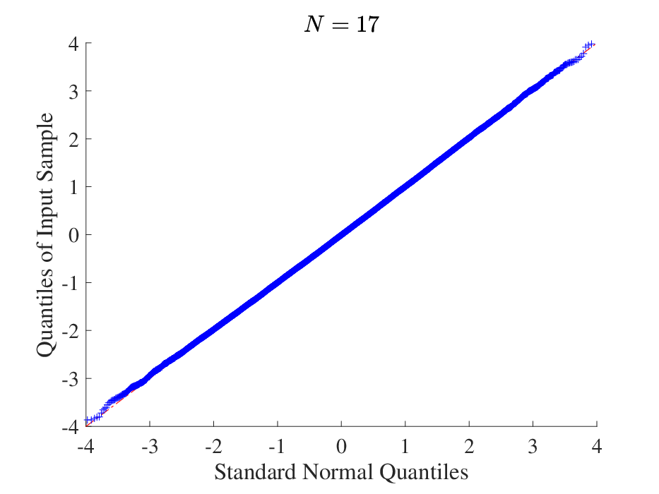
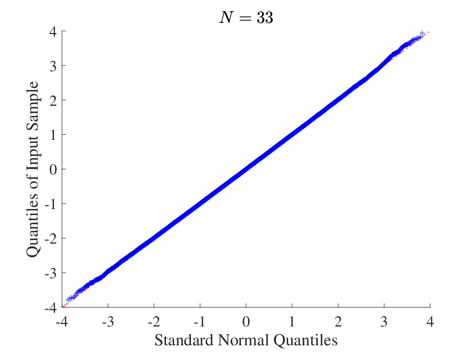
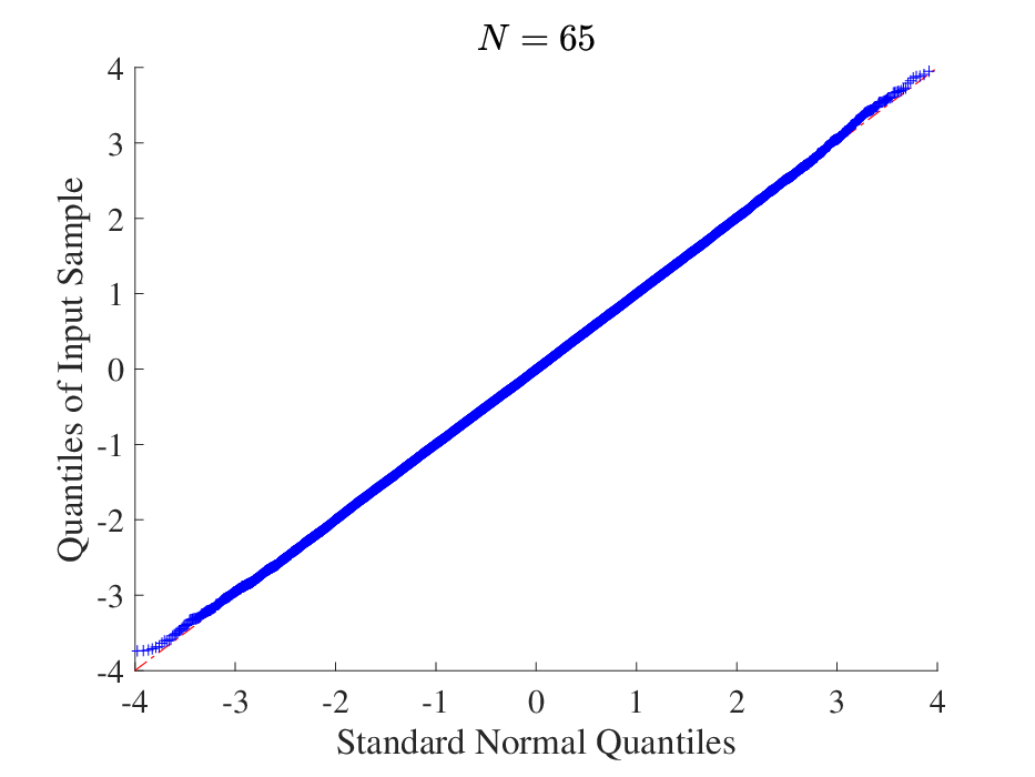
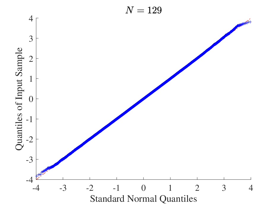
The rest of this paper is organized as follows. In Section II, the system model and problem formulation are introduced. In Section III, the main results regarding the first-order (EMI) and second-order (CLT) analysis with the convergence rates are presented, together with a moderate-to-high SNR approximation, which shows the impact of the number of effective scatterers. Section IV introduces the Gaussian tools and some preliminary results. The rigorous proof of the first-order and second-order analysis is given in Section V and Section VI, respectively. In Section VII, numerical experiments are performed to validate the Gaussianity of the MI and illustrate the approximation performance. Section VIII concludes the paper.

Notations: Matrices and vectors are denoted by the bold, upper case letters and bold, lower case letters, respectively. 𝔼​x\mathbb{E}x represents the expectation of xx and ℙ⁡(⋅)\mathbb{P}(\cdot) denotes the probability measure. (⋅)∗(\cdot)^{*} represents the conjugate of a complex number. ℂN\mathbb{C}^{N} and ℂM×N\mathbb{C}^{M\times N} denote the space of NN-dimensional vectors and the space of MM-by-NN matrices, respectively. 𝔸H\mathbb{A}^{H} represents the conjugate transpose of 𝔸\mathbb{A}, and the (i,j)(i,j)-th entry of 𝔸\mathbb{A} is denoted by Ai​jA_{ij}. ‖𝔸‖\|{\mathbb{A}}\| represents the spectral norm of 𝔸\mathbb{A}. Tr⁡𝔸\Tr{\mathbb{A}} refers to the trace of 𝔸{\mathbb{A}} if it is square. 𝕀N\mathbb{I}_{N} denotes the identity matrix of size NN. ϕ⁡(x)\phi(x) denotes the cumulative distribution function (CDF) of the standard Gaussian distribution. The complex partial derivative operators for a complex number z=x+ȷ​yz=x+\jmath y with ȷ=−1\jmath=\sqrt{-1} are given by ∂∂z=12​(∂∂x−ȷ​∂∂y)\frac{\partial}{\partial z}=\frac{1}{2}(\frac{\partial}{\partial x}-\jmath\frac{\partial}{\partial y}) and ∂∂z∗=12​(∂∂x+ȷ​∂∂y)\frac{\partial}{\partial{z}^{*}}=\frac{1}{2}(\frac{\partial}{\partial x}+\jmath\frac{\partial}{\partial y}), where ∂∂x\frac{\partial}{\partial x} and ∂∂y\frac{\partial}{\partial y} are standard partial derivatives with respect to xx and yy, respectively. δ⁡(⋅)\delta(\cdot) denotes the Kronecker function, i.e., δ⁡(0)=1\delta(0)=1 and δ⁡(m)=0,m≠0\delta(m)=0,~m\neq 0. x¯=x−𝔼​x\underline{x}=x-\mathbb{E}x denotes the centered form of a random variable xx and Cov⁡(x,y)=𝔼​x¯​y¯\mathrm{Cov}(x,y)=\mathbb{E}\underline{x}\underline{y} represents the covariance of xx and yy. 𝒪⁡(⋅){\mathcal{O}}(\cdot) and Θ⁡(⋅)\Theta(\cdot) denote the big-O and big-theta notations, respectively. Finally, →N→∞𝒟\xrightarrow[N\rightarrow\infty]{\mathcal{D}} denotes the convergence in distribution.

II System Model and Problem Formulation

II-A System Model

Consider a point-to-point MIMO system with MM transmit antennas and NN receive antennas. The received signal 𝕪∈ℂN\mathbb{y}\in\mathbb{C}^{N} can be given by

𝕪=ℍ​𝕤+𝕟,\mathbb{y}={\mathbb{H}}\mathbb{s}+\mathbb{n}, (1)

where 𝕤∈ℂM\mathbb{s}\in\mathbb{C}^{M} denotes the transmitted signal with covariance matrix 𝔼​𝕤​𝕤H=𝕎\mathbb{E}\mathbb{s}\mathbb{s}^{H}=\mathbb{W}, ℍ∈ℂN×M{\mathbb{H}}\in\mathbb{C}^{N\times M} represents the channel matrix, and 𝕟∈ℂN\mathbb{n}\in\mathbb{C}^{N} is the additive white Gaussian noise. The elements of 𝕟\mathbb{n} are i.i.d. and circularly Gaussian random variables with variance σ2\sigma^{2}. As a figure of merit for the performance over coherent MIMO fading channels, the MI is given by [31]

C(σ2)=logdet(𝕀N+1σ2ℍ𝕎ℍH).C(\sigma^{2})=\log\det(\mathbb{I}_{N}+\frac{1}{\sigma^{2}}{\mathbb{H}}{\mathbb{W}}{\mathbb{H}}^{H}). (2)

Given ℍ{\mathbb{H}} is a random matrix, C⁡(σ2)C(\sigma^{2}) is a random variable whose statistical properties deserve investigation. Specifically, the first-order and second-order analysis for C⁡(σ2)C(\sigma^{2}) can be used to evaluate the average throughput and outage probability. In this paper, we assume that only the statistical CSI is available at the transmitter.

II-B Channel Model

With statistical CSI, we consider the channel model given by

ℍ=ΦR12​𝕏​ΦS12​𝕐​ΦT12,{\mathbb{H}}=\mathbb{\Phi}_{R}^{\frac{1}{2}}{\mathbb{X}}\mathbb{\Phi}_{S}^{\frac{1}{2}}{\mathbb{Y}}\mathbb{\Phi}_{T}^{\frac{1}{2}}, (3)

where ΦR∈ℂN×N\mathbb{\Phi}_{R}\in\mathbb{C}^{N\times N}, ΦS∈ℂL×L\mathbb{\Phi}_{S}\in\mathbb{C}^{L\times L}, and ΦT∈ℂM×M\mathbb{\Phi}_{T}\in\mathbb{C}^{M\times M} represent the correlation matrices at the receiver, the scatterers, and the transmitter, respectively. 𝕏∈ℂN×L{\mathbb{X}}\in\mathbb{C}^{N\times L} and 𝕐∈ℂL×M{\mathbb{Y}}\in\mathbb{C}^{L\times M} are two random matrices, whose entries are i.i.d. and circularly Gaussian random variables with variances 1L\frac{1}{L} and 1M\frac{1}{M}, respectively. The model in (3) is a special Kronecker model with either a random receive correlation matrix or a random transmit correlation matrix. In practice, this model has the following applications.

1. Double-scattering channel: (3) was proposed in [1] to model the correlation at the transceiver and scatterers, and the rank of the channel. The rank-deficiency situation is reflected by the case with L<min⁡(M,N)L<\min(M,N). Without correlation at the transceivers and scatterers, the double-scattering model degenerates to the Rayleigh product model, also referred to as multi-keyhole channel[32], which is the product of two i.i.d. complex Gaussian matrices. Note that ΦS12\mathbb{\Phi}_{S}^{\frac{1}{2}} is a Hermitian matrix for a double-scattering channel.

2. Cascaded Channel in IRS-aided MIMO systems: (3) can also be used to model the cascaded channel in an IRS-aided MIMO system. Under such circumstances, we have ΦS12=𝕋12I​R​S​Ψ​ℝ12I​R​S\mathbb{\Phi}_{S}^{\frac{1}{2}}={\mathbb{T}^{\frac{1}{2}}}_{IRS}\mathbb{\Psi}{\mathbb{R}^{\frac{1}{2}}}_{IRS}, where 𝕋I​R​S{\mathbb{T}}_{IRS} and ℝI​R​S{\mathbb{R}}_{IRS} denote the transmit and receive correlation matrix of the IRS, respectively, and Ψ\mathbb{\Psi} represents the phase shifts matrix [15, 21]. In this case, ΦS12\mathbb{\Phi}_{S}^{\frac{1}{2}} may not be a Hermitian matrix.11 1 Note that this model and the related analysis for IRS-aided systems is only applicable when the statistical CSI is available. The statistical CSI based analysis and design has been widely used in IRS-aided systems [15, 21, 33, 34].

Given only the statistical CSI at the transmitter, we can assume the covariance matrix of the transmitted signal to be ℚ=𝕀M{\mathbb{Q}}=\mathbb{I}_{M}. This is because, for any given transmit covariance 𝕎{\mathbb{W}}, we can do the substitution ΦT′=ΦT12​𝕎​ΦTH2\mathbb{\Phi}_{T}^{\prime}=\mathbb{\Phi}_{T}^{\frac{1}{2}}{\mathbb{W}}\mathbb{\Phi}_{T}^{\frac{H}{2}} to construct a new correlation matrix ΦT′\mathbb{\Phi}_{T}^{\prime} at the transmitter such that the evaluation can be converted to the case with an identity transmit covariance matrix, i.e., C(σ2)=logdet(𝕀N+1σ2ℍ𝕎ℍH)=logdet(𝕀N+1σ2ℍ′ℍ′H)C(\sigma^{2})=\log\det(\mathbb{I}_{N}+\frac{1}{\sigma^{2}}{\mathbb{H}}{\mathbb{W}}{\mathbb{H}}^{H})=\log\det(\mathbb{I}_{N}+\frac{1}{\sigma^{2}}{\mathbb{H}}^{\prime}{\mathbb{H}}^{\prime H}), where ℍ′=ΦR12​𝕏​ΦS12​𝕐​ΦT′12{\mathbb{H}}^{\prime}=\mathbb{\Phi}_{R}^{\frac{1}{2}}{\mathbb{X}}\mathbb{\Phi}_{S}^{\frac{1}{2}}{\mathbb{Y}}\mathbb{\Phi}_{T}^{\prime\frac{1}{2}}.

II-C Problem Formulation

In the following, we will derive an equivalent channel model to simplify the evaluation of (2). Define the eigenvalue decompositions ΦR=𝕌R​ℝ​𝕌RH\mathbb{\Phi}_{R}=\mathbb{U}_{R}{\mathbb{R}}\mathbb{U}_{R}^{H}, ΦT=𝕌T​𝕋​𝕌TH\mathbb{\Phi}_{T}=\mathbb{U}_{T}\mathbb{T}\mathbb{U}_{T}^{H} and the singular value decomposition (SVD) ΦS12=𝕌S​𝕊12​𝕍SH\mathbb{\Phi}_{S}^{\frac{1}{2}}=\mathbb{U}_{S}{\mathbb{S}^{\frac{1}{2}}}\mathbb{V}_{S}^{H}, where ℝ\mathbb{R}, 𝕊\mathbb{S}, and 𝕋\mathbb{T} are diagonal matrices. Then, we can obtain

C⁡(σ2)\displaystyle C(\sigma^{2}) =logdet(𝕀N+1σ2ΦR12𝕏ΦS12𝕐ΦT𝕐HΦSH2𝕏HΦR12)\displaystyle=\log\det(\mathbb{I}_{N}+\frac{1}{\sigma^{2}}\mathbb{\Phi}_{R}^{\frac{1}{2}}{\mathbb{X}}\mathbb{\Phi}_{S}^{\frac{1}{2}}{\mathbb{Y}}\mathbb{\Phi}_{T}{\mathbb{Y}}^{H}\mathbb{\Phi}_{S}^{\frac{H}{2}}{\mathbb{X}}^{H}\mathbb{\Phi}_{R}^{\frac{1}{2}}) (4)
=logdet(𝕀N+1σ2𝕌Rℝ12𝕌RH𝕏𝕌S𝕊12𝕍SH𝕐𝕌T𝕋𝕌TH𝕐H𝕍S𝕊12𝕌SH𝕏H𝕌Rℝ12𝕌RH)\displaystyle=\log\det({\mathbb{I}}_{N}+\frac{1}{\sigma^{2}}\mathbb{U}_{R}\mathbb{R}^{\frac{1}{2}}\mathbb{U}_{R}^{H}\mathbb{X}\mathbb{U}_{S}\mathbb{S}^{\frac{1}{2}}\mathbb{V}_{S}^{H}\mathbb{Y}\mathbb{U}_{T}\mathbb{T}\mathbb{U}_{T}^{H}\mathbb{Y}^{H}\mathbb{V}_{S}\mathbb{S}^{\frac{1}{2}}\mathbb{U}_{S}^{H}\mathbb{X}^{H}\mathbb{U}_{R}\mathbb{R}^{\frac{1}{2}}\mathbb{U}_{R}^{H})
=(a)​log​det(𝕀N+1σ2​ℝ12​𝕏′​𝕊12​𝕐′​𝕋​𝕐′H​𝕊12​𝕏′H​ℝ12),\displaystyle\overset{(a)}{=}\log\det({\mathbb{I}}_{N}+\frac{1}{\sigma^{2}}\mathbb{R}^{\frac{1}{2}}\mathbb{X}^{\prime}\mathbb{S}^{\frac{1}{2}}\mathbb{Y}^{\prime}\mathbb{T}\mathbb{Y}^{\prime H}\mathbb{S}^{\frac{1}{2}}\mathbb{X}^{\prime H}\mathbb{R}^{\frac{1}{2}}),

where 𝕏′=𝕌RH​𝕏​𝕌S\mathbb{X}^{\prime}=\mathbb{U}_{R}^{H}\mathbb{X}\mathbb{U}_{S}, 𝕐′=𝕍SH​𝕐​𝕌T\mathbb{Y}^{\prime}=\mathbb{V}_{S}^{H}\mathbb{Y}\mathbb{U}_{T} and step (a)(a) follows from the identity det(𝕀+𝔸​𝔹)=det(𝕀+𝔹​𝔸)\det(\mathbb{I}+\mathbb{A}\mathbb{B})=\det(\mathbb{I}+\mathbb{B}\mathbb{A}). Given the unitary-invariant attribute of Gaussian random matrices, a Gaussian matrix 𝔾\mathbb{G} is equivalent to 𝔾′=𝕌​𝔾​𝕍\mathbb{G}^{\prime}=\mathbb{U}\mathbb{G}\mathbb{V} statistically, where 𝕌\mathbb{U} and 𝕍\mathbb{V} are both unitary matrices. Therefore, 𝕏\mathbb{X} (𝕐\mathbb{Y}) and 𝕏′\mathbb{X}^{\prime} (𝕐′\mathbb{Y}^{\prime}) are statistically equivalent. Thus, it is equivalent to consider the following channel

ℍ=ℝ12​𝕏​𝕊12​𝕐​𝕋12,{\mathbb{H}}=\mathbb{R}^{\frac{1}{2}}\mathbb{X}\mathbb{S}^{\frac{1}{2}}\mathbb{Y}\mathbb{T}^{\frac{1}{2}}, (5)

where ℝ=diag⁡(r1,r2,…,rN){\mathbb{R}}=\mathrm{diag}\left(r_{1},r_{2},...,r_{N}\right), 𝕊=diag⁡(s1,s2,…,sL){\mathbb{S}}=\mathrm{diag}\left(s_{1},s_{2},...,s_{L}\right), 𝕋=diag⁡(t1,t2,…,tM){\mathbb{T}}=\mathrm{diag}\left(t_{1},t_{2},...,t_{M}\right). In this paper, we will investigate the asymptotic distribution of the statistic C(σ2)=logdet(𝕀N+1σ2ℍℍH)C(\sigma^{2})=\log\det(\mathbb{I}_{N}+\frac{1}{\sigma^{2}}{\mathbb{H}}{\mathbb{H}}^{H}).

II-D Assumptions

The results of this paper are developed based on the following assumptions:

A.1. 0<liminfM≥1ML≤ML≤limsupM≥1ML<∞0<\lim\inf\limits_{M\geq 1}\frac{M}{L}\leq\frac{M}{L}\leq\lim\sup\limits_{M\geq 1}\frac{M}{L}<\infty and 0<liminfM≥1MN≤MN≤limsupM≥1MN<∞0<\lim\inf\limits_{M\geq 1}\frac{M}{N}\leq\frac{M}{N}\leq\lim\sup\limits_{M\geq 1}\frac{M}{N}<\infty,

A.2. limsupM≥1‖ℝ‖<∞\lim\sup\limits_{M\geq 1}\|{\mathbb{R}}\|<\infty, limsupM≥1‖𝕋‖<∞\lim\sup\limits_{M\geq 1}\|{\mathbb{T}}\|<\infty, and limsupM≥1‖𝕊‖<∞\lim\sup\limits_{M\geq 1}\|{\mathbb{S}}\|<\infty,

A.3. infM≥11M​Tr⁡ℝ>0\inf\limits_{M\geq 1}\frac{1}{M}\Tr{\mathbb{R}}>0, infM≥11M​Tr⁡𝕋>0\inf\limits_{M\geq 1}\frac{1}{M}\Tr{\mathbb{T}}>0, and infM≥11M​Tr⁡𝕊>0\inf\limits_{M\geq 1}\frac{1}{M}\Tr{\mathbb{S}}>0.

A.1 defines the asymptotic regime considered for the large-scale system, where the dimensions of the system (MM, NN, and LL) grow to infinity at the same pace. A.2 and A.3 restrict the rank of the correlation matrices so that the extremely low-rank case, i.e., the rank of the correlation matrix does not increase with the number of antennas, will not occur [7, 35].

The product of two random matrices makes it challenging to give an explicit expression for the distribution of the MI. In this paper, we will investigate the asymptotic distribution of the MI for double-scattering channels by setting up a CLT utilizing the Gaussian tools.

III Main Results

III-A Useful notations

Before presenting the main results, we first introduce some notations that will be utilized in this paper.

The Fundamental System of Equations) The asymptotic mean and variance in the CLT will be induced by the solution of the following system of equations with respect to (δ⁡(z),ω⁡(z),ω¯​(z))(\delta(z),\omega(z),\overline{\omega}(z)),

{δ⁡(z)=1L​Tr⁡ℝ​(z​𝕀N+M​ω​(z)​ω¯​(z)L​δ​(z)​ℝ)−1,ω⁡(z)=1M​Tr⁡𝕊​(1δ⁡(z)​𝕀L+ω¯​(z)​𝕊)−1,ω¯​(z)=1M​Tr⁡𝕋​(𝕀M+ω⁡(z)​𝕋)−1.\displaystyle\begin{cases}&\delta(z)=\frac{1}{L}\Tr\mathbb{R}\left(z\mathbb{I}_{N}+\frac{M\omega(z)\overline{\omega}(z)}{L\delta(z)}\mathbb{R}\right)^{-1},\\ &\omega(z)=\frac{1}{M}\Tr\mathbb{S}\left(\frac{1}{\delta(z)}\mathbb{I}_{L}+\overline{\omega}(z)\mathbb{S}\right)^{-1},\\ &\overline{\omega}(z)=\frac{1}{M}\Tr\mathbb{T}\left(\mathbb{I}_{M}+\omega(z)\mathbb{T}\right)^{-1}.\end{cases} (6)

For the simplicity of notations, we will omit zz in (δ⁡(z),ω⁡(z),ω¯​(z))(\delta(z),\omega(z),\overline{\omega}(z)) and use (δ,ω,ω¯)(\delta,\omega,\overline{\omega}) in the following derivation. The existence and uniqueness of the positive solution of (6) was proved in [14] by the standard interference function theory, which is widely utilized to show the existence and uniqueness of the solution for such fixed-point equations, e.g., [36, 37]. in the following derivation. The fixed-point algorithm for obtaining the solution was given in [38]. It was shown that the complexity of the algorithm is 𝒪⁡(log⁡(1ε)){\mathcal{O}}(\log(\frac{1}{\varepsilon})), where ε\varepsilon is the accuracy of the solution.

Resolvent) The resolvent matrix of ℍ​ℍH{\mathbb{H}}{\mathbb{H}}^{H} is given by

ℚ⁡(z)=(z​𝕀N+ℍ​ℍH)−1,{\mathbb{Q}}(z)=\left(z\mathbb{I}_{N}+{\mathbb{H}}{\mathbb{H}}^{H}\right)^{-1}, (7)

which will be shown to be highly related to the MI in Section V. The following resolvent identity holds true

z​ℚ​(z)=𝕀N−ℍ​ℍH​ℚ​(z).z{\mathbb{Q}}(z)=\mathbb{I}_{N}-{\mathbb{H}}{\mathbb{H}}^{H}{\mathbb{Q}}(z). (8)

For simplicity, we will denote ℚ⁡(z){\mathbb{Q}}(z) as ℚ{\mathbb{Q}} in the following.

Deterministic Approximations of the Resolvent Matrix) We define the following deterministic matrices

𝔾R\displaystyle{\mathbb{G}}_{R} =(z𝕀N+M​ω​ω¯L​δℝ)−1,𝔾S=(1δ𝕀L+ω¯𝕊)−1,𝔾T=(𝕀M+ω𝕋)−1,𝔽S=(𝕀L+δω¯𝕊)−1=1δ𝔾S.\displaystyle=\left(z\mathbb{I}_{N}+\frac{M\omega\overline{\omega}}{L\delta}\mathbb{R}\right)^{-1},{\mathbb{G}}_{S}=\left(\frac{1}{\delta}\mathbb{I}_{L}+\overline{\omega}\mathbb{S}\right)^{-1},{\mathbb{G}}_{T}=\left(\mathbb{I}_{M}+\omega\mathbb{T}\right)^{-1},~{\mathbb{F}}_{S}=\left(\mathbb{I}_{L}+\delta\overline{\omega}\mathbb{S}\right)^{-1}=\frac{1}{\delta}{\mathbb{G}}_{S}. (9)

𝔾R{\mathbb{G}}_{R} will be shown to be an approximation of 𝔼​ℚ​(z)\mathbb{E}{\mathbb{Q}}(z). Related notations induced by 𝔾R,𝔾S,𝔾T{\mathbb{G}}_{R},{\mathbb{G}}_{S},{\mathbb{G}}_{T} are presented in Table I, which will be used in the following derivation.

TABLE I: Table of Notations.
Notations Expression Notations Expression Notations Expression Notations Expression
νR\nu_{R} 1L​Tr⁡ℝ2​𝔾R2\frac{1}{L}\Tr\mathbb{R}^{2}{\mathbb{G}}_{R}^{2} νR,I\nu_{R,I} 1L​Tr⁡ℝ​𝔾R2\frac{1}{L}\Tr\mathbb{R}{\mathbb{G}}_{R}^{2} νS\nu_{S} 1M​Tr⁡𝕊2​𝔾S2\frac{1}{M}\Tr\mathbb{S}^{2}{\mathbb{G}}_{S}^{2} νS,I\nu_{S,I} 1M​Tr⁡𝕊​𝔾S2\frac{1}{M}\Tr\mathbb{S}{\mathbb{G}}_{S}^{2}
νT\nu_{T} 1M​Tr⁡𝕋2​𝔾T2\frac{1}{M}\Tr\mathbb{T}^{2}{\mathbb{G}}_{T}^{2} νT,I\nu_{T,I} 1M​Tr⁡𝕋​𝔾T2\frac{1}{M}\Tr\mathbb{T}{\mathbb{G}}_{T}^{2} ηR\eta_{R} 1L​Tr⁡ℝ3​𝔾R3\frac{1}{L}\Tr\mathbb{R}^{3}{\mathbb{G}}_{R}^{3} ηR,I\eta_{R,I} 1L​Tr⁡ℝ2​𝔾R3\frac{1}{L}\Tr\mathbb{R}^{2}{\mathbb{G}}_{R}^{3}
ηS\eta_{S} 1M​Tr⁡𝕊3​𝔾S3\frac{1}{M}\Tr\mathbb{S}^{3}{\mathbb{G}}_{S}^{3} ηS,I\eta_{S,I} 1M​Tr⁡𝕊2​𝔾S3\frac{1}{M}\Tr\mathbb{S}^{2}{\mathbb{G}}_{S}^{3} ηT\eta_{T} 1M​Tr⁡𝕋3​𝔾T3\frac{1}{M}\Tr\mathbb{T}^{3}{\mathbb{G}}_{T}^{3} ηT,I\eta_{T,I} 1M​Tr⁡𝕋2​𝔾T3\frac{1}{M}\Tr\mathbb{T}^{2}{\mathbb{G}}_{T}^{3}
ΔS\Delta_{S} 1−νS​νT1-\nu_{S}\nu_{T} Δ\Delta 1−M​ω​ω¯​νRL​δ2+M​νR​νS,I​νT,IL​δ3​ΔS1-\frac{M\omega\overline{\omega}\nu_{R}}{L\delta^{2}}+\frac{M\nu_{R}\nu_{S,I}\nu_{T,I}}{L\delta^{3}\Delta_{S}} θ\theta M​ω​ω¯L​δ2−M​νS,I​νT,IL​δ3​ΔS\frac{M\omega\overline{\omega}}{L\delta^{2}}-\frac{M\nu_{S,I}\nu_{T,I}}{L\delta^{3}\Delta_{S}}

III-B First-order Result

Theorem 1.

Given that assumptions A.1-A.3 hold true and (δ,ω,ω¯)(\delta,\omega,\overline{\omega}) is the positive solution of (6) when z=σ2z=\sigma^{2}, the EMI can be approximated by

𝔼​C​(σ2)=C¯​(σ2)+𝒪⁡(1N),\mathbb{E}C(\sigma^{2})=\overline{C}(\sigma^{2})+\mathcal{O}(\frac{1}{N}), (10)

where

C¯(σ2)=logdet(𝕀N+M​ω​ω¯σ2​L​δℝ)+logdet(𝕀L+δω¯𝕊)+logdet(𝕀M+ω𝕋)−2Mωω¯.\displaystyle\overline{C}(\sigma^{2})=\log\det(\mathbb{I}_{N}+\frac{M\omega\overline{\omega}}{\sigma^{2}L\delta}\mathbb{R})+\log\det(\mathbb{I}_{L}+\delta\overline{\omega}\mathbb{S})+\log\det(\mathbb{I}_{M}+\omega\mathbb{T})-2M\omega\overline{\omega}. (11)
Proof.

The proof of Theorem 1 will be given in Section V. ∎

Remark 1.

(Comparison with existing results) A similar approximation was first proposed in [12, Theorem 2] and [14, Theorem 5] but only the convergence of the normalized MI (MI per receive antenna) was guaranteed. The result about the normalized MI is also consistent with that shown in [15, Corollary 1] and [16, Proposition 1], which were derived by the replica method. The replica method is efficient in determining the deterministic approximation, but can not provide an exact convergence rate. In fact, the convergence rate of the EMI without normalization is not available in the literature. In this paper, by utilizing the Gaussian tools, we derive the approximation of the EMI and obtain a convergence rate. From Theorem 1, we can observe that the error of the deterministic approximation in (11) can be bounded by 𝒪⁡(1N){\mathcal{O}}(\frac{1}{N}). This convergence rate was also validated for single hop Gaussian channels [7], frequency selective channels [23], and Rician channels [22].

III-C Second-order Result

Theorem 2.

(CLT of the MI) Given the same setting as that in Theorem 1, the asymptotic distribution of the MI over double-scattering channel is Gaussian and the following convergence holds true

C⁡(σ2)−C¯​(σ2)V⁡(σ2)→N→∞𝒟𝒩⁡(0,1),\frac{C(\sigma^{2})-\overline{C}(\sigma^{2})}{\sqrt{V(\sigma^{2})}}\xrightarrow[N\rightarrow\infty]{\mathcal{D}}\mathcal{N}(0,1), (12)

where C¯​(σ2)\overline{C}(\sigma^{2}) is given in (11). The asymptotic variance V⁡(σ2)V(\sigma^{2}) can be expressed as

V⁡(σ2)\displaystyle V(\sigma^{2}) =−log⁡(Δ)−log⁡(ΔS),\displaystyle=-\log(\Delta)-\log(\Delta_{S}), (13)

where Δ\Delta and ΔS\Delta_{S} are given in Table I. Furthermore, the convergence of the variance is given by

Var⁡(C⁡(σ2))=V⁡(σ2)+𝒪⁡(1N),\mathrm{Var}(C(\sigma^{2}))=V(\sigma^{2})+{\mathcal{O}}(\frac{1}{N}), (14)

and the convergence rate of the characteristic function of C⁡(σ2)C(\sigma^{2}) is 𝒪⁡(1N){\mathcal{O}}(\frac{1}{N}).

Proof.

The proof of Theorem 2 will be given in Section VI. ∎

Remark 2.

(Non-Gaussian fading) The 𝒪⁡(1N){\mathcal{O}}(\frac{1}{N}) convergence rate of the asymptotic mean and variance is preserved by the Gaussianity of the two random matrices in (5), and will not hold for the product of non-Gaussian matrices. In [30], the linear spectral statistics (LSS) (mutual information is a special case of LSS by taking f⁡(x)=log⁡(1+xσ2)f(x)=\log(1+\frac{x}{\sigma^{2}})) of two i.i.d., real, non-Gaussian square matrices was investigated to show the asymptotic Gaussianity of the LSS but the asymptotic mean and variance are related to the fourth-order cumulant of entries of the two matrices, which is zero for Gaussian entries. This phenomenon has also been discovered in single-hop channels. The centered and non-centered non-Gaussian channels were investigated in [10], and [9, 35], respectively. These results indicate that compared with the mean and variance of Gaussian channels, the asymptotic mean and variance of non-Gaussian channels should be amended by terms related to the pseudo-variance and fourth-order cumulant of the complex entries, which are referred to as the bias. Therefore, it is reasonable to make a conjecture that the asymptotic Gaussianity of the MI still holds true for the two-hop non-Gaussian channels where the asymptotic mean and variance of the MI should be amended by adding a bias to the mean and variance derived in Theorem 2. The investigation of the bias for the product of two general non-Gaussian random matrices will be left as a future work.

Remark 3.

(Comparison with existing results)  [20] presented a CLT for the MI over Rayleigh product channel (i.i.d. double-scattering channel) by a free probability approach. The explicit expression for the variance was given for the case with N=MN=M, which is a special case of Theorem 2. Motivated by the thought of splitting the randomness into two parts with respect to two random matrices, [21, Theorem 2] derived the same result by using the resolvent method. However, how fast the distribution of C⁡(σ2)C(\sigma^{2}) converges to a Gaussian distribution and how fast the mean and the variance converge to their deterministic approximations are both unknown. In this paper, we recover the result in [21, Theorem 2] and show, for the first time, that the convergence rates of the variance and the characteristic function are 𝒪⁡(1N){\mathcal{O}}(\frac{1}{N}).

Proposition 1.

Given assumptions A.1, A.2, A.3, and a σ2>0\sigma^{2}>0, there exist two positive numbers bσ2b_{\sigma^{2}} and Bσ2B_{\sigma^{2}} satisfying

0<bσ2≤infNV⁡(σ2)≤supNV⁡(σ2)≤Bσ2≤∞.0<b_{\sigma^{2}}\leq\inf_{N}V(\sigma^{2})\leq\sup_{N}V(\sigma^{2})\leq B_{\sigma^{2}}\leq\infty. (15)
Proof.

The proof of Proposition 1 is given in Appendix E. ∎

Remark 4.

Proposition 1 indicates that the asymptotic variance V⁡(σ2)V(\sigma^{2}) is well-defined for a given σ2\sigma^{2}.

By Theorem 2, we can obtain a closed form approximation for the outage probability with a given rate RR as

po​u​t​(R)≈Φ⁡(R−C¯​(σ2)V⁡(σ2)).p_{out}(R)\approx\Phi(\frac{R-\overline{C}(\sigma^{2})}{\sqrt{V(\sigma^{2})}}). (16)

Conversely, given the outage probability po​u​tp_{out}, the outage rate, defined by

Cpo​u​t=sup{R≥0:ℙ⁡(C⁡(σ2)<R)≤po​u​t},C_{p_{out}}=\sup\{R\geq 0:\mathbb{P}(C({\sigma^{2}})<R)\leq p_{out}\}, (17)

can be approximated by Cpo​u​t≈C¯​(ρ)+V⁡(ρ)​Φ−1​(po​u​t)C_{p_{out}}\approx\overline{C}(\rho)+\sqrt{V(\rho)}\Phi^{-1}(p_{out}). Please note that (16) is obtained in a large system regime defined by A.1 and not applicable for the SNR-asymptotic regime [39]. However, the outage probability approximation in (16) can be utilized for the finite-SNR diversity-multiplexing trade-off (DMT) [40] analysis for two-hop channels, which was given in [21].

III-D i.i.d Case

To investigate the impact of the rank deficiency, we ignore the correlations and focus on the i.i.d. channel, i.e., Rayleigh product channel. In this case, the results will only be related to the ratios between the numbers of antennas and scatterers, denoted by η=NM\eta=\frac{N}{M} and κ=ML\kappa=\frac{M}{L}.

Proposition 2.

(Rayleigh-product channel) Given Assumption A.1, the asymptotic distribution of the MI over i.i.d. double-scattering channel is Gaussian and the following convergence holds true

Ci​i​d​(σ2)−C¯i​i​d​(σ2)Vi​i​d​(σ2)→N→∞𝒟𝒩⁡(0,1),\frac{C_{iid}(\sigma^{2})-\overline{C}_{iid}(\sigma^{2})}{\sqrt{V_{iid}(\sigma^{2})}}\xrightarrow[N\xrightarrow{}\infty]{\mathcal{D}}\mathcal{N}(0,1), (18)

where C¯i​i​d\overline{C}_{iid} and Vi​i​dV_{iid} are given by

C¯i​i​d​(σ2)\displaystyle\overline{C}_{iid}(\sigma^{2}) =M⁡[log⁡(1+ω)−(η−1κ)​log⁡(1−ωη⁡(1+ω))−log⁡(σ2)κ−log⁡(ω)κ−2​ω1+ω],\displaystyle=M[\log(1+\omega)-(\eta-\frac{1}{\kappa})\log(1-\frac{\omega}{\eta(1+\omega)})-\frac{\log(\sigma^{2})}{\kappa}-\frac{\log(\omega)}{\kappa}-\frac{2\omega}{1+\omega}], (19)
Vi​i​d​(σ2)\displaystyle V_{iid}(\sigma^{2}) =−log⁡(Δi​i​d),\displaystyle=-\log(\Delta_{iid}),

with

Δi​i​d=(1+δ​ω¯2)​δ​(σ2+κ​ω​ω¯2δ⁡(1+δ​ω¯2))η​κ​(1+δ​ω¯).\Delta_{iid}=\frac{(1+\delta\overline{\omega}^{2})\delta(\sigma^{2}+\frac{\kappa\omega\overline{\omega}^{2}}{\delta(1+\delta\overline{\omega}^{2})})}{\eta\kappa(1+\delta\overline{\omega})}. (20)

Here ω\omega is the root of the following cubic equation

P⁡(σ2)=ω3+(2​σ2+η​κ−κ−η+1)​ω2σ2+(1+η​κσ2−2​ησ2+1σ2)​ω−ησ2=0,\displaystyle P(\sigma^{2})=\omega^{3}+(2\sigma^{2}+\eta\kappa-\kappa-\eta+1)\frac{\omega^{2}}{\sigma^{2}}+(1+\frac{\eta\kappa}{\sigma^{2}}-\frac{2\eta}{\sigma^{2}}+\frac{1}{\sigma^{2}})\omega-\frac{\eta}{\sigma^{2}}=0, (21)

which satisfies ω>0\omega>0 and η+(η−1)​ω>0\eta+(\eta-1)\omega>0, and

δ\displaystyle\delta =1σ2​(NL−M​ωL⁡(1+ω)),ω¯\displaystyle=\frac{1}{\sigma^{2}}(\frac{N}{L}-\frac{M\omega}{L(1+\omega)}),~~~\overline{\omega} =11+ω.\displaystyle=\frac{1}{1+\omega}. (22)
Proof.

Proposition 2 can be obtained by letting ℝ=𝕀N{\mathbb{R}}={\mathbb{I}}_{N}, 𝕊=𝕀L{\mathbb{S}}={\mathbb{I}}_{L}, and 𝕋=𝕀M{\mathbb{T}}={\mathbb{I}}_{M} in Theorem 2 and the proof is omitted here. ∎

Remark 5.

(From Rayleigh-product channel to single-Rayleigh channel) In the following, we will show that when κ→0\kappa\xrightarrow{}0 and η=𝒪⁡(1)\eta={\mathcal{O}}(1), i.e., the number of scatterers is far larger than the number of antennas, the results in Proposition 2 degenerate to those for the of i.i.d. Rayleigh channel. When κ→0\kappa\xrightarrow{}0, equation (21) becomes

ω2+(1−ησ2+1σ2)​ω−ησ2=0,\omega^{2}+(1-\frac{\eta}{\sigma^{2}}+\frac{1}{\sigma^{2}})\omega-\frac{\eta}{\sigma^{2}}=0, (23)

whose positive solution is given by

ω0=ρ⁡(η−1)−1+[ρ⁡(η−1)−1]2+4​η​ρ2=ρ⁡(η−1)−1+ρ2​(η+1)2+2​ρ​(η+1)+1−4​ρ2​η2.\omega_{0}=\frac{\rho(\eta-1)-1+\sqrt{[\rho(\eta-1)-1]^{2}+4\eta\rho}}{2}=\frac{\rho(\eta-1)-1+\sqrt{\rho^{2}(\eta+1)^{2}+2\rho(\eta+1)+1-4\rho^{2}\eta}}{2}. (24)

Denote

v⁡(η,ρ)=ω01+ω0=η+1+σ2−(1+σ2+η)2−4​η2,v(\eta,\rho)=\frac{\omega_{0}}{1+\omega_{0}}=\frac{\eta+1+\sigma^{2}-\sqrt{(1+\sigma^{2}+\eta)^{2}-4\eta}}{2}, (25)

which is identical to [41, Eq. (11)]. We can also obtain from (22) that

L​δ0M=1σ2​(η−ω01+ω0)​=(a)​ω0,\frac{L\delta_{0}}{M}=\frac{1}{\sigma^{2}}(\eta-\frac{\omega_{0}}{1+\omega_{0}})\overset{(a)}{=}\omega_{0}, (26)

where (a)(a) follows from (23). We can rewrite C¯i​i​d​(σ2)\overline{C}_{iid}(\sigma^{2}) as

C¯i​i​d​(σ2)=M⁡[η​log⁡(1+κ​ω​ω¯σ2​δ)+1κ​log⁡(1+δ​ω¯)+log⁡(1+ω)−2​ω​ω¯]→κ→0\displaystyle\overline{C}_{iid}(\sigma^{2})=M[\eta\log(1+\frac{\kappa\omega\overline{\omega}}{\sigma^{2}\delta})+\frac{1}{\kappa}\log(1+\delta\overline{\omega})+\log(1+\omega)-2\omega\overline{\omega}]\xrightarrow{\kappa\rightarrow 0} (27)
M⁡[η​log⁡(1+1σ2​(1+ω0))+log⁡(1+ω0)−ω01+ω0]=M⁡[η​log⁡(1+ρ−ρ​v​(η,ρ))+log⁡(1+η​ρ−ρ​v​(η,ρ))−v⁡(η,ρ)],\displaystyle M[\eta\log(1+\frac{1}{\sigma^{2}(1+\omega_{0})})+\log(1+\omega_{0})-\frac{\omega_{0}}{1+\omega_{0}}]=M[\eta\log(1+\rho-\rho v(\eta,\rho))+\log(1+\eta\rho-\rho v(\eta,\rho))-v(\eta,\rho)],

which coincides with [41, Eq. (11)]. Now we turn to evaluate the variance. By (20), we have

Δi​i​d→κ→0ω0​(σ2+1(1+ω0)2)η=ω0​σ2+ω01+ω0−ω02(1+ω0)2η=1−ω02η​(1+ω0)2=1−v​(η,ρ)2η,\Delta_{iid}\xrightarrow{\kappa\rightarrow 0}\frac{\omega_{0}(\sigma^{2}+\frac{1}{(1+\omega_{0})^{2}})}{\eta}=\frac{\omega_{0}\sigma^{2}+\frac{\omega_{0}}{1+\omega_{0}}-\frac{\omega_{0}^{2}}{(1+\omega_{0})^{2}}}{\eta}=1-\frac{\omega_{0}^{2}}{\eta(1+\omega_{0})^{2}}=1-\frac{v(\eta,\rho)^{2}}{\eta}, (28)

and Vi​i​d​(σ2)→κ→0−log⁡(1−v​(η,ρ)2η)V_{iid}(\sigma^{2})\xrightarrow{\kappa\rightarrow 0}-\log\left(1-\frac{v(\eta,\rho)^{2}}{\eta}\right), which is the same as [41, Eq. (13)]. Therefore, when κ→0\kappa\xrightarrow{}0, the results for the Rayleigh-product channel degenerate to those for the i.i.d. single Rayleigh channel.

Remark 6.

(Extreme rank-deficient case) Different from Remark 5, here we consider the case when LL is finite but MM and NN go to infinity with the same pace, i.e., κ→∞\kappa\xrightarrow{}\infty. Under such circumstances, by analyzing the coefficient of the dominating term κ\kappa at the LHS of (21), we can obtain ω→κ→∞0\omega\xrightarrow{\kappa\xrightarrow{}\infty}0 and

ρ​κ​η​ω−η​ρ→κ→∞0,\displaystyle\rho\kappa\eta\omega-\eta\rho\xrightarrow{\kappa\xrightarrow{}\infty}0, (29)

so that we can obtain the solution of (21) as ω∞=κ−1+(1−η​ρ)​κ−2η​ρ+𝒪⁡(κ−3)\omega_{\infty}=\kappa^{-1}+\frac{(1-\eta\rho)\kappa^{-2}}{\eta\rho}+{\mathcal{O}}(\kappa^{-3}) and δ∞=η​κσ2−1σ2+𝒪⁡(κ−1)\delta_{\infty}=\frac{\eta\kappa}{\sigma^{2}}-\frac{1}{\sigma^{2}}+{\mathcal{O}}(\kappa^{-1}). In this case, we have

C¯i​i​d​(σ2)\displaystyle\overline{C}_{iid}(\sigma^{2}) =M⁡[log⁡(1+ω)−(η−1κ)​log⁡(1−ωη⁡(1+ω))−log⁡(σ2)κ−log⁡(ω)κ+log⁡(η)κ−2​ω1+ω]\displaystyle=M[\log(1+\omega)-(\eta-\frac{1}{\kappa})\log(1-\frac{\omega}{\eta(1+\omega)})-\frac{\log(\sigma^{2})}{\kappa}-\frac{\log(\omega)}{\kappa}+\frac{\log(\eta)}{\kappa}-\frac{2\omega}{1+\omega}] (30)
≈2​L−L​log⁡(σ2)+L​log⁡(ML)+L​log⁡(η)−2​L=L​log⁡(NL​σ2).\displaystyle\approx 2L-L\log(\sigma^{2})+L\log(\frac{M}{L})+L\log(\eta)-2L=L\log(\frac{N}{L\sigma^{2}}).

This indicates that, if LL is fixed, increasing MM and NN will result in an 𝒪⁡(log⁡(N)){\mathcal{O}}(\log(N)) increase in the ergodic rate. However, we can obtain from (30) that increasing LL, MM, and NN with the same pace will result in an NN increase in the ergodic rate. By plugging ω∞\omega_{\infty} and δ∞\delta_{\infty} into (20), we can evaluate the variance as

Vi​i​d​(σ2)\displaystyle V_{iid}(\sigma^{2}) =−log⁡(Δi​i​d)=−log⁡(1−1+ηη​κ)+𝒪⁡(κ−2)=𝒪⁡(κ−1),\displaystyle=-\log(\Delta_{iid})=-\log(1-\frac{1+\eta}{\eta\kappa})+{\mathcal{O}}(\kappa^{-2})={\mathcal{O}}(\kappa^{-1}), (31)

where

Δi​i​d\displaystyle\Delta_{iid} =(1+δ​ω¯2)​δ​(σ2+κ​ω​ω¯2δ⁡(1+δ​ω¯2))η​κ​(1+δ​ω¯)=(1−κ−1+𝒪⁡(κ−2))​(σ2+𝒪⁡(κ−2))​1−η−1​κ−1+𝒪⁡(κ−2)σ2\displaystyle=\frac{(1+\delta\overline{\omega}^{2})\delta(\sigma^{2}+\frac{\kappa\omega\overline{\omega}^{2}}{\delta(1+\delta\overline{\omega}^{2})})}{\eta\kappa(1+\delta\overline{\omega})}=(1-\kappa^{-1}+{\mathcal{O}}(\kappa^{-2}))(\sigma^{2}+{\mathcal{O}}(\kappa^{-2}))\frac{1-\eta^{-1}\kappa^{-1}+{\mathcal{O}}(\kappa^{-2})}{\sigma^{2}} (32)
=1−1+ηη​κ+𝒪⁡(κ−2).\displaystyle=1-\frac{1+\eta}{\eta\kappa}+{\mathcal{O}}(\kappa^{-2}).

The variance is of order 𝒪⁡(κ−1)=𝒪⁡(1M){\mathcal{O}}(\kappa^{-1})={\mathcal{O}}(\frac{1}{M}), which vanishes as MM goes to infinity. By Markov’s inequality, we can obtain that for any given positive ε\varepsilon, there holds true that

ℙ⁡(|Ci​i​d​(σ2)−𝔼​Ci​i​d​(σ2)|>ε)=ℙ⁡(|Ci​i​d​(σ2)−𝔼​Ci​i​d​(σ2)|2>ε2)≤Var⁡(Ci​i​d​(σ2))ε2→κ→∞0,\mathbb{P}(|C_{iid}(\sigma^{2})-\mathbb{E}C_{iid}(\sigma^{2})|>\varepsilon)=\mathbb{P}(|C_{iid}(\sigma^{2})-\mathbb{E}C_{iid}(\sigma^{2})|^{2}>\varepsilon^{2})\leq\frac{\mathrm{Var}(C_{iid}(\sigma^{2}))}{\varepsilon^{2}}\xrightarrow{\kappa\xrightarrow{}\infty}0, (33)

which indicates that Ci​i​d​(σ2)C_{iid}(\sigma^{2}) converges to its expectation in probability. Therefore, if LL is fixed and MM, NN go to infinity with the same pace, Ci​i​d​(σ2)C_{iid}(\sigma^{2}) tends to be deterministic.

III-E Moderate-to-High SNR Approximation

To investigate the impact of the system dimensions on the mean and variance of the MI, we give the moderate-to-high SNR approximation of the mean and variance for the Rayleigh-product channel by the following proposition.

Proposition 3.

(The impact of the number of scatterers) Denote (SN,SL,SM)(S_{N},S_{L},S_{M}) as the rearranged version of (N,L,M)(N,L,M) in the descending order, i.e., SN≥SL≥SMS_{N}\geq S_{L}\geq S_{M} and {SN,SL,SM}={N,L,M}\{S_{N},S_{L},S_{M}\}=\{N,L,M\}. Given ρ=1σ2\rho=\frac{1}{\sigma^{2}}, the mean C¯i​i​d​(ρ−1)\overline{C}_{iid}(\rho^{-1}) and variance Vi​i​d​(ρ−1){V}_{iid}(\rho^{-1}) of the MI can be approximated by

C¯i​i​d​(ρ−1)=\displaystyle\overline{C}_{iid}(\rho^{-1})\!\!= SM​log⁡(ρ​Ne2​SM)−(SN−SM)​log⁡(1−SMSN)−(SL−SM)​log⁡(1−SMSL)+𝒪⁡(ρ−1),when​SL≠SM,\displaystyle S_{M}\log(\frac{\rho N}{e^{2}S_{M}})\!-\!(S_{N}-S_{M})\log(1-\frac{S_{M}}{S_{N}})\!-\!(S_{L}-S_{M})\log(1-\frac{S_{M}}{S_{L}})+{\mathcal{O}}(\rho^{-1}),~\text{when}~S_{L}\neq S_{M}, (34a)
C¯i​i​d​(ρ−1)=\displaystyle\overline{C}_{iid}(\rho^{-1})\!\!= SM​log⁡(ρ​Ne2​SM)−(SN−SM)​log⁡(1−SMSN)+2​SM​(N​ρSM)−12(1−SMSN)12+𝒪⁡(ρ−1),when​SL=SM≠SN,\displaystyle S_{M}\log(\frac{\rho N}{e^{2}S_{M}})\!-\!(S_{N}-S_{M})\log(1-\frac{S_{M}}{S_{N}})+\frac{2S_{M}(\frac{N\rho}{S_{M}})^{-\frac{1}{2}}}{(1-\frac{S_{M}}{S_{N}})^{\frac{1}{2}}}+{\mathcal{O}}(\rho^{-1}),~\text{when}~S_{L}=S_{M}\neq S_{N}, (34b)
C¯i​i​d​(ρ−1)=\displaystyle\overline{C}_{iid}(\rho^{-1})\!\!= SM​log⁡(ρe2)+3​SM​ρ−13+𝒪⁡(ρ−23),when​SL=SM=SN.\displaystyle S_{M}\log(\frac{\rho}{e^{2}})+3S_{M}\rho^{-\frac{1}{3}}+{\mathcal{O}}(\rho^{-\frac{2}{3}}),~\text{when}~S_{L}=S_{M}=S_{N}. (34c)
Vi​i​d​(ρ−1)=\displaystyle V_{iid}(\rho^{-1})= −log⁡((1−SMSL)​(1−SMSN))+𝒪⁡(ρ−1),when​SL≠SM,\displaystyle-\log((1-\frac{S_{M}}{S_{L}})(1-\frac{S_{M}}{S_{N}}))+{\mathcal{O}}(\rho^{-1}),~\text{when}~S_{L}\neq S_{M}, (35a)
Vi​i​d​(ρ−1)=\displaystyle V_{iid}(\rho^{-1})= 12​log⁡(ρ​N4​(1−SMSN)​SM)+(1−2​SMSN)​(N​ρSM)−12(1−SMSN)12+𝒪⁡(ρ−1),when​SL=SM≠SN,\displaystyle\frac{1}{2}\log(\frac{\rho N}{4(1-\frac{S_{M}}{S_{N}})S_{M}})+\frac{(1-\frac{2S_{M}}{S_{N}})(\frac{N\rho}{S_{M}})^{-\frac{1}{2}}}{(1-\frac{S_{M}}{S_{N}})^{\frac{1}{2}}}+{\mathcal{O}}(\rho^{-1}),~\text{when}~S_{L}=S_{M}\neq S_{N}, (35b)
Vi​i​d​(ρ−1)=\displaystyle V_{iid}(\rho^{-1})= 2​log⁡(ρ)3−log⁡(3)+4​ρ−133+𝒪⁡(ρ−23),when​SL=SM=SN.\displaystyle\frac{2\log(\rho)}{3}-\log(3)+\frac{4\rho^{-\frac{1}{3}}}{3}+{\mathcal{O}}(\rho^{-\frac{2}{3}}),~\text{when}~S_{L}=S_{M}=S_{N}. (35c)
Proof.

The proof of Proposition 3 is given in Appendix I. ∎

Remark 7.

From (34c) and (35c), we can obtain that the approximations of C¯i​i​d​(ρ−1)\overline{C}_{iid}(\rho^{-1}) and Vi​i​d​(ρ−1){V}_{iid}(\rho^{-1}) are only determined by NN and the ordered (N,L,M)(N,L,M). A similar phenomenon was also noticed when investigating the DMT in [42]. We can observe that C¯i​i​d​(ρ−1)\overline{C}_{iid}(\rho^{-1}) grows in 𝒪⁡(log⁡(ρ)){\mathcal{O}}(\log(\rho)) when ρ\rho increases and the increasing speed, i.e., the coefficient of log⁡(ρ)\log(\rho), is determined by SMS_{M}, which is the minimum of (N,L,M)(N,L,M). The impact of the number of the scatterers can be observed from the dominating term in the mean and variance. When SM=LS_{M}=L, the multiplexing gain is limited by L, and increasing N and M will not help. Meanwhile, when L>max⁡{M,N}L>\max\{M,N\}, large LL does not contribute to the multiplexing gain although it helps for the diversity gain, which agrees with the result in [5, Example 6] and that for the IRS-aided MIMO channel in [21, Theorem 5].

Remark 8.

(Comparison between Rayleigh-product and single Rayleigh channel) The moderate-to-high SNR approximation for the mean and variance of the i.i.d. Rayleigh channels is given by [40, Eq.(13),(14)],

C¯R​a​y​l​e​i​g​h​(ρ−1)≈UM​log⁡(ρ​Ne​UM)−(UN−UM)​log⁡(1−UMUN),\overline{C}_{Rayleigh}(\rho^{-1})\approx U_{M}\log(\frac{\rho N}{eU_{M}})-(U_{N}-U_{M})\log(1-\frac{U_{M}}{U_{N}}), (36)
VR​a​y​l​e​i​g​h​(ρ−1)≈\displaystyle V_{Rayleigh}(\rho^{-1})\approx −log⁡(1−UMUN),UM≠UN,\displaystyle-\log(1-\frac{U_{M}}{U_{N}}),~~~U_{M}\neq U_{N}, (37a)
VR​a​y​l​e​i​g​h​(ρ−1)≈\displaystyle V_{Rayleigh}(\rho^{-1})\approx 12​[log⁡(ρ4)+2​ρ−12],UM=UN,\displaystyle\frac{1}{2}[\log(\frac{\rho}{4})+2\rho^{-\frac{1}{2}}],~~~U_{M}=U_{N}, (37b)

where UM=min⁡{M,N}U_{M}=\min\{M,N\} and UN=max⁡{M,N}U_{N}=\max\{M,N\}. From (36), we can observe that the multiplexing gain of the single Rayleigh channel is also limited by the minimum dimension. For the Rayleigh-product channel, when L<UML<U_{M}, i.e., LL is the smallest among N,LN,L, and MM, the loss of the ergodic rate due to rank deficiency is reflected by the coefficient LL of the dominating term in (34c). When L>UML>U_{M}, by comparing (34a) and (36), the loss of the ergodic rate is reflected by the 𝒪⁡(1){\mathcal{O}}(1) term, which is SM​(−1−(LSM−1)​log⁡(1−SML))<0S_{M}(-1-(\frac{L}{S_{M}}-1)\log(1-\frac{S_{M}}{L}))<0 (f⁡(x)=(1x−1)​log⁡(1−x)f(x)=(\frac{1}{x}-1)\log(1-x) is an increasing function so that f⁡(x)>−1f(x)>-1 when 0<x<10<x<1). When L→∞L\rightarrow\infty, the loss vanishes and (34a) becomes (36). From the high-order terms, i.e., 𝒪⁡(ρ−12){\mathcal{O}}(\rho^{-\frac{1}{2}}) in (34b) and 𝒪⁡(ρ−13){\mathcal{O}}(\rho^{-\frac{1}{3}}) in (34c), we can observe that the condition SL=SMS_{L}=S_{M} will affect the high order behavior, which also happens for the single Rayleigh case. In fact, according to (25) and (27), (36) can be further written as

C¯R​a​y​l​e​i​g​h​(ρ−1)={UM​log⁡(ρ​Ne​UM)−(UN−UM)​log⁡(1−UMUN)+𝒪⁡(ρ−1),UM≠UNUM​log⁡(ρe)+2​UM​ρ−12+𝒪⁡(ρ−1),UM=UN,\overline{C}_{Rayleigh}(\rho^{-1})=\begin{cases}U_{M}\log(\frac{\rho N}{eU_{M}})-(U_{N}-U_{M})\log(1-\frac{U_{M}}{U_{N}})+{\mathcal{O}}(\rho^{-1}),~~~U_{M}\neq U_{N}\\ U_{M}\log(\frac{\rho}{e})+2U_{M}\rho^{-\frac{1}{2}}+{\mathcal{O}}(\rho^{-1}),~~~U_{M}=U_{N},\end{cases} (38)

where the case with UM=UNU_{M}=U_{N} coincides with (34b) when L→∞L\rightarrow\infty.

For the variance, (37a) and (37b) can be obtained by letting κ→0\kappa\rightarrow 0 in (35a) and (35b), respectively. When L<UML<U_{M}, the impact of the rank deficiency is reflected by the dominating term, −log⁡((1−LM)​((1−LN)))-\log((1-\frac{L}{M})((1-\frac{L}{N}))). When L<L0=12​{UM+UN−[(UN−UM)​(3​UM+UN)]12}L<L_{0}=\frac{1}{2}\{U_{M}+U_{N}-[(U_{N}-U_{M})(3U_{M}+U_{N})]^{\frac{1}{2}}\}, −log⁡((1−LM)​((1−LN)))<−log⁡(1−UMUN)-\log((1-\frac{L}{M})((1-\frac{L}{N})))<-\log(1-\frac{U_{M}}{U_{N}}). When L0<L<UML_{0}<L<U_{M}, −log⁡((1−LM)​((1−LN)))>−log⁡(1−UMUN)-\log((1-\frac{L}{M})((1-\frac{L}{N})))>-\log(1-\frac{U_{M}}{U_{N}}). When L>UM≠UNL>U_{M}\neq U_{N}, the Rayleigh-product channel has a larger variance and the increment is −log⁡(1−UML)-\log(1-\frac{U_{M}}{L}). When M=NM=N and L>ML>M, the dominating terms in (35b) and (37b) are same and the increment of the variance is −12​log⁡[4​(1−ML)]-\frac{1}{2}\log[4(1-\frac{M}{L})]. From (35c), we can observe that the maximum variance occurs when M=N=LM=N=L.

Remark 9.

Proposition 3 provides an approximation for the asymptotic mean and variance given by Proposition 2 when the SNR ρ\rho is high. One may observe from the proof of Theorem 1 and the bound of the error in (186) that the approximation error for the asymptotic mean is 𝒪⁡(𝒫8​(1z)M​z){\mathcal{O}}(\frac{\mathcal{P}_{8}(\frac{1}{z})}{Mz}), which is guaranteed to be o⁡(1)o(1) when 1z\frac{1}{z} is 𝒪⁡(M1−ε9){\mathcal{O}}(M^{\frac{1-\varepsilon}{9}}), where 0<ε<10<\varepsilon<1. This means that 𝔼​Ci​i​d​(σ2)\mathbb{E}C_{iid}(\sigma^{2}) converges to the high SNR approximations in (34c) when MM, NN, LL go to infinity with the same pace and ρ\rho grows to infinity with the order 𝒪⁡(M1−ε9){\mathcal{O}}(M^{\frac{1-\varepsilon}{9}}). The approximation works well in the moderate-to-high SNR region, which is validated by simulations in Section VII. Note that there should be bounds better than 𝒪⁡(M1−ε9){\mathcal{O}}(M^{\frac{1-\varepsilon}{9}}) and a larger ρ\rho may also be shown to be tight.

IV Methodology and Preliminary Results

In this section, we will first present the main technique used in this paper, i.e., the Gaussian tools. Then, we will introduce some preliminary results obtained by this approach that will be useful for the following derivation.

IV-A Gaussian Tools

The Gaussian tools consist of two parts, i.e., Nash-Poincaré Inequality and the Integration by Parts Formula.

1. Nash-Poincaré Inequality Denote 𝕩=[x1,…,xN]T\mathbb{x}=[x_{1},...,x_{N}]^{T} as a complex Gaussian random vector satisfying 𝔼​𝕩=𝟘\mathbb{E}\mathbb{x}=\mathbb{0}, 𝔼​𝕩​𝕩T=𝟘\mathbb{E}\mathbb{x}\mathbb{x}^{T}=\mathbb{0}, and 𝔼​𝕩​𝕩H=Ω\mathbb{E}\mathbb{x}\mathbb{x}^{H}=\mathbb{\Omega}. f=f⁡(𝕩,𝕩∗)f=f(\mathbb{x},\mathbb{x}^{*}) is a ℂ1\mathbb{C}^{1} complex function such that both itself and its derivatives are polynomially bounded. Then, the variance of ff satisfies the following inequality, [7, Eq. (18)], [43, Proposition 2.5],

Var⁡[f⁡(𝕩,𝕩∗)]≤𝔼⁡[∇𝕩f​(𝕩,𝕩∗)T​Ω​∇𝕩f​(𝕩,𝕩∗)∗]+𝔼⁡[∇𝕩∗f​(𝕩,𝕩∗)H​Ω​∇𝕩∗f​(𝕩,𝕩∗)],\mathrm{Var}[f(\mathbb{x},\mathbb{x}^{*})]\leq\mathbb{E}[\nabla_{\mathbb{x}}f(\mathbb{x},\mathbb{x}^{*})^{T}\mathbb{\Omega}\nabla_{\mathbb{x}}f(\mathbb{x},\mathbb{x}^{*})^{*}]+\mathbb{E}[\nabla_{\mathbb{x}^{*}}f(\mathbb{x},\mathbb{x}^{*})^{H}\mathbb{\Omega}\nabla_{\mathbb{x}^{*}}f(\mathbb{x},\mathbb{x}^{*})], (39)

where ∇𝕩f​(𝕩)=[∂f∂x1,…,∂f∂xN]T\nabla_{\mathbb{x}}f(\mathbb{x})=[\frac{\partial f}{\partial x_{1}},...,\frac{\partial f}{\partial x_{N}}]^{T} and ∇𝕩∗f​(𝕩)=[∂f∂x1∗,…,∂f∂xN∗]T\nabla_{\mathbb{x}^{*}}f(\mathbb{x})=[\frac{\partial f}{\partial x_{1}^{*}},...,\frac{\partial f}{\partial x_{N}^{*}}]^{T}. (39) is referred to as the Nash-Poincaré inequality, which gives an upper bound for functional Gaussian random variables and is widely involved in the error estimation for the expectation of Gaussian matrices. By utilizing this inequality, the authors of [7, 22] showed that the approximation error of the deterministic approximation for the MI of single-hop MIMO channels is 𝒪⁡(1N){\mathcal{O}}(\frac{1}{N}). In this work, we will use this inequality to bound the error between the expectations and their deterministic approximations to obtain the convergence rate of the EMI and characteristic function of the MI for double-scattering channels.

2. Integration by Parts Formula [7, Eq. (17)]

𝔼⁡[xi​f​(𝕩,𝕩∗)]=∑m=1N[Ω]i,m​𝔼​[∂f⁡(𝕩,𝕩∗)∂xm∗].\mathbb{E}[x_{i}f(\mathbb{x},\mathbb{x}^{*})]=\sum_{m=1}^{N}[\mathbb{\Omega}]_{i,m}\mathbb{E}[\frac{\partial f(\mathbb{x},\mathbb{x}^{*})}{\partial x_{m}^{*}}]. (40)

If Ω=𝕀N\mathbb{\Omega}=\mathbb{I}_{N}, (40) can be simplified as

𝔼⁡[xi​f​(𝕩,𝕩∗)]=𝔼⁡[∂f⁡(𝕩,𝕩∗)∂xi∗].\mathbb{E}[x_{i}f(\mathbb{x},\mathbb{x}^{*})]=\mathbb{E}[\frac{\partial f(\mathbb{x},\mathbb{x}^{*})}{\partial x_{i}^{*}}]. (41)

By this formula, the expectation for the product of a Gaussian random variable and a functional Gaussian random variable is converted to the expectation for the derivative of the functional Gaussian random variable.

IV-B Preliminary Results

We first briefly introduce the boundness of the empirical moments for spectral norm.

Lemma 1.

(The boundness of the expectation for spectral norm [44, Eq.(8)]) Given a fixed integer P>0P>0 and a sequence of PP N×NN\times N diagonal matrices {𝔻(p)},1≤p≤P\{\mathbb{D}^{(p)}\},~1\leq p\leq P with uniformly bounded norm by NN, there holds true that

𝔼​‖𝕏​𝔻(1)​𝕏HN​𝕏​𝔻(2)​𝕏HN​…​𝕏​𝔻(P)​𝕏HN‖<KP,\mathbb{E}\|\frac{{\mathbb{X}}\mathbb{D}^{(1)}{\mathbb{X}}^{H}}{N}\frac{{\mathbb{X}}\mathbb{D}^{(2)}{\mathbb{X}}^{H}}{N}...\frac{{\mathbb{X}}\mathbb{D}^{(P)}{\mathbb{X}}^{H}}{N}\|<K_{P}, (42)

where 𝕏{\mathbb{X}} is a M×NM\times N random matrix with i.i.d. entries and 0<infN>0MN≤MN≤supN>0MN<∞0<\inf_{N>0}\frac{M}{N}\leq\frac{M}{N}\leq\sup_{N>0}\frac{M}{N}<\infty. KPK_{P} only depends on PP. Furthermore, the following bound also holds true,

supN≥1𝔼​‖𝕏​𝕏HN‖p<∞.\sup_{N\geq 1}\mathbb{E}\|\frac{{\mathbb{X}}{\mathbb{X}}^{H}}{N}\|^{p}<\infty. (43)

Some Matrix Results

1. (Trace inequality) If 𝔸{\mathbb{A}} is a non-negative matrix, we have

|Tr⁡𝔸​𝔹|≤‖𝔹‖​Tr​𝔸.|\Tr{\mathbb{A}}{\mathbb{B}}|\leq\|{\mathbb{B}}\|\Tr{\mathbb{A}}. (44)

2. (Derivatives of the Resolvent Matrix) Given ℚ{\mathbb{Q}} is the resolvent matrix defined in (7), the related derivatives can be computed by,

∂[ℚ]a,b∂Xi​j\displaystyle\frac{\partial[{\mathbb{Q}}]_{a,b}}{\partial X_{ij}} =−[ℚ​∂ℍ​ℍH∂Xi​j​ℚ]a,b=−[ℚ​ℝ12​𝕖i​𝕖jT​𝕊12​𝕐​𝕋12​ℍH​ℚ]j,i=−[𝕊12​𝕐​𝕋12​ℍH​ℚ]j,b​[ℚ​ℝ12]a,i,\displaystyle=-[{\mathbb{Q}}\frac{\partial{\mathbb{H}}{\mathbb{H}}^{H}}{\partial X_{ij}}{\mathbb{Q}}]_{a,b}=-[{\mathbb{Q}}{\mathbb{R}^{\frac{1}{2}}}\mathbb{e}_{i}\mathbb{e}_{j}^{T}{\mathbb{S}^{\frac{1}{2}}}{\mathbb{Y}}{\mathbb{T}^{\frac{1}{2}}}{\mathbb{H}}^{H}{\mathbb{Q}}]_{j,i}=-[{\mathbb{S}^{\frac{1}{2}}}{\mathbb{Y}}{\mathbb{T}^{\frac{1}{2}}}{\mathbb{H}}^{H}{\mathbb{Q}}]_{j,b}[{\mathbb{Q}}{\mathbb{R}^{\frac{1}{2}}}]_{a,i}, (45)
∂[ℚ]a,b∂Yi​j\displaystyle\frac{\partial[{\mathbb{Q}}]_{a,b}}{\partial Y_{ij}} =−[ℚ​∂ℍ​ℍH∂Yi​j​ℚ]a,b=−[ℚ​ℝ12​𝕏​𝕊12​𝕖i​𝕖jT​𝕋12​ℍH​ℚ]a,b=−[𝕋12​ℍH​ℚ]j,b​[ℚ​ℝ12​𝕏​𝕊12]a,i,\displaystyle=-[{\mathbb{Q}}\frac{\partial{\mathbb{H}}{\mathbb{H}}^{H}}{\partial Y_{ij}}{\mathbb{Q}}]_{a,b}=-[{\mathbb{Q}}{\mathbb{R}^{\frac{1}{2}}}{\mathbb{X}}{\mathbb{S}^{\frac{1}{2}}}\mathbb{e}_{i}\mathbb{e}_{j}^{T}{\mathbb{T}^{\frac{1}{2}}}{\mathbb{H}}^{H}{\mathbb{Q}}]_{a,b}=-[{\mathbb{T}^{\frac{1}{2}}}{\mathbb{H}}^{H}{\mathbb{Q}}]_{j,b}[{\mathbb{Q}}{\mathbb{R}^{\frac{1}{2}}}{\mathbb{X}}{\mathbb{S}^{\frac{1}{2}}}]_{a,i},
∂logdetℚ−1∂z=Tr⁡ℚ,∂logdetℚ−1∂Yi​j=Tr⁡(ℚ​∂ℍ​ℍH∂Yi​j)=[𝕋12​ℍH​ℚ​ℝ12​𝕏​𝕊12]j,i,\frac{\partial\log\det{\mathbb{Q}}^{-1}}{\partial z}=\Tr{\mathbb{Q}},~~~\frac{\partial\log\det{\mathbb{Q}}^{-1}}{\partial Y_{ij}}=\Tr\left({\mathbb{Q}}\frac{\partial{\mathbb{H}}{\mathbb{H}}^{H}}{\partial Y_{ij}}\right)=[{\mathbb{T}^{\frac{1}{2}}}{\mathbb{H}}^{H}{\mathbb{Q}}{\mathbb{R}^{\frac{1}{2}}}{\mathbb{X}}{\mathbb{S}^{\frac{1}{2}}}]_{j,i}, (46)

where 𝕖i\mathbb{e}_{i} represents the unit vector whose ii-th entry is one and all others are zero. (45) and (46) can be obtained by the derivative rule of matrix [45].

By utilizing the Gaussian tools, the following variance control can be set up.

Proposition 4.

(Variance Control) Given deterministic matrices 𝔸{\mathbb{A}}, 𝔹{\mathbb{B}}, ℂ{\mathbb{C}}, 𝔻\mathbb{D}, 𝔼\mathbb{E} such that supNmax⁡{‖𝔸‖,‖𝔹‖,‖ℂ‖,‖𝔻‖,‖𝔼‖}<U<∞\sup_{N}\max\{\|{\mathbb{A}}\|,\|{\mathbb{B}}\|,\|{\mathbb{C}}\|,\|\mathbb{D}\|,\|\mathbb{E}\|\}<U<\infty and ℤ=ℝ12​𝕏​𝕊12{\mathbb{Z}}={\mathbb{R}^{\frac{1}{2}}}{\mathbb{X}}{\mathbb{S}^{\frac{1}{2}}} as defined in (5), the following holds true

Var⁡(Tr⁡𝔸​𝕏​𝔹​𝕐​ℂ​𝕐H​𝔻​𝕏H​𝔼​ℚ)=𝒪⁡(𝒫2​(1z)z2),\mathrm{Var}(\Tr\mathbb{A}{\mathbb{X}}\mathbb{B}{\mathbb{Y}}\mathbb{C}{\mathbb{Y}}^{H}\mathbb{D}{\mathbb{X}}^{H}\mathbb{E}{\mathbb{Q}})={\mathcal{O}}(\frac{\mathcal{P}_{2}(\frac{1}{z})}{z^{2}}), (47)
Var⁡(Tr⁡𝔸​𝕏​𝔹​𝕐​ℂ​𝕐H​𝔻​𝕏H​𝔼​ℚ​𝔽​ℚ)=𝒪⁡(𝒫2​(1z)z4),\mathrm{Var}(\Tr\mathbb{A}{\mathbb{X}}\mathbb{B}{\mathbb{Y}}\mathbb{C}{\mathbb{Y}}^{H}\mathbb{D}{\mathbb{X}}^{H}\mathbb{E}{\mathbb{Q}}\mathbb{F}{\mathbb{Q}})={\mathcal{O}}(\frac{\mathcal{P}_{2}(\frac{1}{z})}{z^{4}}), (48)
Var⁡(Tr⁡𝔸​𝕏​𝔹​𝕐​ℂ​𝕐H​𝔻​𝕏H​𝔼​ℚ​ℤ​ℤH​ℚ)=𝒪⁡(𝒫2​(1z)z4),\mathrm{Var}(\Tr\mathbb{A}{\mathbb{X}}\mathbb{B}{\mathbb{Y}}\mathbb{C}{\mathbb{Y}}^{H}\mathbb{D}{\mathbb{X}}^{H}\mathbb{E}{\mathbb{Q}}{\mathbb{Z}}{\mathbb{Z}}^{H}{\mathbb{Q}})={\mathcal{O}}(\frac{\mathcal{P}_{2}(\frac{1}{z})}{z^{4}}), (49)

where 𝒫i​(⋅)\mathcal{P}_{i}(\cdot) denotes an ii-degree polynomial with positive coefficients, which are independent of NN, LL, MM, and zz.

Proof.

The proof of Proposition 4 is given in Appendix A. ∎

Remark 10.

𝒫⁡(1z)\mathcal{P}(\frac{1}{z}) is introduced to handle the integral over the approximation error in the following proof and analyze the order of zz.

V First-order Approximation: Expectation for the MI

In this section, we will give a detailed proof of the main result regarding the EMI over double-scattering channels using the Gaussian tools. The proof includes three steps,

A. Convert the evaluation of the EMI to that of the expectation for the trace of the resolvent.

B. Give an approximation for the expectation of the trace of the resolvent with the convergence rate 𝒪⁡(1N){\mathcal{O}}(\frac{1}{N}).

C. Return to evaluate the EMI.

V-A From MI to the Trace of the Resolvent

The expectation of the MI can be written as [22, 35]

𝔼​C​(σ2)=∫σ2∞Nz−𝔼​Tr⁡(z​𝕀N+ℍ​ℍH)−1​𝑑z=∫σ2∞Nz−𝔼​Tr⁡ℚ⁡(z)​𝑑z.\mathbb{E}{C}(\sigma^{2})=\int_{\sigma^{2}}^{\infty}\frac{N}{z}-\mathbb{E}\Tr\left(z\mathbb{I}_{N}+{\mathbb{H}}{\mathbb{H}}^{H}\right)^{-1}\mathrm{d}z=\int_{\sigma^{2}}^{\infty}\frac{N}{z}-\mathbb{E}\Tr{\mathbb{Q}}(z)\mathrm{d}z. (50)

Thus, the problem turns to be the evaluation of the expectation for the trace of the resolvent 𝔼​Tr⁡ℚ​(z)\mathbb{E}\Tr{\mathbb{Q}}(z).

V-B The evaluation of 𝔼​Tr⁡ℚ\mathbb{E}\Tr{\mathbb{Q}}

In this step, we will show that 𝔼​Tr⁡ℚ\mathbb{E}\Tr{\mathbb{Q}} can be approximated by Tr⁡𝔾R\Tr{\mathbb{G}}_{R}, where 𝔾R{\mathbb{G}}_{R} is given in (9). For that purpose, we first introduce the auxiliary quantities as follows:

eω\displaystyle e_{\omega} =𝔼​Tr⁡ℤ​ℤH​ℚM,αδ=𝔼​Tr⁡ℝ​ℚL,αω=Tr⁡𝕊​(1αδ​𝕀L+αω¯​𝕊)−1M,αω¯=Tr⁡𝕋​𝔾T,αM,\displaystyle=\frac{\mathbb{E}\Tr{\mathbb{Z}}{\mathbb{Z}}^{H}{\mathbb{Q}}}{M},~\alpha_{\delta}=\frac{\mathbb{E}\Tr{\mathbb{R}}{\mathbb{Q}}}{L},~\alpha_{\omega}=\frac{\Tr{\mathbb{S}}(\frac{1}{\alpha_{\delta}}\mathbb{I}_{L}+\alpha_{\overline{\omega}}{\mathbb{S}})^{-1}}{M},~\alpha_{\overline{\omega}}=\frac{\Tr{\mathbb{T}}{\mathbb{G}}_{T,\alpha}}{M}, (51)
𝔾R,α\displaystyle{\mathbb{G}}_{R,\alpha} =(z𝕀N+αω​αω¯αδℝ)−1,𝔾S,α=(1αδ𝕀L+αω¯𝕊)−1,𝔾T,α=(𝕀M+eω𝕋)−1,𝔽S,α=𝔾S,ααδ.\displaystyle=\left(z{\mathbb{I}}_{N}+\frac{\alpha_{\omega}\alpha_{\overline{\omega}}}{\alpha_{\delta}}{\mathbb{R}}\right)^{-1},~{\mathbb{G}}_{S,\alpha}=\left(\frac{1}{\alpha_{\delta}}{\mathbb{I}}_{L}+\alpha_{\overline{\omega}}{\mathbb{S}}\right)^{-1},~{\mathbb{G}}_{T,\alpha}=\left({\mathbb{I}}_{M}+e_{{\omega}}{\mathbb{T}}\right)^{-1},~{\mathbb{F}}_{S,\alpha}=\frac{{\mathbb{G}}_{S,\alpha}}{\alpha_{\delta}}.

The idea here is to utilize Tr⁡𝔾R,α\Tr{\mathbb{G}}_{R,\alpha} as the intermediate approximation between 𝔼​Tr⁡ℚ\mathbb{E}\Tr{\mathbb{Q}} and Tr⁡𝔾R\Tr{\mathbb{G}}_{R}.

Sketch of the proof: The proof involves two steps:

1) In the first step, by utilizing the resolvent identity (8), the integration by parts formula (40), and the variance control given in Proposition 4, we show that for any matrix 𝔸{\mathbb{A}} with bounded spectral norm, there holds true that

𝔼​Tr⁡𝔸​ℚ=Tr⁡𝔸​𝔾R,α+𝒪⁡(1N).\mathbb{E}\Tr{\mathbb{A}}{\mathbb{Q}}=\Tr{\mathbb{A}}{\mathbb{G}}_{R,\alpha}+{\mathcal{O}}(\frac{1}{N}).

2) In the second step, we will use the Montel’s theorem to show that Tr⁡𝔸​𝔾R,α\Tr{\mathbb{A}}{\mathbb{G}}_{R,\alpha} can be further approximated by

Tr⁡𝔸​𝔾R,α=Tr⁡𝔸​𝔾R+𝒪⁡(1N).\Tr{\mathbb{A}}{\mathbb{G}}_{R,\alpha}=\Tr{\mathbb{A}}{\mathbb{G}}_{R}+{\mathcal{O}}(\frac{1}{N}).

By steps 1) and 2), we can conclude that

𝔼​Tr⁡𝔸​ℚ=Tr⁡𝔸​𝔾R+𝒪⁡(1N).\mathbb{E}\Tr{\mathbb{A}}{\mathbb{Q}}=\Tr{\mathbb{A}}{\mathbb{G}}_{R}+{\mathcal{O}}(\frac{1}{N}).

V-B1 Step 1, A Weak Approximation of 𝔼​Tr⁡𝔸​ℚ\mathbb{E}\Tr{\mathbb{A}}{\mathbb{Q}}

The approximation of 𝔼​Tr⁡𝔸​ℚ\mathbb{E}\Tr{\mathbb{A}}{\mathbb{Q}} can be obtained by 𝔸​𝔾R,α{\mathbb{A}}{\mathbb{G}}_{R,\alpha} according to the following lemma.

Lemma 2.

Given that A.1-A.3 hold true and 𝔸\mathbb{A} is a deterministic matrix whose spectral norm is uniformly bounded by NN, the following approximation holds true

𝔼​Tr⁡𝔸​ℚ=𝔼​Tr⁡𝔸​𝔾R,α+𝒪⁡(1N),\displaystyle\mathbb{E}\Tr\mathbb{A}{\mathbb{Q}}=\mathbb{E}\Tr\mathbb{A}{\mathbb{G}}_{R,\alpha}+{\mathcal{O}}(\frac{1}{N}), (52)

where 𝔾R,α{\mathbb{G}}_{R,\alpha} is given in (51).

Proof.

The proof of Lemma 2 is given in Appendix C. ∎

The approximation Tr⁡𝔸​𝔾R,α\Tr{\mathbb{A}}{\mathbb{G}}_{R,\alpha} involves the expectations of αδ\alpha_{\delta} and eωe_{\omega}, which have not been given explicitly. In next step, Tr⁡𝔸​𝔾R,α\Tr{\mathbb{A}}{\mathbb{G}}_{R,\alpha} will be further approximated by a deterministic expression.

V-B2 Step 2, A Deterministic Approximation of Tr⁡𝔸​𝔾R,α\Tr{\mathbb{A}}{\mathbb{G}}_{R,\alpha}

In this step, Tr⁡𝔸​𝔾R,α\Tr{\mathbb{A}}{\mathbb{G}}_{R,\alpha} will be further evaluated so that the ultimate approximation can be expressed with respect to ℝ{\mathbb{R}}, 𝕊{\mathbb{S}}, 𝕋{\mathbb{T}} and zz. To this end, we have the following Lemma.

Lemma 3.

Given the same settings as Lemma 2, the following approximation for Tr⁡𝔸​𝔾R,α\Tr{\mathbb{A}}{\mathbb{G}}_{R,\alpha} holds true

Tr⁡𝔸​𝔾R,α=Tr⁡𝔸​𝔾R+𝒪⁡(1N),\displaystyle\Tr\mathbb{A}{\mathbb{G}}_{R,\alpha}=\Tr\mathbb{A}{\mathbb{G}}_{R}+{\mathcal{O}}(\frac{1}{N}), (53)

where 𝔾R{\mathbb{G}}_{R} is given in (9).

Proof.

The proof of Lemma 3 is given in Appendix D. ∎

Therefore, by Lemma 2 and Lemma 3, we can approximate 𝔼​Tr⁡𝔸​ℚ\mathbb{E}\Tr{\mathbb{A}}{\mathbb{Q}} as follows. Given 𝔼​Tr⁡𝔸​ℚ≈Tr⁡𝔸​𝔾R,α\mathbb{E}\Tr{\mathbb{A}}{\mathbb{Q}}\approx\Tr{\mathbb{A}}{\mathbb{G}}_{R,\alpha} and Tr⁡𝔸​𝔾R,α≈Tr⁡𝔸​𝔾R\Tr{\mathbb{A}}{\mathbb{G}}_{R,\alpha}\approx\Tr{\mathbb{A}}{\mathbb{G}}_{R}, we have 𝔼​Tr⁡𝔸​ℚ≈Tr⁡𝔸​𝔾R\mathbb{E}\Tr{\mathbb{A}}{\mathbb{Q}}\approx\Tr{\mathbb{A}}{\mathbb{G}}_{R} by the following theorem.

Theorem 3.

Given assumptions A.1-A.3 and (δ,ω,ω¯)(\delta,\omega,\overline{\omega}) as the unique positive solution of the system of equations (6), there holds true that for any 𝔸\mathbb{A} with bounded spectral norm,

𝔼​Tr⁡𝔸​ℚ=Tr⁡𝔸​𝔾R+𝒪⁡(1N).\displaystyle\mathbb{E}\Tr\mathbb{A}{\mathbb{Q}}=\Tr\mathbb{A}{\mathbb{G}}_{R}+{\mathcal{O}}(\frac{1}{N}). (54)
Remark 11.

Theorem 3 indicates a 𝒪⁡(1N){\mathcal{O}}(\frac{1}{N}) convergence rate of 𝔼​Tr⁡𝔸​ℚ\mathbb{E}\Tr\mathbb{A}{\mathbb{Q}}, which follows from Nash-Poincaré inequality and the variance control. Such a convergence rate coincides with that of the single Rayleigh model [7]. The convergence rate 𝒪⁡(1M){\mathcal{O}}(\frac{1}{M}) in (54) is essential in setting up the CLT for the MID to perform the finite-block length analysis of large MIMO systems [27, 28].

From Theorem 3, we can obtain that

𝔼​Tr⁡ℚ=Tr⁡𝔾R+𝒪⁡(1N),\mathbb{E}\Tr{\mathbb{Q}}=\Tr{\mathbb{G}}_{R}+\mathcal{O}(\frac{1}{N}), (55)
Remark 12.

[15, Corollay 2] showed the convergence of the expectation for Stieltjes transform by the replica method but the convergence rate was missing. Also, whether the convergence of the expectation for the trace of the resolvent holds true remains unclear. In this paper, the approximation of the trace of the resolvent is recovered by the Gaussian tools and the convergence rate is determined with rigorous justification. In particular, Theorem 3 shows that the deterministic approximation is a good approximation for the trace of the resolvent. Such a convergence rate for the resolvent also holds for the MI. In fact, from the proof of above conclusions, the convergence rate 𝒪⁡(1N){\mathcal{O}}(\frac{1}{N})can be further written as 𝒪⁡(𝒫⁡(1z)N2​z2){\mathcal{O}}(\frac{\mathcal{P}(\frac{1}{z})}{N^{2}z^{2}}) when zz is bounded away from zero.

V-C Back to Evaluate C⁡(z)C(z): Proof of Theorem 1

Proof.

We will prove C¯​(σ2)\overline{C}(\sigma^{2}) shown in (11) is the deterministic approximation for the EMI. For that purpose, we first rewrite (11) as

C¯​(z)\displaystyle\overline{C}(z) =−Nlog(z)+logdet(z𝕀N+M​ω​ω¯L​δℝ)+logdet(𝕀L+δω¯𝕊)+logdet(𝕀M+ω𝕋)−2Mωω¯\displaystyle=-N\log(z)+\log\det(z\mathbb{I}_{N}+\frac{M\omega\overline{\omega}}{L\delta}\mathbb{R})+\log\det(\mathbb{I}_{L}+\delta\overline{\omega}\mathbb{S})+\log\det(\mathbb{I}_{M}+\omega\mathbb{T})-2M\omega\overline{\omega} (56)
=−N​log⁡(z)+f⁡(z,δ,ω,ω¯).\displaystyle=-N\log(z)+f(z,\delta,\omega,\overline{\omega}).

By the definition of δ\delta, ω\omega and ω¯\overline{\omega}, we can observe that

∂f∂δ=∂f∂ω=∂f∂ω¯=0,\frac{\partial f}{\partial\delta}=\frac{\partial f}{\partial\omega}=\frac{\partial f}{\partial\overline{\omega}}=0, (57)

which indicates that

d​C¯​(z)d​z=−Nz+∂f∂z+∂f∂δ​∂δ∂z+∂f∂ω​∂ω∂z+∂f∂ω¯​∂ω¯∂z=−Nz+Tr⁡(z​𝕀N+M​ω​ω¯L​δ​ℝ)−1.\frac{\mathrm{d}\overline{C}(z)}{\mathrm{d}z}=-\frac{N}{z}+\frac{\partial f}{\partial z}+\frac{\partial f}{\partial\delta}\frac{\partial\delta}{\partial z}+\frac{\partial f}{\partial\omega}\frac{\partial\omega}{\partial z}+\frac{\partial f}{\partial\overline{\omega}}\frac{\partial\overline{\omega}}{\partial z}{=}-\frac{N}{z}+\Tr\left(z\mathbb{I}_{N}+\frac{M\omega\overline{\omega}}{L\delta}{\mathbb{R}}\right)^{-1}. (58)

As a result,

C¯​(σ2)=∫σ2∞(Nz−Tr⁡𝔾R​(z))​𝑑z.\overline{C}(\sigma^{2})=\int_{\sigma^{2}}^{\infty}\left(\frac{N}{z}-\Tr{\mathbb{G}}_{R}(z)\right)\mathrm{d}z. (59)

According to Theorem 3, there holds true that 𝔼​Tr⁡(z​𝕀N+ℍ​ℍH)−1=Tr⁡𝔾R​(z)+ε⁡(z)\mathbb{E}\Tr\left(z\mathbb{I}_{N}+{\mathbb{H}}{\mathbb{H}}^{H}\right)^{-1}=\Tr{\mathbb{G}}_{R}(z)+\varepsilon({z}), where |ε⁡(z)|≤𝒫⁡(1z)z2​N|\varepsilon(z)|\leq\frac{\mathcal{P}(\frac{1}{z})}{z^{2}N}. Since 𝒫⁡(1z)z2\frac{\mathcal{P}(\frac{1}{z})}{z^{2}} is integrable on (σ2,∞)(\sigma^{2},\infty), we can obtain

𝔼​C​(σ2)=∫σ2∞Nz−𝔼​Tr⁡(z​𝕀N+ℍ​ℍH)−1​𝑑z=C¯​(σ2)−∫σ2∞ε⁡(z)​𝑑z=C¯​(σ2)+𝒪⁡(1N).\mathbb{E}{C}(\sigma^{2})=\int_{\sigma^{2}}^{\infty}\frac{N}{z}-\mathbb{E}\Tr\left(z\mathbb{I}_{N}+{\mathbb{H}}{\mathbb{H}}^{H}\right)^{-1}\mathrm{d}z=\overline{C}(\sigma^{2})-\int_{\sigma^{2}}^{\infty}\varepsilon(z)\mathrm{d}z=\overline{C}(\sigma^{2})+{\mathcal{O}}(\frac{1}{N}). (60)

∎

VI Second-order Analysis: Proof of the CLT

In this section, we present a detailed proof of the CLT in Theorem 2 by investigating the characteristic function of the MI. As there are many computations involved in the proof, we first present some approximation rules.

VI-A Necessary Quantities and Their Approximations

We define the following quantities about the resolvents

κ(𝔸,𝔹,ℂ)=1M𝔼Tr𝔸𝕏𝔹𝕐ℂℍHℚ,μ(𝔸,𝔹)=1M𝔼Tr𝔸𝕏𝔹ℤHℚ,\displaystyle\kappa({\mathbb{A}},{\mathbb{B}},{\mathbb{C}})=\frac{1}{M}\mathbb{E}\Tr{\mathbb{A}}{\mathbb{X}}{\mathbb{B}}{\mathbb{Y}}{\mathbb{C}}{\mathbb{H}}^{H}{\mathbb{Q}},~~\mu({\mathbb{A}},{\mathbb{B}})=\frac{1}{M}\mathbb{E}\Tr{\mathbb{A}}{\mathbb{X}}{\mathbb{B}}{\mathbb{Z}}^{H}{\mathbb{Q}}, (61)
Γ(𝔸,𝔹,ℂ)=1M𝔼Tr𝔸𝕏𝔹𝕐ℂℍHℚℤℤHℚ,χ(𝔸,𝔹)=1M𝔼Tr𝔸𝕏𝔹ℤHℚℤℤHℚ,\displaystyle\Gamma({\mathbb{A}},{\mathbb{B}},{\mathbb{C}})=\frac{1}{M}\mathbb{E}\Tr{\mathbb{A}}{\mathbb{X}}{\mathbb{B}}{\mathbb{Y}}{\mathbb{C}}{\mathbb{H}}^{H}{\mathbb{Q}}{\mathbb{Z}}{\mathbb{Z}}^{H}{\mathbb{Q}},~~\chi({\mathbb{A}},{\mathbb{B}})=\frac{1}{M}\mathbb{E}\Tr{\mathbb{A}}{\mathbb{X}}{\mathbb{B}}{\mathbb{Z}}^{H}{\mathbb{Q}}{\mathbb{Z}}{\mathbb{Z}}^{H}{\mathbb{Q}},
Υ(𝔸,𝔹,ℂ)=1M𝔼Tr𝔸𝕏𝔹𝕐ℂℍHℚℝℚ,ζ(𝔸,𝔹)=1M𝔼Tr𝔸𝕏𝔹ℤHℚℝℚ,\displaystyle\Upsilon({\mathbb{A}},{\mathbb{B}},{\mathbb{C}})=\frac{1}{M}\mathbb{E}\Tr{\mathbb{A}}{\mathbb{X}}{\mathbb{B}}{\mathbb{Y}}{\mathbb{C}}{\mathbb{H}}^{H}{\mathbb{Q}}{\mathbb{R}}{\mathbb{Q}},~~\zeta({\mathbb{A}},{\mathbb{B}})=\frac{1}{M}\mathbb{E}\Tr{\mathbb{A}}{\mathbb{X}}{\mathbb{B}}{\mathbb{Z}}^{H}{\mathbb{Q}}{\mathbb{R}}{\mathbb{Q}},
χ=χ(ℝ12,𝕊12),ζ=ζ(ℝ12,𝕊12).\displaystyle\chi=\chi({\mathbb{R}^{\frac{1}{2}}},{\mathbb{S}^{\frac{1}{2}}}),~~\zeta=\zeta({\mathbb{R}^{\frac{1}{2}}},{\mathbb{S}^{\frac{1}{2}}}).

κ\kappa and μ\mu will be referred to as the first-order trace-of-resolvents-related quantities because there is only one ℚ{\mathbb{Q}} in the expression. Γ\Gamma, χ\chi, Υ\Upsilon, and ζ\zeta will be named as the second-order trace-of-resolvents-related quantities due to the order of the ℚ{\mathbb{Q}}. For brevity, we introduce the notation 𝒪z​(A)=𝒪​(A​𝒫​(1z)z2){\mathcal{O}}_{z}(A)={\mathcal{O}}(\frac{A\mathcal{P}(\frac{1}{z})}{z^{2}}). All the quantities can be approximated by their deterministic approximations with error 𝒪z​(1N2){\mathcal{O}}_{z}(\frac{1}{N^{2}}) by the following two lemmas.

Lemma 4.

(Approximations of the first-order trace-of-resolvents-related quantities) Given A.1-A.3 hold true and 𝔸{\mathbb{A}}, 𝔹{\mathbb{B}}, ℂ{\mathbb{C}} are deterministic matrices with bounded norm, the following approximations can be obtained

κ⁡(𝔸,𝔹,ℂ)=1L​Tr​𝔸​ℝ12​𝔾R​1M​Tr​𝕊12​𝔹​𝔽S​1M​Tr​𝕋12​ℂ​𝔾T+𝒪z​(1N2),\kappa({\mathbb{A}},{\mathbb{B}},{\mathbb{C}})=\frac{1}{L}\Tr{\mathbb{A}}{\mathbb{R}^{\frac{1}{2}}}{\mathbb{G}}_{R}\frac{1}{M}\Tr{\mathbb{S}^{\frac{1}{2}}}{\mathbb{B}}{\mathbb{F}}_{S}\frac{1}{M}\Tr{\mathbb{T}^{\frac{1}{2}}}\mathbb{C}\mathbb{G}_{T}+{\mathcal{O}}_{z}(\frac{1}{N^{2}}), (62)
μ⁡(𝔸,𝔹)=1L​Tr​𝔸​ℝ12​𝔾R​1M​Tr​𝕊12​𝔹​𝔽S+𝒪z​(1N2).\mu({\mathbb{A}},{\mathbb{B}})=\frac{1}{L}\Tr{\mathbb{A}}{\mathbb{R}^{\frac{1}{2}}}{\mathbb{G}}_{R}\frac{1}{M}\Tr{\mathbb{S}^{\frac{1}{2}}}{\mathbb{B}}{\mathbb{F}}_{S}+{\mathcal{O}}_{z}(\frac{1}{N^{2}}). (63)
Proof.

The proof of Lemma 4 is similar to the derivation of 𝔼​Tr⁡𝔸​ℚ\mathbb{E}\Tr{\mathbb{A}}{\mathbb{Q}}, and is given in Appendix F. ∎

Lemma 5.

(Approximations of the second-order trace-of-resolvents-related quantities) Given the same settings as Lemma 4, the following approximations can be obtained

χ⁡(𝔸,𝔹)=Tr⁡𝔸​ℝ12​𝔾RL​Tr⁡𝕊32​𝔹​𝔾S2M​δ​1−M​ω​ω¯​νRL​δ2ΔS​Δ+M​νS,I​Tr⁡𝔾R2​ℝ32​𝔸L2​δ3​ΔS​Δ​Tr⁡𝕊12​𝔹​𝔾SM+𝒪z​(1N2),\displaystyle\chi({\mathbb{A}},{\mathbb{B}})=\frac{\Tr{\mathbb{A}}{\mathbb{R}^{\frac{1}{2}}}{\mathbb{G}}_{R}}{L}\frac{\Tr{\mathbb{S}}^{\frac{3}{2}}{\mathbb{B}}{\mathbb{G}}_{S}^{2}}{M\delta}\frac{1-\frac{M\omega\overline{\omega}\nu_{R}}{L\delta^{2}}}{\Delta_{S}\Delta}+\frac{M\nu_{S,I}\Tr{\mathbb{G}}_{R}^{2}{\mathbb{R}}^{\frac{3}{2}}{\mathbb{A}}}{L^{2}\delta^{3}\Delta_{S}\Delta}\frac{\Tr{\mathbb{S}^{\frac{1}{2}}}\mathbb{B}{\mathbb{G}}_{S}}{M}+{\mathcal{O}}_{z}(\frac{1}{N^{2}}), (64)
\displaystyle ζ⁡(𝔸,𝔹)=Tr⁡𝔸​ℝ32​𝔾R2L​Δ​Tr⁡𝕊12​𝔹​𝔾Sδ​M−νR​νT,I​Tr⁡𝔸​ℝ12​𝔾RL​δ2​ΔS​Δ​Tr⁡𝔹​𝕊32​𝔾S2M+𝒪z​(1N2),\displaystyle\zeta({\mathbb{A}},{\mathbb{B}})=\frac{\Tr{\mathbb{A}}{\mathbb{R}}^{\frac{3}{2}}{\mathbb{G}}_{R}^{2}}{L\Delta}\frac{\Tr{\mathbb{S}^{\frac{1}{2}}}{\mathbb{B}}{\mathbb{G}}_{S}}{\delta M}-\frac{\nu_{R}\nu_{T,I}\Tr{\mathbb{A}}{\mathbb{R}^{\frac{1}{2}}}{\mathbb{G}}_{R}}{L\delta^{2}\Delta_{S}\Delta}\frac{\Tr{\mathbb{B}}{\mathbb{S}}^{\frac{3}{2}}{\mathbb{G}}_{S}^{2}}{M}+{\mathcal{O}}_{z}(\frac{1}{N^{2}}), (65)
\displaystyle Γ⁡(𝔸,𝔹,ℂ)=Tr⁡𝕋12​ℂ​𝔾TM​χ​(𝔸,𝔹)−Tr⁡𝔸​ℝ12​𝔾RL​Tr⁡𝔹​𝕊12​𝔽SM​Tr⁡ℂ​𝕋32​𝔾T2M​χ+𝒪z​(1N2),\displaystyle\Gamma({\mathbb{A}},{\mathbb{B}},{\mathbb{C}})=\frac{\Tr{\mathbb{T}^{\frac{1}{2}}}\mathbb{C}\mathbb{G}_{T}}{M}\chi({\mathbb{A}},{\mathbb{B}})-\frac{\Tr{\mathbb{A}}{\mathbb{R}^{\frac{1}{2}}}{\mathbb{G}}_{R}}{L}\frac{\Tr{\mathbb{B}}{\mathbb{S}^{\frac{1}{2}}}{\mathbb{F}}_{S}}{M}\frac{\Tr{\mathbb{C}}{\mathbb{T}}^{\frac{3}{2}}{\mathbb{G}}^{2}_{T}}{M}\chi+{\mathcal{O}}_{z}(\frac{1}{N^{2}}), (66)
Υ⁡(𝔸,𝔹,ℂ)=Tr⁡ℂ​𝕋12​𝔾TM​ζ​(𝔸,𝔹)−Tr⁡𝔸​ℝ12​𝔾RL​Tr⁡𝔹​𝕊12​𝔽SM​Tr⁡ℂ​𝕋32​𝔾T2M​ζ+𝒪z​(1N2),\displaystyle\Upsilon({\mathbb{A}},{\mathbb{B}},{\mathbb{C}})=\frac{\Tr\mathbb{C}{\mathbb{T}^{\frac{1}{2}}}{\mathbb{G}}_{T}}{M}\zeta({\mathbb{A}},{\mathbb{B}})-\frac{\Tr{\mathbb{A}}{\mathbb{R}^{\frac{1}{2}}}{\mathbb{G}}_{R}}{L}\frac{\Tr{\mathbb{B}}{\mathbb{S}^{\frac{1}{2}}}{\mathbb{F}}_{S}}{M}\frac{\Tr{\mathbb{C}}{\mathbb{T}}^{\frac{3}{2}}{\mathbb{G}}^{2}_{T}}{M}\zeta+{\mathcal{O}}_{z}(\frac{1}{N^{2}}), (67)

where

χ=1ΔS​(νS+M​νS,I​νRL​ΔS​Δ​δ4)+𝒪z​(1N2),ζ=νS,I​νRδ2​ΔS​Δ+𝒪z​(1N2).\chi=\frac{1}{\Delta_{S}}(\nu_{S}+\frac{M\nu_{S,I}\nu_{R}}{L\Delta_{S}\Delta\delta^{4}})+{\mathcal{O}}_{z}(\frac{1}{N^{2}}),~~~\zeta=\frac{\nu_{S,I}\nu_{R}}{\delta^{2}\Delta_{S}\Delta}+{\mathcal{O}}_{z}(\frac{1}{N^{2}}). (68)
Proof.

The proof of Lemma 5 is given in Appendix G. ∎

Remark 13.

(Potential applications) The evaluations in Lemma 4 and Lemma 5, which are shown to have an 𝒪⁡(1N2){\mathcal{O}}(\frac{1}{N^{2}}) convergence rate, are useful in the analysis of other systems over double-scattering channel. In fact, many performance evaluation problems are ultimately converted to the resolvents related computation, e.g., channels matrix inversion based techniques including the MMSE receiver and RZF precoding. For example, the challenge for evaluating the EMI of a MIMO system with the MMSE receiver [26] was the computation of the sum of variances for the diagonal entries of the resolvent matrix. In [46], the evaluation of the ergodic sum rate of a single-cell large-scale multiuser MIMO system with RZF precoding over Rician fading was converted to the computation of the second-order trace of the resolvents. Similar evaluations for double-scattering channels can be resolved by Lemma 5, which can also be used for the evaluations of other systems, e.g., the CLT for the SNR of minimum variance distortionless response (MVDR) filters [44] and the CLT for the SINR of the MMSE receiver [47].

VI-B Proof of Theorem 2

Let z=σ2z=\sigma^{2} and define I(z)=C(z)+Nz=logdet(z𝕀N+ℍℍH)I(z)=C(z)+Nz=\log\det(z\mathbb{I}_{N}+{\mathbb{H}}{\mathbb{H}}^{H}). There holds true that I¯​(z)=C¯​(z)\underline{I}(z)=\underline{C}(z). In the following, we will show the asymptotic Gaussianity of the MI over double-scattering channel by investigating the characteristic function of C⁡(σ2)C(\sigma^{2}), which is given by

Ψ⁡(u,z)=𝔼​eȷ​u​[C⁡(σ2)−𝔼​C​(σ2)]=𝔼​eȷ​u​[I⁡(z)−𝔼​I​(z)]=𝔼​eȷ​u​I⁡(z)¯=𝔼​Φ​(u,z),\Psi(u,z)=\mathbb{E}e^{\jmath u[C(\sigma^{2})-\mathbb{E}C(\sigma^{2})]}=\mathbb{E}e^{\jmath u[I(z)-\mathbb{E}I(z)]}=\mathbb{E}e^{\jmath u\underline{I(z)}}=\mathbb{E}\Phi(u,z), (69)

where Φ⁡(t,z)=eȷ​u​I⁡(z)¯\Phi(t,z)=e^{\jmath u\underline{I(z)}}. To show the asymptotic Gaussianity, we need to show that the characteristic function (69) converges to the characteristic function of Gaussian distribution, i.e.,

Ψ⁡(u,z)→N→∞e−V⁡(z)​u22,\Psi(u,z)\xrightarrow{N\rightarrow\infty}e^{-\frac{V(z)u^{2}}{2}}, (70)

where V⁡(z)V(z) represents the asymptotic variance. Due to the difficulty in handling the logarithm of a determinant in C⁡(σ2)C(\sigma^{2}), we will first turn to handle the derivative of (69) with respect to zz,

∂Ψ⁡(u,z)∂z=ȷ​u​𝔼​Tr⁡(ℍ​ℍH+z​𝕀N)−1¯​Φ​(u,z),\frac{\partial\Psi(u,z)}{\partial z}=\jmath u\mathbb{E}\underline{\Tr({\mathbb{H}}{\mathbb{H}}^{H}+z{\mathbb{I}}_{N})^{-1}}\Phi(u,z), (71)

which is related to the trace of the resolvent. Now if we can show the convergence of the derivative,

∂Ψ⁡(u,z)∂z=ȷ​u​𝔼​Tr⁡ℚ¯​Φ​(u,z)=−∂V⁡(z)2​∂z​u2​Ψ​(u,z)+𝒪⁡(𝒫⁡(1z)z2​N),\frac{\partial\Psi(u,z)}{\partial z}=\jmath u\mathbb{E}\underline{\Tr{\mathbb{Q}}}\Phi(u,z)=-\frac{\partial V(z)}{2\partial z}u^{2}\Psi(u,z)+{\mathcal{O}}(\frac{\mathcal{P}(\frac{1}{z})}{z^{2}N}), (72)

we will be able to prove the convergence of the characteristic function by solving the differential equation in (72) and obtain

Ψ⁡(u,z)​eV⁡(z)​u22=1−∫z∞𝒪⁡(𝒫⁡(1x)​eV⁡(x)​u22x2​N)​𝑑x\Psi(u,z)e^{\frac{V(z)u^{2}}{2}}=1-\int_{z}^{\infty}{\mathcal{O}}(\frac{\mathcal{P}(\frac{1}{x})e^{\frac{V(x)u^{2}}{2}}}{x^{2}N})\mathrm{d}x (73)

so that Ψ⁡(u,z)→N→∞e−V⁡(z)​u22\Psi(u,z)\xrightarrow{N\rightarrow\infty}e^{-\frac{V(z)u^{2}}{2}}. Finally, the CLT will be concluded from the convergence of the characteristic function.

The proof includes four main steps, which are

1) We first show that ∂Ψ⁡(u,z)∂z\frac{\partial\Psi(u,z)}{\partial z} can be represented as a linear combination of 𝔼​Tr⁡ℝ​ℚ¯​Φ​(u,z)\mathbb{E}\underline{\Tr{\mathbb{R}}{\mathbb{Q}}}\Phi(u,z), 𝔼​Tr⁡ℤ​ℤH​ℚ¯​Φ​(u,z)\mathbb{E}\underline{\Tr{\mathbb{Z}}{\mathbb{Z}}^{H}{\mathbb{Q}}}\Phi(u,z) and the quantities we introduced in Section VI-A.

2) By using the approximations for the necessary quantities in Section VI-A, we give the approximations for 𝔼​Tr⁡ℝ​ℚ¯​Φ​(u,z)\mathbb{E}\underline{\Tr{\mathbb{R}}{\mathbb{Q}}}\Phi(u,z) and 𝔼​Tr⁡ℤ​ℤH​ℚ¯​Φ​(u,z)\mathbb{E}\underline{\Tr{\mathbb{Z}}{\mathbb{Z}}^{H}{\mathbb{Q}}}\Phi(u,z). Finally, the approximation of ∂Ψ⁡(u,z)∂z\frac{\partial\Psi(u,z)}{\partial z} with 𝒪⁡(1N){\mathcal{O}}(\frac{1}{N}) error will be given.

3) From the convergence of the derivative ∂Ψ⁡(u,z)∂z\frac{\partial\Psi(u,z)}{\partial z}, we will show that (72) holds true and further prove (70). Based on the evaluation of ∂V⁡(z)∂z\frac{\partial V(z)}{\partial z}, we will determine the asymptotic variance V⁡(z)V(z).

4) We will conclude the CLT by the convergence of the characteristic function.

5) Finally, we prove that the convergence rate of the variance is 𝒪⁡(1N){\mathcal{O}}(\frac{1}{N}).

VI-B1 Step 1, Decomposition of ∂Ψ⁡(u,z)∂z\frac{\partial\Psi(u,z)}{\partial z}

According to the derivative rules in (46), the derivative of the characteristic function with respect to zz is given by

∂Ψ⁡(u,z)∂z=ȷ​u​𝔼​Tr⁡ℚ¯​Φ​(u,z).\frac{\partial\Psi(u,z)}{\partial z}=\jmath u\mathbb{E}\underline{\Tr{\mathbb{Q}}}\Phi(u,z). (74)

We will first focus on the evaluation of 𝔼​Tr⁡ℍ​ℍH​ℚ​Φ​(u,z)\mathbb{E}{\Tr{\mathbb{H}}{\mathbb{H}}^{H}{\mathbb{Q}}}\Phi(u,z) so that we can obtain 𝔼​Tr⁡ℚ¯​Φ​(u,z)\mathbb{E}\underline{\Tr{\mathbb{Q}}}\Phi(u,z) by the resolvent identity (8). According to the integration by parts formula with respect to Yp,j∗Y_{p,j}^{*} and (46), the following identity holds true,

𝔼​[𝕋12​𝕐H​ℤH​ℚ]j,i​[ℤ]i,q​[𝕐​𝕋12]q,j​Φ​(u,z)=∑p𝔼​[𝕋12​𝕐H]j,p​[ℤH​ℚ]p,i​[ℤ]i,q​[𝕐​𝕋12]q,j​Φ​(u,z)\displaystyle\mathbb{E}[{\mathbb{T}^{\frac{1}{2}}}{\mathbb{Y}}^{H}{\mathbb{Z}}^{H}{\mathbb{Q}}]_{j,i}[{\mathbb{Z}}]_{i,q}[{\mathbb{Y}}{\mathbb{T}^{\frac{1}{2}}}]_{q,j}\Phi(u,z)=\sum_{p}\mathbb{E}[{\mathbb{T}^{\frac{1}{2}}}{\mathbb{Y}}^{H}]_{j,p}[{\mathbb{Z}}^{H}{\mathbb{Q}}]_{p,i}[{\mathbb{Z}}]_{i,q}[{\mathbb{Y}}{\mathbb{T}^{\frac{1}{2}}}]_{q,j}\Phi(u,z) (75)
=𝔼{1Mtj[ℤHℚ]q,i[ℤ]i,qΦ(u,z)−tj​Tr⁡ℤ​ℤH​ℚM[𝕋12𝕐HℤHℚ]j,i[ℤ]i,q[𝕐𝕋12]q,jΦ(u,z)\displaystyle=\mathbb{E}\{\frac{1}{M}t_{j}[{\mathbb{Z}}^{H}{\mathbb{Q}}]_{q,i}[{\mathbb{Z}}]_{i,q}\Phi(u,z)-\frac{t_{j}\Tr{\mathbb{Z}}{\mathbb{Z}}^{H}{\mathbb{Q}}}{M}[{\mathbb{T}^{\frac{1}{2}}}{\mathbb{Y}}^{H}{\mathbb{Z}}^{H}{\mathbb{Q}}]_{j,i}[{\mathbb{Z}}]_{i,q}[{\mathbb{Y}}{\mathbb{T}^{\frac{1}{2}}}]_{q,j}\Phi(u,z)
+ȷ​uM[𝕋12ℍHℚℤℤHℚ]j,i[ℤ]i,q[𝕐𝕋]q,jΦ(u,z)}.\displaystyle+\frac{\jmath u}{M}[{\mathbb{T}^{\frac{1}{2}}}{\mathbb{H}}^{H}{\mathbb{Q}}{\mathbb{Z}}{\mathbb{Z}}^{H}{\mathbb{Q}}]_{j,i}[{\mathbb{Z}}]_{i,q}[{\mathbb{Y}}{\mathbb{T}}]_{q,j}\Phi(u,z)\}.

By adding eω​tj​𝔼​[𝕋12​𝕐H​ℤH​ℚ]j,i​[ℤ]i,q​[𝕐​𝕋12]q,j​Φ​(u,z)e_{\omega}t_{j}\mathbb{E}[{\mathbb{T}^{\frac{1}{2}}}{\mathbb{Y}}^{H}{\mathbb{Z}}^{H}{\mathbb{Q}}]_{j,i}[{\mathbb{Z}}]_{i,q}[{\mathbb{Y}}{\mathbb{T}^{\frac{1}{2}}}]_{q,j}\Phi(u,z), multiplying [(𝕀M+eω​𝕋)−1]j,j[({\mathbb{I}}_{M}+e_{{\omega}}{\mathbb{T}})^{-1}]_{j,j} on both sides of (75), and summing over jj, we can obtain

\displaystyle 𝔼​[𝕐​𝕋​𝕐H​ℤH​ℚ]q,i​[ℤ]i,q​Φ​(u,z)=αω¯​𝔼​[ℤH​ℚ]q,i​[ℤ]i,q​Φ​(u,z)\displaystyle\mathbb{E}[{\mathbb{Y}}{\mathbb{T}}{\mathbb{Y}}^{H}{\mathbb{Z}}^{H}{\mathbb{Q}}]_{q,i}[{\mathbb{Z}}]_{i,q}\Phi(u,z)=\alpha_{\overline{\omega}}\mathbb{E}[{\mathbb{Z}}^{H}{\mathbb{Q}}]_{q,i}[{\mathbb{Z}}]_{i,q}\Phi(u,z) (76)
−1M​Cov​(Tr⁡ℤ​ℤH​ℚ,[𝕐​𝕋32​(𝕀M+eω​𝕋)−1​𝕐H​ℤH​ℚ]q,i​[ℤ]i,q​Φ​(u,z))\displaystyle-\frac{1}{M}\mathrm{Cov}({\Tr{\mathbb{Z}}{\mathbb{Z}}^{H}{\mathbb{Q}}},[{\mathbb{Y}}{\mathbb{T}}^{\frac{3}{2}}(\mathbb{I}_{M}+e_{{\omega}}{\mathbb{T}})^{-1}{\mathbb{Y}}^{H}{\mathbb{Z}}^{H}{\mathbb{Q}}]_{q,i}[{\mathbb{Z}}]_{i,q}\Phi(u,z))
+ȷ​uM​𝔼​[𝕐​𝕋32​(𝕀M+eω​𝕋)−1​ℍH​ℚ​ℤ​ℤH​ℚ]q,i​[ℤ]i,q​Φ​(u,z).\displaystyle+\frac{\jmath u}{M}\mathbb{E}[{\mathbb{Y}}{\mathbb{T}}^{\frac{3}{2}}(\mathbb{I}_{M}+e_{\omega}{\mathbb{T}})^{-1}{\mathbb{H}}^{H}{\mathbb{Q}}{\mathbb{Z}}{\mathbb{Z}}^{H}{\mathbb{Q}}]_{q,i}[{\mathbb{Z}}]_{i,q}\Phi(u,z).

By using the integration by parts formula, we perform the same operations over 𝔼​[ℤH​ℚ]q,i​[ℤ]i,q​Φ​(u,z)\mathbb{E}[{\mathbb{Z}}^{H}{\mathbb{Q}}]_{q,i}[{\mathbb{Z}}]_{i,q}\Phi(u,z) with respect to Xm,q∗X_{m,q}^{*} to obtain

\displaystyle 𝔼[ℤHℚ]q,i[ℤ]i,qΦ(u,z)=𝔼∑m[ℝ12𝕏∗𝕊12]m,q[ℚ]m,i[ℤ]i,qΦ(u,z)=𝔼{sqL[ℝℚ]i,iΦ(u,z)\displaystyle\mathbb{E}[{\mathbb{Z}}^{H}{\mathbb{Q}}]_{q,i}[{\mathbb{Z}}]_{i,q}\Phi(u,z)=\mathbb{E}\sum_{m}[{\mathbb{R}^{\frac{1}{2}}}{\mathbb{X}}^{*}{\mathbb{S}^{\frac{1}{2}}}]_{m,q}[{\mathbb{Q}}]_{m,i}[{\mathbb{Z}}]_{i,q}\Phi(u,z)=\mathbb{E}\{\frac{s_{q}}{L}[{\mathbb{R}}{\mathbb{Q}}]_{i,i}\Phi(u,z) (77)
−sq​Tr⁡ℝ​ℚL[𝕐𝕋12ℍHℚ]q,i[ℤ]i,qΦ(u,z)+ȷ​uL[ℤ]i,q[𝕊𝕐𝕋12ℍHℚℝℚ]q,iΦ(u,z)}.\displaystyle-\frac{s_{q}\Tr{\mathbb{R}}{\mathbb{Q}}}{L}[{\mathbb{Y}}{\mathbb{T}^{\frac{1}{2}}}{\mathbb{H}}^{H}{\mathbb{Q}}]_{q,i}[{\mathbb{Z}}]_{i,q}\Phi(u,z)+\frac{\jmath u}{L}[{\mathbb{Z}}]_{i,q}[{\mathbb{S}}{\mathbb{Y}}{\mathbb{T}^{\frac{1}{2}}}{\mathbb{H}}^{H}{\mathbb{Q}}{\mathbb{R}}{\mathbb{Q}}]_{q,i}\Phi(u,z)\}.

By plugging (77) into (76) to replace 𝔼​[ℤH​ℚ]q,i​[ℤ]i,q​Φ​(u,z)\mathbb{E}[{\mathbb{Z}}^{H}{\mathbb{Q}}]_{q,i}[{\mathbb{Z}}]_{i,q}\Phi(u,z) and multiplying [(𝕀L+αδ​αω¯​𝕊)−1]q,q[({\mathbb{I}}_{L}+\alpha_{\delta}\alpha_{\overline{\omega}}{\mathbb{S}})^{-1}]_{q,q} on both sides of (76), we have

\displaystyle 𝔼[𝕐𝕋12ℍHℚ]q,i[ℤ]i,qΦ(u,z)=𝔼{sq​αω¯L⁡(1+sq​αδ​αω¯)[ℝℚ]i,iΦ(u,z)\displaystyle\mathbb{E}[{\mathbb{Y}}{\mathbb{T}^{\frac{1}{2}}}{\mathbb{H}}^{H}{\mathbb{Q}}]_{q,i}[{\mathbb{Z}}]_{i,q}\Phi(u,z)=\mathbb{E}\{\frac{s_{q}\alpha_{\overline{\omega}}}{L(1+s_{q}\alpha_{\delta}\alpha_{\overline{\omega}})}[{\mathbb{R}}{\mathbb{Q}}]_{i,i}\Phi(u,z) (78)
−αω¯L​Cov​(Tr⁡ℝ​ℚ,[𝕊​𝔽S,α​𝕐​𝕋12​ℍH​ℚ]q,i​[ℤ]i,q​Φ​(u,z))+ȷ​u​αω¯L​[ℤ]i,q​[𝕊​𝔽S,α​𝕐​𝕋12​ℍH​ℚ​ℝ​ℚ]q,i​Φ​(u,z)\displaystyle-\frac{\alpha_{\overline{\omega}}}{L}\mathrm{Cov}({\Tr{\mathbb{R}}{\mathbb{Q}}},[{\mathbb{S}}{\mathbb{F}}_{S,\alpha}{\mathbb{Y}}{\mathbb{T}^{\frac{1}{2}}}{\mathbb{H}}^{H}{\mathbb{Q}}]_{q,i}[{\mathbb{Z}}]_{i,q}\Phi(u,z))+\frac{\jmath u\alpha_{\overline{\omega}}}{L}[{\mathbb{Z}}]_{i,q}[{\mathbb{S}}{\mathbb{F}}_{S,\alpha}{\mathbb{Y}}{\mathbb{T}^{\frac{1}{2}}}{\mathbb{H}}^{H}{\mathbb{Q}}{\mathbb{R}}{\mathbb{Q}}]_{q,i}\Phi(u,z)
−1M​Cov​(Tr⁡ℤ​ℤH​ℚ,[𝔽S,α​𝕐​𝕋32​𝔾T,α​𝕐​ℤH​ℚ]q,i​[ℤ]i,q​Φ​(u,z))\displaystyle-\frac{1}{M}\mathrm{Cov}({\Tr{\mathbb{Z}}{\mathbb{Z}}^{H}{\mathbb{Q}}},[{\mathbb{F}}_{S,\alpha}{\mathbb{Y}}{\mathbb{T}}^{\frac{3}{2}}{\mathbb{G}}_{T,\alpha}{\mathbb{Y}}{\mathbb{Z}}^{H}{\mathbb{Q}}]_{q,i}[{\mathbb{Z}}]_{i,q}\Phi(u,z))
+ȷ​uM[𝕐𝕋32𝔾T,αℍHℚℤℤHℚ]q,i[ℤ𝔽S,α]i,qΦ(u,z)}.\displaystyle+\frac{\jmath u}{M}[{\mathbb{Y}}{\mathbb{T}}^{\frac{3}{2}}{\mathbb{G}}_{T,\alpha}{\mathbb{H}}^{H}{\mathbb{Q}}{\mathbb{Z}}{\mathbb{Z}}^{H}{\mathbb{Q}}]_{q,i}[{\mathbb{Z}}{\mathbb{F}}_{S,\alpha}]_{i,q}\Phi(u,z)\}.

Summing over qq, the following equation holds true by the resolvent identity (8),

𝔼[ℚ]i,iΦ(u,z)=𝔼{[(z𝕀N+M​αω¯​αωL​αδℝ)−1]i,iΦ(u,z)+αω¯LCov(TrℝℚΦ(u,z),[𝔾R,αℤ𝕊𝔽S,α𝕐𝕋12ℍℚ]i,i)\displaystyle\mathbb{E}[{\mathbb{Q}}]_{i,i}\Phi(u,z)=\mathbb{E}\{[(z{\mathbb{I}}_{N}+\frac{M\alpha_{\overline{\omega}}\alpha_{\omega}}{L\alpha_{\delta}}{\mathbb{R}})^{-1}]_{i,i}\Phi(u,z)+\frac{\alpha_{\overline{\omega}}}{L}\mathrm{Cov}({\Tr{\mathbb{R}}{\mathbb{Q}}}\Phi(u,z),[{\mathbb{G}}_{R,\alpha}{\mathbb{Z}}{\mathbb{S}}{\mathbb{F}}_{S,\alpha}{\mathbb{Y}}{\mathbb{T}^{\frac{1}{2}}}{\mathbb{H}}{\mathbb{Q}}]_{i,i}) (79)
OPEN+1M​Cov​(Tr⁡ℤ​ℤH​ℚ,[𝔾R,α​ℤ​𝔽S,α​𝕐​𝕋32​𝔾T,α​𝕐​ℤH​ℚ]i,i​Φ​(u,z))−ȷ​u​αω¯L​[𝔾R,α​ℤ​𝕊​𝔽S,α​𝕐​𝕋12​ℍH​ℚ​ℝ​ℚ]i,i​Φ​(u,z))\displaystyle+\frac{1}{M}\mathrm{Cov}({\Tr{\mathbb{Z}}{\mathbb{Z}}^{H}{\mathbb{Q}}},[{\mathbb{G}}_{R,\alpha}{\mathbb{Z}}{\mathbb{F}}_{S,\alpha}{\mathbb{Y}}{\mathbb{T}}^{\frac{3}{2}}{\mathbb{G}}_{T,\alpha}{\mathbb{Y}}{\mathbb{Z}}^{H}{\mathbb{Q}}]_{i,i}\Phi(u,z))-\frac{\jmath u\alpha_{\overline{\omega}}}{L}[{\mathbb{G}}_{R,\alpha}{\mathbb{Z}}{\mathbb{S}}{\mathbb{F}}_{S,\alpha}{\mathbb{Y}}{\mathbb{T}^{\frac{1}{2}}}{\mathbb{H}}^{H}{\mathbb{Q}}{\mathbb{R}}{\mathbb{Q}}]_{i,i}\Phi(u,z))
−ȷ​uM[𝔾R,αℤ𝔽S,α𝕐𝕋32𝔾T,αℍHℚℤℤHℚ]i,iΦ(u,z)}.\displaystyle-\frac{\jmath u}{M}[{\mathbb{G}}_{R,\alpha}{\mathbb{Z}}{\mathbb{F}}_{S,\alpha}{\mathbb{Y}}{\mathbb{T}}^{\frac{3}{2}}{\mathbb{G}}_{T,\alpha}{\mathbb{H}}^{H}{\mathbb{Q}}{\mathbb{Z}}{\mathbb{Z}}^{H}{\mathbb{Q}}]_{i,i}\Phi(u,z)\}.

According to the variance control in Proposition 4, the second covariance term in (79) is bounded by

|Cov⁡(Tr⁡ℤ​ℤH​ℚ,γ​Φ​(u,z))−𝔼​Tr⁡ℤ​ℤH​ℚ¯​Φ​(u,z)​𝔼​γ|=|𝔼​Tr⁡ℤ​ℤH​ℚ¯​Φ​(u,z)​γ¯|≤𝔼12​|Tr⁡ℤ​ℤH​ℚ¯|2​𝔼12​|γ¯|2=𝒪⁡(𝒫2​(1z)z2​N),\displaystyle|\mathrm{Cov}({\Tr{\mathbb{Z}}{\mathbb{Z}}^{H}{\mathbb{Q}}},\gamma\Phi(u,z))-\mathbb{E}\underline{\Tr{\mathbb{Z}}{\mathbb{Z}}^{H}{\mathbb{Q}}}\Phi(u,z)\mathbb{E}\gamma|=|\mathbb{E}\underline{\Tr{\mathbb{Z}}{\mathbb{Z}}^{H}{\mathbb{Q}}}\Phi(u,z)\underline{\gamma}|\leq\mathbb{E}^{\frac{1}{2}}|\underline{\Tr{\mathbb{Z}}{\mathbb{Z}}^{H}{\mathbb{Q}}}|^{2}\mathbb{E}^{\frac{1}{2}}|\underline{\gamma}|^{2}={\mathcal{O}}(\frac{\mathcal{P}_{2}(\frac{1}{z})}{z^{2}N}), (80)

where γ=1M​Tr⁡𝔾R,α​ℤ​𝔽S,α​𝕐​𝕋32​𝔾T,α​𝕐​ℤH​ℚ\gamma=\frac{1}{M}\Tr{\mathbb{G}}_{R,\alpha}{\mathbb{Z}}{\mathbb{F}}_{S,\alpha}{\mathbb{Y}}{\mathbb{T}}^{\frac{3}{2}}{\mathbb{G}}_{T,\alpha}{\mathbb{Y}}{\mathbb{Z}}^{H}{\mathbb{Q}}. The first covariance term can be handled similarly to obtain

ML​Cov​(Tr⁡ℝ​ℚ​Φ​(u,z),β)\displaystyle\frac{M}{L}\mathrm{Cov}({\Tr{\mathbb{R}}{\mathbb{Q}}}\Phi(u,z),\beta) =ML​[𝔼​Tr⁡ℝ​ℚ¯​Φ​(u,z)​𝔼​β+𝔼​Tr⁡ℝ​ℚ​𝔼​Φ​(u,z)​β¯+𝔼​Tr⁡ℝ​ℚ¯​Φ​(u,z)​β¯]\displaystyle=\frac{M}{L}[\mathbb{E}\underline{\Tr{\mathbb{R}}{\mathbb{Q}}}\Phi(u,z)\mathbb{E}{\beta}+\mathbb{E}\Tr{\mathbb{R}}{\mathbb{Q}}\mathbb{E}\Phi(u,z)\underline{\beta}+\mathbb{E}\underline{\Tr{\mathbb{R}}{\mathbb{Q}}}\Phi(u,z)\underline{\beta}] (81)
=ML​𝔼​Tr⁡ℝ​ℚ¯​Φ​(u,z)​𝔼​β+𝒪⁡(𝒫2​(1z)z2​N),\displaystyle=\frac{M}{L}\mathbb{E}\underline{\Tr{\mathbb{R}}{\mathbb{Q}}}\Phi(u,z)\mathbb{E}\beta+{\mathcal{O}}(\frac{\mathcal{P}_{2}(\frac{1}{z})}{z^{2}N}),

where β=1M​Tr⁡𝔾R,α​ℤ​𝕊​𝔽S,α​𝕐​𝕋12​ℍ​ℚ\beta=\frac{1}{M}\Tr{\mathbb{G}}_{R,\alpha}{\mathbb{Z}}{\mathbb{S}}{\mathbb{F}}_{S,\alpha}{\mathbb{Y}}{\mathbb{T}^{\frac{1}{2}}}{\mathbb{H}}{\mathbb{Q}}.

By summing (79) over ii, 𝔼​Tr⁡ℚ​Φ​(u,z)\mathbb{E}\Tr{\mathbb{Q}}\Phi(u,z) can be represented by

𝔼​Tr⁡ℚ​Φ​(u,z)=Tr⁡𝔾R,α​𝔼​Φ​(u,z)+M​αω¯L​κ​(ℝ12​𝔾R,α,𝕊32​𝔽S,α,𝕋12)​𝔼​Tr⁡ℝ​ℚ¯​Φ​(u,z)\displaystyle\mathbb{E}\Tr{\mathbb{Q}}\Phi(u,z)=\Tr{\mathbb{G}}_{R,\alpha}\mathbb{E}\Phi(u,z)+\frac{M\alpha_{\overline{\omega}}}{L}\kappa({\mathbb{R}^{\frac{1}{2}}}{\mathbb{G}}_{R,\alpha},{\mathbb{S}}^{\frac{3}{2}}{\mathbb{F}}_{S,\alpha},{\mathbb{T}^{\frac{1}{2}}})\mathbb{E}\underline{\Tr{\mathbb{R}}{\mathbb{Q}}}\Phi(u,z) (82)
+κ⁡(ℝ12​𝔾R,α,𝕊12​𝔽S,α,𝕋32​𝔾T)​𝔼​Tr⁡ℤ​ℤH​ℚ¯​Φ​(u,z)−ȷ​u​αω¯​ML​Υ​(ℝ12​𝔾R,α,𝕊32​𝔽S,α,𝕋12)​𝔼​Φ​(u,z)\displaystyle+\kappa({\mathbb{R}^{\frac{1}{2}}}{\mathbb{G}}_{R,\alpha},{\mathbb{S}}^{\frac{1}{2}}{\mathbb{F}}_{S,\alpha},{\mathbb{T}}^{\frac{3}{2}}{\mathbb{G}}_{T})\mathbb{E}\underline{\Tr{\mathbb{Z}}{\mathbb{Z}}^{H}{\mathbb{Q}}}\Phi(u,z)-\frac{\jmath u\alpha_{\overline{\omega}}M}{L}\Upsilon({\mathbb{R}^{\frac{1}{2}}}{\mathbb{G}}_{R,\alpha},{\mathbb{S}}^{\frac{3}{2}}{\mathbb{F}}_{S,\alpha},{\mathbb{T}^{\frac{1}{2}}})\mathbb{E}\Phi(u,z)
−ȷ​u​Γ​(ℝ12​𝔾R,α,𝕊12​𝔽S,α,𝕋32​𝔾T,α)​𝔼​Φ​(u,z)+𝒪z​(1N).\displaystyle-\jmath u\Gamma({\mathbb{R}^{\frac{1}{2}}}{\mathbb{G}}_{R,\alpha},{\mathbb{S}}^{\frac{1}{2}}{\mathbb{F}}_{S,\alpha},{\mathbb{T}}^{\frac{3}{2}}{\mathbb{G}}_{T,\alpha})\mathbb{E}\Phi(u,z)+{\mathcal{O}}_{z}(\frac{1}{N}).

By far, 𝔼​Tr⁡ℚ​Φ​(u,z)\mathbb{E}\Tr{\mathbb{Q}}\Phi(u,z) has been decomposed as a linear combination of κ\kappa, Υ\Upsilon, Γ\Gamma, 𝔼​Tr⁡ℝ​ℚ¯​Φ​(u,z)\mathbb{E}\underline{\Tr{\mathbb{R}}{\mathbb{Q}}}\Phi(u,z), and 𝔼​Tr⁡ℤ​ℤH​ℚ¯​Φ​(u,z)\mathbb{E}\underline{\Tr{\mathbb{Z}}{\mathbb{Z}}^{H}{\mathbb{Q}}}\Phi(u,z), which will be evaluated in next step.

VI-B2 Step 2, Approximation of ∂Ψ⁡(u,z)∂z\frac{\partial\Psi(u,z)}{\partial z}

In this step, we first show that 𝔼​Tr⁡ℤ​ℤH​ℚ¯​Φ​(u,z)\mathbb{E}\underline{\Tr{\mathbb{Z}}{\mathbb{Z}}^{H}{\mathbb{Q}}}\Phi(u,z) can be represented by 𝔼​Tr⁡ℝ​ℚ¯​Φ​(u,z)\mathbb{E}\underline{\Tr{\mathbb{R}}{\mathbb{Q}}}\Phi(u,z) and the necessary quantities. Then we will construct an equation with respect to 𝔼​Tr⁡ℝ​ℚ¯​Φ​(u,z)\mathbb{E}\underline{\Tr{\mathbb{R}}{\mathbb{Q}}}\Phi(u,z) to obtain its approximation. Finally, ∂Ψ⁡(u,z)∂z\frac{\partial\Psi(u,z)}{\partial z} can be obtained by plugging the above results into (82) and then (74).

Lemma 6.

If assumptions A.1 to A.3 hold true, the evaluation of 𝔼​Tr⁡ℤ​ℤH​ℚ¯​Φ​(u,z)\mathbb{E}\underline{\Tr{\mathbb{Z}}{\mathbb{Z}}^{H}{\mathbb{Q}}}\Phi(u,z) can be given by

𝔼Tr⁡ℤ​ℤH​ℚ¯Φ(u,z)=1ΔS[(M​ωL​δ−M​ω¯​νSL​δ)𝔼Tr⁡ℝ​ℚ¯Φ(u,z)+ȷ​u​MLΥ(ℝ12,𝕊32𝔽S,𝕋12)𝔼Φ(u,z)\displaystyle\mathbb{E}\underline{\Tr{\mathbb{Z}}{\mathbb{Z}}^{H}{\mathbb{Q}}}\Phi(u,z)=\frac{1}{\Delta_{S}}[(\frac{M\omega}{L\delta}-\frac{M\overline{\omega}\nu_{S}}{L\delta})\mathbb{E}\underline{\Tr{\mathbb{R}}{\mathbb{Q}}}\Phi(u,z)+\frac{\jmath uM}{L}\Upsilon({\mathbb{R}^{\frac{1}{2}}},{\mathbb{S}}^{\frac{3}{2}}{\mathbb{F}}_{S},{\mathbb{T}^{\frac{1}{2}}})\mathbb{E}\Phi(u,z) (83)
−ȷuδΓ(ℝ12,𝕊32𝔽S,𝕋32𝔾T)𝔼Φ(u,z)]+𝒪z(1N).\displaystyle-\jmath u\delta\Gamma({\mathbb{R}^{\frac{1}{2}}},{\mathbb{S}}^{\frac{3}{2}}{\mathbb{F}}_{S},{\mathbb{T}}^{\frac{3}{2}}{\mathbb{G}}_{T})\mathbb{E}\Phi(u,z)]+{\mathcal{O}}_{z}(\frac{1}{N}).
Proof.

The proof of Lemma 6 is given in Appendix H. ∎

By substituting (83) into (82) to replace 𝔼​Tr⁡ℤ​ℤH​ℚ¯​Φ​(u,z)\mathbb{E}\underline{\Tr{\mathbb{Z}}{\mathbb{Z}}^{H}{\mathbb{Q}}}\Phi(u,z) by 𝔼​Tr⁡ℝ​ℚ¯​Φ​(u,z)\mathbb{E}\underline{\Tr{\mathbb{R}}{\mathbb{Q}}}\Phi(u,z), and the Υ\Upsilon and Γ\Gamma related terms, we can obtain

\displaystyle 𝔼Tr⁡ℚ¯Φ(u,z)=(Tr𝔾R,α𝔼Φ(u,z)−𝔼Trℚ𝔼Φ(u,z))+KI𝔼Tr⁡ℝ​ℚ¯Φ(u,z)+[−αω¯​MLΥ(ℝ12𝔾R,α,𝕊32𝔽S,α,𝕋12)\displaystyle\mathbb{E}\underline{\Tr{\mathbb{Q}}}\Phi(u,z)=(\Tr{\mathbb{G}}_{R,\alpha}\mathbb{E}\Phi(u,z)-\mathbb{E}\Tr{\mathbb{Q}}\mathbb{E}\Phi(u,z))+K_{I}\mathbb{E}\underline{\Tr{\mathbb{R}}{\mathbb{Q}}}\Phi(u,z)+[-\frac{\alpha_{\overline{\omega}}M}{L}\Upsilon({\mathbb{R}^{\frac{1}{2}}}{\mathbb{G}}_{R,\alpha},{\mathbb{S}}^{\frac{3}{2}}{\mathbb{F}}_{S,\alpha},{\mathbb{T}^{\frac{1}{2}}}) (84)
−Γ⁡(ℝ12​𝔾R,α,𝕊32​𝔽S,α,𝕋32​𝔾T,α)−κ⁡(ℝ12​𝔾R,α,𝕊12​𝔽S,α,𝕋32​𝔾T,α)​δΔS​Γ​(ℝ12,𝕊32​𝔽S,𝕋32​𝔾T)\displaystyle-\Gamma({\mathbb{R}^{\frac{1}{2}}}{\mathbb{G}}_{R,\alpha},{\mathbb{S}}^{\frac{3}{2}}{\mathbb{F}}_{S,\alpha},{\mathbb{T}}^{\frac{3}{2}}{\mathbb{G}}_{T,\alpha})-\frac{\kappa({\mathbb{R}^{\frac{1}{2}}}{\mathbb{G}}_{R,\alpha},{\mathbb{S}}^{\frac{1}{2}}{\mathbb{F}}_{S,\alpha},{\mathbb{T}}^{\frac{3}{2}}{\mathbb{G}}_{T,\alpha})\delta}{\Delta_{S}}\Gamma({\mathbb{R}^{\frac{1}{2}}},{\mathbb{S}}^{\frac{3}{2}}{\mathbb{F}}_{S},{\mathbb{T}}^{\frac{3}{2}}{\mathbb{G}}_{T})
+M​κ​(ℝ12​𝔾R,α,𝕊12​𝔽S,α,𝕋32​𝔾T,α)L​ΔSΥ(ℝ12,𝕊32𝔽S,𝕋12)]ȷu𝔼Φ(u,z)+𝒪z(1N)\displaystyle+\frac{M\kappa({\mathbb{R}^{\frac{1}{2}}}{\mathbb{G}}_{R,\alpha},{\mathbb{S}^{\frac{1}{2}}}{\mathbb{F}}_{S,\alpha},{\mathbb{T}}^{\frac{3}{2}}{\mathbb{G}}_{T,\alpha})}{L\Delta_{S}}\Upsilon({\mathbb{R}^{\frac{1}{2}}},{\mathbb{S}}^{\frac{3}{2}}{\mathbb{F}}_{S},{\mathbb{T}^{\frac{1}{2}}})]\jmath u\mathbb{E}\Phi(u,z)+{\mathcal{O}}_{z}(\frac{1}{N})
=(a)​F1+θ​νR,I​𝔼​Tr⁡ℝ​ℚ¯​Φ​(u,z)+(W1+W2+W3+W4)​ȷ​u​𝔼​Φ​(u,z)+𝒪z​(1N),\displaystyle\overset{(a)}{=}F_{1}+\theta\nu_{R,I}\mathbb{E}\underline{\Tr{\mathbb{R}}{\mathbb{Q}}}\Phi(u,z)+(W_{1}+W_{2}+W_{3}+W_{4})\jmath u\mathbb{E}\Phi(u,z)+{\mathcal{O}}_{z}(\frac{1}{N}),

where |F1|=|Tr⁡𝔾R,α−𝔼​Tr⁡ℚ|​|𝔼​Φ​(u,z)|=𝒪⁡(1N)|F_{1}|=|\Tr{\mathbb{G}}_{R,\alpha}-\mathbb{E}\Tr{\mathbb{Q}}||\mathbb{E}\Phi(u,z)|={\mathcal{O}}(\frac{1}{N}) and step (a)(a) follows from the following evaluation according to Lemma 4

KI\displaystyle K_{I} =M​αω¯L​κ​(ℝ12​𝔾R,α,𝕊32​𝔽S,α,𝕋12)+M​νS,IL​δ2​ΔS​κ​(ℝ12​𝔾R,α,𝕊12​𝔽S,α,𝕋32​𝔾T)\displaystyle=\frac{M\alpha_{\overline{\omega}}}{L}\kappa({\mathbb{R}^{\frac{1}{2}}}{\mathbb{G}}_{R,\alpha},{\mathbb{S}}^{\frac{3}{2}}{\mathbb{F}}_{S,\alpha},{\mathbb{T}^{\frac{1}{2}}})+\frac{M\nu_{S,I}}{L\delta^{2}\Delta_{S}}\kappa({\mathbb{R}^{\frac{1}{2}}}{\mathbb{G}}_{R,\alpha},{\mathbb{S}}^{\frac{1}{2}}{\mathbb{F}}_{S,\alpha},{\mathbb{T}}^{\frac{3}{2}}{\mathbb{G}}_{T}) (85)
=M​ω​ω¯​νR,IL​δ2−M​ω¯​νR,I​νS,IL​δ3+M​νR,I​νS,I2​νTL​δ4​ΔS+𝒪z​(1N2)=θ​νR,I+𝒪z​(1N2).\displaystyle=\frac{M\omega\overline{\omega}\nu_{R,I}}{L\delta^{2}}-\frac{M\overline{\omega}\nu_{R,I}\nu_{S,I}}{L\delta^{3}}+\frac{M\nu_{R,I}\nu_{S,I}^{2}\nu_{T}}{L\delta^{4}\Delta_{S}}+{\mathcal{O}}_{z}(\frac{1}{N^{2}})=\theta\nu_{R,I}+{\mathcal{O}}_{z}(\frac{1}{N^{2}}).

By far, only 𝔼​Tr⁡ℝ​ℚ¯​Φ​(u,z)\mathbb{E}\underline{\Tr{\mathbb{R}}{\mathbb{Q}}}\Phi(u,z) remains unknown in (84). By multiplying rir_{i} on both sides of (79) and summing over ii, we can obtain the following equation with respect to 𝔼​Tr⁡ℝ​ℚ¯​Φ​(u,z)\mathbb{E}\underline{\Tr{\mathbb{R}}{\mathbb{Q}}}\Phi(u,z),

𝔼Tr⁡ℝ​ℚ¯Φ(u,z)=(Trℝ𝔾R,α−𝔼Trℝℚ)𝔼Φ(u,z)+KR𝔼Tr⁡ℝ​ℚ¯Φ(u,z)+[−αω¯​MLΥ(ℝ32𝔾R,α,𝕊32𝔽S,α,𝕋12)\displaystyle\mathbb{E}\underline{\Tr{\mathbb{R}}{\mathbb{Q}}}\Phi(u,z)=(\Tr{\mathbb{R}}{\mathbb{G}}_{R,\alpha}-\mathbb{E}\Tr{\mathbb{R}}{\mathbb{Q}})\mathbb{E}\Phi(u,z)+K_{R}\mathbb{E}\underline{\Tr{\mathbb{R}}{\mathbb{Q}}}\Phi(u,z)+[-\frac{\alpha_{\overline{\omega}}M}{L}\Upsilon({\mathbb{R}}^{\frac{3}{2}}{\mathbb{G}}_{R,\alpha},{\mathbb{S}}^{\frac{3}{2}}{\mathbb{F}}_{S,\alpha},{\mathbb{T}^{\frac{1}{2}}}) (86)
−Γ⁡(ℝ32​𝔾R,α,𝕊12​𝔽S,α,𝕋32​𝔾T,α)−δΔS​κ​(ℝ32​𝔾R,α,𝕊12​𝔽S,α,𝕋32​𝔾T)​Γ​(ℝ12,𝕊32​𝔽S,𝕋32​𝔾T)\displaystyle-\Gamma({\mathbb{R}}^{\frac{3}{2}}{\mathbb{G}}_{R,\alpha},{\mathbb{S}}^{\frac{1}{2}}{\mathbb{F}}_{S,\alpha},{\mathbb{T}}^{\frac{3}{2}}{\mathbb{G}}_{T,\alpha})-\frac{\delta}{\Delta_{S}}\kappa({\mathbb{R}}^{\frac{3}{2}}{\mathbb{G}}_{R,\alpha},{\mathbb{S}}^{\frac{1}{2}}{\mathbb{F}}_{S,\alpha},{\mathbb{T}}^{\frac{3}{2}}{\mathbb{G}}_{T})\Gamma({\mathbb{R}^{\frac{1}{2}}},{\mathbb{S}}^{\frac{3}{2}}{\mathbb{F}}_{S},{\mathbb{T}}^{\frac{3}{2}}{\mathbb{G}}_{T})
+ML​ΔSκ(ℝ32𝔾R,α,𝕊12𝔽S,α,𝕋32𝔾T)Υ(ℝ12,𝕊32𝔽S,α,𝕋12)]ȷu𝔼Φ(u,z)+𝒪z(1N)\displaystyle+\frac{M}{L\Delta_{S}}\kappa({\mathbb{R}}^{\frac{3}{2}}{\mathbb{G}}_{R,\alpha},{\mathbb{S}}^{\frac{1}{2}}{\mathbb{F}}_{S,\alpha},{\mathbb{T}}^{\frac{3}{2}}{\mathbb{G}}_{T})\Upsilon({\mathbb{R}^{\frac{1}{2}}},{\mathbb{S}}^{\frac{3}{2}}{\mathbb{F}}_{S,\alpha},{\mathbb{T}^{\frac{1}{2}}})]\jmath u\mathbb{E}\Phi(u,z)+{\mathcal{O}}_{z}(\frac{1}{N})
=E1+E2+[X1+X2+X3+X4]​ȷ​u​𝔼​Φ​(u,z)+𝒪z​(1N),\displaystyle=E_{1}+E_{2}+[X_{1}+X_{2}+X_{3}+X_{4}]\jmath u\mathbb{E}\Phi(u,z)+{\mathcal{O}}_{z}(\frac{1}{N}),

where

KR=M​αω¯Lκ(ℝ32𝔾R,α,𝕊32𝔽S,α,𝕋12)+M​νS,IL​δ2​ΔSκ(ℝ32𝔾R,α,𝕊12𝔽S,α,𝕋32𝔾T,α)]=θνR+𝒪z(1N2)=1−Δ+𝒪z(1N2),K_{R}=\frac{M\alpha_{\overline{\omega}}}{L}\kappa({\mathbb{R}}^{\frac{3}{2}}{\mathbb{G}}_{R,\alpha},{\mathbb{S}}^{\frac{3}{2}}{\mathbb{F}}_{S,\alpha},{\mathbb{T}^{\frac{1}{2}}})+\frac{M\nu_{S,I}}{L\delta^{2}\Delta_{S}}\kappa({\mathbb{R}}^{\frac{3}{2}}{\mathbb{G}}_{R,\alpha},{\mathbb{S}}^{\frac{1}{2}}{\mathbb{F}}_{S,\alpha},{\mathbb{T}}^{\frac{3}{2}}{\mathbb{G}}_{T,\alpha})]=\theta\nu_{R}+{\mathcal{O}}_{z}(\frac{1}{N^{2}})=1-\Delta+{\mathcal{O}}_{z}(\frac{1}{N^{2}}), (87)

and Δ\Delta is given in Table I. Furthermore, OPEN|E1|=|Tr⁡𝔾R,α−𝔼​Tr​ℝ​ℚ)​𝔼​Φ​(u,z)|≤|Tr⁡𝔾R,α−𝔼​Tr​ℝ​ℚ|=𝒪z​(1N)|E_{1}|=|\Tr{\mathbb{G}}_{R,\alpha}-\mathbb{E}\Tr{\mathbb{R}}{\mathbb{Q}})\mathbb{E}\Phi(u,z)|\leq|\Tr{\mathbb{G}}_{R,\alpha}-\mathbb{E}\Tr{\mathbb{R}}{\mathbb{Q}}|={\mathcal{O}}_{z}(\frac{1}{N}) holds true by Lemma 3. By moving E2E_{2} to the LHS of (86), 𝔼​Tr⁡ℝ​ℚ¯​Φ​(u,z)\mathbb{E}\underline{\Tr{\mathbb{R}}{\mathbb{Q}}}\Phi(u,z) can be represented by

𝔼​Tr⁡ℝ​ℚ¯​Φ​(u,z)=(X1+X2+X3+X4)​ȷ​u​𝔼​Φ​(u,z)Δ+𝒪z​(1N).\mathbb{E}\underline{\Tr{\mathbb{R}}{\mathbb{Q}}}\Phi(u,z)=\frac{(X_{1}+X_{2}+X_{3}+X_{4})\jmath u\mathbb{E}\Phi(u,z)}{\Delta}+{\mathcal{O}}_{z}(\frac{1}{N}). (88)

By (88), the evaluation of ∂Ψ⁡(u,z)∂z\frac{\partial\Psi(u,z)}{\partial z} is finally converted to the evaluation of the quantities related to Γ\Gamma and Υ\Upsilon. Following the definition of δ\delta, ω\omega, and ω¯\overline{\omega}, we first introduce some useful equations that will be widely used in the derivation as follows

ω\displaystyle\omega =νS,Iδ+ω¯​νS,\displaystyle=\frac{\nu_{S,I}}{\delta}+\overline{\omega}\nu_{S}, (89a)
ω¯\displaystyle\overline{\omega} =νT,I+ω​νT,\displaystyle=\nu_{T,I}+\omega\nu_{T}, (89b)
νS\displaystyle\nu_{S} =ηS,Iδ+ω¯​ηS,\displaystyle=\frac{\eta_{S,I}}{\delta}+\overline{\omega}\eta_{S}, (89c)
νT\displaystyle\nu_{T} =ηT,I+ω​ηT,\displaystyle=\eta_{T,I}+\omega\eta_{T}, (89d)
νS,I​νTδ​ΔS\displaystyle\frac{\nu_{S,I}\nu_{T}}{\delta\Delta_{S}} =ω¯−νT,IΔS.\displaystyle=\overline{\omega}-\frac{\nu_{T,I}}{\Delta_{S}}. (89e)

By Lemma 5, XiX_{i}, i=1,2,3,4i=1,2,3,4 can be approximated by

X1\displaystyle X_{1} =−αω¯​ML​Υ​(ℝ32​𝔾R,α,𝕊32​𝔽S,α,𝕋12)\displaystyle=-\frac{\alpha_{\overline{\omega}}M}{L}\Upsilon({\mathbb{R}}^{\frac{3}{2}}{\mathbb{G}}_{R,\alpha},{\mathbb{S}}^{\frac{3}{2}}{\mathbb{F}}_{S,\alpha},{\mathbb{T}^{\frac{1}{2}}})
=−M​ω¯L​[ω¯​ζ​(ℝ32​𝔾R,α,𝕊32​𝔽S,α)−νR​νS​νT​ζδ2]+𝒪z​(1N2)\displaystyle=-\frac{M\overline{\omega}}{L}[\overline{\omega}\zeta({\mathbb{R}}^{\frac{3}{2}}{\mathbb{G}}_{R,\alpha},{\mathbb{S}}^{\frac{3}{2}}{\mathbb{F}}_{S,\alpha})-\frac{\nu_{R}\nu_{S}\nu_{T}\zeta}{\delta^{2}}]+{\mathcal{O}}_{z}(\frac{1}{N^{2}}) (90a)
=−M​ω¯L​[ω¯​ηR​νSδ2​Δ−νR2​ηS​νT,I​ω¯δ2​ΔS​Δ−νR2​νS​νS,I​νTδ4​ΔS​Δ]+𝒪z​(1N2)\displaystyle=-\frac{M\overline{\omega}}{L}[\frac{\overline{\omega}\eta_{R}\nu_{S}}{\delta^{2}\Delta}-\frac{\nu_{R}^{2}\eta_{S}\nu_{T,I}\overline{\omega}}{\delta^{2}\Delta_{S}\Delta}-\frac{\nu_{R}^{2}\nu_{S}\nu_{S,I}\nu_{T}}{\delta^{4}\Delta_{S}\Delta}]+{\mathcal{O}}_{z}(\frac{1}{N^{2}}) (90b)
=−M​ω¯L​(ω¯​ηR​νSδ2​Δ+νR2​ηS​νT​ω​ω¯δ3​ΔS​Δ−νR2​ηS​ω¯2δ3​ΔS​Δ−νR2​νS​νS,I​νTδ4​ΔS​Δ)+𝒪z​(1N2)\displaystyle=-\frac{M\overline{\omega}}{L}(\frac{\overline{\omega}\eta_{R}\nu_{S}}{\delta^{2}\Delta}+\frac{\nu_{R}^{2}\eta_{S}\nu_{T}{\omega}\overline{\omega}}{\delta^{3}\Delta_{S}\Delta}-\frac{\nu_{R}^{2}\eta_{S}\overline{\omega}^{2}}{\delta^{3}\Delta_{S}\Delta}-\frac{\nu_{R}^{2}\nu_{S}\nu_{S,I}\nu_{T}}{\delta^{4}\Delta_{S}\Delta})+{\mathcal{O}}_{z}(\frac{1}{N^{2}}) (90c)
=−M​ω¯L​(ω¯​ηR​νSδ2​Δ+νR2​ηS​νS,I​νT​ω¯δ4​ΔS​Δ−ω¯2​νR2​ηSδ3​Δ−νR2​νS​νS,I​νTδ4​ΔS​Δ)+𝒪z​(1N2)\displaystyle=-\frac{M\overline{\omega}}{L}(\frac{\overline{\omega}\eta_{R}\nu_{S}}{\delta^{2}\Delta}+\frac{\nu_{R}^{2}\eta_{S}\nu_{S,I}\nu_{T}\overline{\omega}}{\delta^{4}\Delta_{S}\Delta}-\frac{\overline{\omega}^{2}\nu_{R}^{2}\eta_{S}}{\delta^{3}\Delta}-\frac{\nu_{R}^{2}\nu_{S}\nu_{S,I}\nu_{T}}{\delta^{4}\Delta_{S}\Delta})+{\mathcal{O}}_{z}(\frac{1}{N^{2}}) (90d)
=−ML​[ω¯2​νS​ηRδ2​Δ−ω¯3​ηS​νR2δ3​Δ−ω¯​ηS,I​νR2​νS,I​νTδ5​ΔS​Δ]+𝒪z​(1N2)\displaystyle=-\frac{M}{L}[\frac{\overline{\omega}^{2}\nu_{S}\eta_{R}}{\delta^{2}\Delta}-\frac{\overline{\omega}^{3}\eta_{S}\nu_{R}^{2}}{\delta^{3}\Delta}-\frac{\overline{\omega}\eta_{S,I}\nu_{R}^{2}\nu_{S,I}\nu_{T}}{\delta^{5}\Delta_{S}\Delta}]+{\mathcal{O}}_{z}(\frac{1}{N^{2}}) (90e)
=−ML​[ω¯2​νS​ηRδ2​Δ−ω¯3​ηS​νR2δ3​Δ−ω​ω¯​ηS,I​νR2​νTδ4​ΔS​Δ+ω¯2​ηS,I​νS​νR2​νTδ4​ΔS​Δ]+𝒪z​(1N2)\displaystyle=-\frac{M}{L}[\frac{\overline{\omega}^{2}\nu_{S}\eta_{R}}{\delta^{2}\Delta}-\frac{\overline{\omega}^{3}\eta_{S}\nu_{R}^{2}}{\delta^{3}\Delta}-\frac{\omega\overline{\omega}\eta_{S,I}\nu_{R}^{2}\nu_{T}}{\delta^{4}\Delta_{S}\Delta}+\frac{\overline{\omega}^{2}\eta_{S,I}\nu_{S}\nu_{R}^{2}\nu_{T}}{\delta^{4}\Delta_{S}\Delta}]+{\mathcal{O}}_{z}(\frac{1}{N^{2}}) (90f)
=−ML​[ω¯2​νS​ηRδ2​Δ−ω¯3​ηS​νR2δ3​Δ+ω¯​νT,I​ηS,I​νR2δ4​ΔS​Δ−ω¯2​ηS,I​νR2δ4​Δ]+𝒪z​(1N2)\displaystyle=-\frac{M}{L}[\frac{\overline{\omega}^{2}\nu_{S}\eta_{R}}{\delta^{2}\Delta}-\frac{\overline{\omega}^{3}\eta_{S}\nu_{R}^{2}}{\delta^{3}\Delta}+\frac{\overline{\omega}\nu_{T,I}\eta_{S,I}\nu_{R}^{2}}{\delta^{4}\Delta_{S}\Delta}-\frac{\overline{\omega}^{2}\eta_{S,I}\nu_{R}^{2}}{\delta^{4}\Delta}]+{\mathcal{O}}_{z}(\frac{1}{N^{2}}) (90g)
=−[M​ω¯2​νS​ηRL​δ2​Δ−M​ω¯2​νS​νR2L​δ3​Δ+M​νR2​νS,I​νT,IL​δ4​ΔS​Δ−M​ηS,I,I​νR2​νT,IL​δ5​ΔS​Δ]+𝒪z​(1N2).\displaystyle=-[\frac{M\overline{\omega}^{2}\nu_{S}\eta_{R}}{L\delta^{2}\Delta}-\frac{M\overline{\omega}^{2}\nu_{S}\nu_{R}^{2}}{L\delta^{3}\Delta}+\frac{M\nu_{R}^{2}\nu_{S,I}\nu_{T,I}}{L\delta^{4}\Delta_{S}\Delta}-\frac{M\eta_{S,I,I}\nu_{R}^{2}\nu_{T,I}}{L\delta^{5}\Delta_{S}\Delta}]+{\mathcal{O}}_{z}(\frac{1}{N^{2}}). (90h)

(90a) follows from (67).  (90b) is obtained by plugging (65) and (68) into (90a). (90c) can be obtained by decomposing the second term of (90b) using (89b). (90d) is obtained by handling the second and third terms in (90c) using (89a) as

νR2​ηS​νT​ω​ω¯δ3​ΔS​Δ−νR2​ηS​ω¯2δ3​ΔS​Δ=νR2​ηS​νS,I​νT​ω¯δ4​ΔS​Δ+νR2​ηS​νS​νT​ω¯2δ3​ΔS​Δ−νR2​ηS​ω¯2δ3​ΔS​Δ=νR2​ηS​νS,I​νT​ω¯δ4​ΔS​Δ−νR2​ηS​ω¯2δ3​Δ.\frac{\nu_{R}^{2}\eta_{S}\nu_{T}{\omega}\overline{\omega}}{\delta^{3}\Delta_{S}\Delta}-\frac{\nu_{R}^{2}\eta_{S}\overline{\omega}^{2}}{\delta^{3}\Delta_{S}\Delta}=\frac{\nu_{R}^{2}\eta_{S}\nu_{S,I}\nu_{T}\overline{\omega}}{\delta^{4}\Delta_{S}\Delta}+\frac{\nu_{R}^{2}\eta_{S}\nu_{S}\nu_{T}\overline{\omega}^{2}}{\delta^{3}\Delta_{S}\Delta}-\frac{\nu_{R}^{2}\eta_{S}\overline{\omega}^{2}}{\delta^{3}\Delta_{S}\Delta}=\frac{\nu_{R}^{2}\eta_{S}\nu_{S,I}\nu_{T}\overline{\omega}}{\delta^{4}\Delta_{S}\Delta}-\frac{\nu_{R}^{2}\eta_{S}\overline{\omega}^{2}}{\delta^{3}\Delta}. (91)

(90e) follows by combining the second and fourth terms in (90d) using (89c). (90f) is obtained by decomposing the third term of (90e) using (89a). (90g) results from applying (89b) to the third term of (90f). (90h) can be obtained by applying νS,I=ηS,I,Iδ+ω¯​ηS,I\nu_{S,I}=\frac{\eta_{S,I,I}}{\delta}+\overline{\omega}\eta_{S,I} to the third term and combining the second and fourth terms of (90g). By (64) and (66), we can obtain the evaluations of X2X_{2} and X3X_{3} below.

X2\displaystyle X_{2} =−Γ⁡(ℝ32​𝔾R,α,𝕊12​𝔽S,α,𝕋32​𝔾T)\displaystyle=-\Gamma({\mathbb{R}}^{\frac{3}{2}}{\mathbb{G}}_{R,\alpha},{\mathbb{S}}^{\frac{1}{2}}{\mathbb{F}}_{S,\alpha},{\mathbb{T}}^{\frac{3}{2}}{\mathbb{G}}_{T}) (92)
=−νT​[M​νS,I2​ηRL​δ4​ΔS​Δ+δδ3​Δ​ΔS​(1−M​ω​ω¯L​δ2​νR)​νR​ηS,I]+1ΔS​δ2​(νS+M​νS,I2​νRL​Δ​ΔS​δ4)​νR​ηT​νS,I+𝒪z​(1N2),\displaystyle=-\nu_{T}[\frac{M\nu_{S,I}^{2}\eta_{R}}{L\delta^{4}\Delta_{S}\Delta}+\frac{\delta}{\delta^{3}\Delta\Delta_{S}}(1-\frac{M\omega\overline{\omega}}{L\delta^{2}}\nu_{R})\nu_{R}\eta_{S,I}]+\frac{1}{\Delta_{S}\delta^{2}}(\nu_{S}+\frac{M\nu_{S,I}^{2}\nu_{R}}{L\Delta\Delta_{S}\delta^{4}})\nu_{R}\eta_{T}\nu_{S,I}+{\mathcal{O}}_{z}(\frac{1}{N^{2}}),
X3\displaystyle X_{3} =−δΔS​κ​(ℝ32​𝔾R,α,𝕊12​𝔽S,α,𝕋32​𝔾T)​Γ​(ℝ12,𝕊32​𝔽S,𝕋32​𝔾T)\displaystyle=-\frac{\delta}{\Delta_{S}}\kappa({\mathbb{R}}^{\frac{3}{2}}{\mathbb{G}}_{R,\alpha},{\mathbb{S}}^{\frac{1}{2}}{\mathbb{F}}_{S,\alpha},{\mathbb{T}}^{\frac{3}{2}}{\mathbb{G}}_{T})\Gamma({\mathbb{R}^{\frac{1}{2}}},{\mathbb{S}}^{\frac{3}{2}}{\mathbb{F}}_{S},{\mathbb{T}}^{\frac{3}{2}}{\mathbb{G}}_{T}) (93)
=−νR​νS,I​νTδ​ΔS​[M​νR​νS,I​νS​νTL​δ4​ΔS​Δ+ηS​νTδ​ΔS​Δ​(1−M​ω​ω¯​νRL​δ2)−1ΔS​δ​(νS+M​νS,I2​νRL​δ4​ΔS​Δ)​ηT​νS]+𝒪z​(1N2).\displaystyle=-\frac{\nu_{R}\nu_{S,I}\nu_{T}}{\delta\Delta_{S}}[\frac{M\nu_{R}\nu_{S,I}\nu_{S}\nu_{T}}{L\delta^{4}\Delta_{S}\Delta}+\frac{\eta_{S}\nu_{T}}{\delta\Delta_{S}\Delta}(1-\frac{M\omega\overline{\omega}\nu_{R}}{L\delta^{2}})-\frac{1}{\Delta_{S}\delta}(\nu_{S}+\frac{M\nu_{S,I}^{2}\nu_{R}}{L\delta^{4}\Delta_{S}\Delta})\eta_{T}\nu_{S}]+{\mathcal{O}}_{z}(\frac{1}{N^{2}}).

Now we evaluate X4X_{4} as

X4\displaystyle X_{4} =ML​ΔS​κ​(ℝ32​𝔾R,α,𝕊12​𝔽S,α,𝕋32​𝔾T)​Υ​(ℝ12,𝕊32​𝔽S,α,𝕋12)\displaystyle=\frac{M}{L\Delta_{S}}\kappa({\mathbb{R}}^{\frac{3}{2}}{\mathbb{G}}_{R,\alpha},{\mathbb{S}}^{\frac{1}{2}}{\mathbb{F}}_{S,\alpha},{\mathbb{T}}^{\frac{3}{2}}{\mathbb{G}}_{T})\Upsilon({\mathbb{R}^{\frac{1}{2}}},{\mathbb{S}}^{\frac{3}{2}}{\mathbb{F}}_{S,\alpha},{\mathbb{T}^{\frac{1}{2}}})
=[νR​νS​ω¯δ2​Δ−ω¯​νR​ηS​νT,Iδ​ΔS​Δ−νT​νS​νS,I​νRδ3​ΔS​Δ]​ML​νR​νS,I​νTδ2​ΔS+𝒪z​(1N2).\displaystyle=[\frac{\nu_{R}\nu_{S}\overline{\omega}}{\delta^{2}\Delta}-\frac{\overline{\omega}\nu_{R}\eta_{S}\nu_{T,I}}{\delta\Delta_{S}\Delta}-\frac{\nu_{T}\nu_{S}\nu_{S,I}\nu_{R}}{\delta^{3}\Delta_{S}\Delta}]\frac{M}{L}\frac{\nu_{R}\nu_{S,I}\nu_{T}}{\delta^{2}\Delta_{S}}+{\mathcal{O}}_{z}(\frac{1}{N^{2}}). (94a)
=[νR​νS​ω¯δ2​Δ+ω¯​νR​ηS​νS,I​νTδ3​ΔS​Δ−ω¯2​νR​ηSδ2​Δ−νT​νS​νS,I​νRδ3​ΔS​Δ]​ML​νR​νS,I​νTδ2​ΔS+𝒪z​(1N2)\displaystyle=[\frac{\nu_{R}\nu_{S}\overline{\omega}}{\delta^{2}\Delta}+\frac{\overline{\omega}\nu_{R}\eta_{S}\nu_{S,I}\nu_{T}}{\delta^{3}\Delta_{S}\Delta}-\frac{\overline{\omega}^{2}\nu_{R}\eta_{S}}{\delta^{2}\Delta}-\frac{\nu_{T}\nu_{S}\nu_{S,I}\nu_{R}}{\delta^{3}\Delta_{S}\Delta}]\frac{M}{L}\frac{\nu_{R}\nu_{S,I}\nu_{T}}{\delta^{2}\Delta_{S}}+{\mathcal{O}}_{z}(\frac{1}{N^{2}}) (94b)
=[−ηS,I​νS,I​νT​νRδ4​Δ​ΔS+ω¯​νR​νSδ2​Δ−ω¯2​νR​ηSδ2​Δ]​ML​νR​νS,I​νTδ2​ΔS+𝒪z​(1N2)\displaystyle=[-\frac{\eta_{S,I}\nu_{S,I}\nu_{T}\nu_{R}}{\delta^{4}\Delta\Delta_{S}}+\frac{\overline{\omega}\nu_{R}\nu_{S}}{\delta^{2}\Delta}-\frac{\overline{\omega}^{2}\nu_{R}\eta_{S}}{\delta^{2}\Delta}]\frac{M}{L}\frac{\nu_{R}\nu_{S,I}\nu_{T}}{\delta^{2}\Delta_{S}}+{\mathcal{O}}_{z}(\frac{1}{N^{2}}) (94c)
=[−ηS,I​(ω−ω¯​νS)​νTδ3​ΔS​Δ+ω¯​νSδ2​Δ−ω¯2​ηSδ2​Δ]​νR​ML​νR​νS,I​νTδ2​ΔS+𝒪z​(1N2)\displaystyle=[\frac{-\eta_{S,I}(\omega-\overline{\omega}\nu_{S})\nu_{T}}{\delta^{3}\Delta_{S}\Delta}+\frac{\overline{\omega}\nu_{S}}{\delta^{2}\Delta}-\frac{\overline{\omega}^{2}\eta_{S}}{\delta^{2}\Delta}]\nu_{R}\frac{M}{L}\frac{\nu_{R}\nu_{S,I}\nu_{T}}{\delta^{2}\Delta_{S}}+{\mathcal{O}}_{z}(\frac{1}{N^{2}}) (94d)
=[ηS,I​νT,Iδ3​ΔS​Δ−ηS,I​ω¯δ3​Δ+ω¯​νSδ2​Δ−ω¯2​ηSδ2​Δ]​νR​ML​νR​νS,I​νTδ2​ΔS+𝒪z​(1N2)\displaystyle=[\frac{\eta_{S,I}\nu_{T,I}}{\delta^{3}\Delta_{S}\Delta}-\frac{\eta_{S,I}\overline{\omega}}{\delta^{3}\Delta}+\frac{\overline{\omega}\nu_{S}}{\delta^{2}\Delta}-\frac{\overline{\omega}^{2}\eta_{S}}{\delta^{2}\Delta}]\nu_{R}\frac{M}{L}\frac{\nu_{R}\nu_{S,I}\nu_{T}}{\delta^{2}\Delta_{S}}+{\mathcal{O}}_{z}(\frac{1}{N^{2}}) (94e)
=ML​ηS,I​νT,Iδ3​ΔS​Δ​νR2​νS,I​νTδ2​ΔS+𝒪z​(1N2).\displaystyle=\frac{M}{L}\frac{\eta_{S,I}\nu_{T,I}}{\delta^{3}\Delta_{S}\Delta}\frac{\nu_{R}^{2}\nu_{S,I}\nu_{T}}{\delta^{2}\Delta_{S}}+{\mathcal{O}}_{z}(\frac{1}{N^{2}}). (94f)

(94a) follows from (65) and (67). (94b) is obtained by applying (89b) to the second term of (94a). (94c) is obtained by combining the second and the fourth terms of (94b) by using (89c). (94d) results from (89a). (94e) can be obtained by applying (ω−ω¯​νS)​νT=ω​νT−ω¯+ω¯​ΔS=−νT,I+ω¯​ΔS(\omega-\overline{\omega}\nu_{S})\nu_{T}=\omega\nu_{T}-\overline{\omega}+\overline{\omega}\Delta_{S}=-\nu_{T,I}+\overline{\omega}\Delta_{S} to the first term of (94d). (94f) is the result of combining the second to fourth terms of (94e) by using (89c).

By substituting (88) into (84), we can obtain

𝔼​Tr⁡ℚ¯​Φ​(u,z)\displaystyle\mathbb{E}\underline{\Tr{\mathbb{Q}}}\Phi(u,z) =[KIΔ​(X1+X2+X3+X4)+1−KRΔ​(W1+W2+W3+W4)]​ȷ​u​𝔼​Φ​(u,z)+𝒪z​(1N).\displaystyle=[\frac{K_{I}}{\Delta}(X_{1}+X_{2}+X_{3}+X_{4})+\frac{1-K_{R}}{\Delta}(W_{1}+W_{2}+W_{3}+W_{4})]\jmath u\mathbb{E}\Phi(u,z)+{\mathcal{O}}_{z}(\frac{1}{N}). (95)

It is easy to observe that the only difference between X1X_{1} and W1W_{1} is the order of ℝ{\mathbb{R}}, which is 0.50.5 in W1W_{1} and 1.51.5 in X1X_{1}. Therefore, W1W_{1} is given by

W1\displaystyle W_{1} =−M​ω¯2​νS​ηR,IL​δ2​Δ+M​ω¯2​νR​νR,I​νSL​δ3​Δ−M​νR​νR,I​νS,I​νT,IL​δ4​ΔS​Δ+M​ηS,I,I​νR​νR,I​νT,IL​δ5​ΔS​Δ+𝒪z​(1N2)\displaystyle=-\frac{M\overline{\omega}^{2}\nu_{S}\eta_{R,I}}{L\delta^{2}\Delta}+\frac{M\overline{\omega}^{2}\nu_{R}\nu_{R,I}\nu_{S}}{L\delta^{3}\Delta}-\frac{M\nu_{R}\nu_{R,I}\nu_{S,I}\nu_{T,I}}{L\delta^{4}\Delta_{S}\Delta}+\frac{M\eta_{S,I,I}\nu_{R}\nu_{R,I}\nu_{T,I}}{L\delta^{5}\Delta_{S}\Delta}+{\mathcal{O}}_{z}({\frac{1}{N^{2}}}) (96)
=W1,1+W1,2+W1,3+W1,4+𝒪z​(1N2).\displaystyle=W_{1,1}+W_{1,2}+W_{1,3}+W_{1,4}+{\mathcal{O}}_{z}({\frac{1}{N^{2}}}).

Similarly, we can obtain W2W_{2} as

W2\displaystyle W_{2} =−νT​[M​νS,I2​ηR,IL​δ4​ΔS​Δ+δδ3​Δ​ΔS​(1−M​ω​ω¯L​δ2​νR)​νR,I​ηS,I]+1ΔS​δ2​(νS+M​νS,I2​νRL​Δ​ΔS​δ4)​νR,I​ηT​νS,I+𝒪z​(1N2)\displaystyle=-\nu_{T}[\frac{M\nu_{S,I}^{2}\eta_{R,I}}{L\delta^{4}\Delta_{S}\Delta}+\frac{\delta}{\delta^{3}\Delta\Delta_{S}}(1-\frac{M\omega\overline{\omega}}{L\delta^{2}}\nu_{R})\nu_{R,I}\eta_{S,I}]+\frac{1}{\Delta_{S}\delta^{2}}(\nu_{S}+\frac{M\nu_{S,I}^{2}\nu_{R}}{L\Delta\Delta_{S}\delta^{4}})\nu_{R,I}\eta_{T}\nu_{S,I}+{\mathcal{O}}_{z}({\frac{1}{N^{2}}}) (97)
=W2,1+W2,2+W2,3+W2,4+𝒪⁡(1N2).\displaystyle=W_{2,1}+W_{2,2}+W_{2,3}+W_{2,4}+{\mathcal{O}}({\frac{1}{N^{2}}}).

The differences between W3W_{3}, W4W_{4} and X3X_{3}, X4X_{4} come from κ\kappa. Therefore, W3W_{3} and W4W_{4} can be written as

W3\displaystyle W_{3} =−νR,I​νS,I​νTδ​ΔS​[M​νR​νS,I​νS​νTL​δ4​ΔS​Δ+ηS​νTδ​ΔS​Δ​(1−M​ω​ω¯​νRL​δ2)−1ΔS​δ​(νS+M​νS,I2​νRL​δ4​Δ​ΔS)​ηT​νS]\displaystyle=-\frac{\nu_{R,I}\nu_{S,I}\nu_{T}}{\delta\Delta_{S}}[\frac{M\nu_{R}\nu_{S,I}\nu_{S}\nu_{T}}{L\delta^{4}\Delta_{S}\Delta}+\frac{\eta_{S}\nu_{T}}{\delta\Delta_{S}\Delta}(1-\frac{M\omega\overline{\omega}\nu_{R}}{L\delta^{2}})-\frac{1}{\Delta_{S}\delta}(\nu_{S}+\frac{M\nu_{S,I}^{2}\nu_{R}}{L\delta^{4}\Delta\Delta_{S}})\eta_{T}\nu_{S}] (98)
=(a)​M​νR,I​νR​νS,I2​νTL​δ5​ΔS​Δ−M​νR,I​νR​νS,I2​νTL​δ5​ΔS2​Δ−ηS​νR,I​νS,I​νT2δ2​ΔS2​Δ​(1−M​ω​ω¯​νRL​δ2)+ηT​νR,I​νS​νS,I​νTΔS2​δ2​(νS+M​νS,I2​νRL​δ4​ΔS​Δ)+𝒪z​(1N2)\displaystyle\overset{(a)}{=}\frac{M\nu_{R,I}\nu_{R}\nu_{S,I}^{2}\nu_{T}}{L\delta^{5}\Delta_{S}\Delta}-\frac{M\nu_{R,I}\nu_{R}\nu_{S,I}^{2}\nu_{T}}{L\delta^{5}\Delta_{S}^{2}\Delta}-\frac{\eta_{S}\nu_{R,I}\nu_{S,I}\nu_{T}^{2}}{\delta^{2}\Delta_{S}^{2}\Delta}(1-\frac{M\omega\overline{\omega}\nu_{R}}{L\delta^{2}})+\frac{\eta_{T}\nu_{R,I}\nu_{S}\nu_{S,I}\nu_{T}}{\Delta_{S}^{2}\delta^{2}}(\nu_{S}+\frac{M\nu_{S,I}^{2}\nu_{R}}{L\delta^{4}\Delta_{S}\Delta})+{\mathcal{O}}_{z}({\frac{1}{N^{2}}})
=W3,1+W3,2+W3,3+W3,4+𝒪z​(1N2),\displaystyle=W_{3,1}+W_{3,2}+W_{3,3}+W_{3,4}+{\mathcal{O}}_{z}({\frac{1}{N^{2}}}),
W4=ML​ηS,I​νT,Iδ3​ΔS​Δ​νR​νR,I​νS,I​νTδ2​ΔS+𝒪z​(1N2),\displaystyle W_{4}=\frac{M}{L}\frac{\eta_{S,I}\nu_{T,I}}{\delta^{3}\Delta_{S}\Delta}\frac{\nu_{R}\nu_{R,I}\nu_{S,I}\nu_{T}}{\delta^{2}\Delta_{S}}+{\mathcal{O}}_{z}({\frac{1}{N^{2}}}), (99)

where step (a)(a) in (98) can be obtained by applying νS​νT=1−ΔS\nu_{S}\nu_{T}=1-\Delta_{S} to the first term in the first line of (98). Based on the expression of WiW_{i} and XiX_{i}, i=1,2,3,4i=1,2,3,4, we can observe that all the terms except the ηR\eta_{R} related terms in KI​(∑i=14X4)K_{I}(\sum_{i=1}^{4}X_{4}) will be cancelled by those in −KR​(∑i=14W4)-K_{R}(\sum_{i=1}^{4}W_{4}) so that only the ηR\eta_{R} and ηR,I\eta_{R,I} related terms remain in KI​(∑i=14X4)−KR​(∑i=14W4)K_{I}(\sum_{i=1}^{4}X_{4})-K_{R}(\sum_{i=1}^{4}W_{4}). The ηR\eta_{R} related terms, which only appear in X1+X2X_{1}+X_{2}, can be written as

−M​ηRL​Δ​(νS,I2​νTδ4​ΔS+ω¯2​νSδ2)=−M​ηRL​Δ​(−νS,I​νT,Iδ3​ΔS+ω¯​νS,Iδ3+ω¯2​νSδ2)=−M​ηRL​Δ​(ω​ω¯δ2−νS,I​νT,Iδ3​ΔS).-\frac{M\eta_{R}}{L\Delta}(\frac{\nu_{S,I}^{2}\nu_{T}}{\delta^{4}\Delta_{S}}+\frac{\overline{\omega}^{2}\nu_{S}}{\delta^{2}})=-\frac{M\eta_{R}}{L\Delta}(\frac{-\nu_{S,I}\nu_{T,I}}{\delta^{3}\Delta_{S}}+\frac{\overline{\omega}\nu_{S,I}}{\delta^{3}}+\frac{\overline{\omega}^{2}\nu_{S}}{\delta^{2}})=-\frac{M\eta_{R}}{L\Delta}(\frac{\omega\overline{\omega}}{\delta^{2}}-\frac{\nu_{S,I}\nu_{T,I}}{\delta^{3}\Delta_{S}}). (100)

The ηR,I\eta_{R,I} related terms which only come from W1W_{1} and W2W_{2} are given as

−M​ηR,IL​Δ​(M​ω​ω¯L​δ2−M​νS,I​νT,IL​δ3​ΔS).-\frac{M\eta_{R,I}}{L\Delta}(\frac{M\omega\overline{\omega}}{L\delta^{2}}-\frac{M\nu_{S,I}\nu_{T,I}}{L\delta^{3}\Delta_{S}}). (101)

Therefore, (95) can be rewritten as

𝔼​Tr⁡ℚ¯​Φ​(u,z)=ȷ​u​Ω​𝔼​Φ​(u,z)+𝒪⁡(1N)=ȷ​u​Ω​Ψ​(u,z)+𝒪z​(1N),\displaystyle\mathbb{E}\underline{\Tr{\mathbb{Q}}}\Phi(u,z)=\jmath u\Omega\mathbb{E}\Phi(u,z)+{\mathcal{O}}(\frac{1}{N})=\jmath u\Omega\Psi(u,z)+{\mathcal{O}}_{z}(\frac{1}{N}), (102)

where

Ω=KI​(X1,1+X1,2)Δ+1Δ​(W1+W2+W3+W4−W1,1−W2,1)+W1,1+W2,1.\Omega=\frac{K_{I}(X_{1,1}+X_{1,2})}{\Delta}+\frac{1}{\Delta}(W_{1}+W_{2}+W_{3}+W_{4}-W_{1,1}-W_{2,1})+W_{1,1}+W_{2,1}. (103)

Thus, we can obtain

∂Ψ⁡(u,z)∂z\displaystyle\frac{\partial\Psi(u,z)}{\partial z} =ȷ​u​𝔼​Tr⁡ℚ¯​Φ​(u,z)=−u2​Ω​Ψ​(u,z)+𝒪z​(1N).\displaystyle=\jmath u\mathbb{E}\underline{\Tr{\mathbb{Q}}}\Phi(u,z)=-u^{2}\Omega\Psi(u,z)+{\mathcal{O}}_{z}(\frac{1}{N}). (104)

VI-B3 Step 3, Convergence of the characteristic function and identification of the asymptotic variance

In this step, we prove the convergence of the characteristic function and show that V⁡(z)=−log⁡(Δ)−log⁡(ΔS)V(z)=-\log(\Delta)-\log(\Delta_{S}) is the asymptotic variance. For that purpose, we first compute ∂V⁡(z)∂z\frac{\partial V(z)}{\partial z} by the chain rule. The derivatives of δ,ω,ω¯\delta,\omega,\overline{\omega} can be obtained by the solution of the following system of equations,

ℙ​[δ′ω′ω¯′]=[1−M​ω​ω¯L​δ2​νRM​ω¯L​δ​νRM​ωL​δ​νR−νS,Iδ21νS0νT1]​[δ′ω′ω¯′]=[−νR,I00],\displaystyle\mathbb{P}\begin{bmatrix}\delta^{\prime}\\ \omega^{\prime}\\ \overline{\omega}^{\prime}\end{bmatrix}=\begin{bmatrix}1-\frac{M\omega\overline{\omega}}{L\delta^{2}}\nu_{R}&\frac{M\overline{\omega}}{L\delta}\nu_{R}&\frac{M\omega}{L\delta}\nu_{R}\\ -\frac{\nu_{S,I}}{\delta^{2}}&1&\nu_{S}\\ 0&\nu_{T}&1\end{bmatrix}\begin{bmatrix}\delta^{\prime}\\ \omega^{\prime}\\ \overline{\omega}^{\prime}\end{bmatrix}=\begin{bmatrix}-\nu_{R,I}\\ 0\\ 0\end{bmatrix}, (105)

which can be derived by taking derivative on both sides of the fundamental equation (6). Given |ℙ|=Δ​ΔS|\mathbb{P}|=\Delta\Delta_{S}, δ′,ω′,ω¯′\delta^{\prime},\omega^{\prime},\overline{\omega}^{\prime} can be determined as,

\displaystyle δ′=−νR,IΔ,ω′=−νR,I​νS,Iδ2​Δ​ΔS,ω¯′=νR,I​νS,I​νTδ2​Δ​ΔS.\displaystyle\delta^{\prime}=\frac{-\nu_{R,I}}{\Delta},~~\omega^{\prime}=\frac{-\nu_{R,I}\nu_{S,I}}{\delta^{2}\Delta\Delta_{S}},~~\overline{\omega}^{\prime}=\frac{\nu_{R,I}\nu_{S,I}\nu_{T}}{\delta^{2}\Delta\Delta_{S}}. (106)

By the chain rule, we can obtain the following derivatives,

(M​ω​ω¯L​δ)′=δ′+νR,I−νR=M​ω​ω¯​νR,IL​δ2​Δ−M​νS,I​νT,I​νR,IL​δ3​ΔS​Δ=θ​νR,IΔ,\displaystyle(\frac{M\omega\overline{\omega}}{L\delta})^{\prime}=\frac{\delta^{\prime}+\nu_{R,I}}{-\nu_{R}}=\frac{M\omega\overline{\omega}\nu_{R,I}}{L\delta^{2}\Delta}-\frac{M\nu_{S,I}\nu_{T,I}\nu_{R,I}}{L\delta^{3}\Delta_{S}\Delta}=\frac{\theta\nu_{R,I}}{\Delta}, (107a)
νR′=−2​ηR​(M​ω​ω¯L​δ)′−2​ηR,I=−2​ηR​θ​νR,IΔ−2​ηR,I,\displaystyle\nu_{R}^{\prime}=-2\eta_{R}(\frac{M\omega\overline{\omega}}{L\delta})^{\prime}-2\eta_{R,I}=-\frac{2\eta_{R}\theta\nu_{R,I}}{\Delta}-2\eta_{R,I}, (107b)
νS′=−2​ηS,I​νR,Iδ2​Δ+−2​ηS​νR,I​νS,I​νTΔ​ΔS​δ2,\displaystyle\nu_{S}^{\prime}=-\frac{2\eta_{S,I}\nu_{R,I}}{\delta^{2}\Delta}+\frac{-2\eta_{S}\nu_{R,I}\nu_{S,I}\nu_{T}}{\Delta\Delta_{S}\delta^{2}}, (107c)
νT′=2​ηT​νR,I​νS,IΔ​ΔS​δ2,\displaystyle\nu_{T}^{\prime}=\frac{2\eta_{T}\nu_{R,I}\nu_{S,I}}{\Delta\Delta_{S}\delta^{2}}, (107d)
νS,I′=−2​ηS,I,I​νR,Iδ2​Δ+−2​ηS,I​νR,I​νS,I​νTΔ​ΔS​δ2.\displaystyle\nu_{S,I}^{\prime}=-\frac{2\eta_{S,I,I}\nu_{R,I}}{\delta^{2}\Delta}+\frac{-2\eta_{S,I}\nu_{R,I}\nu_{S,I}\nu_{T}}{\Delta\Delta_{S}\delta^{2}}. (107e)

Therefore, d​V​(z)d​z\frac{\mathrm{d}{V}(z)}{\mathrm{d}z} can be computed as

d​V​(z)d​z\displaystyle\frac{\mathrm{d}{V}(z)}{\mathrm{d}z} =−Δ′​ΔS+ΔS′​ΔΔ​ΔS=−1Δ​ΔS[−ΔSθνR′+M​νR​νT,I​νS,I′L​δ3−(1−M​ω​ω¯​νRL​δ2)νTνS′+M​νR​νS,I​νT,I′L​δ3\displaystyle=-\frac{\Delta^{\prime}\Delta_{S}+\Delta_{S}^{\prime}\Delta}{\Delta\Delta_{S}}=-\frac{1}{\Delta\Delta_{S}}[-\Delta_{S}\theta\nu_{R}^{\prime}+\frac{M\nu_{R}\nu_{T,I}\nu_{S,I}^{\prime}}{L\delta^{3}}-(1-\frac{M\omega\overline{\omega}\nu_{R}}{L\delta^{2}})\nu_{T}\nu_{S}^{\prime}+\frac{M\nu_{R}\nu_{S,I}\nu_{T,I}^{\prime}}{L\delta^{3}} (108)
−(1−M​ω​ω¯​νRL​δ2)νSνT′+M​νRL(−(ω​ω¯δ2)′ΔS−3​νS,I​νT,I​δ′δ4)]=Z1+Z2+Z3+Z4+Z5+Z6.\displaystyle-(1-\frac{M\omega\overline{\omega}\nu_{R}}{L\delta^{2}})\nu_{S}\nu_{T}^{\prime}+\frac{M\nu_{R}}{L}(-(\frac{\omega\overline{\omega}}{\delta^{2}})^{\prime}\Delta_{S}-\frac{3\nu_{S,I}\nu_{T,I}\delta^{\prime}}{\delta^{4}})]=Z_{1}+Z_{2}+Z_{3}+Z_{4}+Z_{5}+Z_{6}.

To show (72), we only need to compare ∑i=16Zi\sum_{i=1}^{6}Z_{i} and Ω\Omega in (103). First, Z1Z_{1} can be further decomposed as

Z1=−1Δ​ΔS​[2​ΔS​θ2​ηR​νR,I+2​ΔS​θ​ηR,I]=Z1,1+Z1,2.\displaystyle Z_{1}=-\frac{1}{\Delta\Delta_{S}}[2\Delta_{S}\theta^{2}\eta_{R}\nu_{R,I}+2\Delta_{S}\theta\eta_{R,I}]=Z_{1,1}+Z_{1,2}. (109)

By evaluation in (90) and (92), we have

(X1,1+X2,1)​KIΔ=(−M​ω¯2​νS​ηRL​δ2​Δ2−M​νS,I2​νT​ηRL​δ4​ΔS​Δ2)​θ​νR,I+𝒪z​(1N2)\displaystyle\frac{(X_{1,1}+X_{2,1})K_{I}}{\Delta}=(-\frac{M\overline{\omega}^{2}\nu_{S}\eta_{R}}{L\delta^{2}\Delta^{2}}-\frac{M\nu_{S,I}^{2}\nu_{T}\eta_{R}}{L\delta^{4}\Delta_{S}\Delta^{2}})\theta\nu_{R,I}+{\mathcal{O}}_{z}(\frac{1}{N^{2}}) (110)
=(−M​ηR​ω​ω¯L​δ2​Δ2+M​ηR​νS,I​νT,IL​δ3​ΔS​Δ2)​θ​νR,I​=(a)−θ2​ΔS​ηR​νR,IΔS​Δ+𝒪z​(1N2)=0.5​Z1,1+𝒪z​(1N2),\displaystyle=(-\frac{M\eta_{R}\omega\overline{\omega}}{L\delta^{2}\Delta^{2}}+\frac{M\eta_{R}\nu_{S,I}\nu_{T,I}}{L\delta^{3}\Delta_{S}\Delta^{2}})\theta\nu_{R,I}\overset{(a)}{=}-\frac{\theta^{2}\Delta_{S}\eta_{R}\nu_{R,I}}{\Delta_{S}\Delta}+{\mathcal{O}}_{z}(\frac{1}{N^{2}})=0.5Z_{1,1}+{\mathcal{O}}_{z}(\frac{1}{N^{2}}),

where step (a)(a) in (110) follows from (89e). By (96) and (97), we have

W1,1+W2,1=−M​ω¯2​νS​ηR,IL​δ2​Δ−M​νS,I2​νT​ηR,IL​δ4​ΔS​Δ+𝒪z​(1N2)=0.5​Z1,2+𝒪z​(1N2).\displaystyle W_{1,1}+W_{2,1}=-\frac{M\overline{\omega}^{2}\nu_{S}\eta_{R,I}}{L\delta^{2}\Delta}-\frac{M\nu_{S,I}^{2}\nu_{T}\eta_{R,I}}{L\delta^{4}\Delta_{S}\Delta}+{\mathcal{O}}_{z}(\frac{1}{N^{2}})=0.5Z_{1,2}+{\mathcal{O}}_{z}(\frac{1}{N^{2}}). (111)

We can thus determine Z1Z_{1} from (110) and (111). Next, we will handle Z5+Z4Z_{5}+Z_{4}. First, notice that

νS+M​νS,I2​νRL​Δ​ΔS​δ4\displaystyle\nu_{S}+\frac{M\nu_{S,I}^{2}\nu_{R}}{L\Delta\Delta_{S}\delta^{4}} =νS​(1−M​ω​ω¯​νRL​δ2)Δ+1Δ​(M​νR​νS,I​νT,I​νSL​δ3​ΔS−M​ω¯​νS,I​νS​νRL​δ3​ΔS+M​ω​νR​νS,IL​δ3​ΔS)\displaystyle=\frac{\nu_{S}(1-\frac{M\omega\overline{\omega}\nu_{R}}{L\delta^{2}})}{\Delta}+\frac{1}{\Delta}(\frac{M\nu_{R}\nu_{S,I}\nu_{T,I}\nu_{S}}{L\delta^{3}\Delta_{S}}-\frac{M\overline{\omega}\nu_{S,I}\nu_{S}\nu_{R}}{L\delta^{3}\Delta_{S}}+\frac{M\omega\nu_{R}\nu_{S,I}}{L\delta^{3}\Delta_{S}}) (112a)
=νS​(1−M​ω​ω¯​νRL​δ2)Δ+M​νR​νS,I​ωL​δ3​Δ.\displaystyle=\frac{\nu_{S}(1-\frac{M\omega\overline{\omega}\nu_{R}}{L\delta^{2}})}{\Delta}+\frac{M\nu_{R}\nu_{S,I}\omega}{L\delta^{3}\Delta}.~ (112b)

(112a) can be obtained by applying the definition of Δ\Delta to νS\nu_{S} and applying (89a) to one νS,I\nu_{S,I} in M​νS,I2​νRL​Δ​ΔS​δ4\frac{M\nu_{S,I}^{2}\nu_{R}}{L\Delta\Delta_{S}\delta^{4}}. (112b) follows from (89b) and the definition of ΔS\Delta_{S}. By (112), (97), and (98), we have

1Δ​(W2,3+W3,4+W3,2)\displaystyle\frac{1}{\Delta}(W_{2,3}+W_{3,4}+W_{3,2})
=1ΔS​Δ​(ηT​νR,I​νS,I​νS​(1−M​ω​ω¯​νRL​δ2)δ2​ΔS​Δ+M​ηT​νR​νR,I​νS,I2​ωL​δ5​ΔS​Δ−M​νR,I​νR​νS,I2​νTL​δ5​ΔS​Δ)+𝒪z​(1N2)\displaystyle=\frac{1}{\Delta_{S}\Delta}(\frac{\eta_{T}\nu_{R,I}\nu_{S,I}\nu_{S}(1-\frac{M\omega\overline{\omega}\nu_{R}}{L\delta^{2}})}{\delta^{2}\Delta_{S}\Delta}+\frac{M\eta_{T}\nu_{R}\nu_{R,I}\nu_{S,I}^{2}\omega}{L\delta^{5}\Delta_{S}\Delta}-\frac{M\nu_{R,I}\nu_{R}\nu_{S,I}^{2}\nu_{T}}{L\delta^{5}\Delta_{S}\Delta})+{\mathcal{O}}_{z}(\frac{1}{N^{2}}) (113a)
=1ΔS​Δ​(ηT​νR,I​νS,I​νS​(1−M​ω​ω¯​νRL​δ2)δ2​ΔS​Δ−M​νR,I​νR​νS,I2​ηT,IL​δ5​ΔS​Δ)+𝒪z​(1N2)\displaystyle=\frac{1}{\Delta_{S}\Delta}(\frac{\eta_{T}\nu_{R,I}\nu_{S,I}\nu_{S}(1-\frac{M\omega\overline{\omega}\nu_{R}}{L\delta^{2}})}{\delta^{2}\Delta_{S}\Delta}-\frac{M\nu_{R,I}\nu_{R}\nu_{S,I}^{2}\eta_{T,I}}{L\delta^{5}\Delta_{S}\Delta})+{\mathcal{O}}_{z}(\frac{1}{N^{2}}) (113b)
=12​ΔS​Δ​[(1−M​νR​ω​ω¯L​δ2)​νS​νT′−M​νR​νS,I​νT,I′L​δ3]+𝒪z​(1N2)\displaystyle=\frac{1}{2\Delta_{S}\Delta}[(1-\frac{M\nu_{R}\omega\overline{\omega}}{L\delta^{2}})\nu_{S}\nu_{T}^{\prime}-\frac{M\nu_{R}\nu_{S,I}\nu_{T,I}^{\prime}}{L\delta^{3}}]+{\mathcal{O}}_{z}(\frac{1}{N^{2}}) (113c)
=0.5​(Z5+Z4)+𝒪z​(1N2).\displaystyle=0.5(Z_{5}+Z_{4})+{\mathcal{O}}_{z}(\frac{1}{N^{2}}). (113d)

(113b) is obtained by applying (89d) to combine the second and third terms of (113a). (113c) follows from (107d). (113d) can be obtained by comparing (113c) with (108). Now we handle Z3Z_{3}. By (97) and (98), we can obtain

1Δ​(W2,2+W3,3)\displaystyle\frac{1}{\Delta}(W_{2,2}+W_{3,3}) (114)
=−νT​δδ3​Δ2​ΔS​(1−M​ω​ω¯L​δ2​νR)​νR,I​ηS,I−ηS​νR,I​νS,I​νT2δ2​ΔS2​Δ2​(1−M​ω​ω¯​νRL​δ2)+𝒪z​(1N2)\displaystyle=-\frac{\nu_{T}\delta}{\delta^{3}\Delta^{2}\Delta_{S}}(1-\frac{M\omega\overline{\omega}}{L\delta^{2}}\nu_{R})\nu_{R,I}\eta_{S,I}-\frac{\eta_{S}\nu_{R,I}\nu_{S,I}\nu_{T}^{2}}{\delta^{2}\Delta_{S}^{2}\Delta^{2}}(1-\frac{M\omega\overline{\omega}\nu_{R}}{L\delta^{2}})+{\mathcal{O}}_{z}(\frac{1}{N^{2}})
=12​ΔS​Δ​(1−M​νR​ω​ω¯L​δ2)​νT​(−2​ηS,I​νR,Iδ2​Δ−2​ηS​νR,I​νS,I​νTΔS​Δ)+𝒪z​(1N2)\displaystyle=\frac{1}{2\Delta_{S}\Delta}(1-\frac{M\nu_{R}\omega\overline{\omega}}{L\delta^{2}})\nu_{T}(-\frac{2\eta_{S,I}\nu_{R,I}}{\delta^{2}\Delta}-\frac{2\eta_{S}\nu_{R,I}\nu_{S,I}\nu_{T}}{\Delta_{S}\Delta})+{\mathcal{O}}_{z}(\frac{1}{N^{2}})
=(a)​12​ΔS​Δ​(1−M​νR​ω​ω¯L​δ2)​νT​νS′+𝒪z​(1N2)\displaystyle\overset{(a)}{=}\frac{1}{2\Delta_{S}\Delta}(1-\frac{M\nu_{R}\omega\overline{\omega}}{L\delta^{2}})\nu_{T}\nu_{S}^{\prime}+{\mathcal{O}}_{z}(\frac{1}{N^{2}})
=0.5​Z3+𝒪z​(1N2),\displaystyle=0.5Z_{3}+{\mathcal{O}}_{z}(\frac{1}{N^{2}}),

where step (a)(a) in (114) follows from (107c). By (96), (99), and (107e), Z2Z_{2} can be handled by

1Δ​(W1,4+W4)\displaystyle\frac{1}{\Delta}(W_{1,4}+W_{4}) =M​ηS,I,I​νR​νR,I​νT,IL​δ5​ΔS​Δ2+M​ηS,I​νT,I​νR​νR,I​νS,I​νTL​δ5​ΔS2​Δ2+𝒪z​(1N2)\displaystyle=\frac{M\eta_{S,I,I}\nu_{R}\nu_{R,I}\nu_{T,I}}{L\delta^{5}\Delta_{S}\Delta^{2}}+\frac{M\eta_{S,I}\nu_{T,I}\nu_{R}\nu_{R,I}\nu_{S,I}\nu_{T}}{L\delta^{5}\Delta_{S}^{2}\Delta^{2}}+{\mathcal{O}}_{z}(\frac{1}{N^{2}}) (115)
=−M​νR​νT,I​νS,I′2​L​ΔS​Δ​δ3+𝒪z​(1N2)=0.5​Z2+𝒪z​(1N2).\displaystyle=-\frac{M\nu_{R}\nu_{T,I}\nu_{S,I}^{\prime}}{2L\Delta_{S}\Delta\delta^{3}}+{\mathcal{O}}_{z}(\frac{1}{N^{2}})=0.5Z_{2}+{\mathcal{O}}_{z}(\frac{1}{N^{2}}).

By the evaluations in (96) and (98), we can handle Z6Z_{6} by

1Δ​(W1,2+W1,3+W3,1)=1Δ​ΔS​(M​ΔS​ω¯2​νR​νR,I​νSL​δ3​Δ−M​νR​νR,I​νS,I​νT,IL​δ4​Δ+M​νR,I​νR​νS,I2​νTL​δ5​Δ)+𝒪z​(1N2)\displaystyle\frac{1}{\Delta}(W_{1,2}+W_{1,3}+W_{3,1})=\frac{1}{\Delta\Delta_{S}}(\frac{M\Delta_{S}\overline{\omega}^{2}\nu_{R}\nu_{R,I}\nu_{S}}{L\delta^{3}\Delta}-\frac{M\nu_{R}\nu_{R,I}\nu_{S,I}\nu_{T,I}}{L\delta^{4}\Delta}+\frac{M\nu_{R,I}\nu_{R}\nu_{S,I}^{2}\nu_{T}}{L\delta^{5}\Delta})+{\mathcal{O}}_{z}(\frac{1}{N^{2}}) (116a)
=1Δ​ΔS​(M​ΔS​ω​ω¯​νR​νR,IL​δ3​Δ−M​ΔS​ω¯​νR​νR,I​νS,IL​δ4​Δ+M​ΔS​ω¯​νR,I​νR​νS,IL​δ4​Δ−2​M​νR,I​νR​νS,I​νT,IL​δ4​Δ)+𝒪z​(1N2)\displaystyle=\frac{1}{\Delta\Delta_{S}}(\frac{M\Delta_{S}\omega\overline{\omega}\nu_{R}\nu_{R,I}}{L\delta^{3}\Delta}-\frac{M\Delta_{S}\overline{\omega}\nu_{R}\nu_{R,I}\nu_{S,I}}{L\delta^{4}\Delta}+\frac{M\Delta_{S}\overline{\omega}\nu_{R,I}\nu_{R}\nu_{S,I}}{L\delta^{4}\Delta}-\frac{2M\nu_{R,I}\nu_{R}\nu_{S,I}\nu_{T,I}}{L\delta^{4}\Delta})+{\mathcal{O}}_{z}(\frac{1}{N^{2}}) (116b)
=12​Δ​ΔS​(ΔS​θ​νR​νR,Iδ​Δ+M​ΔS​ω​ω¯​νRL​δ​(1δ)′+3​M​νR​νS,I​νT,I​δ′L​δ4)+𝒪z​(1N2)\displaystyle=\frac{1}{2\Delta\Delta_{S}}(\frac{\Delta_{S}\theta\nu_{R}\nu_{R,I}}{\delta\Delta}+\frac{M\Delta_{S}\omega\overline{\omega}\nu_{R}}{L\delta}(\frac{1}{\delta})^{\prime}+\frac{3M\nu_{R}\nu_{S,I}\nu_{T,I}\delta^{\prime}}{L\delta^{4}})+{\mathcal{O}}_{z}(\frac{1}{N^{2}}) (116c)
=12​Δ​ΔS​M​νRL​((ω​ω¯δ2)′​ΔS+3​νS,I​νT,I​δ′δ4)+𝒪z​(1N2)\displaystyle=\frac{1}{2\Delta\Delta_{S}}\frac{M\nu_{R}}{L}((\frac{\omega\overline{\omega}}{\delta^{2}})^{\prime}\Delta_{S}+\frac{3\nu_{S,I}\nu_{T,I}\delta^{\prime}}{\delta^{4}})+{\mathcal{O}}_{z}(\frac{1}{N^{2}}) (116d)
=0.5​Z6+𝒪z​(1N2).\displaystyle=0.5Z_{6}+{\mathcal{O}}_{z}(\frac{1}{N^{2}}). (116e)

(116b) results from applying (89b) and (89e) to the first term and third term of (116a), respectively. (116c) and (116d) follow from (106) and (107a), respectively. Therefore, by comparing (103) and (108), we can obtain

∂V⁡(z)∂z=2​Ω+𝒪⁡(𝒫⁡(1z)N2​z2).\frac{\partial V(z)}{\partial z}=2\Omega+{\mathcal{O}}(\frac{\mathcal{P}(\frac{1}{z})}{N^{2}z^{2}}). (117)

By observing that V⁡(∞)=0V(\infty)=0, we have V(z)=−∫z∞d​V​(x)d​xdxV(z)=-\int_{z}^{\infty}\frac{\mathrm{d}V(x)}{\mathrm{d}x}\mathrm{d}x. By far, we can conclude that Ω=−∂log(ΔΔS)2​∂z+𝒪⁡(𝒫⁡(1z)N2​z2)\Omega=\frac{-\partial\log(\Delta\Delta_{S})}{2\partial z}+{\mathcal{O}}(\frac{\mathcal{P}(\frac{1}{z})}{N^{2}z^{2}}). It thus follows from (104) that

∂Ψ⁡(u,z)∂z=ȷ​u​𝔼​Tr⁡ℚ¯​Φ​(u,z)=−∂V⁡(z)2​∂z​u2​Ψ​(u,z)+𝒪⁡(𝒫⁡(1z)z2​N),\frac{\partial\Psi(u,z)}{\partial z}=\jmath u\mathbb{E}\underline{\Tr{\mathbb{Q}}}\Phi(u,z)=-\frac{\partial V(z)}{2\partial z}u^{2}\Psi(u,z)+{\mathcal{O}}(\frac{\mathcal{P}(\frac{1}{z})}{z^{2}N}), (118)

which indicates that

∂Ψ⁡(u,z)​eV⁡(z)​u22∂z=𝒪⁡(𝒫⁡(1z)​eV⁡(z)​u22z2​N).\frac{\partial\Psi(u,z)e^{\frac{V(z)u^{2}}{2}}}{\partial z}={\mathcal{O}}(\frac{\mathcal{P}(\frac{1}{z})e^{\frac{V(z)u^{2}}{2}}}{z^{2}N}). (119)

After integration, we can obtain

Ψ⁡(u,z)​eV⁡(z)​u22=1−∫z∞𝒪⁡(𝒫⁡(1x)​eV⁡(x)​u22x2​N)​𝑑x.\Psi(u,z)e^{\frac{V(z)u^{2}}{2}}=1-\int_{z}^{\infty}{\mathcal{O}}(\frac{\mathcal{P}(\frac{1}{x})e^{\frac{V(x)u^{2}}{2}}}{x^{2}N})\mathrm{d}x. (120)

Therefore, we have

Ψ⁡(u,z)=e−V⁡(z)​u22−e−V⁡(z)​u22​∫z∞𝒪⁡(𝒫⁡(1x)​eV⁡(x)​u22x2​N)​𝑑x.\Psi(u,z)=e^{-\frac{V(z)u^{2}}{2}}-e^{-\frac{V(z)u^{2}}{2}}\int_{z}^{\infty}{\mathcal{O}}(\frac{\mathcal{P}(\frac{1}{x})e^{\frac{V(x)u^{2}}{2}}}{x^{2}N})\mathrm{d}x. (121)

By the lower bound for Δ\Delta in Eq. (191) included in the proof Proposition 1, we know that there exists a constant FF independent of zz such that V⁡(z)≤2​log⁡(1+Fz)V(z)\leq 2\log(1+\frac{F}{z}), which indicates that ∫z∞𝒪⁡(𝒫⁡(1x)​eV⁡(x)​u22x2​N)​𝑑x≤eu2​log⁡(1+Fz)​∫z∞𝒪⁡(𝒫⁡(1x)x2​N)​𝑑x=𝒪⁡((1+Fz)u2​𝒫​(1z)N​z)\int_{z}^{\infty}{\mathcal{O}}(\frac{\mathcal{P}(\frac{1}{x})e^{\frac{V(x)u^{2}}{2}}}{x^{2}N})\mathrm{d}x\leq e^{u^{2}\log(1+\frac{F}{z})}\int_{z}^{\infty}{\mathcal{O}}(\frac{\mathcal{P}(\frac{1}{x})}{x^{2}N})\mathrm{d}x={\mathcal{O}}(\frac{(1+\frac{F}{z})^{u^{2}}\mathcal{P}(\frac{1}{z})}{Nz}). By (121) and for given uu and zz, we have

Ψ⁡(u,z)=e−V⁡(z)​u22+𝒪⁡((1+Fz)u2​𝒫​(1z)N​z)=e−V⁡(z)​u22+𝒪⁡(1N)→N→∞e−V⁡(z)​u22.\Psi(u,z)=e^{-\frac{V(z)u^{2}}{2}}+{\mathcal{O}}(\frac{(1+\frac{F}{z})^{u^{2}}\mathcal{P}(\frac{1}{z})}{Nz})=e^{-\frac{V(z)u^{2}}{2}}+{\mathcal{O}}(\frac{1}{N})\xlongrightarrow{N\rightarrow\infty}e^{-\frac{V(z)u^{2}}{2}}. (122)

Let Ψc​(u,z)=𝔼​eȷ​u​(C⁡(σ2)−C¯​(σ2))\Psi_{c}(u,z)=\mathbb{E}e^{\jmath u(C(\sigma^{2})-\overline{C}(\sigma^{2}))}. According to the inequality |eȷ​x−1|=|2​ȷ​sin⁡(x2)|≤|x||e^{\jmath x}-1|=|2\jmath\sin(\frac{x}{2})|\leq|x|, we can obtain that

|Ψc​(u,z)−Ψ⁡(u,z)|=|𝔼​Ψc​(u,z)​(1−eȷ​u​(C¯​(σ2)−𝔼​C​(σ2)))|≤|u⁡(C¯​(σ2)−𝔼​C​(σ2))|=𝒪z​(uN).|\Psi_{c}(u,z)-\Psi(u,z)|=|\mathbb{E}\Psi_{c}(u,z)(1-e^{\jmath u(\overline{C}(\sigma^{2})-\mathbb{E}C(\sigma^{2}))})|\leq|u(\overline{C}(\sigma^{2})-\mathbb{E}C(\sigma^{2}))|={\mathcal{O}}_{z}(\frac{u}{N}). (123)

Therefore, by (122), we have

Ψc​(u,z)→N→∞Ψ⁡(u,z)→N→∞e−V⁡(z)​u22.\Psi_{c}(u,z)\xlongrightarrow{N\rightarrow\infty}\Psi(u,z)\xlongrightarrow{N\rightarrow\infty}e^{-\frac{V(z)u^{2}}{2}}. (124)

(124) also indicates that V⁡(z)=−log⁡(Δ)−log⁡(ΔS)V(z)=-\log(\Delta)-\log(\Delta_{S}) is the asymptotic variance.

VI-B4 Step 4: From the convergence of the characteristic function to CLT.

The proof is mainly motivated by [7, Proposition 6]. Here we introduce the subscript for C¯N​(z)\overline{C}_{N}(z) and VN​(z)V_{N}(z) since they depend on MM, NN, and LL. We first prove the tightness of CN​(z)−C¯N​(z)VN​(z)\frac{C_{N}(z)-\overline{C}_{N}(z)}{\sqrt{V_{N}(z)}}. By the upper bound for VN​(z)V_{N}(z) in Proposition 1, we can find a small x>0x>0 such that,

1x​∫−xx(1−e−u2​VN​(z)2)​𝑑u≤1x​∫−xx(1−e−u2​Mz2)​𝑑u≤ε.\frac{1}{x}\int_{-x}^{x}(1-e^{-\frac{u^{2}V_{N}(z)}{2}})\mathrm{d}u\leq\frac{1}{x}\int_{-x}^{x}(1-e^{-\frac{u^{2}M_{z}}{2}})\mathrm{d}u\leq\varepsilon. (125)

Then, by the convergence of the characteristic function in (124) and the dominated convergence theorem [48], we can obtain that for a given ε\varepsilon, there holds true

|1x​∫−xx[1−Ψc,N​(u,z)]​𝑑u−1x​∫−xx(1−e−u2​VN​(z)2)​𝑑u|≤ε,|\frac{1}{x}\int_{-x}^{x}[1-\Psi_{c,N}(u,z)]\mathrm{d}u-\frac{1}{x}\int_{-x}^{x}(1-e^{-\frac{u^{2}V_{N}(z)}{2}})\mathrm{d}u|\leq\varepsilon, (126)

when NN is large enough. Inequalities (125) and (126) indicate that

1x​∫−xx[1−Ψc,N​(u,z)]​𝑑u≤2​ε.\frac{1}{x}\int_{-x}^{x}[1-\Psi_{c,N}(u,z)]\mathrm{d}u\leq 2\varepsilon. (127)

According to [48, Eq. (26.22) in Theorem 26.3], the following inequality holds true for a real random variable AA with characteristic function ΨA​(u)\Psi_{A}(u),

ℙ⁡(|A|≥2a)≤1a​∫−aa[1−ΨA​(u)]​𝑑u.\mathbb{P}(|A|\geq\frac{2}{a})\leq\frac{1}{a}\int_{-a}^{a}[1-\Psi_{A}(u)]\mathrm{d}u. (128)

By taking A=CN​(σ2)−C¯N​(σ2)A=C_{N}(\sigma^{2})-\overline{C}_{N}(\sigma^{2}) in (128) and combining the result with (127), we have

ℙ⁡(|CN​(z)−C¯N​(z)|≥2x)≤2​ε,\mathbb{P}(|C_{N}(z)-\overline{C}_{N}(z)|\geq\frac{2}{x})\leq 2\varepsilon, (129)

for a large NN, which indicates the tightness of CN​(z)−C¯N​(z)C_{N}(z)-\overline{C}_{N}(z). By Proposition 1, we have VN​(z)≥mz>0V_{N}(z)\geq m_{z}>0 to conclude that CN​(z)−C¯N​(z)VN​(z)\frac{C_{N}(z)-\overline{C}_{N}(z)}{\sqrt{V_{N}(z)}} is tight. Therefore, we can find a subsequence pNp_{N} such that CpN​(z)−C¯pN​(z)VpN​(z)\frac{C_{p_{N}}(z)-\overline{C}_{p_{N}}(z)}{\sqrt{V_{p_{N}}(z)}} converges. Since VN​(z)V_{N}(z) belongs to a compact set, we can find a subsequence qNq_{N} from pNp_{N} such that VqN​(z)→v>0V_{q_{N}}(z)\rightarrow v>0. According to (124), there holds true that CqN​(z)−C¯qN​(z)→N→∞𝒟𝒩⁡(0,v)C_{q_{N}}(z)-\overline{C}_{q_{N}}(z)\xlongrightarrow[N\rightarrow\infty]{\mathcal{D}}\mathcal{N}(0,v) or equivalently CqN​(z)−C¯qN​(z)VqN​(z)→N→∞𝒟𝒩⁡(0,1)\frac{C_{q_{N}}(z)-\overline{C}_{q_{N}}(z)}{\sqrt{V_{q_{N}}(z)}}\xlongrightarrow[N\rightarrow\infty]{\mathcal{D}}\mathcal{N}(0,1). There must be CpN​(z)−C¯pN​(z)VpN​(z)→N→∞𝒟𝒩⁡(0,1)\frac{C_{p_{N}}(z)-\overline{C}_{p_{N}}(z)}{\sqrt{V_{p_{N}}(z)}}\xlongrightarrow[N\rightarrow\infty]{\mathcal{D}}\mathcal{N}(0,1) since the limit of CpN​(z)−C¯pN​(z)VpN​(z)\frac{C_{p_{N}}(z)-\overline{C}_{p_{N}}(z)}{\sqrt{V_{p_{N}}(z)}} is same as the one of the subsequence CqN​(z)−C¯qN​(z)VqN​(z)\frac{C_{q_{N}}(z)-\overline{C}_{q_{N}}(z)}{\sqrt{V_{q_{N}}(z)}}. Therefore, for each subsequence cNc_{N} such that CcN​(z)−C¯cN​(z)VcN​(z)\frac{C_{c_{N}}(z)-\overline{C}_{c_{N}}(z)}{\sqrt{V_{c_{N}}(z)}} converges, there must be

CcN​(z)−C¯cN​(z)VcN​(z)→N→∞𝒟𝒩⁡(0,1).\frac{C_{c_{N}}(z)-\overline{C}_{c_{N}}(z)}{\sqrt{V_{c_{N}}(z)}}\xlongrightarrow[N\rightarrow\infty]{\mathcal{D}}\mathcal{N}(0,1). (130)

According to Corollary of [48, Theorem 25.10], there holds true

CN​(z)−C¯N​(z)VN​(z)→N→∞𝒟𝒩⁡(0,1).\frac{C_{N}(z)-\overline{C}_{N}(z)}{\sqrt{V_{N}(z)}}\xlongrightarrow[N\rightarrow\infty]{\mathcal{D}}\mathcal{N}(0,1). (131)

By far, we conclude the proof of the CLT.

VI-B5 Step 5, Convergence rate of the variance

To determine its convergence rate, we evaluate the variance by the following approach

Var(C(σ2))=∫σ2∞−dCov⁡(I⁡(z),I⁡(z))d​zdz=−2∫σ2∞𝔼TrℚI⁡(z)¯dz.\mathrm{Var}(C(\sigma^{2}))=\int_{\sigma^{2}}^{\infty}-\frac{\mathrm{d}\mathrm{Cov}(I(z),I(z))}{\mathrm{d}z}\mathrm{d}z=-2\int_{\sigma^{2}}^{\infty}\mathbb{E}\Tr{\mathbb{Q}}\underline{I(z)}\mathrm{d}z. (132)

The term in the integral can be handled by the same approach used in step 2) and step 3) to tackle 𝔼​Tr⁡ℚ​Φ​(u,z)\mathbb{E}\Tr{\mathbb{Q}}\Phi(u,z). Specifically, the same approximation of the variance and the convergence rate 𝒪⁡(1N){\mathcal{O}}(\frac{1}{N}) can be obtained with the following approximation. By the resolvent identity (8), we have

𝔼​Tr⁡ℚ​I⁡(z)¯=−1z​𝔼​Tr⁡ℚ​ℍ​ℍH​I⁡(z)¯+Nz​𝔼​I¯​(z)=−1z​𝔼​Tr​ℚ​ℍ​ℍH​I⁡(z)¯.\mathbb{E}\Tr{\mathbb{Q}}\underline{I(z)}=-\frac{1}{z}\mathbb{E}\Tr{\mathbb{Q}}{\mathbb{H}}{\mathbb{H}}^{H}\underline{I(z)}+\frac{N}{z}\mathbb{E}\underline{I}(z)=-\frac{1}{z}\mathbb{E}\Tr{\mathbb{Q}}{\mathbb{H}}{\mathbb{H}}^{H}\underline{I(z)}. (133)

Then, we can utilize the integration by parts formula to evaluate 𝔼​Tr⁡ℚ​ℍ​ℍH​I⁡(z)¯\mathbb{E}\Tr{\mathbb{Q}}{\mathbb{H}}{\mathbb{H}}^{H}\underline{I(z)}. Given ∂Φ⁡(u,z)∂z=∂I¯​(z)∂z​Φ​(u,z)\frac{\partial\Phi(u,z)}{\partial z}=\frac{\partial\underline{I}(z)}{\partial z}\Phi(u,z), the evaluation of 𝔼​Tr⁡ℚ​ℍ​ℍH​I⁡(z)¯\mathbb{E}\Tr{\mathbb{Q}}{\mathbb{H}}{\mathbb{H}}^{H}\underline{I(z)} is similar to that for the characteristic function. Following the lines from (75) to (80), the dominating term in the approximation error can be given by

1M​|Cov⁡(Tr⁡ℤ​ℤH​ℚ,γ​I⁡(z)¯)−𝔼​Tr⁡ℤ​ℤH​ℚ¯​[I⁡(z)¯]​𝔼​γ|=1M​|𝔼​Tr⁡ℤ​ℤH​ℚ¯​[I⁡(z)¯]​γ¯|\displaystyle\frac{1}{M}|\mathrm{Cov}({\Tr{\mathbb{Z}}{\mathbb{Z}}^{H}{\mathbb{Q}}},\gamma\underline{I(z)})-\mathbb{E}\underline{\Tr{\mathbb{Z}}{\mathbb{Z}}^{H}{\mathbb{Q}}}[\underline{I(z)}]\mathbb{E}\gamma|=\frac{1}{M}|\mathbb{E}\underline{\Tr{\mathbb{Z}}{\mathbb{Z}}^{H}{\mathbb{Q}}}[\underline{I(z)}]\underline{\gamma}| (134)
≤1M​𝔼12​|Tr⁡ℤ​ℤH​ℚ¯​[γ¯]|2​𝔼12​|I⁡(z)¯|2​=(a)​𝒪​(1N),\displaystyle\leq\frac{1}{M}\mathbb{E}^{\frac{1}{2}}|\underline{\Tr{\mathbb{Z}}{\mathbb{Z}}^{H}{\mathbb{Q}}}[\underline{\gamma}]|^{2}\mathbb{E}^{\frac{1}{2}}|\underline{I(z)}|^{2}\overset{(a)}{=}{\mathcal{O}}(\frac{1}{N}),

where γ=Tr⁡𝔾R,α​ℤ​𝔽S,α​𝕐​𝕋32​𝔾T,α​𝕐​ℤH​ℚ\gamma=\Tr{\mathbb{G}}_{R,\alpha}{\mathbb{Z}}{\mathbb{F}}_{S,\alpha}{\mathbb{Y}}{\mathbb{T}}^{\frac{3}{2}}{\mathbb{G}}_{T,\alpha}{\mathbb{Y}}{\mathbb{Z}}^{H}{\mathbb{Q}} and step (a)(a) follows from the following analysis. By Cauchy-Schwarz inequality, we have

𝔼12​|Tr⁡ℤ​ℤH​ℚ¯​[γ¯]|2≤𝔼14​|Tr⁡ℤ​ℤH​ℚ¯|4​𝔼14​|γ¯|4.\displaystyle\mathbb{E}^{\frac{1}{2}}|\underline{\Tr{\mathbb{Z}}{\mathbb{Z}}^{H}{\mathbb{Q}}}[\underline{\gamma}]|^{2}\leq\mathbb{E}^{\frac{1}{4}}|\underline{\Tr{\mathbb{Z}}{\mathbb{Z}}^{H}{\mathbb{Q}}}|^{4}\mathbb{E}^{\frac{1}{4}}|\underline{\gamma}|^{4}. (135)

Given Var⁡(x)=𝔼​|x|2−|𝔼​x|2\mathrm{Var}(x)=\mathbb{E}|x|^{2}-|\mathbb{E}x|^{2}, we have

𝔼​|Tr⁡ℤ​ℤH​ℚ¯|4=Var⁡(|Tr⁡ℤ​ℤH​ℚ¯|2)+Var2​(Tr⁡ℤ​ℤH​ℚ).\displaystyle\mathbb{E}|\underline{\Tr{\mathbb{Z}}{\mathbb{Z}}^{H}{\mathbb{Q}}}|^{4}=\mathrm{Var}(|\underline{\Tr{\mathbb{Z}}{\mathbb{Z}}^{H}{\mathbb{Q}}}|^{2})+\mathrm{Var}^{2}(\Tr{\mathbb{Z}}{\mathbb{Z}}^{H}{\mathbb{Q}}). (136)

By the approach in the proof of Proposition 4, we can obtain that

Var(|Tr⁡ℤ​ℤH​ℚ¯|2)=2𝔼(Tr⁡ℤ​ℤH​ℚ¯)[1L(∑i,j|Tr⁡ℤ​ℤH​ℚ∂Xi,j|2+|Tr⁡ℤ​ℤH​ℚ∂Xi,j∗|2)\displaystyle\mathrm{Var}(|\underline{\Tr{\mathbb{Z}}{\mathbb{Z}}^{H}{\mathbb{Q}}}|^{2})=2\mathbb{E}(\underline{\Tr{\mathbb{Z}}{\mathbb{Z}}^{H}{\mathbb{Q}}})[\frac{1}{L}(\sum_{i,j}|\frac{\Tr{\mathbb{Z}}{\mathbb{Z}}^{H}{\mathbb{Q}}}{\partial X_{i,j}}|^{2}+|\frac{\Tr{\mathbb{Z}}{\mathbb{Z}}^{H}{\mathbb{Q}}}{\partial X_{i,j}^{*}}|^{2}) (137)
+1M(∑k,l|Tr⁡ℤ​ℤH​ℚ∂Yk,l|2+∑k,l|Tr⁡ℤ​ℤH​ℚ∂Yk,l∗|2)]≤𝒫⁡(1z)z4.\displaystyle+\frac{1}{M}(\sum_{k,l}|\frac{\Tr{\mathbb{Z}}{\mathbb{Z}}^{H}{\mathbb{Q}}}{\partial Y_{k,l}}|^{2}+\sum_{k,l}|\frac{\Tr{\mathbb{Z}}{\mathbb{Z}}^{H}{\mathbb{Q}}}{\partial Y_{k,l}^{*}}|^{2})]\leq\frac{\mathcal{P}(\frac{1}{z})}{z^{4}}.

Therefore, 𝔼​|Tr⁡ℤ​ℤH​ℚ¯|4=𝒪⁡(𝒫⁡(1z)z4)\mathbb{E}|\underline{\Tr{\mathbb{Z}}{\mathbb{Z}}^{H}{\mathbb{Q}}}|^{4}={\mathcal{O}}(\frac{\mathcal{P}(\frac{1}{z})}{z^{4}}). Similarly, we can prove 𝔼​|γ¯|4=𝒪⁡(𝒫⁡(1z)z4)\mathbb{E}|\underline{\gamma}|^{4}={\mathcal{O}}(\frac{\mathcal{P}(\frac{1}{z})}{z^{4}}) to show that the RHS of (135) is 𝒪⁡(𝒫⁡(1z)z2){\mathcal{O}}(\frac{\mathcal{P}(\frac{1}{z})}{z^{2}}). Since it has been shown that Var⁡(C⁡(z))=𝒪⁡(1)\mathrm{Var}(C(z))={\mathcal{O}}(1), the dominating term in the error is 𝒪⁡(𝒫⁡(1z)N​z2){\mathcal{O}}(\frac{\mathcal{P}(\frac{1}{z})}{Nz^{2}}). It thus follows from (132)

Var(C(σ2))=∫σ2∞−d​V​(z)d​z+εV(z)dz=V(z)+𝒪(1N).\displaystyle\mathrm{Var}(C(\sigma^{2}))=\int_{\sigma^{2}}^{\infty}-\frac{\mathrm{d}V(z)}{\mathrm{d}z}+\varepsilon_{V}(z)\mathrm{d}z=V(z)+{\mathcal{O}}(\frac{1}{N}). (138)

VII Simulation

A widely used correlation model for the linear array with uniformly distributed angle spreads is considered in [49, 50]. The (i,j)(i,j)-th entry of the correlation matrix for double-scattering MIMO channels can be given by [12, 19]

[Φ⁡(μ,θ,d,n)]i,j=1n​∑m=−(n−1)2(n−1)2exp⁡(−ȷ​2​π​(i−j)​d​cos⁡(π2+m​θn−1+μ)),[\mathbb{\Phi}(\mu,\theta,d,n)]_{i,j}=\frac{1}{n}\sum_{m=-\frac{(n-1)}{2}}^{\frac{(n-1)}{2}}\exp\left(-\jmath 2\pi(i-j)d\cos(\frac{\pi}{2}+\frac{m\theta}{n-1}+\mu)\right), (139)

where μ+m​θn−1\mu+\frac{m\theta}{n-1} denotes the uniform angle spread between the scatterers and the antennas. dd represents the antenna spacing and nn represents the number of antennas or scatterers. The correlation matrices for the receiver, transmitter, and scatterer are denoted as ΦR=Φ⁡(μ,θR,dR,N)\mathbb{\Phi}_{R}=\mathbb{\Phi}(\mu,\theta_{R},d_{R},N), ΦT=Φ⁡(μ,θT,dT,M)\mathbb{\Phi}_{T}=\mathbb{\Phi}(\mu,\theta_{T},d_{T},M) and ΦS=Φ⁡(μ,θS,dS,L)\mathbb{\Phi}_{S}=\mathbb{\Phi}(\mu,\theta_{S},d_{S},L), respectively, where the parameters are set as μ=π3\mu=\frac{\pi}{3}, θR=θT=π3\theta_{R}=\theta_{T}=\frac{\pi}{3}, θS=π6\theta_{S}=\frac{\pi}{6}, dR=dT=0.5d_{R}=d_{T}=0.5 m, dS=2d_{S}=2 m.

Refer to caption
(a)
Refer to caption
(b)
Refer to caption
(c)
Refer to caption
(d)
Fig. 1: Fitness of CLT for the MI.
Refer to caption
Fig. 2: Outage probability approximation.

In Fig. 1, the normal quantile-quantile-plots (QQ-plots) for the standardized C⁡(σ2)C(\sigma^{2}), i.e., C⁡(σ2)−C¯​(σ2)V⁡(σ2)\frac{C(\sigma^{2})-\overline{C}(\sigma^{2})}{\sqrt{V(\sigma^{2})}}, based on 10510^{5} independent realizations are depicted with different dimensions N=17,33,65,129N=17,33,65,129. The results verified the Gaussianity for all the dimensions. To further validate the Gaussianity of the standardized C⁡(σ2)C(\sigma^{2}), Kolmogorov-Smirnov test (KS test) [51] and Shapiro-Wilk test [52] are performed with the significant level α=0.05\alpha=0.05. The p-values of the two tests are given in Table II. The number of samples for the two tests are 10410^{4} and 5×1035\times 10^{3}, respectively. From Table II, we can observe that when N>9N>9, the p-values are larger than α=0.05\alpha=0.05, which indicates the Gaussianity of the standardized C⁡(σ2)C(\sigma^{2}).

TABLE II: Tests of Gaussianity.
NN 99 1717 3333 6565 129129 257257
Kolmogorov-Smirnov test 0.00300.0030 0.07590.0759 0.10090.1009 0.22040.2204 0.44480.4448 0.63900.6390
Shapiro-Wilk test 0.02030.0203 0.17890.1789 0.22490.2249 0.37170.3717 0.57980.5798 0.65310.6531

In Fig. 2, the outage probability for a given rate is depicted with N=M=17N=M=17, L=9,13,17L=9,13,17, and SNR=5,10\mathrm{SNR}=5,10 dB. It can be observed that the approximation in (16) is accurate. The outage probability increases as the number of effective scatterers decreases, which indicates that less scatterers lead to worse reliability performance.

Refer to caption
(a)
Refer to caption
(b)
Fig. 3: The moderate-to-high approximation for the EMI.
Refer to caption
(a)
Refer to caption
(b)
Fig. 4: The moderate-to-high approximation for the asymptotic variance.

In the following, we will use (N,L,M)(N,L,M) to distinguish the cases with different dimensions for brevity. For example, (N,L,M)=(32,64,16)(N,L,M)=(32,64,16) represents the case with N=32N=32, L=64L=64, and M=16M=16. The moderate-to-high SNR range (typically 10 dB or higher [53]) considered here is 2020 to 5050 dB. Fig. 3 illustrates the high-SNR approximation for the EMI shown in (34c) versus SNR with various settings of (N,L,M)(N,L,M). The Monte Carlo simulations are generated by 10610^{6} realizations. The cases with unequal N,L,MN,L,M and equal N,L,MN,L,M are shown in Fig. 3a and Fig. 3b, respectively. Fig. 3 validates the accuracy of the approximations in (34c). It can be observed from Fig. 3a that the slopes, determined by SM​log⁡(ρ)S_{M}\log(\rho) according to (34a), are same for the four cases. This indicates that the multiplexing gain is determined by the minimum of NN, LL, and MM, which agrees with the analysis in Remark 7. For the rank-deficient case when LL is the smallest, LL limits the multiplexing gain. In Fig. 3a, as predicted by (3a), the approximations and simulation values for case 1 (32,64,16)(32,64,16) and case 2 (32,16,64)(32,16,64) are overlapped. In Fig. 3b, it can be observed that case 2 (32,64,32)(32,64,32) and case 4 (64,32,32)(64,32,32) have the same slope, which agrees with the result in (34b). Case 1 (32,16,32)(32,16,32) and case 3 (16,32,32)(16,32,32), corresponding to (34a), have a smaller slope compared with case 2 and case 4. (34c) is validated by case 5 (32,32,32)(32,32,32) in Fig. 3b. Furthermore, a larger NN results in a higher EMI, which validates the impact of the log⁡(N)\log(N) term in (34c).

Fig. 4 depicts the high-SNR approximations of the variance in (35c) versus SNR with the same settings as that for Fig. 3. It can be observed from Fig. 4a that when M,N,LM,N,L are unequal, the variance increases slowly with the SNR since the dominating term is 𝒪⁡(1){\mathcal{O}}(1) in (35a). Case 2 and case 4 in Fig. 4b validate (35b). In Fig. 4b, the variance of case 5 with M=N=LM=N=L increases with the highest speed, which agrees with (35c).

VIII Conclusion

In this paper, we evaluated the asymptotic distribution of the MI over double-scattering channels by large RMT when the number of antennas and the number of scatterers go to infinity with the same pace. By utilizing the Gaussian tools, we derived a closed-form deterministic approximation of the EMI and the variance of the MI with a guaranteed convergence rate 𝒪⁡(1N){\mathcal{O}}(\frac{1}{N}). By computing the characteristic function of the MI, we showed that the distribution of the MI converges to a Gaussian distribution with the same convergence rate. Besides the new results in terms of the convergence rates, moderate-to-high SNR approximation also revealed interesting physical insights for double-scattering and IRS-aided MIMO channels. Furthermore, the developed framework can be applied to more involved channel models, such as IRS-aided MIMO channels with line-of-sight (LoS) link or MIMO product channels with an arbitrary number of Gaussian matrices.

Appendix A Proof of Proposition 4

Proof.

Let f⁡(𝕏,𝕐)=Tr⁡𝔸​𝕏​𝔹​𝕐​ℂ​𝕐H​𝔻​𝕏H​𝔼​ℚf({\mathbb{X}},{\mathbb{Y}})=\Tr\mathbb{A}{\mathbb{X}}\mathbb{B}{\mathbb{Y}}\mathbb{C}{\mathbb{Y}}^{H}\mathbb{D}{\mathbb{X}}^{H}\mathbb{E}{\mathbb{Q}}. By Nash-Poincaré Inequality (39) and the derivative formula (45), the variance of ff can be bounded by

Var⁡(Tr⁡𝔸​𝕏​𝔹​𝕐​ℂ​𝕐H​𝔻​𝕏H​𝔼​ℚ)=𝔼​1L​∑i=1N∑j=1L(|∂f⁡(𝕏,𝕐)∂Xi,j|2+|∂f⁡(𝕏,𝕐)∂Xi,j∗|2)\displaystyle\mathrm{Var}(\Tr\mathbb{A}{\mathbb{X}}\mathbb{B}{\mathbb{Y}}\mathbb{C}{\mathbb{Y}}^{H}\mathbb{D}{\mathbb{X}}^{H}\mathbb{E}{\mathbb{Q}}){=}\mathbb{E}\frac{1}{L}\sum_{i=1}^{N}\sum_{j=1}^{L}(|\frac{\partial f({\mathbb{X}},{\mathbb{Y}})}{\partial X_{i,j}}|^{2}+|\frac{\partial f({\mathbb{X}},{\mathbb{Y}})}{\partial X_{i,j}^{*}}|^{2})
+1M∑k=1L∑h=1M(|∂f⁡(𝕏,𝕐)∂Yk,h|2+|∂f⁡(𝕏,𝕐)∂Yk,h∗|2)\displaystyle+\frac{1}{M}\sum_{k=1}^{L}\sum_{h=1}^{M}(|\frac{\partial f({\mathbb{X}},{\mathbb{Y}})}{\partial Y_{k,h}}|^{2}+|\frac{\partial f({\mathbb{X}},{\mathbb{Y}})}{\partial Y_{k,h}^{*}}|^{2})
=𝔼​1L​∑i=1N∑j=1L|[𝔹​𝕐​ℂ​𝕐H​𝔻​𝕏H​𝔼​ℚ​𝔸]j,i|2+1L​∑i=1N∑j=1L|[𝔼​ℚ​𝔸​𝕏​𝔹​𝕐​ℂ​𝕐H​𝔻]i,j|2\displaystyle=\mathbb{E}\frac{1}{L}\sum_{i=1}^{N}\sum_{j=1}^{L}|[\mathbb{B}{\mathbb{Y}}\mathbb{C}{\mathbb{Y}}^{H}\mathbb{D}{\mathbb{X}}^{H}\mathbb{E}{\mathbb{Q}}{\mathbb{A}}]_{j,i}|^{2}+\frac{1}{L}\sum_{i=1}^{N}\sum_{j=1}^{L}|[\mathbb{E}{\mathbb{Q}}\mathbb{A}{\mathbb{X}}\mathbb{B}{\mathbb{Y}}\mathbb{C}{\mathbb{Y}}^{H}\mathbb{D}]_{i,j}|^{2} (140)
+1L∑i=1N∑j=1L|𝕊12𝕐𝕋12ℍHℚ𝔸𝕏𝔹𝕐ℂ𝕐H𝔻𝕏H𝔼ℚℝ12]j,i|2\displaystyle+\frac{1}{L}\sum_{i=1}^{N}\sum_{j=1}^{L}|{\mathbb{S}^{\frac{1}{2}}}{\mathbb{Y}}{\mathbb{T}^{\frac{1}{2}}}{\mathbb{H}}^{H}{\mathbb{Q}}\mathbb{A}{\mathbb{X}}\mathbb{B}{\mathbb{Y}}\mathbb{C}{\mathbb{Y}}^{H}\mathbb{D}{\mathbb{X}}^{H}\mathbb{E}{\mathbb{Q}}{\mathbb{R}^{\frac{1}{2}}}]_{j,i}|^{2}
+1L∑i=1N∑j=1L|[ℝ12ℚ𝔸𝕏𝔹𝕐ℂ𝕐H𝔻𝕏H𝔼ℚℍ𝕋12𝕐𝕊12]i,j|2\displaystyle+\frac{1}{L}\sum_{i=1}^{N}\sum_{j=1}^{L}|[{\mathbb{R}^{\frac{1}{2}}}{\mathbb{Q}}\mathbb{A}{\mathbb{X}}\mathbb{B}{\mathbb{Y}}\mathbb{C}{\mathbb{Y}}^{H}\mathbb{D}{\mathbb{X}}^{H}\mathbb{E}{\mathbb{Q}}{\mathbb{H}}{\mathbb{T}^{\frac{1}{2}}}{\mathbb{Y}}{\mathbb{S}^{\frac{1}{2}}}]_{i,j}|^{2}
+1M∑k=1L∑h=1M|[ℂ𝕐H𝔻𝕏H𝔼ℚ𝔸𝕏𝔹]h,k|2+1M∑k=1L∑h=1M|[𝔻𝕏H𝔼ℚ𝔸𝕏𝔹𝕐ℂ]k,h|2\displaystyle+\frac{1}{M}\sum_{k=1}^{L}\sum_{h=1}^{M}|[{\mathbb{C}}{\mathbb{Y}}^{H}\mathbb{D}{\mathbb{X}}^{H}\mathbb{E}{\mathbb{Q}}{\mathbb{A}}{\mathbb{X}}{\mathbb{B}}]_{h,k}|^{2}+\frac{1}{M}\sum_{k=1}^{L}\sum_{h=1}^{M}|[\mathbb{D}{\mathbb{X}}^{H}\mathbb{E}{\mathbb{Q}}{\mathbb{A}}{\mathbb{X}}{\mathbb{B}}{\mathbb{Y}}{\mathbb{C}}]_{k,h}|^{2}
+1M∑k=1L∑h=1M|[𝕋12ℍHℚ𝔸𝕏𝔹𝕐ℂ𝕐H𝔻𝕏H𝔼ℚℤ]h,k|2+1M∑k=1L∑h=1M|[ℤHℚ𝔸𝕏𝔹𝕐ℂ𝕐H𝔻𝕏H𝔼ℚℍ𝕋12]k,h|2\displaystyle+\frac{1}{M}\sum_{k=1}^{L}\sum_{h=1}^{M}|[{\mathbb{T}^{\frac{1}{2}}}{\mathbb{H}}^{H}{\mathbb{Q}}\mathbb{A}{\mathbb{X}}\mathbb{B}{\mathbb{Y}}\mathbb{C}{\mathbb{Y}}^{H}\mathbb{D}{\mathbb{X}}^{H}\mathbb{E}{\mathbb{Q}}{\mathbb{Z}}]_{h,k}|^{2}+\frac{1}{M}\sum_{k=1}^{L}\sum_{h=1}^{M}|[{\mathbb{Z}}^{H}{\mathbb{Q}}\mathbb{A}{\mathbb{X}}\mathbb{B}{\mathbb{Y}}\mathbb{C}{\mathbb{Y}}^{H}\mathbb{D}{\mathbb{X}}^{H}\mathbb{E}{\mathbb{Q}}{\mathbb{H}}{\mathbb{T}^{\frac{1}{2}}}]_{k,h}|^{2}
=W1+W2+W3+W4+W5+W6+W7+W8.\displaystyle=W_{1}+W_{2}+W_{3}+W_{4}+W_{5}+W_{6}+W_{7}+W_{8}.

The first term W1W_{1} has the following bound,

W1=1L​𝔼​Tr⁡𝔹H​𝔹​𝕐​ℂ​𝕐H​𝔻​𝕏H​𝔼​ℚ​𝔸​𝔸H​ℚ​𝔼H​𝕏​𝔻H​𝕐​ℂH​𝕐H\displaystyle W_{1}=\frac{1}{L}\mathbb{E}\Tr{\mathbb{B}}^{H}{\mathbb{B}}{\mathbb{Y}}\mathbb{C}{\mathbb{Y}}^{H}\mathbb{D}{\mathbb{X}}^{H}\mathbb{E}{\mathbb{Q}}{\mathbb{A}}{\mathbb{A}}^{H}{\mathbb{Q}}\mathbb{E}^{H}{\mathbb{X}}\mathbb{D}^{H}{\mathbb{Y}}{\mathbb{C}}^{H}{\mathbb{Y}}^{H} (141)
≤𝔼​‖𝔹2​𝕐​ℂ​𝕐H​𝔻​𝕏H​𝔼2​𝕏​𝔻​𝕐H​ℂ​𝕐‖​Tr⁡ℚ​𝔸2​ℚ≤𝔼​‖𝔹2​𝕐​ℂ​𝕐H​𝔻​𝕏H​𝔼2​𝕏​𝔻​𝕐H​ℂ​𝕐‖​N​U2L​z2\displaystyle\leq\mathbb{E}\|{\mathbb{B}}^{2}{\mathbb{Y}}\mathbb{C}{\mathbb{Y}}^{H}\mathbb{D}{\mathbb{X}}^{H}\mathbb{E}^{2}{\mathbb{X}}\mathbb{D}{\mathbb{Y}}^{H}\mathbb{C}{\mathbb{Y}}\|\Tr{\mathbb{Q}}\mathbb{A}^{2}{\mathbb{Q}}\leq\mathbb{E}\|{\mathbb{B}}^{2}{\mathbb{Y}}\mathbb{C}{\mathbb{Y}}^{H}\mathbb{D}{\mathbb{X}}^{H}\mathbb{E}^{2}{\mathbb{X}}\mathbb{D}{\mathbb{Y}}^{H}\mathbb{C}{\mathbb{Y}}\|\frac{NU^{2}}{Lz^{2}}
≤N​U6L​z2​𝔼​‖𝕏​𝔼2​𝕏H‖​𝔼​‖𝕐​ℂ​𝕐H‖2​≤(b)​N​U6​KL​z2,\displaystyle\leq\frac{NU^{6}}{Lz^{2}}\mathbb{E}\|{\mathbb{X}}\mathbb{E}^{2}{\mathbb{X}}^{H}\|\mathbb{E}\|{\mathbb{Y}}{\mathbb{C}}{\mathbb{Y}}^{H}\|^{2}\overset{(b)}{\leq}\frac{NU^{6}K}{Lz^{2}},

where (b)(b) follows from (42) and (43) and KK is a constant. The order of zz in Wi,i=1,2,…,8W_{i},i=1,2,...,8 coincides with the times of ℚ{\mathbb{Q}} occurring in the term. (141) indicates that W1W_{1} is a 𝒪⁡(1z2){\mathcal{O}}(\frac{1}{z^{2}}) term. We can also obtain that W2W_{2}, W5W_{5}, and W6W_{6} are 𝒪⁡(1z2){\mathcal{O}}(\frac{1}{z^{2}}) terms. Similarly, W3W_{3}, W4W_{4}, W7W_{7}, and W8W_{8} are 𝒪⁡(1z4){\mathcal{O}}(\frac{1}{z^{4}}) terms. Therefore, we have

Var⁡(Tr⁡𝔸​𝕏​𝔹​𝕐​ℂ​𝕐H​𝔻​𝕏H​𝔼​ℚ)=𝒪⁡(𝒫2​(1z)z2).\mathrm{Var}(\Tr\mathbb{A}{\mathbb{X}}\mathbb{B}{\mathbb{Y}}\mathbb{C}{\mathbb{Y}}^{H}\mathbb{D}{\mathbb{X}}^{H}\mathbb{E}{\mathbb{Q}})={\mathcal{O}}(\frac{\mathcal{P}_{2}(\frac{1}{z})}{z^{2}}). (142)

which concludes the proof of (47). (48) and (49) can be obtained by similar lines, which are omitted here. ∎

Appendix B The Boundness of the Intermediate Approximations

The boundness of the spectral norm for 𝔾R,α{\mathbb{G}}_{R,\alpha}, 𝔾T,α{\mathbb{G}}_{T,\alpha},𝔾S,α{\mathbb{G}}_{S,\alpha}, and 𝔽S,α{\mathbb{F}}_{S,\alpha} can be guaranteed by the following lemma.

Lemma 7.

Given that  A.1 to A.3 hold true and rm​a​xr_{max}, sm​a​xs_{max}, and tm​a​xt_{max} are the spectral norms of ℝ{\mathbb{R}}, 𝕊{\mathbb{S}}, 𝕋{\mathbb{T}}, respectively, the following bounds hold true when z>0z>0,

N​r¯L⁡(z+rm​a​x​sm​a​x​tm​a​x)≤δ≤N​rm​a​xL​z,\displaystyle\frac{N\overline{r}}{L(z+{r_{max}s_{max}t_{max}})}\leq\delta\leq\frac{Nr_{max}}{Lz}, ωδ≤L​sm​a​xM,ω¯≤tm​a​x,\displaystyle\frac{\omega}{\delta}\leq\frac{Ls_{max}}{M},~~\overline{\omega}\leq t_{max}, (143)
N​r¯L⁡(z+rm​a​x​sm​a​x​tm​a​x)≤αδ≤N​rm​a​xL​z,\displaystyle\frac{N\overline{r}}{L(z+r_{max}s_{max}t_{max})}\leq\alpha_{\delta}\leq\frac{Nr_{max}}{Lz}, eω≤N​rm​a​x​sm​a​xz​L,\displaystyle e_{\omega}\leq\frac{Nr_{max}s_{max}}{zL},~~
t¯1+N​rm​a​x​sm​a​x​tm​a​xz​L≤αω¯≤tm​a​x,\displaystyle\frac{\overline{t}}{1+\frac{Nr_{max}s_{max}t_{max}}{zL}}\leq\alpha_{\overline{\omega}}\leq t_{max}, L​s¯M⁡(L⁡(z+rm​a​x2​sm​a​x​tm​a​xr¯)N​r¯+sm​a​x​tm​a​x)≤αω≤N​rm​a​x​sm​a​xM​z,\displaystyle\frac{L\overline{s}}{M(\frac{L(z+\frac{r_{max}^{2}s_{max}t_{max}}{\overline{r}})}{N\overline{r}}+s_{max}t_{max})}\leq\alpha_{\omega}\leq\frac{Nr_{max}s_{max}}{Mz},

where r¯=Tr⁡ℝN,s¯=Tr⁡𝕊L,t¯=Tr⁡𝕋M\overline{r}=\frac{\Tr{\mathbb{R}}}{N},\overline{s}=\frac{\Tr{\mathbb{S}}}{L},\overline{t}=\frac{\Tr{\mathbb{T}}}{M}.

Proof.

By the upper bound following from the trace inequality (44), we have

αδ=𝔼​Tr⁡ℝ​ℚL≤N​rm​a​xL​z.\displaystyle\alpha_{\delta}=\frac{\mathbb{E}\Tr{\mathbb{R}}{\mathbb{Q}}}{L}\leq\frac{Nr_{max}}{Lz}. (144)

Similarly, we can obtain two upper bounds for ωδ\frac{\omega}{\delta} and ω¯\overline{\omega}. The lower bound of δ\delta can be derived by plugging the upper bounds for ωδ\frac{\omega}{\delta} and ω¯\overline{\omega} into the expression of δ\delta in (6). Now, we turn to evaluate the lower bound for αδ\alpha_{\delta}, which follows from the inequalities below,

𝔼​Tr⁡ℝ​ℚL=∑i=1N𝔼​riL⁡(z+λℍ​ℍH,i)​≥(a)​∑i=1NriL⁡(z+𝔼​λℍ​ℍH,i)​≥(b)​Tr⁡ℝL⁡(z+rm​a​x​𝔼​Tr⁡ℍ​ℍH/Tr⁡ℝ)≥N​r¯L⁡(z+rm​a​x​sm​a​x​tm​a​x),\displaystyle\frac{\mathbb{E}\Tr{\mathbb{R}}{\mathbb{Q}}}{L}=\sum_{i=1}^{N}\mathbb{E}\frac{r_{i}}{L(z+\lambda_{{\mathbb{H}}{\mathbb{H}}^{H},i})}\overset{(a)}{\geq}\sum_{i=1}^{N}\frac{r_{i}}{L(z+\mathbb{E}\lambda_{{\mathbb{H}}{\mathbb{H}}^{H},i})}\overset{(b)}{\geq}\frac{\Tr{\mathbb{R}}}{L(z+r_{max}\mathbb{E}\Tr{\mathbb{H}}{\mathbb{H}}^{H}/\Tr{\mathbb{R}})}\geq\frac{N\overline{r}}{L(z+{r_{max}s_{max}t_{max}})}, (145)

where (a)(a) and (b)(b) follow from the convexity of the function f⁡(x)=1z+xf(x)=\frac{1}{z+x} and Jesen’s inequality. By the trace inequality (44), we have

eω≤𝔼​Tr⁡ℤ​ℤHz​M=N​rm​a​x​sm​a​xz​M.\displaystyle e_{\omega}\leq\mathbb{E}\frac{\Tr{\mathbb{Z}}{\mathbb{Z}}^{H}}{zM}=\frac{Nr_{max}s_{max}}{zM}. (146)

The bounds for αω\alpha_{\omega} and αω¯\alpha_{\overline{\omega}} can be obtained by plugging (146) into their definitions. ∎

By Lemma 7, we can show that the matrices 𝔾R,α{\mathbb{G}}_{R,\alpha}, 𝔾T,α{\mathbb{G}}_{T,\alpha},𝔾S,α{\mathbb{G}}_{S,\alpha}, and 𝔽S,α{\mathbb{F}}_{S,\alpha} have bounded spectral norm.

Appendix C Proof of Lemma 2

Proof.

In the following, we will show that 𝔼​Tr⁡𝔸​ℚ\mathbb{E}\Tr{\mathbb{A}}{\mathbb{Q}} can be approximated by Tr⁡𝔸​𝔾R,α\Tr{\mathbb{A}}{\mathbb{G}}_{R,\alpha}, which depends on eωe_{\omega} and αδ\alpha_{\delta}, with the approximation error 𝒪⁡(1N){\mathcal{O}}(\frac{1}{N}). By the proof, we can also obtain that eω=Tr⁡𝕊​𝔾S,αM+𝒪⁡(1N2)e_{\omega}=\frac{\Tr{\mathbb{S}}{\mathbb{G}}_{S,\alpha}}{M}+{\mathcal{O}}(\frac{1}{N^{2}}). To this end, we first evaluate 𝔼​Tr⁡ℍ​ℍH​ℚ\mathbb{E}\Tr{\mathbb{H}}{\mathbb{H}}^{H}{\mathbb{Q}} and then 𝔼​Tr⁡ℚ\mathbb{E}\Tr{\mathbb{Q}} by the resolvent identity (8). By using the integration by parts formula (40) on Yp,j∗Y_{p,j}^{*}, we have

𝔼​[ℤH​ℚ]p,k​[ℤ]i,q​[𝕐​𝕋12]q,j​[𝕐∗​𝕋12]p,j=tj​𝔼​∂[ℤH​ℚ]p,k​[ℤ]i,q​[𝕐]q,j∂Yp,j\displaystyle\mathbb{E}[{\mathbb{Z}}^{H}{\mathbb{Q}}]_{p,k}[{\mathbb{Z}}]_{i,q}[{\mathbb{Y}}{\mathbb{T}^{\frac{1}{2}}}]_{q,j}[{\mathbb{Y}}^{*}{\mathbb{T}^{\frac{1}{2}}}]_{p,j}=t_{j}\mathbb{E}\frac{\partial[{\mathbb{Z}}^{H}{\mathbb{Q}}]_{p,k}[{\mathbb{Z}}]_{i,q}[{\mathbb{Y}}]_{q,j}}{\partial Y_{p,j}} (147)
=1M​tj​δ​(p−q)​𝔼​[ℤH​ℚ]p,k​[ℤ]i,q−1M​tj​𝔼​[ℤH​ℚ​ℤ]p,p​[ℍH​ℚ]j,k​[ℤ]i,q​[𝕐​𝕋12]q,j.\displaystyle=\frac{1}{M}t_{j}\delta(p-q)\mathbb{E}[{\mathbb{Z}}^{H}{\mathbb{Q}}]_{p,k}[{\mathbb{Z}}]_{i,q}-\frac{1}{M}t_{j}\mathbb{E}[{\mathbb{Z}}^{H}{\mathbb{Q}}{\mathbb{Z}}]_{p,p}[{\mathbb{H}}^{H}{\mathbb{Q}}]_{j,k}[{\mathbb{Z}}]_{i,q}[{\mathbb{Y}}{\mathbb{T}^{\frac{1}{2}}}]_{q,j}.

By summing over subscript pp, we can obtain

𝔼​[𝕋12​𝕐H​ℤH​ℚ]j,k​[ℤ]i,q​[𝕐​𝕋12]q,j=1M​tj​𝔼​[ℤ]i,q​[ℤH​ℚ]q,k−𝔼​tj​Tr⁡ℤ​ℤH​ℚM​[ℍH​ℚ]j,k​[ℤ]i,q​[𝕐​𝕋12]q,j.\displaystyle\mathbb{E}[{\mathbb{T}^{\frac{1}{2}}}{\mathbb{Y}}^{H}{\mathbb{Z}}^{H}{\mathbb{Q}}]_{j,k}[{\mathbb{Z}}]_{i,q}[{\mathbb{Y}}{\mathbb{T}^{\frac{1}{2}}}]_{q,j}=\frac{1}{M}t_{j}\mathbb{E}[{\mathbb{Z}}]_{i,q}[{\mathbb{Z}}^{H}{\mathbb{Q}}]_{q,k}-\mathbb{E}\frac{t_{j}\Tr{\mathbb{Z}}{\mathbb{Z}}^{H}{\mathbb{Q}}}{M}[{\mathbb{H}}^{H}{\mathbb{Q}}]_{j,k}[{\mathbb{Z}}]_{i,q}[{\mathbb{Y}}{\mathbb{T}^{\frac{1}{2}}}]_{q,j}. (148)

Adding the term tj​𝔼​Tr⁡ℤ​ℤH​ℚM​𝔼​[ℍH​ℚ]j,k​[ℤ]i,q​[𝕐​𝕋12]q,j\frac{t_{j}\mathbb{E}\Tr{\mathbb{Z}}{\mathbb{Z}}^{H}{\mathbb{Q}}}{M}\mathbb{E}[{\mathbb{H}}^{H}{\mathbb{Q}}]_{j,k}[{\mathbb{Z}}]_{i,q}[{\mathbb{Y}}{\mathbb{T}^{\frac{1}{2}}}]_{q,j} on both sides of (148) and dividing both sides by 1+eω​tj1+e_{\omega}t_{j}, the following equation can be obtained by summing over jj,

𝔼​[𝕐​𝕋​𝕐H​ℤH​ℚ]q,k​[ℤ]i,q=αω¯​𝔼​[ℤH​ℚ]q,k​[ℤ]i,q−1M​Cov​(Tr⁡ℤ​ℤH​ℚ,[𝕐​𝕋32​(𝕀+eω​𝕋)−1​𝕐H​ℤH​ℚ]q,k​[ℤ]i,q).\displaystyle\mathbb{E}[{\mathbb{Y}}{\mathbb{T}}{\mathbb{Y}}^{H}{\mathbb{Z}}^{H}{\mathbb{Q}}]_{q,k}[{\mathbb{Z}}]_{i,q}=\alpha_{\overline{\omega}}\mathbb{E}[{\mathbb{Z}}^{H}{\mathbb{Q}}]_{q,k}[{\mathbb{Z}}]_{i,q}-\frac{1}{M}\mathrm{Cov}({\Tr{\mathbb{Z}}{\mathbb{Z}}^{H}{\mathbb{Q}}},[{\mathbb{Y}}{\mathbb{T}}^{\frac{3}{2}}(\mathbb{I}+e_{{\omega}}{\mathbb{T}})^{-1}{\mathbb{Y}}^{H}{\mathbb{Z}}^{H}{\mathbb{Q}}]_{q,k}[{\mathbb{Z}}]_{i,q}). (149)

Similarly, with the integration by parts formula, we can obtain

𝔼​[ℤH​ℚ]q,k​[ℤ]i,q=∑m𝔼​[ℝ12​𝕏∗​𝕊12]m,q​[ℚ]m,k​[ℤ]i,q=sqL​𝔼​[ℝ​ℚ]i,k−𝔼​sq​Tr⁡ℝ​ℚL​[𝕐​𝕋12​ℍH​ℚ]q,k​[ℤ]i,q.\displaystyle\mathbb{E}[{\mathbb{Z}}^{H}{\mathbb{Q}}]_{q,k}[{\mathbb{Z}}]_{i,q}=\sum_{m}\mathbb{E}[{\mathbb{R}^{\frac{1}{2}}}{\mathbb{X}}^{*}{\mathbb{S}^{\frac{1}{2}}}]_{m,q}[{\mathbb{Q}}]_{m,k}[{\mathbb{Z}}]_{i,q}=\frac{s_{q}}{L}\mathbb{E}[{\mathbb{R}}{\mathbb{Q}}]_{i,k}-\mathbb{E}\frac{s_{q}\Tr{\mathbb{R}}{\mathbb{Q}}}{L}[{\mathbb{Y}}{\mathbb{T}^{\frac{1}{2}}}{\mathbb{H}}^{H}{\mathbb{Q}}]_{q,k}[{\mathbb{Z}}]_{i,q}. (150)

By substituting (150) into (149) to replace 𝔼​[ℤH​ℚ]q,k​[ℤ]i,q\mathbb{E}[{\mathbb{Z}}^{H}{\mathbb{Q}}]_{q,k}[{\mathbb{Z}}]_{i,q}, and dividing both sides of (149) by 1+sq​αδ​αω¯1+s_{q}\alpha_{\delta}\alpha_{\overline{\omega}}, we have

\displaystyle 𝔼​[𝕐​𝕋12​ℍH​ℚ]q,k​[ℤ]i,q=sq​αω¯L⁡(1+sq​αδ​αω¯)​𝔼​[ℝ​ℚ]i,k−αω¯L​Cov​(Tr⁡ℝ​ℚ,[𝕊​𝔽S,α​𝕐​𝕋12​ℍH​ℚ]q,k​[ℤ]i,q)\displaystyle\mathbb{E}[{\mathbb{Y}}{\mathbb{T}^{\frac{1}{2}}}{\mathbb{H}}^{H}{\mathbb{Q}}]_{q,k}[{\mathbb{Z}}]_{i,q}=\frac{s_{q}\alpha_{\overline{\omega}}}{L(1+s_{q}\alpha_{\delta}\alpha_{\overline{\omega}})}\mathbb{E}[{\mathbb{R}}{\mathbb{Q}}]_{i,k}-\frac{\alpha_{\overline{\omega}}}{L}\mathrm{Cov}({\Tr{\mathbb{R}}{\mathbb{Q}}},[{\mathbb{S}}{\mathbb{F}}_{S,\alpha}{\mathbb{Y}}{\mathbb{T}^{\frac{1}{2}}}{\mathbb{H}}^{H}{\mathbb{Q}}]_{q,k}[{\mathbb{Z}}]_{i,q}) (151)
−1M​Cov​(Tr⁡ℤ​ℤH​ℚ,[𝔽S,α​𝕐​𝕋​𝔾T,α​𝕐​ℤH​ℚ]q,k​[ℤ]i,q)=sq​αω¯L⁡(1+sq​αδ​αω¯)​𝔼​[ℝ​ℚ]i,k+ε1,q,i,k+ε2,q,i,k.\displaystyle-\frac{1}{M}\mathrm{Cov}({\Tr{\mathbb{Z}}{\mathbb{Z}}^{H}{\mathbb{Q}}},[{\mathbb{F}}_{S,\alpha}{\mathbb{Y}}{\mathbb{T}}{\mathbb{G}}_{T,\alpha}{\mathbb{Y}}{\mathbb{Z}}^{H}{\mathbb{Q}}]_{q,k}[{\mathbb{Z}}]_{i,q})=\frac{s_{q}\alpha_{\overline{\omega}}}{L(1+s_{q}\alpha_{\delta}\alpha_{\overline{\omega}})}\mathbb{E}[{\mathbb{R}}{\mathbb{Q}}]_{i,k}+\varepsilon_{1,q,i,k}+\varepsilon_{2,q,i,k}.

Therefore, by summing over qq and utilizing the resolvent identity (8), we have

δ⁡(i−k)−𝔼​z​[ℚ]i,k=𝔼​[ℍ​ℍH​ℚ]i,k=M​αω¯​αωL​αδ​𝔼​[ℝ​ℚ]i,k+εi,k,\displaystyle\delta(i-k)-\mathbb{E}z[{\mathbb{Q}}]_{i,k}=\mathbb{E}[{\mathbb{H}}{\mathbb{H}}^{H}{\mathbb{Q}}]_{i,k}=\frac{M\alpha_{\overline{\omega}}\alpha_{\omega}}{L\alpha_{\delta}}\mathbb{E}[{\mathbb{R}}{\mathbb{Q}}]_{i,k}+\varepsilon_{i,k}, (152)

where εi,k=∑qε1,q,i,k+ε2,q,i,k\varepsilon_{i,k}=\sum_{q}\varepsilon_{1,q,i,k}+\varepsilon_{2,q,i,k}. Thus, we have

𝔼​[ℚ]i,k=(M​αω¯​αωL​αδ​ri+z)−1​δ​(i−k)+εI,i,k,\displaystyle\mathbb{E}[{\mathbb{Q}}]_{i,k}=(\frac{M\alpha_{\overline{\omega}}\alpha_{\omega}}{L\alpha_{\delta}}r_{i}+z)^{-1}\delta(i-k)+\varepsilon_{I,i,k}, (153)

where εI,i,k=−εi,k​(M​αω¯​αωL​αδ​ri+z)−1\varepsilon_{I,i,k}=-\varepsilon_{i,k}(\frac{M\alpha_{\overline{\omega}}\alpha_{\omega}}{L\alpha_{\delta}}r_{i}+z)^{-1}. Therefore, for any deterministic matrix 𝔸\mathbb{A} with bounded norm, there holds true that

𝔼​Tr⁡𝔸​ℚ=Tr⁡𝔸​𝔾R,α+εA,\displaystyle\mathbb{E}\Tr{\mathbb{A}}{\mathbb{Q}}=\Tr{\mathbb{A}}{\mathbb{G}}_{R,\alpha}+\varepsilon_{A}, (154)

where

εA=∑i,kAk,i​εI,i,k=αω¯L​Cov​(Tr⁡ℝ​ℚ,Tr⁡𝔸​𝔾R,α​ℤ​𝕊​𝔽S,α​𝕐​𝕋12​ℍH​ℚ)\displaystyle\varepsilon_{A}=\sum_{i,k}A_{k,i}\varepsilon_{I,i,k}=\frac{\alpha_{\overline{\omega}}}{L}\mathrm{Cov}({\Tr{\mathbb{R}}{\mathbb{Q}}},\Tr{\mathbb{A}}{\mathbb{G}}_{R,\alpha}{\mathbb{Z}}{\mathbb{S}}{\mathbb{F}}_{S,\alpha}{\mathbb{Y}}{\mathbb{T}^{\frac{1}{2}}}{\mathbb{H}}^{H}{\mathbb{Q}}) (155)
+1M​Cov​(Tr⁡ℤ​ℤH​ℚ,Tr⁡𝔸​𝔾R,α​ℤ​𝔽S,α​𝕐​𝕋​𝔾T,α​𝕐​ℤH​ℚ)=εA,1+εA,2.\displaystyle+\frac{1}{M}\mathrm{Cov}({\Tr{\mathbb{Z}}{\mathbb{Z}}^{H}{\mathbb{Q}}},\Tr{\mathbb{A}}{\mathbb{G}}_{R,\alpha}{\mathbb{Z}}{\mathbb{F}}_{S,\alpha}{\mathbb{Y}}{\mathbb{T}}{\mathbb{G}}_{T,\alpha}{\mathbb{Y}}{\mathbb{Z}}^{H}{\mathbb{Q}})=\varepsilon_{A,1}+\varepsilon_{A,2}.

Next, we will show that εA\varepsilon_{A} is of order 𝒪⁡(1N){\mathcal{O}}(\frac{1}{N}) by the variance control in Proposition 4. Noticing that ‖𝔾R,α‖≤1z\|{\mathbb{G}}_{R,\alpha}\|\leq\frac{1}{z}, by Cauchy-Schwarz inequality and Var⁡(Tr⁡ℝ​ℚ)≤Kz4\mathrm{Var}(\Tr{\mathbb{R}}{\mathbb{Q}})\leq\frac{K}{z^{4}}, the following bound holds true

|εA,1|≤αω¯L​Var12​(Tr⁡ℝ​ℚ)​Var12​(Tr⁡𝔸​𝔾R,α​ℤ​𝕊​𝔽S,α​𝕐​𝕋12​ℍH​ℚ)​=(a)​𝒪​(𝒫1​(1z)N​z4),\displaystyle|\varepsilon_{A,1}|\leq\frac{\alpha_{\overline{\omega}}}{L}\mathrm{Var}^{\frac{1}{2}}(\Tr{\mathbb{R}}{\mathbb{Q}})\mathrm{Var}^{\frac{1}{2}}(\Tr{\mathbb{A}}{\mathbb{G}}_{R,\alpha}{\mathbb{Z}}{\mathbb{S}}{\mathbb{F}}_{S,\alpha}{\mathbb{Y}}{\mathbb{T}^{\frac{1}{2}}}{\mathbb{H}}^{H}{\mathbb{Q}})\overset{(a)}{=}{\mathcal{O}}(\frac{\mathcal{P}_{1}(\frac{1}{z})}{Nz^{4}}), (156)

where 𝒫1\mathcal{P}_{1} is a polynomial defined in Proposition 4. Step (a)(a) follows from the variance control in Proposition 4. Similarly, we can obtain εA,2=𝒪⁡(𝒫2​(1z)N​z3)\varepsilon_{A,2}={\mathcal{O}}(\frac{\mathcal{P}_{2}(\frac{1}{z})}{Nz^{3}}). Therefore, for a given zz, we can obtain εA\varepsilon_{A} is a 𝒪⁡(𝒫2​(1z)N​z3){\mathcal{O}}(\frac{\mathcal{P}_{2}(\frac{1}{z})}{Nz^{3}}) term and

𝔼​Tr⁡𝔸​ℚ=Tr⁡𝔸​𝔾R,α+𝒪⁡(𝒫2​(1z)N​z3).\displaystyle\mathbb{E}\Tr\mathbb{A}{\mathbb{Q}}=\Tr\mathbb{A}{\mathbb{G}}_{R,\alpha}+{\mathcal{O}}(\frac{\mathcal{P}_{2}(\frac{1}{z})}{Nz^{3}}). (157)

From the definition of 𝔾R,α{\mathbb{G}}_{R,\alpha} in (51), we know that 𝔾R,α{\mathbb{G}}_{R,\alpha} depends on eωe_{\omega} and αδ\alpha_{\delta}, which have not been determined yet. We will make a further step to evaluate eωe_{\omega}. By replacing 𝔼​sq​[𝕐​𝕋12​ℍH​ℚ]q,i​[ℤ]i,q\mathbb{E}s_{q}[{\mathbb{Y}}{\mathbb{T}^{\frac{1}{2}}}{\mathbb{H}}^{H}{\mathbb{Q}}]_{q,i}[{\mathbb{Z}}]_{i,q} with (151) in (150), we have

𝔼​Tr⁡ℤ​ℤH​ℚ=αδ​Tr​𝕊−αδ2​αω¯​Tr​𝕊2​𝔽S,α+εZ=αδ​Tr​𝕊​𝔽S,α+εZ=M​αω+εZ,\displaystyle{\mathbb{E}\Tr{\mathbb{Z}}{\mathbb{Z}}^{H}{\mathbb{Q}}}=\alpha_{\delta}\Tr{\mathbb{S}}-\alpha_{\delta}^{2}\alpha_{\overline{\omega}}\Tr{\mathbb{S}}^{2}{\mathbb{F}}_{S,\alpha}+\varepsilon_{Z}={\alpha_{\delta}\Tr{\mathbb{S}}{\mathbb{F}}_{S,\alpha}}+\varepsilon_{Z}=M\alpha_{\omega}+\varepsilon_{Z}, (158)

where

εZ\displaystyle\varepsilon_{Z} =Cov⁡(αω¯​Tr⁡ℝ​ℚL,Tr⁡ℤ​𝕊​𝔽S,α​𝕐​𝕋12​ℍH​ℚ)+αδ​Cov​(Tr⁡ℤ​ℤH​ℚM,Tr⁡ℤ​𝕊​𝔽S,α​𝕐​𝕋12​(𝕀+αω¯​𝕋)−1​ℍH​ℚ)=Z1+Z2.\displaystyle=\mathrm{Cov}(\frac{\alpha_{\overline{\omega}}\Tr{\mathbb{R}}{\mathbb{Q}}}{L},\Tr{\mathbb{Z}}{\mathbb{S}}{\mathbb{F}}_{S,\alpha}{\mathbb{Y}}{\mathbb{T}^{\frac{1}{2}}}{\mathbb{H}}^{H}{\mathbb{Q}})+\alpha_{\delta}\mathrm{Cov}(\frac{\Tr{\mathbb{Z}}{\mathbb{Z}}^{H}{\mathbb{Q}}}{M},\Tr{\mathbb{Z}}{\mathbb{S}}{\mathbb{F}}_{S,\alpha}{\mathbb{Y}}{\mathbb{T}^{\frac{1}{2}}}(\mathbb{I}+\alpha_{\overline{\omega}}{\mathbb{T}})^{-1}{\mathbb{H}}^{H}{\mathbb{Q}})=Z_{1}+Z_{2}. (159)

Similar to how (156) was handled, we have

|Z1|≤αω¯L​Var12​(Tr⁡ℝ​ℚ)​Var12​(Tr⁡ℤ​𝕊​𝔽S,α​𝕐​𝕋12​ℍH​ℚ)=𝒪⁡(𝒫1​(1z)N​z3),\displaystyle|Z_{1}|\leq\frac{\alpha_{\overline{\omega}}}{L}\mathrm{Var}^{\frac{1}{2}}(\Tr{\mathbb{R}}{\mathbb{Q}})\mathrm{Var}^{\frac{1}{2}}(\Tr{\mathbb{Z}}{\mathbb{S}}\mathbb{F}_{S,\alpha}{\mathbb{Y}}{\mathbb{T}^{\frac{1}{2}}}{\mathbb{H}}^{H}{\mathbb{Q}})={\mathcal{O}}(\frac{\mathcal{P}_{1}(\frac{1}{z})}{Nz^{3}}), (160)

and Z2=𝒪⁡(𝒫2​(1z)N​z3)Z_{2}={\mathcal{O}}(\frac{\mathcal{P}_{2}(\frac{1}{z})}{Nz^{3}}). It thus follows from the definition of eωe_{\omega} in (51) that eω=αω+𝒪⁡(𝒫2​(1z)N2​z3)e_{\omega}=\alpha_{\omega}+{\mathcal{O}}(\frac{\mathcal{P}_{2}(\frac{1}{z})}{N^{2}z^{3}}). ∎

Appendix D Proof of Lemma 3

Lemma 2 provides an approximation for 𝔼​Tr⁡𝔸​ℚ\mathbb{E}\Tr{\mathbb{A}}{\mathbb{Q}} depending on eωe_{\omega} and αδ\alpha_{\delta}, and an approximation for eωe_{\omega} depending on αδ\alpha_{\delta}. Before start the proof of Lemma 3, we make a further step by giving the following lemma, which provides the approximation of eωe_{\omega} and αω¯\alpha_{\overline{\omega}} depending only on αδ\alpha_{\delta}.

Lemma 8.

Let (βω,βω¯)(\beta_{\omega},\beta_{\overline{\omega}}) be the solution for the system of the equations

{βω=1M​Tr⁡𝕊​(1αδ​𝕀L+βω¯​𝕊)−1βω¯=1M​Tr⁡𝕋​(𝕀M+βω​𝕋)−1.\displaystyle\begin{cases}&\beta_{\omega}=\frac{1}{M}\Tr{\mathbb{S}}(\frac{1}{\alpha_{\delta}}\mathbb{I}_{L}+\beta_{\overline{\omega}}{\mathbb{S}})^{-1}\\ &\beta_{\overline{\omega}}=\frac{1}{M}\Tr{\mathbb{T}}(\mathbb{I}_{M}+\beta_{\omega}{\mathbb{T}})^{-1}.\end{cases} (161)

Then there holds true that αω=βω+𝒪⁡(1N2)\alpha_{\omega}=\beta_{\omega}+{\mathcal{O}}(\frac{1}{N^{2}}), eω=βω+𝒪⁡(1N2)e_{\omega}=\beta_{\omega}+{\mathcal{O}}(\frac{1}{N^{2}}), and αω¯=βω¯+𝒪⁡(1N2)\alpha_{\overline{\omega}}=\beta_{\overline{\omega}}+{\mathcal{O}}(\frac{1}{N^{2}}).

Proof.

Denoting 𝔾S,β=(1αδ​𝕀L+βω¯​𝕊)−1{\mathbb{G}}_{S,\beta}=\left(\frac{1}{\alpha_{\delta}}\mathbb{I}_{L}+\beta_{\overline{\omega}}{\mathbb{S}}\right)^{-1} and 𝔾T,β=(𝕀M+βω​𝕋)−1{\mathbb{G}}_{T,\beta}=\left(\mathbb{I}_{M}+\beta_{{\omega}}{\mathbb{T}}\right)^{-1}, we can obtain

αω−βω=Tr⁡𝕊​𝔾S,αM−Tr⁡𝕊​𝔾S,βM=γα,β​(αω−βω)+ε,\alpha_{\omega}-\beta_{\omega}=\frac{\Tr{\mathbb{S}}{\mathbb{G}}_{S,\alpha}}{M}-\frac{\Tr{\mathbb{S}}{\mathbb{G}}_{S,\beta}}{M}=\gamma_{\alpha,\beta}(\alpha_{\omega}-\beta_{\omega})+\varepsilon, (162)

where γα,β=1M​Tr⁡𝕊2​𝔾S,α​𝔾S,β​1M​Tr​𝕋2​𝔾T,α​𝔾T,β\gamma_{\alpha,\beta}=\frac{1}{M}\Tr{\mathbb{S}}^{2}{\mathbb{G}}_{S,\alpha}{\mathbb{G}}_{S,\beta}\frac{1}{M}\Tr{\mathbb{T}}^{2}{\mathbb{G}}_{T,\alpha}{\mathbb{G}}_{T,\beta} and ε=1M​Tr⁡𝕊2​𝔾S,α​𝔾S,β​1M​Tr​𝕋2​𝔾T,α​𝔾T,β​(eω−αω)=𝒪⁡(𝒫2​(1z)N2​z3)\varepsilon=\frac{1}{M}\Tr{\mathbb{S}}^{2}{\mathbb{G}}_{S,\alpha}{\mathbb{G}}_{S,\beta}\frac{1}{M}\Tr{\mathbb{T}}^{2}{\mathbb{G}}_{T,\alpha}{\mathbb{G}}_{T,\beta}(e_{\omega}-\alpha_{\omega})={\mathcal{O}}(\frac{\mathcal{P}_{2}(\frac{1}{z})}{N^{2}z^{3}}). By the boundness of ‖𝕊‖\|{\mathbb{S}}\|, ‖𝕋‖\|{\mathbb{T}}\| and the boundness of the intermediate approximations shown by Lemma 7 in Appendix B, we have

γα,β=1M​Tr⁡𝕊2​𝔾S,α​𝔾S,β​1M​Tr​𝕋2​𝔾T,α​𝔾T,β<L​sm​a​x2​tm​a​x2​αδ2M<N2​sm​a​x2​tm​a​x2​rm​a​x2M​L​z2<12,\displaystyle\gamma_{\alpha,\beta}=\frac{1}{M}\Tr{\mathbb{S}}^{2}{\mathbb{G}}_{S,\alpha}{\mathbb{G}}_{S,\beta}\frac{1}{M}\Tr{\mathbb{T}}^{2}{\mathbb{G}}_{T,\alpha}{\mathbb{G}}_{T,\beta}<\frac{Ls_{max}^{2}t_{max}^{2}\alpha_{\delta}^{2}}{M}<\frac{N^{2}s_{max}^{2}t_{max}^{2}r_{max}^{2}}{MLz^{2}}<\frac{1}{2}, (163)

when z∈(2​N2​sm​a​x2​tm​a​x2​rm​a​x2M​L,∞)z\in(\sqrt{\frac{2N^{2}s_{max}^{2}t_{max}^{2}r_{max}^{2}}{ML}},\infty), which indicates that αω−βω=ε1−γα,β<2​ε=𝒪⁡(1N2)\alpha_{\omega}-\beta_{\omega}=\frac{\varepsilon}{1-\gamma_{\alpha,\beta}}<2\varepsilon={\mathcal{O}}(\frac{1}{N^{2}}). Next we only need to establish the convergence for z∈(0,2​N2​sm​a​x2​tm​a​x2​rm​a​x2M​L)z\in(0,\sqrt{\frac{2N^{2}s_{max}^{2}t_{max}^{2}r_{max}^{2}}{ML}}). To achieve this goal, we will use a standard argument relying on Montel’s theorem, which is widely used in RMT (see e.g., [7, 22, 54]), and establish the convergence in (0,∞)(0,\infty). αω​(z)\alpha_{\omega}(z) and βω​(z)\beta_{\omega}(z) are both functions with respect to z∈(0,∞)z\in(0,\infty) since αδ\alpha_{\delta} is determined by zz. The sequence of functions αω,N​(z)−βω,N​(z)\alpha_{\omega,N}(z)-\beta_{\omega,N}(z) can be extended to z∈ℂ/ℝ−z\in\mathbb{C}/\ \mathbb{R}^{-} and |αω,N​(z)−βω,N​(z)|≤2​N​rm​a​x​sm​a​xM​dist​(z,ℝ−)|\alpha_{\omega,N}(z)-\beta_{\omega,N}(z)|\leq\frac{2Nr_{max}s_{max}}{M\mathrm{dist}(z,\mathbb{R}^{-})}, where dist⁡(⋅,⋅)\mathrm{dist}(\cdot,\cdot) represents the Euclidean distance. We can conclude that on each compact subset of ℂ/ℝ−\mathbb{C}/\ \mathbb{R}^{-}, holomorphic functions αω,N​(z)−βω,N​(z)\alpha_{\omega,N}(z)-\beta_{\omega,N}(z) are uniformly bounded. By Montel’s theorem (the normal family theorem), the sequence of functions αω,N​(z)−βω,N​(z)\alpha_{\omega,N}(z)-\beta_{\omega,N}(z) is compact and there exists a subsequence which converges uniformly on each compact subset to an analytic function, which is 00 when z∈(2​N2​sm​a​x2​tm​a​x2​rm​a​x2M​L,∞)z\in(\sqrt{\frac{2N^{2}s_{max}^{2}t_{max}^{2}r_{max}^{2}}{ML}},\infty) and thus it will be zero in ℂ/ℝ−\mathbb{C}/\ \mathbb{R}^{-}. The entire sequence αω,N​(z)−βω,N​(z)\alpha_{\omega,N}(z)-\beta_{\omega,N}(z) converges to zero on each compact subset of ℂ/ℝ−\mathbb{C}/\ \mathbb{R}^{-}. Then, for any 𝔸\mathbb{A} with bounded spectral norm, there holds true that

1M​Tr⁡𝔸​𝔾S,α−1M​Tr​𝔸​𝔾S,β=1M​Tr​𝔸​𝔾S,α​𝔾S,β​𝕊​(αω¯−βω¯)=o⁡(1).\frac{1}{M}\Tr\mathbb{A}{\mathbb{G}}_{S,\alpha}-\frac{1}{M}\Tr\mathbb{A}{\mathbb{G}}_{S,\beta}=\frac{1}{M}\Tr\mathbb{A}{\mathbb{G}}_{S,\alpha}{\mathbb{G}}_{S,\beta}{\mathbb{S}}(\alpha_{\overline{\omega}}-\beta_{\overline{\omega}})=o(1). (164)

However, Montel’s theorem only indicates the convergence for z∈(0,2​N2​sm​a​x2​tm​a​x2​rm​a​x2M​L)z\in(0,\sqrt{\frac{2N^{2}s_{max}^{2}t_{max}^{2}r_{max}^{2}}{ML}}) but does not guarantee the convergence rate 𝒪⁡(1N2){\mathcal{O}}(\frac{1}{N^{2}}). The convergence rate will be obtained by the following analysis. By (164), we have

γα,β=1M​Tr⁡𝕊2​𝔾S,β2​1M​Tr​𝕋2​𝔾T,β2+o⁡(1)=γβ+o⁡(1).\gamma_{\alpha,\beta}=\frac{1}{M}\Tr{\mathbb{S}}^{2}{\mathbb{G}}_{S,\beta}^{2}\frac{1}{M}\Tr{\mathbb{T}}^{2}{\mathbb{G}}_{T,\beta}^{2}+o(1)=\gamma_{\beta}+o(1). (165)

We also have the following bound for γβ\gamma_{\beta},

1=βωβω¯​βω¯βω=1αδ​Tr⁡𝕊​𝔾S,β2+βω¯​Tr⁡𝕊2​𝔾S,β2M​βω¯​Tr⁡𝕋​𝔾T,β2+βω​Tr⁡𝕋2​𝔾T,β2M​βω≥γβ+Tr⁡𝕊​𝔾S,β2​Tr​𝕋​𝔾T,β2M2​αδ​βω​βω¯.1=\frac{\beta_{\omega}}{\beta_{\overline{\omega}}}\frac{\beta_{\overline{\omega}}}{\beta_{\omega}}=\frac{\frac{1}{\alpha_{\delta}}\Tr{\mathbb{S}}{\mathbb{G}}_{S,\beta}^{2}+\beta_{\overline{\omega}}\Tr{\mathbb{S}}^{2}{\mathbb{G}}_{S,\beta}^{2}}{M\beta_{\overline{\omega}}}\frac{\Tr{\mathbb{T}}{\mathbb{G}}_{T,\beta}^{2}+\beta_{\omega}\Tr{\mathbb{T}}^{2}{\mathbb{G}}_{T,\beta}^{2}}{M\beta_{\omega}}\geq\gamma_{\beta}+\frac{\Tr{\mathbb{S}}{\mathbb{G}}_{S,\beta}^{2}\Tr{\mathbb{T}}{\mathbb{G}}_{T,\beta}^{2}}{M^{2}\alpha_{\delta}\beta_{\omega}\beta_{\overline{\omega}}}. (166)

Meanwhile, by Cauchy-Schwarz inequality, we can obtain

Tr⁡𝕊​𝔾S,β2M≥M​βω2Tr⁡𝕊,Tr⁡𝕋​𝔾T,β2M≥M​βω¯2Tr⁡𝕋,\frac{\Tr{\mathbb{S}}{\mathbb{G}}_{S,\beta}^{2}}{M}\geq\frac{M\beta_{\omega}^{2}}{\Tr{\mathbb{S}}},~~\frac{\Tr{\mathbb{T}}{\mathbb{G}}_{T,\beta}^{2}}{M}\geq\frac{M\beta_{\overline{\omega}}^{2}}{\Tr{\mathbb{T}}}, (167)
βω≥(Tr⁡𝕊)2M​Tr⁡𝕊⁡(1αδ​𝕀L+βω¯​𝕊),βω¯≥(Tr⁡𝕋)2M​Tr⁡𝕋⁡(𝕀M+βω​𝕋).\beta_{\omega}\geq\frac{(\Tr{\mathbb{S}})^{2}}{M\Tr{\mathbb{S}}(\frac{1}{\alpha_{\delta}}\mathbb{I}_{L}+\beta_{\overline{\omega}}{\mathbb{S}})},~~\beta_{\overline{\omega}}\geq\frac{(\Tr{\mathbb{T}})^{2}}{M\Tr{\mathbb{T}}(\mathbb{I}_{M}+\beta_{{\omega}}{\mathbb{T}})}. (168)

Therefore, by Lemma 7 and assumptions A.1 to A.3, there holds true

1ΔS,β≤L​M​sm​a​x​tm​a​xTr⁡𝕊​Tr⁡𝕋​(1+NL​z​rm​a​x​sm​a​x​tm​a​x)2<∞,\frac{1}{\Delta_{S,\beta}}\leq\frac{LMs_{max}t_{max}}{\Tr{\mathbb{S}}\Tr{\mathbb{T}}}(1+\frac{N}{Lz}r_{max}s_{max}t_{max})^{2}<\infty, (169)

where ΔS,β=1−1M​Tr⁡𝕊2​𝔾S,β2​1M​Tr​𝕋2​𝔾T,β2=1−γβ\Delta_{S,\beta}=1-\frac{1}{M}\Tr{\mathbb{S}}^{2}{\mathbb{G}}_{S,\beta}^{2}\frac{1}{M}\Tr{\mathbb{T}}^{2}{\mathbb{G}}_{T,\beta}^{2}=1-\gamma_{\beta}. By (164), (166) and (165), we know that ΔS,α\Delta_{S,\alpha} converges to ΔS,β\Delta_{S,\beta} uniformly on a compact set, so there exists N0N_{0} such that when N>N0N>N_{0},

1ΔS,α=11−γα,β≤L​M​sm​a​x​tm​a​xTr⁡𝕊​Tr⁡𝕋​(1+NL​z​rm​a​x​sm​a​x​tm​a​x)2=(1+kS,1​z)2kS,0​z2.\frac{1}{\Delta_{S,\alpha}}=\frac{1}{1-\gamma_{\alpha,\beta}}\leq\frac{LMs_{max}t_{max}}{\Tr{\mathbb{S}}\Tr{\mathbb{T}}}(1+\frac{N}{Lz}r_{max}s_{max}t_{max})^{2}=\frac{(1+k_{S,1}z)^{2}}{k_{S,0}z^{2}}. (170)

Therefore, when NN is large enough, we can further obtain

|αω−βω|=𝒪⁡(𝒫2​(1z)z3​N2)ΔS,β≤(1z+kS,1)2​𝒫2​(1z)N2​kS,0​z3=𝒫4​(1z)N2​z3.|\alpha_{\omega}-\beta_{\omega}|=\frac{{\mathcal{O}}(\frac{\mathcal{P}_{2}(\frac{1}{z})}{z^{3}N^{2}})}{\Delta_{S,\beta}}\leq\frac{(\frac{1}{z}+k_{S,1})^{2}\mathcal{P}_{2}(\frac{1}{z})}{N^{2}k_{S,0}z^{3}}=\frac{\mathcal{P}_{4}(\frac{1}{z})}{N^{2}z^{3}}. (171)

This concludes αω=βω+𝒪⁡(𝒫⁡(1z)z2​N2)\alpha_{\omega}=\beta_{\omega}+{\mathcal{O}}(\frac{\mathcal{P}(\frac{1}{z})}{z^{2}N^{2}}), eω=αω+𝒪⁡(𝒫⁡(1z)z2​N2)=βω+𝒪⁡(𝒫⁡(1z)z2​N2)e_{\omega}=\alpha_{\omega}+{\mathcal{O}}(\frac{\mathcal{P}(\frac{1}{z})}{z^{2}N^{2}})=\beta_{\omega}+{\mathcal{O}}(\frac{\mathcal{P}(\frac{1}{z})}{z^{2}N^{2}}), and αω¯=βω¯+𝒪⁡(𝒫⁡(1z)z2​N2)\alpha_{\overline{\omega}}=\beta_{\overline{\omega}}+{\mathcal{O}}(\frac{\mathcal{P}(\frac{1}{z})}{z^{2}N^{2}}).

In fact, we can also bound 1−γα,β1-\gamma_{\alpha,\beta} as

1−αωM​βω¯​Tr​𝕋2​𝔾T,α​𝔾T,β+αωM​βω¯​Tr​𝕋2​𝔾T,α​𝔾T,β−1M​Tr​𝕊2​𝔾S,α​𝔾S,β​1M​Tr​𝕋2​𝔾T,α​𝔾T,β≥Tr⁡𝕋​𝔾T,α​𝔾T,βM​βω¯\displaystyle 1-\frac{{\alpha}_{\omega}}{M\beta_{\overline{\omega}}}\Tr{\mathbb{T}}^{2}{\mathbb{G}}_{T,\alpha}{\mathbb{G}}_{T,\beta}+\frac{{\alpha}_{\omega}}{M\beta_{\overline{\omega}}}\Tr{\mathbb{T}}^{2}{\mathbb{G}}_{T,\alpha}{\mathbb{G}}_{T,\beta}-\frac{1}{M}\Tr{\mathbb{S}}^{2}{\mathbb{G}}_{S,\alpha}{\mathbb{G}}_{S,\beta}\frac{1}{M}\Tr{\mathbb{T}}^{2}{\mathbb{G}}_{T,\alpha}{\mathbb{G}}_{T,\beta}\geq\frac{\Tr{\mathbb{T}}{\mathbb{G}}_{T,\alpha}{\mathbb{G}}_{T,\beta}}{M\beta_{\overline{\omega}}} (172)
≥(a)​1(1+NM​z​rm​a​x​sm​a​x​tm​a​x),\displaystyle\overset{(a)}{\geq}\frac{1}{(1+\frac{N}{Mz}r_{max}s_{max}t_{max})},

where (a)(a) follows from (143) as 𝔾T,α≥1(1+NM​z​rm​a​x​sm​a​x​tm​a​x)​𝕀M{\mathbb{G}}_{T,\alpha}\geq\frac{1}{(1+\frac{N}{Mz}r_{max}s_{max}t_{max})}{\mathbb{I}}_{M}. By (162), we can obtain

αω−βω\displaystyle\alpha_{\omega}-\beta_{\omega} =𝒪⁡(𝒫4​(1z)N2​z2),\displaystyle={\mathcal{O}}(\frac{\mathcal{P}_{4}(\frac{1}{z})}{N^{2}z^{2}}), (173)
αω¯−βω¯\displaystyle\alpha_{\overline{\omega}}-\beta_{\overline{\omega}} =𝒪⁡(𝒫4​(1z)N2​z2).\displaystyle={\mathcal{O}}(\frac{\mathcal{P}_{4}(\frac{1}{z})}{N^{2}z^{2}}).

∎

Now, we prove Lemma 3.

Proof.

We first show αδ=δ+𝒪⁡(1N2)\alpha_{\delta}=\delta+{\mathcal{O}}(\frac{1}{N^{2}}). By Lemma 8, we know that eωe_{\omega}, αω\alpha_{\omega} and αω¯\alpha_{\overline{\omega}} can be approximated based on only αδ\alpha_{\delta}. Meanwhile, by the steps in the proof of Lemma 8, we have

βω−ω=Tr⁡𝕊​𝔾S,β​𝔾S​(αδ−δ)M​δ​αδ​ΔS,β,βω¯−ω¯=−Tr⁡𝕊​𝔾S,β​𝔾S​Tr​𝕋2​𝔾T,β​𝔾T​(αδ−δ)M2​δ​αδ​ΔS,β.\displaystyle\beta_{\omega}-\omega=\frac{\Tr{\mathbb{S}}{\mathbb{G}}_{S,\beta}{\mathbb{G}}_{S}(\alpha_{\delta}-\delta)}{M\delta\alpha_{\delta}\Delta_{S,\beta}},~~\beta_{\overline{\omega}}-\overline{\omega}=-\frac{\Tr{\mathbb{S}}{\mathbb{G}}_{S,\beta}{\mathbb{G}}_{S}\Tr{\mathbb{T}}^{2}{\mathbb{G}}_{T,\beta}{\mathbb{G}}_{T}(\alpha_{\delta}-\delta)}{M^{2}\delta\alpha_{\delta}\Delta_{S,\beta}}. (174)

According to (173) in the proof of Lemma 8, we can replace αω\alpha_{\omega} and αω¯\alpha_{\overline{\omega}} with βω\beta_{\omega} and βω¯\beta_{\overline{\omega}}, respectively, which only introduces the error 𝒪⁡(𝒫5​(1z)N2​z4){\mathcal{O}}(\frac{\mathcal{P}_{5}(\frac{1}{z})}{N^{2}z^{4}}). Therefore, we have

αδ−δ=M​Tr⁡ℝ2​𝔾R,α​𝔾RL2​ω​ω¯δ​αδ​(αδ−δ)−M​Tr⁡ℝ2​𝔾R,α​𝔾RL2​ω¯αδ​(αω−ω)\displaystyle\alpha_{\delta}-\delta=\frac{M\Tr{\mathbb{R}}^{2}{\mathbb{G}}_{R,\alpha}{\mathbb{G}}_{R}}{L^{2}}\frac{\omega\overline{\omega}}{\delta\alpha_{\delta}}(\alpha_{\delta}-\delta)-\frac{M\Tr{\mathbb{R}}^{2}{\mathbb{G}}_{R,\alpha}{\mathbb{G}}_{R}}{L^{2}}\frac{\overline{\omega}}{\alpha_{\delta}}(\alpha_{\omega}-\omega) (175)
−ML2​Tr​ℝ2​𝔾R,α​𝔾R​αωαδ​(αω¯−ω¯)+𝒪⁡(𝒫2​(1z)N2​z3)=ML2​Tr​ℝ2​𝔾R,α​𝔾R​ω​ω¯δ​αδ​(αδ−δ)\displaystyle-\frac{M}{L^{2}}\Tr{\mathbb{R}}^{2}{\mathbb{G}}_{R,\alpha}{\mathbb{G}}_{R}\frac{\alpha_{\omega}}{\alpha_{\delta}}(\alpha_{\overline{\omega}}-\overline{\omega})+{\mathcal{O}}(\frac{\mathcal{P}_{2}(\frac{1}{z})}{N^{2}z^{3}})=\frac{M}{L^{2}}\Tr{\mathbb{R}}^{2}{\mathbb{G}}_{R,\alpha}{\mathbb{G}}_{R}\frac{\omega\overline{\omega}}{\delta\alpha_{\delta}}(\alpha_{\delta}-\delta)
−ML2​Tr​ℝ2​𝔾R,α​𝔾R​1M​Tr​𝕊​𝔾S​𝔾S,β​1M​Tr​𝕋​𝔾T​𝔾T,β​(αδ−δ)αδ2​δ​ΔS,β+𝒪⁡(𝒫1​(1z)z​𝒫4​(1z)N2​z2+𝒫2​(1z)N2​z3),\displaystyle-\frac{M}{L^{2}}\Tr{\mathbb{R}}^{2}{\mathbb{G}}_{R,\alpha}{\mathbb{G}}_{R}\frac{1}{M}\Tr{\mathbb{S}}{\mathbb{G}}_{S}{\mathbb{G}}_{S,\beta}\frac{1}{M}\Tr{\mathbb{T}}{\mathbb{G}}_{T}{\mathbb{G}}_{T,\beta}\frac{(\alpha_{\delta}-\delta)}{\alpha_{\delta}^{2}\delta\Delta_{S,\beta}}+{\mathcal{O}}(\frac{\mathcal{P}_{1}(\frac{1}{z})}{z}\frac{\mathcal{P}_{4}(\frac{1}{z})}{N^{2}z^{2}}+\frac{\mathcal{P}_{2}(\frac{1}{z})}{N^{2}z^{3}}),

from which we can obtain the expression of αδ−δ\alpha_{\delta}-\delta. Given z0=max⁡(rm​a​x2​sm​a​x​tm​a​xr¯,2​rm​a​x2​sm​a​x​tm​a​xr¯)z_{0}=\max(\frac{r_{max}^{2}s_{max}t_{max}}{\overline{r}},2\sqrt{\frac{r_{max}^{2}s_{max}t_{max}}{\overline{r}}}) and z∈(z0,∞)z\in(z_{0},\infty), we have

M​Tr⁡ℝ2​𝔾R,α​𝔾RL2​ω​ω¯δ​αδ​≤(a)​N​rm​a​x2​sm​a​x​tm​a​xL​z2​L⁡(z+rm​a​x2​sm​a​x​tm​a​xr¯)N​r¯<12,\displaystyle\frac{M\Tr{\mathbb{R}}^{2}{\mathbb{G}}_{R,\alpha}{\mathbb{G}}_{R}}{L^{2}}\frac{\omega\overline{\omega}}{\delta\alpha_{\delta}}\overset{(a)}{\leq}\frac{Nr_{max}^{2}s_{max}t_{max}}{Lz^{2}}\frac{L(z+\frac{r_{max}^{2}s_{max}t_{max}}{\overline{r}})}{N\overline{r}}<\frac{1}{2}, (176)

where (a)(a) follows from (143) in Lemma 7. Then we can obtain Δα>12\Delta_{\alpha}>\frac{1}{2} so that

|αδ−δ|=𝒪⁡(𝒫5​(1z)N2​z3)Δα=𝒪⁡(2​𝒫5​(1z)N2​z3),|\alpha_{\delta}-\delta|=\frac{{\mathcal{O}}(\frac{\mathcal{P}_{5}(\frac{1}{z})}{N^{2}z^{3}})}{\Delta_{\alpha}}={\mathcal{O}}(\frac{2\mathcal{P}_{5}(\frac{1}{z})}{N^{2}z^{3}}), (177)

where Δα=1−ML2​Tr​ℝ2​𝔾R,α​𝔾R​ω​ω¯δ​αδ+ML2​αδ2​δ​ΔS,β​Tr​ℝ2​𝔾R,α​𝔾R​1M​Tr​𝕊​𝔾S​𝔾S,β​1M​Tr​𝕋​𝔾T​𝔾T,β\Delta_{\alpha}=1-\frac{M}{L^{2}}\Tr{\mathbb{R}}^{2}{\mathbb{G}}_{R,\alpha}{\mathbb{G}}_{R}\frac{\omega\overline{\omega}}{\delta\alpha_{\delta}}+\frac{M}{L^{2}\alpha_{\delta}^{2}\delta\Delta_{S,\beta}}\Tr{\mathbb{R}}^{2}{\mathbb{G}}_{R,\alpha}{\mathbb{G}}_{R}\frac{1}{M}\Tr{\mathbb{S}}{\mathbb{G}}_{S}{\mathbb{G}}_{S,\beta}\frac{1}{M}\Tr{\mathbb{T}}{\mathbb{G}}_{T}{\mathbb{G}}_{T,\beta}. Next, we will show the convergence for z∈(0,z0)z\in(0,z_{0}) by similar lines in the proof of Lemma 8. We have |αδ,N​(z)−δN​(z)|=2dist⁡(z,ℝ−)|\alpha_{\delta,N}(z)-\delta_{N}(z)|=\frac{2}{\mathrm{dist}(z,\mathbb{R}^{-})} so that αδ,N​(z)−δN​(z)\alpha_{\delta,N}(z)-\delta_{N}(z) is a normal family. By Montel’s theorem, we have αδ,N​(z)−δN​(z)\alpha_{\delta,N}(z)-\delta_{N}(z) converges to zero so that

1M​Tr⁡𝔸​𝔾R,α−1M​Tr⁡𝔸​𝔾R=o⁡(1)\frac{1}{M}\Tr\mathbb{A}{\mathbb{G}}_{R,\alpha}-\frac{1}{M}\Tr\mathbb{A}{\mathbb{G}}_{R}=o(1) (178)

for z∈ℂ/ℝ−z\in\mathbb{C}/\ \mathbb{R}^{-}, where 𝔸\mathbb{A} has a bounded norm. Let 𝔸=ℝ2​𝔾R\mathbb{A}={\mathbb{R}}^{2}{\mathbb{G}}_{R}, we have 1L​Tr⁡ℝ2​𝔾R,α​𝔾R=1L​Tr⁡ℝ2​𝔾R2+o⁡(1)=νR+o⁡(1)\frac{1}{L}\Tr{\mathbb{R}}^{2}{\mathbb{G}}_{R,\alpha}{\mathbb{G}}_{R}=\frac{1}{L}\Tr{\mathbb{R}}^{2}{\mathbb{G}}_{R}^{2}+o(1)=\nu_{R}+o(1), where νR\nu_{R} is given in Table I. Similarly, for βω\beta_{\omega} and βω¯\beta_{\overline{\omega}}, we have

βω−ω=Tr⁡𝕊​𝔾S,β​𝔾S​(αδ−δ)M​αδ​δ​ΔS,β=o⁡(1),\displaystyle\beta_{\omega}-\omega=\frac{\Tr{\mathbb{S}}{\mathbb{G}}_{S,\beta}{\mathbb{G}}_{S}(\alpha_{\delta}-\delta)}{M\alpha_{\delta}\delta\Delta_{S,\beta}}=o(1), (179)

and βω¯−ω¯=o⁡(1)\beta_{\overline{\omega}}-\overline{\omega}=o(1), such that Tr⁡𝔹​𝔾S,βM=Tr⁡𝔹​𝔾SM+o⁡(1)\frac{\Tr\mathbb{B}{\mathbb{G}}_{S,\beta}}{M}=\frac{\Tr\mathbb{B}{\mathbb{G}}_{S}}{M}+o(1) and Tr⁡ℂ​𝔾T,βM=Tr⁡ℂ​𝔾TM+o⁡(1)\frac{\Tr\mathbb{C}{\mathbb{G}}_{T,\beta}}{M}=\frac{\Tr\mathbb{C}{\mathbb{G}}_{T}}{M}+o(1), where 𝔹\mathbb{B} and ℂ\mathbb{C} are deterministic matrices with bounded spectral norm. By letting 𝔹=𝕊​𝔾S\mathbb{B}={\mathbb{S}}{\mathbb{G}}_{S} and ℂ=𝕋​𝔾T\mathbb{C}={\mathbb{T}}{\mathbb{G}}_{T}, we have 1M​Tr⁡𝕊​𝔾S​𝔾S,β=νS,I+o⁡(1)\frac{1}{M}\Tr{\mathbb{S}}{\mathbb{G}}_{S}{\mathbb{G}}_{S,\beta}=\nu_{S,I}+o(1), 1M​Tr⁡𝕋​𝔾T​𝔾T,β=νT,I+o⁡(1)\frac{1}{M}\Tr{\mathbb{T}}{\mathbb{G}}_{T}{\mathbb{G}}_{T,\beta}=\nu_{T,I}+o(1) and ΔS,β=ΔS+o⁡(1)\Delta_{S,\beta}=\Delta_{S}+o(1). Therefore, we can obtain

Δα=1−M​ω​ω¯​νRL​δ2+M​νR​νS,I​νT,IL​δ3​ΔS+o⁡(1)=Δ+o⁡(1).\displaystyle\Delta_{\alpha}=1-\frac{M\omega\overline{\omega}\nu_{R}}{L\delta^{2}}+\frac{M\nu_{R}\nu_{S,I}\nu_{T,I}}{L\delta^{3}\Delta_{S}}+o(1)=\Delta+o(1). (180)

Next, we will show that infΔ>0\inf\Delta>0, which follows from Lemma 7 and assumptions A.1 to A.3,

Δ≥1−M​ω​ω¯​νRL​δ2=z​νR,Iδ>N​r¯​zL​(z+rm​a​x​sm​a​x​tm​a​x)2​L​zN​rm​a​x>0.\displaystyle\Delta\geq 1-\frac{M\omega\overline{\omega}\nu_{R}}{L\delta^{2}}=\frac{z\nu_{R,I}}{\delta}>\frac{N\underline{r}z}{L(z+r_{max}s_{max}t_{max})^{2}}\frac{Lz}{Nr_{max}}>0. (181)

Therefore, there exists N1N_{1} such that when N>N1N>N_{1},

Δα>N​r¯​zL​(z+rm​a​x​sm​a​x​tm​a​x)2​L​zN​rm​a​x,\Delta_{\alpha}>\frac{N\underline{r}z}{L(z+r_{max}s_{max}t_{max})^{2}}\frac{Lz}{Nr_{max}}, (182)

so that

|αδ−δ|=|εr|Δα≤l1​(1+l1z)2​𝒫​(1z)N2​l0​z2=𝒪⁡(𝒫⁡(1z)N2​z2),|\alpha_{\delta}-\delta|=\frac{|\varepsilon_{r}|}{\Delta_{\alpha}}\leq\frac{l_{1}(1+\frac{l_{1}}{z})^{2}\mathcal{P}(\frac{1}{z})}{N^{2}l_{0}z^{2}}={\mathcal{O}}(\frac{\mathcal{P}(\frac{1}{z})}{N^{2}z^{2}}), (183)

where l0l_{0} and l1l_{1} are independent of zz and NN. We have αδ−δ=𝒪⁡(𝒫⁡(1z)z2​N2)\alpha_{\delta}-\delta={\mathcal{O}}(\frac{\mathcal{P}(\frac{1}{z})}{z^{2}N^{2}}), which can be further used to obtain αω−ω=𝒪⁡(𝒫⁡(1z)z2​N2)\alpha_{\omega}-\omega={\mathcal{O}}(\frac{\mathcal{P}(\frac{1}{z})}{z^{2}N^{2}}) and αω¯−ω¯=𝒪⁡(𝒫⁡(1z)z2​N2)\alpha_{\overline{\omega}}-\overline{\omega}={\mathcal{O}}(\frac{\mathcal{P}(\frac{1}{z})}{z^{2}N^{2}}). It thus follows that

1M​𝔼​Tr​𝔸​ℚ−1M​Tr​𝔸​𝔾R=1M​Tr​𝔸​𝔾R,α​𝔾R​ℝ​(M​αω​αω¯L​αδ−M​ω​ω¯L​δ)+𝒪⁡(𝒫⁡(1z)N2​z2)=𝒪⁡(𝒫⁡(1z)N2​z2)\frac{1}{M}\mathbb{E}\Tr\mathbb{A}{\mathbb{Q}}-\frac{1}{M}\Tr\mathbb{A}{\mathbb{G}}_{R}=\frac{1}{M}\Tr\mathbb{A}{\mathbb{G}}_{R,\alpha}{\mathbb{G}}_{R}{\mathbb{R}}(\frac{M\alpha_{\omega}\alpha_{\overline{\omega}}}{L\alpha_{\delta}}-\frac{M\omega\overline{\omega}}{L\delta})+{\mathcal{O}}(\frac{\mathcal{P}(\frac{1}{z})}{N^{2}z^{2}})={\mathcal{O}}(\frac{\mathcal{P}(\frac{1}{z})}{N^{2}z^{2}}) (184)

since M​αω​αω¯L​αδ−M​ω​ω¯L​δ=𝒪⁡(𝒫⁡(1z)N2​z2)\frac{M\alpha_{\omega}\alpha_{\overline{\omega}}}{L\alpha_{\delta}}-\frac{M\omega\overline{\omega}}{L\delta}={\mathcal{O}}(\frac{\mathcal{P}(\frac{1}{z})}{N^{2}z^{2}}). In fact, Δα\Delta_{\alpha} can be bounded by

Δα≥z​Tr⁡ℝ​𝔾R,α​𝔾RL​αδ≥N​r¯z​L​(1+1z​rm​a​x​sm​a​x​tm​a​x)2​L​zN​rm​a​x,\Delta_{\alpha}\geq\frac{z\Tr{\mathbb{R}}{\mathbb{G}}_{R,\alpha}{\mathbb{G}}_{R}}{L\alpha_{\delta}}\geq\frac{N\overline{r}}{zL(1+\frac{1}{z}r_{max}s_{max}t_{max})^{2}}\frac{Lz}{Nr_{max}}, (185)

so that the approximation errors can also be bounded by |αδ−δ|=𝒪⁡(𝒫5​(1z)N2​z3)Δα=𝒪⁡(𝒫8​(1z)N2​z2)|\alpha_{\delta}-\delta|=\frac{{\mathcal{O}}(\frac{\mathcal{P}_{5}(\frac{1}{z})}{N^{2}z^{3}})}{\Delta_{\alpha}}={\mathcal{O}}(\frac{\mathcal{P}_{8}(\frac{1}{z})}{N^{2}z^{2}}) and

|𝔼​Tr⁡ℚ−Tr⁡𝔾R|=𝒪⁡(𝒫5​(1z)N​z3)Δα=𝒪⁡(𝒫8​(1z)N​z2).|\mathbb{E}\Tr{\mathbb{Q}}-\Tr{\mathbb{G}}_{R}|=\frac{{\mathcal{O}}(\frac{\mathcal{P}_{5}(\frac{1}{z})}{Nz^{3}})}{\Delta_{\alpha}}={\mathcal{O}}(\frac{\mathcal{P}_{8}(\frac{1}{z})}{Nz^{2}}). (186)

∎

Appendix E Proof of Proposition 1

Proof.

By letting z=σ2z=\sigma^{2}, V⁡(z)V(z) can be rewritten as

V⁡(z)=−log⁡(Δv​(z)),V(z)=-\log(\Delta_{v}(z)), (187)

where Δv​(z)=Δ​ΔS=z​νR,I​(1−νS​νT)δ+M​νR​νS,I​νT,IL​δ3\Delta_{v}(z)=\Delta\Delta_{S}=\frac{z\nu_{R,I}(1-\nu_{S}\nu_{T})}{\delta}+\frac{M\nu_{R}\nu_{S,I}\nu_{T,I}}{L\delta^{3}}. Now we only need to prove that Δv​(z)\Delta_{v}(z) is bounded away from zero and is strictly lower than 11. First, we have

1=ωω¯​ω¯ω=νS,Iδ+ω¯​νSω¯​νT,I+ω​νTω≥νS​νT+νS,I​νT,Iδ​ω​ω¯.1=\frac{\omega}{\overline{\omega}}\frac{\overline{\omega}}{\omega}=\frac{\frac{\nu_{S,I}}{\delta}+\overline{\omega}\nu_{S}}{\overline{\omega}}\frac{\nu_{T,I}+\omega\nu_{T}}{\omega}\geq\nu_{S}\nu_{T}+\frac{\nu_{S,I}\nu_{T,I}}{\delta\omega\overline{\omega}}. (188)

By Cauchy-Schwarz inequality, we can obtain

νR,I≥L​δ2N​r¯,νS,I≥M​ω2L​s¯,νT,I≥ω¯2t¯,\nu_{R,I}\geq\frac{L\delta^{2}}{N\overline{r}},~~\nu_{S,I}\geq\frac{M\omega^{2}}{L\overline{s}},~~\nu_{T,I}\geq\frac{\overline{\omega}^{2}}{\overline{t}}, (189)

and the lower bounds for ω\omega and ω¯\overline{\omega}

ω≥(Tr⁡𝕊)2M​Tr⁡𝕊⁡(1δ​𝕀L+ω¯​𝕊),ω¯≥(Tr⁡𝕋)2M​Tr⁡𝕋​(𝕀M+ω​𝕋).\omega\geq\frac{(\Tr{\mathbb{S}})^{2}}{M\Tr{\mathbb{S}}(\frac{1}{\delta}\mathbb{I}_{L}+\overline{\omega}{\mathbb{S}})},~~\overline{\omega}\geq\frac{(\Tr{\mathbb{T}})^{2}}{M\Tr{\mathbb{T}}(\mathbb{I}_{M}+\omega{\mathbb{T}})}. (190)

By Lemma 7 and (188) to (190), Δv​(z)\Delta_{v}(z) can be lower bounded by

Δv​(z)≥z​νR,I​(1−νS​νT)δ≥z​LN​r¯​M​ω​ω¯L​s¯​t¯≥z​LN​r¯​(L⁡(z+rm​a​x​sm​a​x​tm​a​x)N​r¯+sm​a​x​tm​a​x)​(1+N​rm​a​x​sm​a​x​tm​a​xM​z)\displaystyle\Delta_{v}(z)\geq\frac{z\nu_{R,I}(1-\nu_{S}\nu_{T})}{\delta}\geq\frac{zL}{N\overline{r}}\frac{M\omega\overline{\omega}}{L\overline{s}\overline{t}}\geq\frac{zL}{N\overline{r}(\frac{L(z+{r_{max}s_{max}t_{max}})}{N\overline{r}}+s_{max}t_{max})(1+\frac{Nr_{max}s_{max}t_{max}}{Mz})} (191)
≥1(1+rm​a​x​sm​a​x​tm​a​xz+N​r¯​sm​a​x​tm​a​xL​z)​(1+N​rm​a​x​sm​a​x​tm​a​xM​z).\displaystyle\geq\frac{1}{(1+\frac{r_{max}s_{max}t_{max}}{z}+\frac{N\overline{r}s_{max}t_{max}}{Lz})(1+\frac{Nr_{max}s_{max}t_{max}}{Mz})}.

By assumptions A.2 and A.3 (infNr¯>0\inf\limits_{N}\overline{r}>0, infNs¯>0\inf\limits_{N}\overline{s}>0, and infNt¯>0\inf\limits_{N}\overline{t}>0), we can obtain that there exists mzm_{z} such that

infNΔv​(z)≥mz>0.\inf_{N}\Delta_{v}(z)\geq m_{z}>0. (192)

Then, we will show that supNΔv​(z)≤Mz<1\sup\limits_{N}\Delta_{v}(z)\leq M_{z}<1. By the upper bounds in Lemma 7, we can obtain

z​νR,I​νS​νTδ≥z​δ​νR,I​L​s¯2​t¯2M(1+N​rm​a​x​sm​a​x​tm​a​xz​L)2​(1+N​rm​a​x​sm​a​x​tm​a​xz​M)2\displaystyle\frac{z\nu_{R,I}\nu_{S}\nu_{T}}{\delta}\geq\frac{z\delta\nu_{R,I}\frac{L\overline{s}^{2}\overline{t}^{2}}{M}}{(1+\frac{Nr_{max}s_{max}t_{max}}{zL})^{2}(1+\frac{Nr_{max}s_{max}t_{max}}{zM})^{2}} (193)
≥N2L2​L​r¯2​s¯2​t¯2M​z2(1+N​rm​a​x​sm​a​x​tm​a​xz​L)2​(1+N​rm​a​x​sm​a​x​tm​a​xz​M)2​(1+rm​a​x​sm​a​x​tm​a​xz)3:=Lz.\displaystyle\geq\frac{\frac{N^{2}}{L^{2}}\frac{L\overline{r}^{2}\overline{s}^{2}\overline{t}^{2}}{Mz^{2}}}{(1+\frac{Nr_{max}s_{max}t_{max}}{zL})^{2}(1+\frac{Nr_{max}s_{max}t_{max}}{zM})^{2}(1+\frac{r_{max}s_{max}t_{max}}{z})^{3}}:=L_{z}.

By A.1, A.2 and A.3, it is easy to verify 0<Lz<10<L_{z}<1. By (193), Δv​(z)\Delta_{v}(z) can be upper bounded as

Δv​(z)=−z​νR,I​νS​νTδ+z​νR,Iδ+M​νR​νS,I​νT,IL​δ3=−z​νR,I​νS​νTδ+1−M​ω​ω¯​νRL​δ2+M​νR​νS,I​νT,IL​δ3​≤(a)​1−z​νR,I​νS​νTδ≤1−Lz<1.\Delta_{v}(z)=-\frac{z\nu_{R,I}\nu_{S}\nu_{T}}{\delta}+\frac{z\nu_{R,I}}{\delta}+\frac{M\nu_{R}\nu_{S,I}\nu_{T,I}}{L\delta^{3}}=-\frac{z\nu_{R,I}\nu_{S}\nu_{T}}{\delta}+1-\frac{M\omega\overline{\omega}\nu_{R}}{L\delta^{2}}+\frac{M\nu_{R}\nu_{S,I}\nu_{T,I}}{L\delta^{3}}\overset{(a)}{\leq}1-\frac{z\nu_{R,I}\nu_{S}\nu_{T}}{\delta}\leq 1-L_{z}<1. (194)

where the inequality (a)(a) follows from νS,Iδ≤ω\frac{\nu_{S,I}}{\delta}\leq\omega and νT,I≤ω¯\nu_{T,I}\leq\overline{\omega}. By assumptions A.1 and A.2, we can conclude that there exists a Mz>0M_{z}>0 such that

supNΔv​(z)≤Mz<1.\sup_{N}\Delta_{v}(z)\leq M_{z}<1. (195)

Therefore, there exist two positive numbers bσ2b_{\sigma^{2}} and Bσ2B_{\sigma^{2}} satisfying

0<bσ2≤infNV⁡(σ2)≤supNV⁡(σ2)≤Bσ2≤∞.0<b_{\sigma^{2}}\leq\inf_{N}V(\sigma^{2})\leq\sup_{N}V(\sigma^{2})\leq B_{\sigma^{2}}\leq\infty. (196)

∎

Appendix F Proof of Lemma 4

Proof.

By using the integration by parts formula (40) on Ym,i∗Y_{m,i}^{*} and following the lines from (149), we can obtain

𝔼​[𝕋12​𝕐H​𝕊12​𝕏H​ℝ12​ℚ​𝔸​𝕏​𝔹]i,q​[𝕐​ℂ]q,i=𝔼​∑m[𝕋12​𝕐H]i,m​[𝕊12​𝕏H​ℝ12​ℚ​𝔸​𝕏​𝔹]m,q​[𝕐​ℂ]q,i\displaystyle\mathbb{E}[{\mathbb{T}^{\frac{1}{2}}}\mathbb{Y}^{H}{\mathbb{S}^{\frac{1}{2}}}\mathbb{X}^{H}{\mathbb{R}^{\frac{1}{2}}}{\mathbb{Q}}\mathbb{A}\mathbb{X}\mathbb{B}]_{i,q}[\mathbb{Y}\mathbb{C}]_{q,i}=\mathbb{E}\sum_{m}[{\mathbb{T}^{\frac{1}{2}}}\mathbb{Y}^{H}]_{i,m}[{\mathbb{S}^{\frac{1}{2}}}\mathbb{X}^{H}{\mathbb{R}^{\frac{1}{2}}}{\mathbb{Q}}\mathbb{A}\mathbb{X}\mathbb{B}]_{m,q}[\mathbb{Y}\mathbb{C}]_{q,i} (197)
=𝔼​−tiM​Tr⁡ℤ​ℤH​ℚ​[ℍH​ℚ​𝔸​𝕏​𝔹]i,q​[𝕐​ℂ]q,i+1M​[𝕋12​ℂ]i,i​[𝕊12​𝕏H​ℝ12​ℚ​𝔸​𝕏​𝔹]q,q\displaystyle=\mathbb{E}\frac{-t_{i}}{M}\Tr{\mathbb{Z}}{\mathbb{Z}}^{H}{\mathbb{Q}}[{\mathbb{H}}^{H}{\mathbb{Q}}\mathbb{A}\mathbb{X}\mathbb{B}]_{i,q}[\mathbb{Y}\mathbb{C}]_{q,i}+\frac{1}{M}[{\mathbb{T}}^{\frac{1}{2}}\mathbb{C}]_{i,i}[{\mathbb{S}^{\frac{1}{2}}}\mathbb{X}^{H}{\mathbb{R}^{\frac{1}{2}}}{\mathbb{Q}}\mathbb{A}\mathbb{X}\mathbb{B}]_{q,q}
=𝔼​1M​[𝕋12​ℂ​𝔾T,α]i,i​[𝕊12​𝕏H​ℝ12​ℚ​𝔸​𝕏​𝔹]q,q−tiM​Cov​(Tr⁡ℤ​ℤH​ℚ,[ℍH​ℚ​𝔸​𝕏​𝔹]i,q​[𝕐​ℂ​𝔾T,α]q,i).\displaystyle=\mathbb{E}\frac{1}{M}[{\mathbb{T}^{\frac{1}{2}}}\mathbb{C}{\mathbb{G}}_{T,\alpha}]_{i,i}[{\mathbb{S}^{\frac{1}{2}}}{\mathbb{X}}^{H}{\mathbb{R}^{\frac{1}{2}}}{\mathbb{Q}}\mathbb{A}\mathbb{X}\mathbb{B}]_{q,q}-\frac{t_{i}}{M}\mathrm{Cov}(\Tr{\mathbb{Z}}{\mathbb{Z}}^{H}{\mathbb{Q}},[{\mathbb{H}}^{H}{\mathbb{Q}}\mathbb{A}\mathbb{X}\mathbb{B}]_{i,q}[\mathbb{Y}\mathbb{C}{\mathbb{G}}_{T,\alpha}]_{q,i}).

By using the integration by parts formula (40) on Xm,i∗X_{m,i}^{*}, we have

\displaystyle 𝔼​[𝕊12​𝕏H​ℝ12​ℚ​𝔸​𝕏​𝔹]i,i=𝔼​∑m,q[𝕊12​𝕏H​ℝ12]i,m​[ℚ]m,q​[𝔸​𝕏​𝔹]q,i\displaystyle\mathbb{E}[{\mathbb{S}^{\frac{1}{2}}}\mathbb{X}^{H}{\mathbb{R}^{\frac{1}{2}}}{\mathbb{Q}}\mathbb{A}\mathbb{X}\mathbb{B}]_{i,i}=\mathbb{E}\sum_{m,q}[{\mathbb{S}^{\frac{1}{2}}}\mathbb{X}^{H}{\mathbb{R}^{\frac{1}{2}}}]_{i,m}[{\mathbb{Q}}]_{m,q}[\mathbb{A}\mathbb{X}\mathbb{B}]_{q,i} (198)
=𝔼​∑m,q1L​[𝔸]q,m​[𝕊12​𝔹]i,i​[ℝ12​ℚ]m,q−1L​[ℚ​ℝ]m,m​[𝕊​𝕐​𝕋12​ℍH​ℚ]i,q​[𝔸​𝕏​𝔹]q,i\displaystyle=\mathbb{E}\sum_{m,q}\frac{1}{L}[\mathbb{A}]_{q,m}[{\mathbb{S}^{\frac{1}{2}}}\mathbb{B}]_{i,i}[{\mathbb{R}^{\frac{1}{2}}}{\mathbb{Q}}]_{m,q}-\frac{1}{L}[{\mathbb{Q}}{\mathbb{R}}]_{m,m}[{\mathbb{S}}{\mathbb{Y}}{\mathbb{T}^{\frac{1}{2}}}{\mathbb{H}}^{H}{\mathbb{Q}}]_{i,q}[\mathbb{A}\mathbb{X}\mathbb{B}]_{q,i}
=𝔼​1L​Tr⁡𝔸​ℝ12​ℚ​[𝕊12​𝔹]i,i−1L​Tr⁡ℝ​ℚ​[𝕊​𝕐​𝕋12​ℍH​ℚ​𝔸​𝕏​𝔹]i,i.\displaystyle=\mathbb{E}\frac{1}{L}\Tr\mathbb{A}{\mathbb{R}^{\frac{1}{2}}}{\mathbb{Q}}[{\mathbb{S}^{\frac{1}{2}}}\mathbb{B}]_{i,i}-\frac{1}{L}\Tr{\mathbb{R}}{\mathbb{Q}}[{\mathbb{S}}{\mathbb{Y}}{\mathbb{T}^{\frac{1}{2}}}{\mathbb{H}}^{H}{\mathbb{Q}}\mathbb{A}\mathbb{X}\mathbb{B}]_{i,i}.

If we let ℂ=𝕋12\mathbb{C}={\mathbb{T}^{\frac{1}{2}}} and plug (198) into (197), we can obtain

𝔼​[𝕐​𝕋​𝕐H​𝕊12​𝕏H​ℝ12​ℚ​𝔸​𝕏​𝔹]q,q=𝔼​αω¯L​Tr⁡𝔸​ℝ12​ℚ​[𝕊12​𝔹​𝔽S,α]q,q+εT,q,\displaystyle\mathbb{E}[\mathbb{Y}{\mathbb{T}}\mathbb{Y}^{H}{\mathbb{S}^{\frac{1}{2}}}\mathbb{X}^{H}{\mathbb{R}^{\frac{1}{2}}}{\mathbb{Q}}\mathbb{A}\mathbb{X}\mathbb{B}]_{q,q}=\mathbb{E}\frac{\alpha_{\overline{\omega}}}{L}\Tr\mathbb{A}{\mathbb{R}^{\frac{1}{2}}}\mathbb{Q}[{\mathbb{S}^{\frac{1}{2}}}\mathbb{B}{\mathbb{F}}_{S,\alpha}]_{q,q}+\varepsilon_{T,q}, (199)

where εT,q=−αωL​Cov​(Tr⁡ℝ​ℚ,[𝔽S,α​𝕊​𝕐​𝕋12​ℍH​ℚ​𝔸​𝕏​𝔹]q,q)−1M​Cov​(Tr⁡ℤ​ℤH​ℚ,[𝕐​ℂ​𝔾T,α​𝕋​ℍH​ℚ​𝔸​𝕏​𝔹​𝔽S,α]q,q)\varepsilon_{T,q}=-\frac{\alpha_{\omega}}{L}\mathrm{Cov}(\Tr{\mathbb{R}}{\mathbb{Q}},[{\mathbb{F}}_{S,\alpha}{\mathbb{S}}{\mathbb{Y}}{\mathbb{T}^{\frac{1}{2}}}{\mathbb{H}}^{H}{\mathbb{Q}}\mathbb{A}\mathbb{X}\mathbb{B}]_{q,q})-\frac{1}{M}\mathrm{Cov}(\Tr{\mathbb{Z}}{\mathbb{Z}}^{H}{\mathbb{Q}},[\mathbb{Y}\mathbb{C}{\mathbb{G}}_{T,\alpha}{\mathbb{T}}{\mathbb{H}}^{H}{\mathbb{Q}}\mathbb{A}\mathbb{X}\mathbb{B}{\mathbb{F}}_{S,\alpha}]_{q,q}).

By summing over qq and utilizing the variance control in Lemma 4, we have

μ⁡(𝔸,𝔹)\displaystyle\mu({\mathbb{A}},{\mathbb{B}}) =1L​𝔼​Tr⁡𝔸​ℝ12​ℚ​1M​Tr​𝕊12​𝔹​𝔽S,α+𝒪z​(1N2)\displaystyle=\frac{1}{L}\mathbb{E}\Tr\mathbb{A}{\mathbb{R}^{\frac{1}{2}}}{\mathbb{Q}}\frac{1}{M}\Tr{\mathbb{S}^{\frac{1}{2}}}\mathbb{B}{\mathbb{F}}_{S,\alpha}+{\mathcal{O}}_{z}(\frac{1}{N^{2}}) (200)
=(a)​1L​𝔼​Tr⁡𝔸​ℝ12​𝔾R​1M​Tr​𝕊12​𝔹​𝔽S+𝒪z​(1N2),\displaystyle\overset{(a)}{=}\frac{1}{L}\mathbb{E}\Tr\mathbb{A}{\mathbb{R}^{\frac{1}{2}}}{\mathbb{G}}_{R}\frac{1}{M}\Tr{\mathbb{S}^{\frac{1}{2}}}\mathbb{B}{\mathbb{F}}_{S}+{\mathcal{O}}_{z}(\frac{1}{N^{2}}),

where (a)(a) follows from Theorem 1. This proves (63). By plugging (200) into (197), we have

κ⁡(𝔸,𝔹,ℂ)=1M​Tr​𝕋12​ℂ​𝔾T​1L​Tr​𝔸​ℝ12​𝔾R​1M​Tr​𝕊12​𝔹​𝔽S+𝒪z​(1N2),\displaystyle\kappa({\mathbb{A}},{\mathbb{B}},{\mathbb{C}})=\frac{1}{M}\Tr{\mathbb{T}^{\frac{1}{2}}}\mathbb{C}\mathbb{G}_{T}\frac{1}{L}\Tr\mathbb{A}{\mathbb{R}^{\frac{1}{2}}}{\mathbb{G}}_{R}\frac{1}{M}\Tr{\mathbb{S}^{\frac{1}{2}}}\mathbb{B}{\mathbb{F}}_{S}+{\mathcal{O}}_{z}(\frac{1}{N^{2}}), (201)

which proves (62).

∎

Appendix G Proof of Lemma 5

Proof.

In this section, we use 𝒪⁡(1N){\mathcal{O}}(\frac{1}{N}) to represent 𝒪⁡(𝒫⁡(1z)z2​N2){\mathcal{O}}(\frac{\mathcal{P}(\frac{1}{z})}{z^{2}N^{2}}), which can be verified by similar lines in Section F. Furthermore, we consider the more general evaluations Υ⁡(𝔸,𝔹,ℂ,𝕄)=1M​𝔼​Tr⁡𝔸​𝕏​𝔹​𝕐​ℂ​ℍH​ℚ​𝕄​ℚ\Upsilon({\mathbb{A}},{\mathbb{B}},{\mathbb{C}},{\mathbb{M}})=\frac{1}{M}\mathbb{E}\Tr{\mathbb{A}}{\mathbb{X}}{\mathbb{B}}{\mathbb{Y}}{\mathbb{C}}{\mathbb{H}}^{H}{\mathbb{Q}}{\mathbb{M}}{\mathbb{Q}} and ζ⁡(𝔸,𝔹,𝕄)=1M​𝔼​Tr⁡𝔸​𝕏​𝔹​ℤH​ℚ​𝕄​ℚ\zeta({\mathbb{A}},{\mathbb{B}},{\mathbb{M}})=\frac{1}{M}\mathbb{E}\Tr{\mathbb{A}}{\mathbb{X}}{\mathbb{B}}{\mathbb{Z}}^{H}{\mathbb{Q}}{\mathbb{M}}{\mathbb{Q}}. In particular, we have Υ⁡(𝔸,𝔹,ℂ,ℝ)=Υ⁡(𝔸,𝔹,ℂ)\Upsilon({\mathbb{A}},{\mathbb{B}},{\mathbb{C}},{\mathbb{R}})=\Upsilon({\mathbb{A}},{\mathbb{B}},{\mathbb{C}}) and ζ⁡(𝔸,𝔹,ℝ)=ζ⁡(𝔸,𝔹)\zeta({\mathbb{A}},{\mathbb{B}},{\mathbb{R}})=\zeta({\mathbb{A}},{\mathbb{B}}).

G-A Γ⁡(𝔸,𝔹,ℂ)\Gamma({\mathbb{A}},{\mathbb{B}},{\mathbb{C}}) and χ⁡(𝔸,𝔹)\chi({\mathbb{A}},{\mathbb{B}})

By using the integration by parts formula over Ym,i∗Y_{m,i}^{*}, we have

𝔼​[ℍH​ℚ​ℤ​ℤH​ℚ​𝔸​𝕏​𝔹]i,q​[𝕐​ℂ]q,i=𝔼​∑m[𝕋12​𝕐H]i,m​[ℤH​ℚ​ℤ​ℤH​ℚ​𝔸​𝕏​𝔹]m,q​[𝕐​ℂ]q,i\displaystyle\mathbb{E}[{\mathbb{H}}^{H}{\mathbb{Q}}{\mathbb{Z}}{\mathbb{Z}}^{H}{\mathbb{Q}}\mathbb{A}\mathbb{X}\mathbb{B}]_{i,q}[\mathbb{Y}\mathbb{C}]_{q,i}=\mathbb{E}\sum_{m}[{\mathbb{T}^{\frac{1}{2}}}\mathbb{Y}^{H}]_{i,m}[{\mathbb{Z}}^{H}{\mathbb{Q}}{\mathbb{Z}}{\mathbb{Z}}^{H}{\mathbb{Q}}\mathbb{A}\mathbb{X}\mathbb{B}]_{m,q}[\mathbb{Y}\mathbb{C}]_{q,i} (202)
=𝔼{−tiMTrℚℤℤH[ℍHℚℤℤHℚ𝔸𝕏𝔹]i,q[𝕐ℂ]q,i−tiMTrℚℤℤHℚℤℤH[ℍHℚ𝔸𝕏𝔹]i,q[𝕐ℂ]q,i\displaystyle=\mathbb{E}\{-\frac{t_{i}}{M}\Tr{\mathbb{Q}}{\mathbb{Z}}{\mathbb{Z}}^{H}[{\mathbb{H}}^{H}{\mathbb{Q}}{\mathbb{Z}}{\mathbb{Z}}^{H}{\mathbb{Q}}\mathbb{A}\mathbb{X}\mathbb{B}]_{i,q}[\mathbb{Y}\mathbb{C}]_{q,i}-\frac{t_{i}}{M}\Tr{\mathbb{Q}}{\mathbb{Z}}{\mathbb{Z}}^{H}{\mathbb{Q}}{\mathbb{Z}}{\mathbb{Z}}^{H}[{\mathbb{H}}^{H}{\mathbb{Q}}\mathbb{A}\mathbb{X}\mathbb{B}]_{i,q}[\mathbb{Y}\mathbb{C}]_{q,i}
+1M[𝕋12ℂ]i,i[𝕊12𝕏Hℝ12ℚℤℤHℚ𝔸𝕏𝔹]q,q}\displaystyle+\frac{1}{M}[{\mathbb{T}}^{\frac{1}{2}}\mathbb{C}]_{i,i}[{\mathbb{S}^{\frac{1}{2}}}\mathbb{X}^{H}{\mathbb{R}^{\frac{1}{2}}}{\mathbb{Q}}{\mathbb{Z}}{\mathbb{Z}}^{H}{\mathbb{Q}}\mathbb{A}\mathbb{X}\mathbb{B}]_{q,q}\}
=(a)𝔼{1M[𝕋12ℂ𝔾T,α]i,i[𝕊12𝕏Hℝ12ℚℤℤHℚ𝔸𝕏𝔹]q,q\displaystyle\overset{(a)}{=}\mathbb{E}\{\frac{1}{M}[{\mathbb{T}^{\frac{1}{2}}}\mathbb{C}\mathbb{G}_{T,\alpha}]_{i,i}[{\mathbb{S}^{\frac{1}{2}}}{\mathbb{X}}^{H}{\mathbb{R}^{\frac{1}{2}}}{\mathbb{Q}}{\mathbb{Z}}{\mathbb{Z}}^{H}{\mathbb{Q}}\mathbb{A}\mathbb{X}\mathbb{B}]_{q,q}
−1MTrℚℤℤHℚℤℤH[𝕋𝔾T,αℍHℚ𝔸𝕏𝔹]i,q[𝕐ℂ]q,i}+εH,q,i,\displaystyle-\frac{1}{M}\Tr{\mathbb{Q}}{\mathbb{Z}}{\mathbb{Z}}^{H}{\mathbb{Q}}{\mathbb{Z}}{\mathbb{Z}}^{H}[{\mathbb{T}}\mathbb{G}_{T,\alpha}{\mathbb{H}}^{H}{\mathbb{Q}}\mathbb{A}\mathbb{X}\mathbb{B}]_{i,q}[\mathbb{Y}\mathbb{C}]_{q,i}\}+\varepsilon_{H,q,i},

where εH,q,i=−Cov⁡(Tr⁡ℤ​ℤH​ℚM,[ℍH​ℚ​𝔸​𝕏​𝔹]i,q​[𝕐​ℂ​𝔾T,α​𝕋]q,i)\varepsilon_{H,q,i}=-\mathrm{Cov}(\frac{\Tr{\mathbb{Z}}{\mathbb{Z}}^{H}{\mathbb{Q}}}{M},[{\mathbb{H}}^{H}{\mathbb{Q}}\mathbb{A}\mathbb{X}\mathbb{B}]_{i,q}[\mathbb{Y}\mathbb{C}{\mathbb{G}}_{T,\alpha}{\mathbb{T}}]_{q,i}) and (a)(a) can be obtained according to lines from (75) to (76). Summing over ii, we can obtain

𝔼[𝕐ℂℍHℚℤℤHℚ𝔸𝕏𝔹]q,q=𝔼{Tr⁡ℂ​𝕋12​𝔾T,αM[ℤHℚℤℤHℚ𝔸𝕏𝔹]q,q\displaystyle\mathbb{E}[\mathbb{Y}\mathbb{C}{\mathbb{H}}^{H}{\mathbb{Q}}{\mathbb{Z}}{\mathbb{Z}}^{H}{\mathbb{Q}}\mathbb{A}\mathbb{X}\mathbb{B}]_{q,q}=\mathbb{E}\{\frac{\Tr{\mathbb{C}}{\mathbb{T}^{\frac{1}{2}}}{\mathbb{G}}_{T,\alpha}}{M}[{\mathbb{Z}}^{H}{\mathbb{Q}}{\mathbb{Z}}{\mathbb{Z}}^{H}{\mathbb{Q}}\mathbb{A}\mathbb{X}\mathbb{B}]_{q,q} (203)
−1MTrℚℤℤHℚℤℤH[𝕐ℂ𝕋𝔾T,αℍHℚ𝔸𝕏𝔹]q,q}+εH,q,\displaystyle-\frac{1}{M}\Tr{\mathbb{Q}}{\mathbb{Z}}{\mathbb{Z}}^{H}{\mathbb{Q}}{\mathbb{Z}}{\mathbb{Z}}^{H}[\mathbb{Y}\mathbb{C}{\mathbb{T}}\mathbb{G}_{T,\alpha}{\mathbb{H}}^{H}{\mathbb{Q}}\mathbb{A}\mathbb{X}\mathbb{B}]_{q,q}\}+\varepsilon_{H,q},

where εH,q=∑iεH,q,i=−Cov⁡(Tr⁡ℤ​ℤH​ℚM,[𝕐​ℂ​𝕋​𝔾T,α​ℍH​ℚ​𝔸​𝕏​𝔹]q,q)\varepsilon_{H,q}=\sum_{i}\varepsilon_{H,q,i}=-\mathrm{Cov}(\frac{\Tr{\mathbb{Z}}{\mathbb{Z}}^{H}{\mathbb{Q}}}{M},[\mathbb{Y}\mathbb{C}{\mathbb{T}}{\mathbb{G}}_{T,\alpha}{\mathbb{H}}^{H}{\mathbb{Q}}\mathbb{A}\mathbb{X}\mathbb{B}]_{q,q}). By summing over qq and utilizing Lemma 4, we can obtain

Γ⁡(𝔸,𝔹,ℂ)=Tr⁡ℂ​𝕋12​𝔾TM​χ​(𝔸,𝔹)−Tr⁡𝔸​ℝ12​𝔾RL​Tr⁡𝔹​𝕊12​𝔽SM​Tr⁡ℂ​𝕋32​𝔾T2M​χ+εΓ,\Gamma({\mathbb{A}},{\mathbb{B}},{\mathbb{C}})=\frac{\Tr{\mathbb{C}}{\mathbb{T}^{\frac{1}{2}}}{\mathbb{G}}_{T}}{M}\chi({\mathbb{A}},{\mathbb{B}})-\frac{\Tr{\mathbb{A}}{\mathbb{R}^{\frac{1}{2}}}{\mathbb{G}}_{R}}{L}\frac{\Tr{\mathbb{B}}{\mathbb{S}^{\frac{1}{2}}}{\mathbb{F}}_{S}}{M}\frac{\Tr{\mathbb{C}}{\mathbb{T}}^{\frac{3}{2}}{\mathbb{G}}^{2}_{T}}{M}\chi+\varepsilon_{\Gamma}, (204)

where εΓ\varepsilon_{\Gamma} comes from the substitution of 𝔾T,α{\mathbb{G}}_{T,\alpha} by 𝔾T{\mathbb{G}}_{T} and the covariance term εH,q\varepsilon_{H,q} and can be handled similarly as (159) to obtain εΓ=𝒪⁡(𝒫⁡(1z)z2)\varepsilon_{\Gamma}={\mathcal{O}}(\frac{\mathcal{P}(\frac{1}{z})}{z^{2}}). This proves (66).

Similarly, by utilizing the integration by parts formula on Xi,q∗X_{i,q}^{*}, we can obtain

𝔼​[ℤH​ℚ​ℤ​ℤH​ℚ​𝔸​𝕏​𝔹]q,q=𝔼​∑i[ℝ12​ℚ​ℤ​ℤH​ℚ​𝔸​𝕏​𝔹]i,q​[𝕊12​𝕏H]q,i\displaystyle\mathbb{E}[{\mathbb{Z}}^{H}{\mathbb{Q}}{\mathbb{Z}}{\mathbb{Z}}^{H}{\mathbb{Q}}\mathbb{A}\mathbb{X}\mathbb{B}]_{q,q}=\mathbb{E}\sum_{i}[{\mathbb{R}^{\frac{1}{2}}}{\mathbb{Q}}{\mathbb{Z}}{\mathbb{Z}}^{H}{\mathbb{Q}}\mathbb{A}\mathbb{X}\mathbb{B}]_{i,q}[{\mathbb{S}^{\frac{1}{2}}}{\mathbb{X}}^{H}]_{q,i} (205)
=𝔼{−1LTrℝℚ[𝕊𝕐𝕋12ℍHℚℤℤHℚ𝔸𝕏𝔹]q,q−1LTrℝℚℤℤHℚ[𝕊𝕐𝕋12ℍHℚ𝔸𝕏𝔹]q,q\displaystyle=\mathbb{E}\{-\frac{1}{L}\Tr{\mathbb{R}}{\mathbb{Q}}[{\mathbb{S}}{\mathbb{Y}}{\mathbb{T}^{\frac{1}{2}}}{\mathbb{H}}^{H}{\mathbb{Q}}{\mathbb{Z}}{\mathbb{Z}}^{H}{\mathbb{Q}}\mathbb{A}\mathbb{X}\mathbb{B}]_{q,q}-\frac{1}{L}\Tr{\mathbb{R}}{\mathbb{Q}}{\mathbb{Z}}{\mathbb{Z}}^{H}{\mathbb{Q}}[{\mathbb{S}}{\mathbb{Y}}{\mathbb{T}^{\frac{1}{2}}}{\mathbb{H}}^{H}{\mathbb{Q}}\mathbb{A}\mathbb{X}\mathbb{B}]_{q,q}
+1LTrℝℚ[𝕊ℤHℚ𝔸𝕏𝔹]q,q+1LTr𝔸ℝ12ℚℤℤHℚ[𝕊12𝔹]q,q}\displaystyle+\frac{1}{L}\Tr{\mathbb{R}}{\mathbb{Q}}[{\mathbb{S}}{\mathbb{Z}}^{H}{\mathbb{Q}}\mathbb{A}{\mathbb{X}}\mathbb{B}]_{q,q}+\frac{1}{L}\Tr\mathbb{A}{\mathbb{R}^{\frac{1}{2}}}{\mathbb{Q}}{\mathbb{Z}}{\mathbb{Z}}^{H}{\mathbb{Q}}[{\mathbb{S}^{\frac{1}{2}}}\mathbb{B}]_{q,q}\}
=(b)𝔼{αδχ[𝕐ℂ𝕋𝔾T,αℍHℚ𝔸𝕏𝔹𝕊𝔽S,α]q,q−M​ζL[𝕊𝔽S,α𝕐𝕋12ℍHℚ𝔸𝕏𝔹]q,q\displaystyle\overset{(b)}{=}\mathbb{E}\{\alpha_{\delta}\chi[\mathbb{Y}\mathbb{C}{\mathbb{T}}\mathbb{G}_{T,\alpha}{\mathbb{H}}^{H}{\mathbb{Q}}\mathbb{A}\mathbb{X}\mathbb{B}{\mathbb{S}}{\mathbb{F}}_{S,\alpha}]_{q,q}-\frac{M\zeta}{L}[{\mathbb{S}}{\mathbb{F}}_{S,\alpha}{\mathbb{Y}}{\mathbb{T}^{\frac{1}{2}}}{\mathbb{H}}^{H}{\mathbb{Q}}\mathbb{A}\mathbb{X}\mathbb{B}]_{q,q}
+αδ[ℤHℚ𝔸𝕏𝔹𝕊𝔽S,α]q,q+MLζ(ℝ12,𝕋12,𝔸ℝ12)[𝕊12𝔹𝔽S,α]q,q}+εS,q,\displaystyle+\alpha_{\delta}[{\mathbb{Z}}^{H}{\mathbb{Q}}\mathbb{A}{\mathbb{X}}\mathbb{B}{\mathbb{S}}{\mathbb{F}}_{S,\alpha}]_{q,q}+\frac{M}{L}\zeta({\mathbb{R}^{\frac{1}{2}}},{\mathbb{T}^{\frac{1}{2}}},{\mathbb{A}}{\mathbb{R}^{\frac{1}{2}}})[{\mathbb{S}^{\frac{1}{2}}}\mathbb{B}{\mathbb{F}}_{S,\alpha}]_{q,q}\}+\varepsilon_{S,q},

where

εS,q=−Cov⁡(Tr⁡ℝ​ℚL,[𝕊​𝔽S,α​𝕐​𝕋12​ℍH​ℚ​ℤ​ℤH​ℚ​𝔸​𝕏​𝔹]q,q)−Cov⁡(Tr⁡ℚ​ℝ​ℚ​ℤ​ℤHL,[𝕊​𝔽S,α​𝕐​𝕋12​ℍH​ℚ​𝔸​𝕏​𝔹]q,q)\displaystyle\varepsilon_{S,q}=-\mathrm{Cov}(\frac{\Tr{\mathbb{R}}{\mathbb{Q}}}{L},[{\mathbb{S}}{\mathbb{F}}_{S,\alpha}{\mathbb{Y}}{\mathbb{T}^{\frac{1}{2}}}{\mathbb{H}}^{H}{\mathbb{Q}}{\mathbb{Z}}{\mathbb{Z}}^{H}{\mathbb{Q}}\mathbb{A}\mathbb{X}\mathbb{B}]_{q,q})-\mathrm{Cov}(\frac{\Tr{\mathbb{Q}}{\mathbb{R}}{\mathbb{Q}}{\mathbb{Z}}{\mathbb{Z}}^{H}}{L},[{\mathbb{S}}{\mathbb{F}}_{S,\alpha}{\mathbb{Y}}{\mathbb{T}^{\frac{1}{2}}}{\mathbb{H}}^{H}{\mathbb{Q}}\mathbb{A}\mathbb{X}\mathbb{B}]_{q,q}) (206)
+Cov⁡(1M​Tr⁡ℚ​ℤ​ℤH​ℚ​ℤ​ℤH,[𝕐​ℂ​𝕋​𝔾T,α​ℍH​ℚ​𝔸​𝕏​𝔹​𝕊​𝔽S,α]q,q)+Cov⁡(Tr⁡ℝ​ℚM,[ℤH​ℚ​𝔸​𝕏​𝔹​𝕊​𝔽S,α]q,q)\displaystyle+\mathrm{Cov}(\frac{1}{M}\Tr{\mathbb{Q}}{\mathbb{Z}}{\mathbb{Z}}^{H}{\mathbb{Q}}{\mathbb{Z}}{\mathbb{Z}}^{H},[\mathbb{Y}\mathbb{C}{\mathbb{T}}\mathbb{G}_{T,\alpha}{\mathbb{H}}^{H}{\mathbb{Q}}\mathbb{A}\mathbb{X}\mathbb{B}{\mathbb{S}}{\mathbb{F}}_{S,\alpha}]_{q,q})+\mathrm{Cov}(\frac{\Tr{\mathbb{R}}{\mathbb{Q}}}{M},[{\mathbb{Z}}^{H}{\mathbb{Q}}\mathbb{A}{\mathbb{X}}\mathbb{B}{\mathbb{S}}{\mathbb{F}}_{S,\alpha}]_{q,q})
+Cov⁡(Tr⁡ℚ​ℤ​ℤH​ℚ​𝔸​ℝ12L,[𝕊12​𝔹​𝔽S,α]q,q)+Cov⁡(Tr⁡ℤ​ℤH​ℚM,[𝕐​ℂ​𝕋​𝔾T,α​ℍH​ℚ​𝔸​𝕏​𝔹​𝕊​𝔽S,α]q,q).\displaystyle+\mathrm{Cov}(\frac{\Tr{\mathbb{Q}}{\mathbb{Z}}{\mathbb{Z}}^{H}{\mathbb{Q}}{\mathbb{A}}{\mathbb{R}^{\frac{1}{2}}}}{L},[{\mathbb{S}^{\frac{1}{2}}}\mathbb{B}{\mathbb{F}}_{S,\alpha}]_{q,q})+\mathrm{Cov}(\frac{\Tr{\mathbb{Z}}{\mathbb{Z}}^{H}{\mathbb{Q}}}{M},[\mathbb{Y}\mathbb{C}{\mathbb{T}}{\mathbb{G}}_{T,\alpha}{\mathbb{H}}^{H}{\mathbb{Q}}\mathbb{A}\mathbb{X}\mathbb{B}{\mathbb{S}}{\mathbb{F}}_{S,\alpha}]_{q,q}).

Step (b)(b) in (205) can be obtained by: 1. letting ℂ{\mathbb{C}} be 𝕋12{\mathbb{T}^{\frac{1}{2}}} and 𝔹{\mathbb{B}} be 𝔹​𝕊{\mathbb{B}}{\mathbb{S}} in (203). 2. Replacing 𝔼​[𝕊​𝕐​𝕋12​ℍH​ℚ​ℤ​ℤH​ℚ​𝔸​𝕏​𝔹]q,q\mathbb{E}[{\mathbb{S}}{\mathbb{Y}}{\mathbb{T}^{\frac{1}{2}}}{\mathbb{H}}^{H}{\mathbb{Q}}{\mathbb{Z}}{\mathbb{Z}}^{H}{\mathbb{Q}}\mathbb{A}\mathbb{X}\mathbb{B}]_{q,q} in (205) and multiplying both sides by [𝔾S,α]q,q[{\mathbb{G}}_{S,\alpha}]_{q,q}. According to (206), and by replacing 𝔾T,α{\mathbb{G}}_{T,\alpha} and 𝔽S,α{\mathbb{F}}_{S,\alpha} with 𝔾T{\mathbb{G}}_{T} and 𝔽S{\mathbb{F}}_{S} respectively, χ⁡(𝔸,𝔹)\chi({\mathbb{A}},{\mathbb{B}}) can be represented by

χ⁡(𝔸,𝔹)=χ​νT​δ​Tr⁡𝔸​ℝ12​𝔾RL​Tr⁡𝕊32​𝔹​𝔽S2M+δ​Tr⁡𝔸​ℝ12​𝔾RL​Tr⁡𝔹​𝕊32​𝔽S2M\displaystyle\chi({\mathbb{A}},{\mathbb{B}})=\frac{\chi\nu_{T}\delta\Tr{\mathbb{A}}{\mathbb{R}^{\frac{1}{2}}}{\mathbb{G}}_{R}}{L}\frac{\Tr{\mathbb{S}}^{\frac{3}{2}}{\mathbb{B}}{\mathbb{F}}_{S}^{2}}{M}+\frac{\delta\Tr{\mathbb{A}}{\mathbb{R}^{\frac{1}{2}}}{\mathbb{G}}_{R}}{L}\frac{\Tr{\mathbb{B}}{\mathbb{S}}^{\frac{3}{2}}{\mathbb{F}}_{S}^{2}}{M} (207)
+M​ζ​(ℝ12,𝕊12,𝔸​ℝ12)L​Tr⁡𝕊12​𝔹​𝔽SM−M​ζ​ω¯L​Tr⁡𝔸​ℝ12​𝔾RL​Tr⁡𝔹​𝕊32​𝔽S2M+εZ,Z+εS,\displaystyle+\frac{M\zeta({\mathbb{R}^{\frac{1}{2}}},{\mathbb{S}^{\frac{1}{2}}},{\mathbb{A}}{\mathbb{R}^{\frac{1}{2}}})}{L}\frac{\Tr{\mathbb{S}^{\frac{1}{2}}}\mathbb{B}{\mathbb{F}}_{S}}{M}-\frac{M\zeta\overline{\omega}}{L}\frac{\Tr{\mathbb{A}}{\mathbb{R}^{\frac{1}{2}}}{\mathbb{G}}_{R}}{L}\frac{\Tr{\mathbb{B}}{\mathbb{S}}^{\frac{3}{2}}{\mathbb{F}}_{S}^{2}}{M}+\varepsilon_{Z,Z}+\varepsilon_{S},

where εS=1M​∑qεS,q=𝒪⁡(1N2)\varepsilon_{S}=\frac{1}{M}\sum_{q}\varepsilon_{S,q}={\mathcal{O}}(\frac{1}{N^{2}}), which follows from the variance control. εZ,Z\varepsilon_{Z,Z} originates from the computation of μ⁡(𝔸,𝔹,ℂ)\mu({\mathbb{A}},{\mathbb{B}},{\mathbb{C}}) and the result of substituting 𝔾R,α{\mathbb{G}}_{R,\alpha}, 𝔾S,α{\mathbb{G}}_{S,\alpha}, 𝔾T,α{\mathbb{G}}_{T,\alpha} by 𝔾R{\mathbb{G}}_{R}, 𝔾S{\mathbb{G}}_{S}, 𝔾T{\mathbb{G}}_{T}, respectively, which is also of the order 𝒪⁡(1N2){\mathcal{O}}(\frac{1}{N^{2}}) by Theorem 3. Specially, by letting 𝔸=ℝ12{\mathbb{A}}={\mathbb{R}^{\frac{1}{2}}} and 𝔹=𝕊12{\mathbb{B}}={\mathbb{S}^{\frac{1}{2}}} in (207), χ\chi can be further expressed as

χ=11−νS​νT​(νS+M​νS,I​ζL​δ2)+𝒪z​(1N2).\displaystyle\chi=\frac{1}{1-\nu_{S}\nu_{T}}(\nu_{S}+\frac{M\nu_{S,I}\zeta}{L\delta^{2}})+{\mathcal{O}}_{z}(\frac{1}{N^{2}}). (208)

G-B Υ⁡(𝔸,𝔹,ℂ,𝕄)\Upsilon({\mathbb{A}},{\mathbb{B}},{\mathbb{C}},{\mathbb{M}}) and ζ⁡(𝔸,𝔹,𝕄)\zeta({\mathbb{A}},{\mathbb{B}},{\mathbb{M}})

By the analysis in Appendix G-A, we also have the following relation

𝔼[𝕐ℂ𝕋12𝕐H𝕊12𝕏Hℝ12ℚ𝕄ℚ𝔸𝕏𝔹]q,q=𝔼{−1MTrℚ𝕄ℚℤℤH[𝕐ℂ𝕋𝔾T,αℍHℚ𝔸𝕏𝔹]q,q\displaystyle\mathbb{E}[\mathbb{Y}\mathbb{C}{\mathbb{T}^{\frac{1}{2}}}\mathbb{Y}^{H}{\mathbb{S}^{\frac{1}{2}}}\mathbb{X}^{H}{\mathbb{R}^{\frac{1}{2}}}{\mathbb{Q}}{\mathbb{M}}{\mathbb{Q}}\mathbb{A}\mathbb{X}\mathbb{B}]_{q,q}=\mathbb{E}\{-\frac{1}{M}\Tr{\mathbb{Q}}{\mathbb{M}}{\mathbb{Q}}{\mathbb{Z}}{\mathbb{Z}}^{H}[\mathbb{Y}\mathbb{C}{\mathbb{T}}{\mathbb{G}}_{T,\alpha}{\mathbb{H}}^{H}{\mathbb{Q}}\mathbb{A}\mathbb{X}\mathbb{B}]_{q,q} (209)
+1MTrℂ𝕋12𝔾T,α[ℤHℚ𝕄ℚ𝔸𝕏𝔹]q,q}+εR​H,q,\displaystyle+\frac{1}{M}\Tr\mathbb{C}{\mathbb{T}^{\frac{1}{2}}}{\mathbb{G}}_{T,\alpha}[{\mathbb{Z}}^{H}{\mathbb{Q}}{\mathbb{M}}{\mathbb{Q}}\mathbb{A}\mathbb{X}\mathbb{B}]_{q,q}\}+\varepsilon_{RH,q},

where εR​H,q=−Cov⁡(Tr⁡ℤ​ℤH​ℚM,[𝕐​ℂ​𝕋​𝔾T,α​ℍH​ℚ​𝕄​ℚ​𝔸​𝕏​𝔹]q,q)\varepsilon_{RH,q}=-\mathrm{Cov}(\frac{\Tr{\mathbb{Z}}{\mathbb{Z}}^{H}{\mathbb{Q}}}{M},[\mathbb{Y}\mathbb{C}{\mathbb{T}}{\mathbb{G}}_{T,\alpha}{\mathbb{H}}^{H}{\mathbb{Q}}{\mathbb{M}}{\mathbb{Q}}\mathbb{A}\mathbb{X}\mathbb{B}]_{q,q}). By summing over qq and Lemma 4, we can obtain

Υ⁡(𝔸,𝔹,ℂ,𝕄)=Tr⁡ℂ​𝕋12​𝔾TM​ζ​(𝔸,𝔹,𝕄)−Tr⁡𝔸​ℝ12​𝔾RL​Tr⁡𝔹​𝕊12​𝔽SM​Tr⁡ℂ​𝕋32​𝔾T2M​ζ​(ℝ12,𝕊12,𝕄)+εΥ,\Upsilon({\mathbb{A}},{\mathbb{B}},{\mathbb{C}},{\mathbb{M}})=\frac{\Tr{\mathbb{C}}{\mathbb{T}^{\frac{1}{2}}}{\mathbb{G}}_{T}}{M}\zeta({\mathbb{A}},{\mathbb{B}},{\mathbb{M}})-\frac{\Tr{\mathbb{A}}{\mathbb{R}^{\frac{1}{2}}}{\mathbb{G}}_{R}}{L}\frac{\Tr{\mathbb{B}}{\mathbb{S}^{\frac{1}{2}}}{\mathbb{F}}_{S}}{M}\frac{\Tr{\mathbb{C}}{\mathbb{T}}^{\frac{3}{2}}{\mathbb{G}}^{2}_{T}}{M}\zeta({\mathbb{R}^{\frac{1}{2}}},{\mathbb{S}^{\frac{1}{2}}},{\mathbb{M}})+\varepsilon_{\Upsilon}, (210)

where εΥ=𝒪⁡(1N2)\varepsilon_{\Upsilon}={\mathcal{O}}(\frac{1}{N^{2}}), which comes from the substitution of 𝔾T,α{\mathbb{G}}_{T,\alpha} by 𝔾T{\mathbb{G}}_{T} and the covariance terms εR​H,q\varepsilon_{RH,q}. This concludes the proof of (67) by letting 𝕄=ℝ{\mathbb{M}}={\mathbb{R}}.

Similarly, we also have

\displaystyle 𝔼[ℤHℚ𝕄ℚ𝔸𝕏𝔹]i,i=𝔼{1LTr𝔸ℝ12ℚ𝕄ℚ[𝕊12𝔹]q,q−1LTrℝℚ[𝕊𝕐𝕋12ℍHℚ𝕄ℚ𝔸𝕏𝔹]q,q\displaystyle\mathbb{E}[{\mathbb{Z}}^{H}{\mathbb{Q}}{\mathbb{M}}{\mathbb{Q}}\mathbb{A}\mathbb{X}\mathbb{B}]_{i,i}=\mathbb{E}\{\frac{1}{L}\Tr\mathbb{A}{\mathbb{R}^{\frac{1}{2}}}{\mathbb{Q}}{\mathbb{M}}{\mathbb{Q}}[{\mathbb{S}^{\frac{1}{2}}}\mathbb{B}]_{q,q}-\frac{1}{L}\Tr{\mathbb{R}}{\mathbb{Q}}[{\mathbb{S}}{\mathbb{Y}}{\mathbb{T}^{\frac{1}{2}}}{\mathbb{H}}^{H}{\mathbb{Q}}{\mathbb{M}}{\mathbb{Q}}\mathbb{A}\mathbb{X}\mathbb{B}]_{q,q} (211)
−1LTrℚ𝕄ℚℝ[𝕊𝕐𝕋12ℍHℚ𝔸𝕏𝔹]q,q}\displaystyle-\frac{1}{L}\Tr{\mathbb{Q}}\mathbb{M}{\mathbb{Q}}{\mathbb{R}}[{\mathbb{S}}{\mathbb{Y}}{\mathbb{T}^{\frac{1}{2}}}{\mathbb{H}}^{H}{\mathbb{Q}}\mathbb{A}\mathbb{X}\mathbb{B}]_{q,q}\}
=(c)𝔼{1LTr𝔸ℝ12ℚ𝕄ℚ[𝕊12𝔹𝔽S,α]q,q+1LTrℝℚ1MTrℚ𝕄ℚℤℤH[𝕐𝕋32𝔾T,αℍHℚ𝔸𝕏𝔹𝕊𝔽S,α]q,q\displaystyle\overset{(c)}{=}\mathbb{E}\{\frac{1}{L}\Tr\mathbb{A}{\mathbb{R}^{\frac{1}{2}}}{\mathbb{Q}}{\mathbb{M}}{\mathbb{Q}}[{\mathbb{S}^{\frac{1}{2}}}{\mathbb{B}}{\mathbb{F}}_{S,\alpha}]_{q,q}+\frac{1}{L}\Tr{\mathbb{R}}{\mathbb{Q}}\frac{1}{M}\Tr{\mathbb{Q}}{\mathbb{M}}{\mathbb{Q}}{\mathbb{Z}}{\mathbb{Z}}^{H}[\mathbb{Y}{\mathbb{T}}^{\frac{3}{2}}{\mathbb{G}}_{T,\alpha}{\mathbb{H}}^{H}{\mathbb{Q}}\mathbb{A}\mathbb{X}\mathbb{B}{\mathbb{S}}{\mathbb{F}}_{S,\alpha}]_{q,q}
−1LTrℚ𝕄ℚℝ[𝕊𝕐𝕋12ℍHℚ𝔸𝕏𝔹𝔽S,α]q,q}+εS,q,\displaystyle-\frac{1}{L}\Tr{\mathbb{Q}}{\mathbb{M}}{\mathbb{Q}}{\mathbb{R}}[{\mathbb{S}}{\mathbb{Y}}{\mathbb{T}^{\frac{1}{2}}}{\mathbb{H}}^{H}{\mathbb{Q}}\mathbb{A}\mathbb{X}\mathbb{B}{\mathbb{F}}_{S,\alpha}]_{q,q}\}+\varepsilon_{S,q},

where

εZ​R,q=−Cov⁡(1L​Tr⁡ℝ​ℚ,[𝕊​𝕐​𝕋12​ℍH​ℚ​𝕄​ℚ​𝔸​𝕏​𝔹​𝔽S,α]q,q)\displaystyle\varepsilon_{ZR,q}=-\mathrm{Cov}(\frac{1}{L}\Tr{\mathbb{R}}{\mathbb{Q}},[{\mathbb{S}}{\mathbb{Y}}{\mathbb{T}^{\frac{1}{2}}}{\mathbb{H}}^{H}{\mathbb{Q}}{\mathbb{M}}{\mathbb{Q}}\mathbb{A}\mathbb{X}\mathbb{B}{\mathbb{F}}_{S,\alpha}]_{q,q}) (212)
+Cov⁡(Tr⁡ℤ​ℤH​ℚM,[𝕐​ℂ​𝕋​𝔾T,α​ℍH​ℚ​𝕄​ℚ​𝔸​𝕏​𝔹​𝕊​𝔽S,α]q,q).\displaystyle+\mathrm{Cov}(\frac{\Tr{\mathbb{Z}}{\mathbb{Z}}^{H}{\mathbb{Q}}}{M},[\mathbb{Y}\mathbb{C}{\mathbb{T}}{\mathbb{G}}_{T,\alpha}{\mathbb{H}}^{H}{\mathbb{Q}}{\mathbb{M}}{\mathbb{Q}}\mathbb{A}\mathbb{X}\mathbb{B}{\mathbb{S}}{\mathbb{F}}_{S,\alpha}]_{q,q}).

Step (c) in (211) can be obtained by replacing 𝔼​[𝕊​𝕐​𝕋12​ℍH​ℚ​𝔸​𝕏​𝔹]q,q\mathbb{E}[{\mathbb{S}}{\mathbb{Y}}{\mathbb{T}^{\frac{1}{2}}}{\mathbb{H}}^{H}{\mathbb{Q}}\mathbb{A}\mathbb{X}\mathbb{B}]_{q,q} in (211) with (209). Therefore, we have

ζ⁡(𝔸,𝔹,𝕄)=Tr⁡𝕊12​𝔹​𝔽SM​𝔼​Tr⁡𝔸​ℝ12​ℚ​𝕄​ℚL+δ​ζ​(ℝ12,𝕊12,𝕄)​νT​Tr⁡𝔸​ℝ12​𝔾RL​Tr⁡𝔹​𝕊32​𝔽S2M\displaystyle\zeta({\mathbb{A}},{\mathbb{B}},{\mathbb{M}})=\frac{\Tr{\mathbb{S}^{\frac{1}{2}}}{\mathbb{B}}{\mathbb{F}}_{S}}{M}\frac{\mathbb{E}\Tr\mathbb{A}{\mathbb{R}^{\frac{1}{2}}}{\mathbb{Q}}{\mathbb{M}}{\mathbb{Q}}}{L}+\frac{\delta\zeta({\mathbb{R}^{\frac{1}{2}}},{\mathbb{S}^{\frac{1}{2}}},{\mathbb{M}})\nu_{T}\Tr{\mathbb{A}}{\mathbb{R}^{\frac{1}{2}}}{\mathbb{G}}_{R}}{L}\frac{\Tr{\mathbb{B}}{\mathbb{S}}^{\frac{3}{2}}{\mathbb{F}}_{S}^{2}}{M} (213)
−𝔼​Tr⁡ℚ​𝕄​ℚ​ℝL​Tr⁡𝔸​ℝ12​𝔾RL​ω¯​Tr⁡𝔹​𝕊32​𝔽S2M+𝒪z​(1N2).\displaystyle-\frac{\mathbb{E}\Tr{\mathbb{Q}}{\mathbb{M}}{\mathbb{Q}}{\mathbb{R}}}{L}\frac{\Tr{\mathbb{A}}{\mathbb{R}^{\frac{1}{2}}}{\mathbb{G}}_{R}}{L}\frac{\overline{\omega}\Tr{\mathbb{B}}{\mathbb{S}}^{\frac{3}{2}}{\mathbb{F}}_{S}^{2}}{M}+{\mathcal{O}}_{z}(\frac{1}{N^{2}}).

Letting 𝔸=ℝ12{\mathbb{A}}={\mathbb{R}^{\frac{1}{2}}} and 𝔹=𝕊12{\mathbb{B}}={\mathbb{S}^{\frac{1}{2}}} in (213), we can obtain

ζ⁡(ℝ12,𝕊12,𝕄)=νS,I​𝔼​Tr⁡ℚ​𝕄​ℚ​ℝL​δ2​(1−νS​νT)+𝒪z​(1N2).\zeta({\mathbb{R}^{\frac{1}{2}}},{\mathbb{S}^{\frac{1}{2}}},{\mathbb{M}})=\frac{\nu_{S,I}\mathbb{E}\Tr{\mathbb{Q}}{\mathbb{M}}{\mathbb{Q}}{\mathbb{R}}}{L\delta^{2}(1-\nu_{S}\nu_{T})}+{\mathcal{O}}_{z}(\frac{1}{N^{2}}). (214)

By plugging (214) into (213) and substituting 𝕄{\mathbb{M}} by ℝ{\mathbb{R}}, we can rewrite (213) as

ζ⁡(𝔸,𝔹)=Tr⁡𝕊12​𝔹​𝔾Sδ​M​𝔼​Tr⁡𝔸​ℝ12​ℚ​ℝ​ℚL−νT,I​Tr⁡𝔸​ℝ12​𝔾RL​δ2​ΔS​Tr⁡𝔹​𝕊32​𝔾S2M​𝔼​Tr⁡ℚ​ℝ​ℚ​ℝL+𝒪z​(1N2),\displaystyle\zeta({\mathbb{A}},{\mathbb{B}})=\frac{\Tr{\mathbb{S}^{\frac{1}{2}}}{\mathbb{B}}{\mathbb{G}}_{S}}{\delta M}\frac{\mathbb{E}\Tr\mathbb{A}{\mathbb{R}^{\frac{1}{2}}}{\mathbb{Q}}{\mathbb{R}}{\mathbb{Q}}}{L}-\frac{\nu_{T,I}\Tr{\mathbb{A}}{\mathbb{R}^{\frac{1}{2}}}{\mathbb{G}}_{R}}{L\delta^{2}\Delta_{S}}\frac{\Tr{\mathbb{B}}{\mathbb{S}}^{\frac{3}{2}}{\mathbb{G}}_{S}^{2}}{M}\frac{\mathbb{E}\Tr{\mathbb{Q}}{\mathbb{R}}{\mathbb{Q}}{\mathbb{R}}}{L}+{\mathcal{O}}_{z}(\frac{1}{N^{2}}), (215)

It follows from (214) and (215) that, if we can obtain the evaluation of 1L​𝔼​Tr⁡ℚ​ℝ​ℚ​𝕄\frac{1}{L}\mathbb{E}\Tr{\mathbb{Q}}{\mathbb{R}}{\mathbb{Q}}{\mathbb{M}}, we will be able to finish all the evaluations in Lemma 5. Next, we will evaluate 1L​𝔼​Tr⁡ℚ​ℝ​ℚ​𝕄\frac{1}{L}\mathbb{E}\Tr{\mathbb{Q}}{\mathbb{R}}{\mathbb{Q}}{\mathbb{M}}.

G-C The Evaluation of 𝔼​Tr⁡ℚ​ℝ​ℚ​𝕄L\frac{\mathbb{E}\Tr{\mathbb{Q}}{\mathbb{R}}{\mathbb{Q}}{\mathbb{M}}}{L}

By the identity 𝔸−𝔹=𝔹⁡(𝔹−1−𝔸−1)​𝔸{\mathbb{A}}-{\mathbb{B}}={\mathbb{B}}({\mathbb{B}}^{-1}-{\mathbb{A}}^{-1}){\mathbb{A}}, we have

1L​𝔼​Tr​𝕄​ℚ​ℝ​ℚ=1L​𝔼​Tr​𝕄​ℚ​ℝ​(ℚ−𝔾R)+1L​𝔼​Tr​𝕄​ℚ​ℝ​𝔾R=1L​𝔼​Tr​𝕄​ℚ​ℝ​ℚR+M​ω​ω¯L2​δ​𝔼​Tr​𝕄​ℚ​ℝ​𝔾R​ℝ​ℚ\displaystyle\frac{1}{L}\mathbb{E}\Tr{\mathbb{M}}{\mathbb{Q}}{\mathbb{R}}{\mathbb{Q}}=\frac{1}{L}\mathbb{E}\Tr{\mathbb{M}}{\mathbb{Q}}{\mathbb{R}}({\mathbb{Q}}-{\mathbb{G}}_{R})+\frac{1}{L}\mathbb{E}\Tr{\mathbb{M}}{\mathbb{Q}}{\mathbb{R}}{\mathbb{G}}_{R}=\frac{1}{L}\mathbb{E}\Tr{\mathbb{M}}{\mathbb{Q}}{\mathbb{R}}{\mathbb{Q}}_{R}+\frac{M\omega\overline{\omega}}{L^{2}\delta}\mathbb{E}\Tr{\mathbb{M}}{\mathbb{Q}}{\mathbb{R}}{\mathbb{G}}_{R}{\mathbb{R}}{\mathbb{Q}} (216)
−1L​𝔼​Tr⁡𝕄​ℚ​ℝ​𝔾R​ℍ​ℍH​ℚ=Tr⁡ℝ​𝔾R​𝕄​𝔾RL+R1+R2+𝒪z​(1N2).\displaystyle-\frac{1}{L}\mathbb{E}\Tr{\mathbb{M}}{\mathbb{Q}}{\mathbb{R}}{\mathbb{G}}_{R}{\mathbb{H}}{\mathbb{H}}^{H}{\mathbb{Q}}=\frac{\Tr{\mathbb{R}}{\mathbb{G}}_{R}\mathbb{M}{\mathbb{G}}_{R}}{L}+R_{1}+R_{2}+{\mathcal{O}}_{z}(\frac{1}{N^{2}}).

By (209), we have

R2=−ML​Υ​(𝔾R​ℝ32,𝕊12,𝕋12,𝕄)=−M​ω​ω¯​𝔼​Tr⁡ℚ​𝕄​ℚ​ℝ2​𝔾RL2​δ−M​ω¯​νT​νS​νS,I​𝔼​Tr⁡ℚ​𝕄​ℚ​ℝL​δ2​ΔS\displaystyle R_{2}=-\frac{M}{L}\Upsilon({\mathbb{G}}_{R}{\mathbb{R}}^{\frac{3}{2}},{\mathbb{S}^{\frac{1}{2}}},{\mathbb{T}^{\frac{1}{2}}},{\mathbb{M}})=-\frac{M\omega\overline{\omega}\mathbb{E}\Tr{\mathbb{Q}}{\mathbb{M}}{\mathbb{Q}}{\mathbb{R}}^{2}{\mathbb{G}}_{R}}{L^{2}\delta}-\frac{M\overline{\omega}\nu_{T}\nu_{S}\nu_{S,I}\mathbb{E}\Tr{\mathbb{Q}}{\mathbb{M}}{\mathbb{Q}}{\mathbb{R}}}{L\delta^{2}\Delta_{S}} (217)
+M​ω¯​νS​𝔼​Tr⁡ℚ​𝕄​ℚ​ℝL2​δ+M​νS​νS,I​νT​ω​𝔼​Tr⁡ℚ​𝕄​ℚ​ℝL​δ2​ΔS+𝒪z​(1N2)\displaystyle+\frac{M\overline{\omega}\nu_{S}\mathbb{E}\Tr{\mathbb{Q}}{\mathbb{M}}{\mathbb{Q}}{\mathbb{R}}}{L^{2}\delta}+\frac{M\nu_{S}\nu_{S,I}\nu_{T}\omega\mathbb{E}\Tr{\mathbb{Q}}{\mathbb{M}}{\mathbb{Q}}{\mathbb{R}}}{L\delta^{2}\Delta_{S}}+{\mathcal{O}}_{z}(\frac{1}{N^{2}})
=−M​ω​ω¯​𝔼​Tr⁡ℚ​𝕄​ℚ​ℝ2​𝔾RL2​δ+(1−Δ)​𝔼​Tr⁡ℚ​𝕄​ℚ​ℝL+𝒪z​(1N2)=S1+S2+𝒪z​(1N2).\displaystyle=-\frac{M\omega\overline{\omega}\mathbb{E}\Tr{\mathbb{Q}}{\mathbb{M}}{\mathbb{Q}}{\mathbb{R}}^{2}{\mathbb{G}}_{R}}{L^{2}\delta}+(1-\Delta)\frac{\mathbb{E}\Tr{\mathbb{Q}}{\mathbb{M}}{\mathbb{Q}}{\mathbb{R}}}{L}+{\mathcal{O}}_{z}(\frac{1}{N^{2}})=S_{1}+S_{2}+{\mathcal{O}}_{z}(\frac{1}{N^{2}}).

Plugging (217) into (216) and noticing R1+S1=0R_{1}+S_{1}=0, we can obtain

𝔼​Tr⁡ℚ​𝕄​ℚ​ℝL=Tr⁡ℝ​𝔾R​𝕄​𝔾RL​Δ+𝒪z​(1N2).\frac{\mathbb{E}\Tr{\mathbb{Q}}{\mathbb{M}}{\mathbb{Q}}{\mathbb{R}}}{L}=\frac{\Tr{\mathbb{R}}{\mathbb{G}}_{R}\mathbb{M}{\mathbb{G}}_{R}}{L\Delta}+{\mathcal{O}}_{z}(\frac{1}{N^{2}}). (218)

G-D Return to evaluate to ζ⁡(𝔸,𝔹)\zeta({\mathbb{A}},{\mathbb{B}}) and χ⁡(𝔸,𝔹)\chi({\mathbb{A}},{\mathbb{B}})

According to (207), (208), (214), and (218), we can obtain the deterministic approximation for χ⁡(𝔸,𝔹)\chi({\mathbb{A}},{\mathbb{B}}) as

χ⁡(𝔸,𝔹)=Tr⁡𝔸​ℝ12​𝔾RL​Tr⁡𝕊32​𝔹​𝔾S2M​δ​[νT​νSΔS+M​νT​νS,I2​νRL​δ4​ΔS2​Δ+1−M​ω¯​νS,I​νRL​δ3​ΔS​Δ]+M​νS,I​Tr⁡𝔾R2​ℝ32​𝔸L2​δ3​ΔS​Δ​Tr⁡𝕊12​𝔹​𝔾SM\displaystyle\chi({\mathbb{A}},{\mathbb{B}})=\frac{\Tr{\mathbb{A}}{\mathbb{R}^{\frac{1}{2}}}{\mathbb{G}}_{R}}{L}\frac{\Tr{\mathbb{S}}^{\frac{3}{2}}{\mathbb{B}}{\mathbb{G}}_{S}^{2}}{M\delta}[\frac{\nu_{T}\nu_{S}}{\Delta_{S}}+\frac{M\nu_{T}\nu_{S,I}^{2}\nu_{R}}{L\delta^{4}\Delta_{S}^{2}\Delta}+1-\frac{M\overline{\omega}\nu_{S,I}\nu_{R}}{L\delta^{3}\Delta_{S}\Delta}]+\frac{M\nu_{S,I}\Tr{\mathbb{G}}_{R}^{2}{\mathbb{R}}^{\frac{3}{2}}{\mathbb{A}}}{L^{2}\delta^{3}\Delta_{S}\Delta}\frac{\Tr{\mathbb{S}^{\frac{1}{2}}}\mathbb{B}{\mathbb{G}}_{S}}{M} (219)
=Tr⁡𝔸​ℝ12​𝔾RL​Tr⁡𝕊32​𝔹​𝔾S2M​δ​[−1+1ΔS+M​ω¯​νS,I​νRL​δ3​ΔS​Δ−M​νS,I​νT,I​νRL​δ3​ΔS2​Δ+1−M​ω¯​νS,I​νRL​δ3​ΔS​Δ]\displaystyle=\frac{\Tr{\mathbb{A}}{\mathbb{R}^{\frac{1}{2}}}{\mathbb{G}}_{R}}{L}\frac{\Tr{\mathbb{S}}^{\frac{3}{2}}{\mathbb{B}}{\mathbb{G}}_{S}^{2}}{M\delta}[-1+\frac{1}{\Delta_{S}}+\frac{M\overline{\omega}\nu_{S,I}\nu_{R}}{L\delta^{3}\Delta_{S}\Delta}-\frac{M\nu_{S,I}\nu_{T,I}\nu_{R}}{L\delta^{3}\Delta_{S}^{2}\Delta}+1-\frac{M\overline{\omega}\nu_{S,I}\nu_{R}}{L\delta^{3}\Delta_{S}\Delta}]
+M​νS,I​Tr⁡𝔾R2​ℝ32​𝔸L2​δ3​ΔS​Δ​Tr⁡𝕊12​𝔹​𝔾SM+𝒪z​(1N2)\displaystyle+\frac{M\nu_{S,I}\Tr{\mathbb{G}}_{R}^{2}{\mathbb{R}}^{\frac{3}{2}}{\mathbb{A}}}{L^{2}\delta^{3}\Delta_{S}\Delta}\frac{\Tr{\mathbb{S}^{\frac{1}{2}}}\mathbb{B}{\mathbb{G}}_{S}}{M}+{\mathcal{O}}_{z}(\frac{1}{N^{2}})
=Tr⁡𝔸​ℝ12​𝔾RL​Tr⁡𝕊32​𝔹​𝔾S2M​δ​1−M​ω​ω¯​νRL​δ2ΔS​Δ+M​νS,I​Tr⁡𝔾R2​ℝ32​𝔸L2​δ3​ΔS​Δ​Tr⁡𝕊12​𝔹​𝔾SM+𝒪z​(1N2),\displaystyle=\frac{\Tr{\mathbb{A}}{\mathbb{R}^{\frac{1}{2}}}{\mathbb{G}}_{R}}{L}\frac{\Tr{\mathbb{S}}^{\frac{3}{2}}{\mathbb{B}}{\mathbb{G}}_{S}^{2}}{M\delta}\frac{1-\frac{M\omega\overline{\omega}\nu_{R}}{L\delta^{2}}}{\Delta_{S}\Delta}+\frac{M\nu_{S,I}\Tr{\mathbb{G}}_{R}^{2}{\mathbb{R}}^{\frac{3}{2}}{\mathbb{A}}}{L^{2}\delta^{3}\Delta_{S}\Delta}\frac{\Tr{\mathbb{S}^{\frac{1}{2}}}\mathbb{B}{\mathbb{G}}_{S}}{M}+{\mathcal{O}}_{z}(\frac{1}{N^{2}}),

which proves (64). Furthermore, it follows from (213), (214) and (218) that

ζ⁡(𝔸,𝔹)=Tr⁡𝔸​ℝ32​𝔾R2L​Δ​Tr⁡𝕊12​𝔹​𝔾Sδ​M−νR​νT,I​Tr⁡𝔸​ℝ12​𝔾RL​δ2​ΔS​Δ​Tr⁡𝔹​𝕊32​𝔾S2M+𝒪z​(1N2),\displaystyle\zeta({\mathbb{A}},{\mathbb{B}})=\frac{\Tr{\mathbb{A}}{\mathbb{R}}^{\frac{3}{2}}{\mathbb{G}}_{R}^{2}}{L\Delta}\frac{\Tr{\mathbb{S}^{\frac{1}{2}}}{\mathbb{B}}{\mathbb{G}}_{S}}{\delta M}-\frac{\nu_{R}\nu_{T,I}\Tr{\mathbb{A}}{\mathbb{R}^{\frac{1}{2}}}{\mathbb{G}}_{R}}{L\delta^{2}\Delta_{S}\Delta}\frac{\Tr{\mathbb{B}}{\mathbb{S}}^{\frac{3}{2}}{\mathbb{G}}_{S}^{2}}{M}+{\mathcal{O}}_{z}(\frac{1}{N^{2}}), (220)

which concludes the proof of (65). ζ\zeta can be obtained by letting 𝕄=ℝ{\mathbb{M}}={\mathbb{R}} in (214) and (218) and χ\chi can be obtained according to (208). This concludes the proof of (68). ∎

Appendix H Proof of Lemma 6

Proof.

By substituting the product of sqs_{q} and (78) to replace the last term in (77), subtracting (150), and summing over qq and ii, we can obtain

𝔼​Tr⁡ℤ​ℤH​ℚ¯​Φ​(u,z)=𝔼​Tr⁡ℤ​ℤH​ℚ​Φ​(u,z)−𝔼​Tr⁡ℤ​ℤH​ℚ​𝔼​Φ​(u,z)\displaystyle\mathbb{E}\underline{\Tr{\mathbb{Z}}{\mathbb{Z}}^{H}{\mathbb{Q}}}\Phi(u,z)=\mathbb{E}\Tr{\mathbb{Z}}{\mathbb{Z}}^{H}{\mathbb{Q}}\Phi(u,z)-\mathbb{E}\Tr{\mathbb{Z}}{\mathbb{Z}}^{H}{\mathbb{Q}}\mathbb{E}\Phi(u,z) (221)
=(a)𝔼[1LTr𝕊Trℝℚ−Tr⁡ℝ​ℚ¯LTrℤ𝕊𝕐𝕋12ℍHℚ−(𝔼​Tr⁡ℝ​ℚ)LTrℤ𝕊𝕐𝕋12ℍHℚ\displaystyle\overset{(a)}{=}\mathbb{E}[\frac{1}{L}\Tr{\mathbb{S}}\Tr{\mathbb{R}}{\mathbb{Q}}-\frac{\underline{\Tr{\mathbb{R}}{\mathbb{Q}}}}{L}\Tr{\mathbb{Z}}{\mathbb{S}}{\mathbb{Y}}{\mathbb{T}^{\frac{1}{2}}}{\mathbb{H}}^{H}{\mathbb{Q}}-\frac{(\mathbb{E}\Tr{\mathbb{R}}{\mathbb{Q}})}{L}\Tr{\mathbb{Z}}{\mathbb{S}}{\mathbb{Y}}{\mathbb{T}^{\frac{1}{2}}}{\mathbb{H}}^{H}{\mathbb{Q}}
+ȷ​u​Tr⁡ℤ​𝕊​𝕐​𝕋12​ℍH​ℚ​ℝ​ℚL]Φ(u,z)−Tr𝕊𝔽S𝔼Trℝℚ𝔼Φ(u,z)+𝒪z(1N)\displaystyle+\frac{\jmath u\Tr{\mathbb{Z}}{\mathbb{S}}{\mathbb{Y}}{\mathbb{T}^{\frac{1}{2}}}{\mathbb{H}}^{H}{\mathbb{Q}}{\mathbb{R}}{\mathbb{Q}}}{L}]\Phi(u,z)-\Tr{\mathbb{S}}{\mathbb{F}}_{S}\mathbb{E}\Tr{\mathbb{R}}{\mathbb{Q}}\mathbb{E}\Phi(u,z)+{\mathcal{O}}_{z}(\frac{1}{N})
=(b)𝔼[1LTr𝕊Trℝℚ−M​δ​ω¯​Tr⁡𝕊2​𝔽SMLTr⁡ℝ​ℚ¯−δ(ω¯LTr𝕊2𝔽STrℝℚ−δ​ω¯2LTr𝕊3𝔽STr⁡ℝ​ℚ¯\displaystyle\overset{(b)}{=}\mathbb{E}[\frac{1}{L}\Tr{\mathbb{S}}\Tr{\mathbb{R}}{\mathbb{Q}}-\frac{M\delta\overline{\omega}\frac{\Tr{\mathbb{S}}^{2}{\mathbb{F}}_{S}}{M}}{L}\underline{\Tr{\mathbb{R}}{\mathbb{Q}}}-\delta(\frac{\overline{\omega}}{L}\Tr{\mathbb{S}}^{2}{\mathbb{F}}_{S}\Tr{\mathbb{R}}{\mathbb{Q}}-\frac{\delta\overline{\omega}^{2}}{L}\Tr{\mathbb{S}}^{3}{\mathbb{F}}_{S}\underline{\Tr{\mathbb{R}}{\mathbb{Q}}}
+ȷ​u​ω¯L​Tr⁡ℤ​𝕊2​𝔽S​𝕐​𝕋12​ℍH​ℚ​ℝ​ℚ−δM2​Tr​𝕊2​𝔽S2​Tr​𝕋2​𝔾T2​Tr⁡ℤ​ℤH​ℚ¯\displaystyle+\frac{\jmath u\overline{\omega}}{L}\Tr{\mathbb{Z}}{\mathbb{S}}^{2}{\mathbb{F}}_{S}{\mathbb{Y}}{\mathbb{T}^{\frac{1}{2}}}{\mathbb{H}}^{H}{\mathbb{Q}}{\mathbb{R}}{\mathbb{Q}}-\frac{\delta}{M^{2}}\Tr{\mathbb{S}}^{2}{\mathbb{F}}_{S}^{2}\Tr{\mathbb{T}}^{2}{\mathbb{G}}_{T}^{2}\underline{\Tr{\mathbb{Z}}{\mathbb{Z}}^{H}{\mathbb{Q}}}
+ȷ​uMTrℤ𝕊𝔽S𝕐𝕋32𝔾TℍHℚℤℤHℚ)+ȷ​uLTrℤ𝕊𝕐𝕋12ℍHℚℝℚ]Φ(t,z)\displaystyle+\frac{\jmath u}{M}\Tr{\mathbb{Z}}{\mathbb{S}}{\mathbb{F}}_{S}{\mathbb{Y}}{\mathbb{T}}^{\frac{3}{2}}{\mathbb{G}}_{T}{\mathbb{H}}^{H}{\mathbb{Q}}{\mathbb{Z}}{\mathbb{Z}}^{H}{\mathbb{Q}})+\frac{\jmath u}{L}\Tr{\mathbb{Z}}{\mathbb{S}}{\mathbb{Y}}{\mathbb{T}^{\frac{1}{2}}}{\mathbb{H}}^{H}{\mathbb{Q}}{\mathbb{R}}{\mathbb{Q}}]\Phi(t,z)
−1L​Tr⁡𝕊​𝔽S​𝔼​Tr​ℝ​ℚ​𝔼​Φ​(u,z)+𝒪z​(1N)\displaystyle-\frac{1}{L}\Tr{\mathbb{S}}{\mathbb{F}}_{S}\mathbb{E}\Tr{\mathbb{R}}{\mathbb{Q}}\mathbb{E}\Phi(u,z)+{\mathcal{O}}_{z}(\frac{1}{N})
=νS​νT​𝔼​Tr⁡ℤ​ℤH​ℚ¯​Φ​(u,z)+(M​ωL​δ−M​νSL​δ)​𝔼​Tr⁡ℝ​ℚ¯​Φ​(t,z)+ȷ​u​ML​Υ​(ℝ12,𝕊32​𝔽S,𝕋12)​𝔼​Φ​(u,z)\displaystyle=\nu_{S}\nu_{T}\mathbb{E}\underline{\Tr{\mathbb{Z}}{\mathbb{Z}}^{H}{\mathbb{Q}}}\Phi(u,z)+(\frac{M\omega}{L\delta}-\frac{M\nu_{S}}{L\delta})\mathbb{E}\underline{\Tr{\mathbb{R}}{\mathbb{Q}}}\Phi(t,z)+\frac{\jmath uM}{L}\Upsilon({\mathbb{R}^{\frac{1}{2}}},{\mathbb{S}}^{\frac{3}{2}}{\mathbb{F}}_{S},{\mathbb{T}^{\frac{1}{2}}})\mathbb{E}\Phi(u,z)
−ȷ​u​δ​Γ​(ℝ12,𝕊32​𝔽S,𝕋32​𝔾T)​𝔼​Φ​(u,z)+𝒪z​(1N),\displaystyle-\jmath u\delta\Gamma({\mathbb{R}^{\frac{1}{2}}},{\mathbb{S}}^{\frac{3}{2}}{\mathbb{F}}_{S},{\mathbb{T}}^{\frac{3}{2}}{\mathbb{G}}_{T})\mathbb{E}\Phi(u,z)+{\mathcal{O}}_{z}(\frac{1}{N}),

where the 𝒪z​(1N){\mathcal{O}}_{z}(\frac{1}{N}) on the RHS of step (a)(a) follows from the approximation of 𝔼​Tr⁡ℤ​ℤH​ℚ\mathbb{E}\Tr{\mathbb{Z}}{\mathbb{Z}}^{H}{\mathbb{Q}} in the last term of the first line. Step (b)(b) follows from Lemma 4 by evaluating 1L​𝔼​Tr⁡ℤ​𝕊​𝕐​𝕋12​ℍH​ℚ\frac{1}{L}\mathbb{E}\Tr{\mathbb{Z}}{\mathbb{S}}{\mathbb{Y}}{\mathbb{T}^{\frac{1}{2}}}{\mathbb{H}}^{H}{\mathbb{Q}}. The evaluation of 𝔼​Tr⁡ℤ​ℤH​ℚ¯​Φ​(u,z)\mathbb{E}\underline{\Tr{\mathbb{Z}}{\mathbb{Z}}^{H}{\mathbb{Q}}}\Phi(u,z) can be obtained by moving νS​νT​𝔼​Tr⁡ℤ​ℤH​ℚ¯​Φ​(u,z)\nu_{S}\nu_{T}\mathbb{E}\underline{\Tr{\mathbb{Z}}{\mathbb{Z}}^{H}{\mathbb{Q}}}\Phi(u,z) to the LHS of (221). ∎

Appendix I Proof of Proposition 3

Proof.

There are eight cases concerned. Case 11 to Case 33 include scenarios when MM, NN, LL are pairwise unequal. Case 44 to Case 66 represent the cases when only two of MM, NN, and LL are equal. Case 77 considers M=N=LM=N=L. We further summarize the 77 cases above to the 33 cases, labeled by aa,bb, and cc in (34c) and (35c). In the following proof, C¯​(σ2)\overline{C}(\sigma^{2}) and V⁡(σ2)V(\sigma^{2}) refer to the i.i.d case.

Case 1: η>1\eta>1 and κ<1\kappa<1. (MM is the smallest.)

We can first obtain the high-SNR approximation for ω\omega. In this case, by observing the dominating terms in (21), we know (η−1)​(κ−1)​ρ​ω2(\eta-1)(\kappa-1)\rho\omega^{2}, (η​κ−2​η+1)​ρ​ω(\eta\kappa-2\eta+1)\rho\omega, and −η​ρ-\eta\rho are negative terms since the coefficients of these terms are negative. Meanwhile, these terms should be compensated by positive terms ω3\omega^{3}, ω2\omega^{2}, and ω\omega so that the equality holds. First, ω\omega is not 𝒪⁡(1){\mathcal{O}}(1), otherwise 𝒪⁡(ρ){\mathcal{O}}(\rho) terms will not be compensated. If ω\omega has a higher order than ρ\rho, i.e., ω=Θ⁡(ρ1+ε)\omega=\Theta(\rho^{1+\varepsilon}), the LHS of (21) will grow to infinity since ω3=Θ⁡(ρ3+3​ε)\omega^{3}=\Theta(\rho^{3+3\varepsilon}), ε>0\varepsilon>0, which can not be compensated by the negative terms. Therefore, ω3\omega^{3} is the highest-order positive term and should be compensated by the highest-order negative, i.e., (η−1)​(κ−1)​ρ​ω2(\eta-1)(\kappa-1)\rho\omega^{2}. Therefore, we have ω=Θ⁡(ρ)\omega=\Theta(\rho) and ω=−(η−1)​(κ−1)​ρ+𝒪⁡(1)\omega=-(\eta-1)(\kappa-1)\rho+{\mathcal{O}}(1). δ=(η​κ−κ)​ρ+𝒪⁡(1)\delta=(\eta\kappa-\kappa)\rho+{\mathcal{O}}(1) can be obtained by the approximation of ω\omega in (22). This approach is also applicable for other cases and we will omit the detailed analysis. C¯​(ρ−1)\overline{C}(\rho^{-1}) can be approximated by

C¯​(ρ−1)\displaystyle\overline{C}(\rho^{-1}) =M⁡[log⁡(ρ)κ−(η−1κ)​log⁡(1−1η)+(1−1κ)​log⁡((η−1)​(1−κ)​ρ)−2+log⁡(η)κ]+𝒪⁡(ρ−1)\displaystyle=M[\frac{\log(\rho)}{\kappa}-(\eta-\frac{1}{\kappa})\log(1-\frac{1}{\eta})+(1-\frac{1}{\kappa})\log((\eta-1)(1-\kappa)\rho)-2+\frac{\log(\eta)}{\kappa}]+{\mathcal{O}}(\rho^{-1}) (222)
=M⁡[log⁡(ρ)+log⁡(η)+(1−η)​log⁡(1−1η)+(1−1κ)​log⁡(1−κ)−2]+𝒪⁡(ρ−1)\displaystyle=M[\log(\rho)+\log(\eta)+(1-\eta)\log(1-\frac{1}{\eta})+(1-\frac{1}{\kappa})\log(1-\kappa)-2]+{\mathcal{O}}(\rho^{-1})
=M​log⁡(ρ​Ne2​M)−(N−M)​log⁡(1−η)−(L−M)​log⁡(1−κ)+𝒪⁡(ρ−1).\displaystyle=M\log(\frac{\rho N}{e^{2}M})-(N-M)\log(1-\eta)-(L-M)\log(1-\kappa)+{\mathcal{O}}(\rho^{-1}).

The approximation for V⁡(ρ−1)V(\rho^{-1}) can be obtained by plugging the approximations of ω\omega and δ\delta into (31) and is given by

V⁡(ρ−1)=−log⁡((1−κ)​(1−1η))+𝒪⁡(ρ−1).V(\rho^{-1})=-\log((1-\kappa)(1-\frac{1}{\eta}))+{\mathcal{O}}(\rho^{-1}). (223)

When η<1\eta<1, i.e., M>NM>N, ω\omega should be 𝒪⁡(1){\mathcal{O}}(1), due to the constraint (η−1)​ω+η>0(\eta-1)\omega+\eta>0. The dominating term is [(η−1)​(κ−1)​ω2+(η​κ−2​η+1)​ω−η]​ρ[(\eta-1)(\kappa-1)\omega^{2}+(\eta\kappa-2\eta+1)\omega-\eta]\rho and ω\omega can be obtained by letting the coefficient of ρ\rho be zero so that ω∈{1κ−1,−ηη−1}\omega\in\{\frac{1}{\kappa-1},-\frac{\eta}{\eta-1}\}.

Case 2: η<1\eta<1 and η​κ<1\eta\kappa<1. (NN is the smallest.)

In this case, ω=1κ−1+o⁡(1)\omega=\frac{1}{\kappa-1}+o(1) is not feasible since (η−1)​ω+η=η​κ−1κ−1<0(\eta-1)\omega+\eta=\frac{\eta\kappa-1}{\kappa-1}<0. Therefore, we have the approximations ω=−ηη−1−η​ρ−1(1−η)3​(1−η​κ)+𝒪⁡(ρ−2)\omega=-\frac{\eta}{\eta-1}-\frac{\eta\rho^{-1}}{(1-\eta)^{3}(1-\eta\kappa)}+{\mathcal{O}}(\rho^{-2}) and δ=(1−η)−1​(1η​κ−1)−1+𝒪⁡(ρ−1)\delta=(1-\eta)^{-1}(\frac{1}{\eta\kappa}-1)^{-1}+{\mathcal{O}}(\rho^{-1}). Then, we can obtain

C¯​(ρ−1)\displaystyle\overline{C}(\rho^{-1}) =M⁡[η​log⁡(ρ)+(η−1κ)​log⁡((1−η)​(1−η​κ))−log⁡(1−η)−log⁡(η)−log⁡(1−η)κ−2​η+log⁡(η)κ]+𝒪⁡(ρ−1)\displaystyle=M[\eta\log(\rho)+(\eta-\frac{1}{\kappa})\log((1-\eta)(1-\eta\kappa))-\log(1-\eta)-\frac{\log(\eta)-\log(1-\eta)}{\kappa}-2\eta+\frac{\log(\eta)}{\kappa}]+{\mathcal{O}}(\rho^{-1}) (224)
=M⁡[η​log⁡(ρ)+(η−1)​log⁡(1−η)+(η−1κ)​log⁡(1−η​κ)−2​η]+𝒪⁡(ρ−1),\displaystyle=M[\eta\log(\rho)+(\eta-1)\log(1-\eta)+(\eta-\frac{1}{\kappa})\log(1-\eta\kappa)-2\eta]+{\mathcal{O}}(\rho^{-1}),
=N​log⁡(ρe2)−(M−N)​log⁡(1−η)−(L−N)​log⁡(1−η​κ)+𝒪⁡(ρ−1),\displaystyle=N\log(\frac{\rho}{e^{2}})-(M-N)\log(1-\eta)-(L-N)\log(1-\eta\kappa)+{\mathcal{O}}(\rho^{-1}),

and

V⁡(ρ−1)=−log⁡((1−η)​(1−η​κ))+𝒪⁡(ρ−1).V(\rho^{-1})=-\log((1-\eta)(1-\eta\kappa))+{\mathcal{O}}(\rho^{-1}). (225)

Case 3: (η>1\eta>1 and κ>1\kappa>1) or (η<1\eta<1 and η​κ>1\eta\kappa>1). (LL is the smallest.)

We first consider η>1\eta>1 and κ>1\kappa>1, i.e., N>MN>M and M>LM>L. In this case, we have the approximations ω=1κ−1+𝒪⁡(ρ−1)\omega=\frac{1}{\kappa-1}+{\mathcal{O}}(\rho^{-1}) and δ=(η​κ−1)​ρ+𝒪⁡(ρ−1)\delta=(\eta\kappa-1)\rho+{\mathcal{O}}(\rho^{-1}). The approximations of C¯​(ρ−1)\overline{C}(\rho^{-1}) and V⁡(ρ−1)V(\rho^{-1}) are given by

C¯​(ρ−1)\displaystyle\overline{C}(\rho^{-1}) =M⁡[log⁡(ρ)κ−(η−1κ)​log⁡(1−1η​κ)+log⁡(κ)−log⁡(κ−1)+log⁡(κ−1)κ−2κ+log⁡(η)κ]+𝒪⁡(ρ−1)\displaystyle=M[\frac{\log(\rho)}{\kappa}-(\eta-\frac{1}{\kappa})\log(1-\frac{1}{\eta\kappa})+\log(\kappa)-\log(\kappa-1)+\frac{\log(\kappa-1)}{\kappa}-\frac{2}{\kappa}+\frac{\log(\eta)}{\kappa}]+{\mathcal{O}}(\rho^{-1}) (226)
=M⁡[log⁡(ρ)κ−(η−1κ)​log⁡(1−1η​κ)+log⁡(η​κ)κ−(1−1κ)​log⁡(1−1κ)−2κ]+𝒪⁡(ρ−1)\displaystyle=M[\frac{\log(\rho)}{\kappa}-(\eta-\frac{1}{\kappa})\log(1-\frac{1}{\eta\kappa})+\frac{\log(\eta\kappa)}{\kappa}-(1-\frac{1}{\kappa})\log(1-\frac{1}{\kappa})-\frac{2}{\kappa}]+{\mathcal{O}}(\rho^{-1})
=L​log⁡(ρ​Ne2​L)−(N−L)​log⁡(1−1η​κ)−(M−L)​log⁡(1−1κ)+𝒪⁡(ρ−1),.\displaystyle=L\log(\frac{\rho N}{e^{2}L})-(N-L)\log(1-\frac{1}{\eta\kappa})-(M-L)\log(1-\frac{1}{\kappa})+{\mathcal{O}}(\rho^{-1}),.

and

V⁡(ρ−1)=−log⁡((1−1κ)​(1−1η​κ))+𝒪⁡(ρ−1).\displaystyle V(\rho^{-1})=-\log((1-\frac{1}{\kappa})(1-\frac{1}{\eta\kappa}))+{\mathcal{O}}(\rho^{-1}). (227)

Now we consider η<1\eta<1 and η​κ>1\eta\kappa>1, i.e., M>NM>N and N>LN>L. By the analysis before Case 2, we have ω=𝒪⁡(1)\omega={\mathcal{O}}(1). If ω=−ηη−1\omega=-\frac{\eta}{\eta-1}, then δ=(1−η)−1​(1η​κ−1)−1+o⁡(1)<0\delta=(1-\eta)^{-1}(\frac{1}{\eta\kappa}-1)^{-1}+o(1)<0 for large ρ\rho, which is impossible. Therefore, ω=1κ−1+𝒪⁡(ρ−1)\omega=\frac{1}{\kappa-1}+{\mathcal{O}}(\rho^{-1}) and the result for this case coincides with that with η>1\eta>1 and κ>1\kappa>1.

Case 4: η=1\eta=1 and κ≠1\kappa\neq 1. In this case, (21) becomes ω3+2​ω2+(1+ρ​κ−ρ)​ω−ρ=0\omega^{3}+2\omega^{2}+(1+\rho\kappa-\rho)\omega-\rho=0. The approximations of ω\omega and δ\delta are given by

ω={(1−κ)​ρ+[12​(1−κ)−1]+𝒪⁡(ρ−12),κ<1,1κ−1+𝒪⁡(ρ−1),κ>1,\omega=\begin{cases}\sqrt{(1-\kappa)\rho}+[\frac{1}{2(1-\kappa)}-1]+{\mathcal{O}}(\rho^{-\frac{1}{2}}),~~\kappa<1,\\ \frac{1}{\kappa-1}+{\mathcal{O}}(\rho^{-1}),~~\kappa>1,\end{cases} (228)
δ={κ​ρ121−κ−κ2​(1−κ)2+𝒪⁡(ρ−12),κ<1,(κ−1)​ρ+𝒪⁡(1),κ>1.\delta=\begin{cases}\frac{\kappa\rho^{\frac{1}{2}}}{\sqrt{1-\kappa}}-\frac{\kappa}{2(1-\kappa)^{2}}+{\mathcal{O}}(\rho^{-\frac{1}{2}}),~~\kappa<1,\\ (\kappa-1)\rho+{\mathcal{O}}(1),~~\kappa>1.\end{cases} (229)

The approximations for C¯​(ρ−1)\overline{C}(\rho^{-1}) are given by

C¯​(ρ−1)\displaystyle\overline{C}(\rho^{-1}) =M⁡[log⁡(ρ)κ+2−1κ2​log⁡((1−κ)​ρ)+(2−1κ)​ρ−122​(1−κ)32−log⁡((1−κ)​ρ)2​κ−(2​κ−1)​ρ−122​κ​(1−κ)32−2+2​ρ−12(1−κ)12]+𝒪⁡(ρ−1)\displaystyle=M[\frac{\log(\rho)}{\kappa}+\frac{2-\frac{1}{\kappa}}{2}\log((1-\kappa)\rho)+\frac{(2-\frac{1}{\kappa})\rho^{-\frac{1}{2}}}{2(1-\kappa)^{\frac{3}{2}}}-\frac{\log((1-\kappa)\rho)}{2\kappa}-\frac{(2\kappa-1)\rho^{-\frac{1}{2}}}{2\kappa(1-\kappa)^{\frac{3}{2}}}-2+\frac{2\rho^{-\frac{1}{2}}}{(1-\kappa)^{\frac{1}{2}}}]+{\mathcal{O}}(\rho^{-1}) (230)
=M​log⁡(ρe2)−(L−M)​log⁡(1−κ)+2​M​ρ−12(1−κ)12+𝒪⁡(ρ−1),\displaystyle=M\log(\frac{\rho}{e^{2}})-(L-M)\log(1-\kappa)+\frac{2M\rho^{-\frac{1}{2}}}{(1-\kappa)^{\frac{1}{2}}}+{\mathcal{O}}(\rho^{-1}),

and

C¯​(ρ−1)\displaystyle\overline{C}(\rho^{-1}) =M⁡[log⁡(ρ)κ−(1−1κ)​log⁡(1−1κ)+log⁡(κκ−1)+log⁡(κ−1)κ−2κ]+𝒪⁡(ρ−1)\displaystyle=M[\frac{\log(\rho)}{\kappa}-(1-\frac{1}{\kappa})\log(1-\frac{1}{\kappa})+\log(\frac{\kappa}{\kappa-1})+\frac{\log(\kappa-1)}{\kappa}-\frac{2}{\kappa}]+{\mathcal{O}}(\rho^{-1}) (231)
=Llog(ρ​κe2)−2(M−L)log(1−1κ)]+𝒪(ρ−1),\displaystyle=L\log(\frac{\rho\kappa}{e^{2}})-2(M-L)\log(1-\frac{1}{\kappa})]+{\mathcal{O}}(\rho^{-1}),

for κ<1\kappa<1 and κ>1\kappa>1, respectively. The approximation for the variance with κ<1\kappa<1 and κ>1\kappa>1 can be obtained by

V⁡(ρ−1)\displaystyle V(\rho^{-1}) =log⁡(ρ)2−log⁡(2​κ1−κ)−(κ−1)​ρ−12(1−κ)32+log⁡(κ1−κ)−κ​ρ−12(1−κ)32+𝒪⁡(ρ−1)\displaystyle=\frac{\log(\rho)}{2}-\log(\frac{2\kappa}{\sqrt{1-\kappa}})-\frac{(\kappa-1)\rho^{-\frac{1}{2}}}{(1-\kappa)^{\frac{3}{2}}}+\log(\frac{\kappa}{1-\kappa})-\frac{\kappa\rho^{-\frac{1}{2}}}{(1-\kappa)^{\frac{3}{2}}}+{\mathcal{O}}(\rho^{-1}) (232)
=12​log⁡(ρ4​(1−κ))+(1−2​κ)​ρ−12(1−κ)32+𝒪⁡(ρ−1),\displaystyle=\frac{1}{2}\log(\frac{\rho}{4(1-\kappa)})+\frac{(1-2\kappa)\rho^{-\frac{1}{2}}}{(1-\kappa)^{\frac{3}{2}}}+{\mathcal{O}}(\rho^{-1}),

and

V⁡(ρ−1)\displaystyle V(\rho^{-1}) =−2​log⁡(1−1κ)+𝒪⁡(ρ−1).\displaystyle=-2\log(1-\frac{1}{\kappa})+{\mathcal{O}}(\rho^{-1}). (233)

Case 5: κ=1\kappa=1 and η≠1\eta\neq 1.

When κ=1\kappa=1, (21) becomes ω3+2​ω2+(1−ρ​η+ρ)​ω−η​ρ=0\omega^{3}+2\omega^{2}+(1-\rho\eta+\rho)\omega-\eta\rho=0. In this case, the approximations of ω\omega and δ\delta are given by

ω={(η−1)​ρ+[12​(η−1)−12]+𝒪⁡(ρ−12),η>1,η1−η−η​ρ−1(1−η)4+𝒪⁡(ρ−2),η<1,\omega=\begin{cases}\sqrt{(\eta-1)\rho}+[\frac{1}{2(\eta-1)}-\frac{1}{2}]+{\mathcal{O}}(\rho^{-\frac{1}{2}}),~~\eta>1,\\ \frac{\eta}{1-\eta}-\frac{\eta\rho^{-1}}{(1-\eta)^{4}}+{\mathcal{O}}(\rho^{-2}),~~\eta<1,\end{cases} (234)
δ={(η−1)​ρ+ρ12η−1+𝒪⁡(1),η>1,η(1−η)2+𝒪⁡(ρ−1),η<1.\delta=\begin{cases}(\eta-1)\rho+\frac{\rho^{\frac{1}{2}}}{\sqrt{\eta-1}}+{\mathcal{O}}(1),~~\eta>1,\\ \frac{\eta}{(1-\eta)^{2}}+{\mathcal{O}}(\rho^{-1}),~~\eta<1.\end{cases} (235)

The approximations for C¯​(ρ−1)\overline{C}(\rho^{-1}) are given by

C¯​(ρ−1)\displaystyle\overline{C}(\rho^{-1}) =M⁡[log⁡(ρ)−(η−1)​log⁡(1−1η)−(η−1)​ρ−12(η−1)32+ρ−12η−1+2​ρ−12η−1−2+log⁡(η)+𝒪⁡(ρ−1)]\displaystyle=M[{\log(\rho)}-(\eta-1)\log(1-\frac{1}{\eta})-(\eta-1)\frac{\rho^{-\frac{1}{2}}}{(\eta-1)^{\frac{3}{2}}}+\frac{\rho^{-\frac{1}{2}}}{\sqrt{\eta-1}}+\frac{2\rho^{-\frac{1}{2}}}{\sqrt{\eta-1}}-2+\log(\eta)+{\mathcal{O}}(\rho^{-1})] (236)
=Mlog(ρ​ηe2)−(N−M)log(1−1η)+2​M​(η​ρ)−121−1η+𝒪(ρ−1)],\displaystyle=M\log(\frac{\rho\eta}{e^{2}})-(N-M)\log(1-\frac{1}{\eta})+\frac{2M(\eta\rho)^{-\frac{1}{2}}}{\sqrt{1-\frac{1}{\eta}}}+{\mathcal{O}}(\rho^{-1})],

and

C¯​(ρ−1)\displaystyle\overline{C}(\rho^{-1}) =M⁡[log⁡(ρ)−(η−1)​log⁡(ρ−1(1−η)2)−log⁡(1−η)−log⁡(η1−η)−2​η+log⁡(η)+𝒪⁡(ρ−1)]\displaystyle=M[{\log(\rho)}-(\eta-1)\log(\frac{\rho^{-1}}{(1-\eta)^{2}})-\log(1-\eta)-\log(\frac{\eta}{1-\eta})-2\eta+\log(\eta)+{\mathcal{O}}(\rho^{-1})] (237)
=N​log⁡(ρe2)−2​(N−M)​log⁡(1−η)+𝒪⁡(ρ−1),\displaystyle=N\log(\frac{\rho}{e^{2}})-2(N-M)\log(1-\eta)+{\mathcal{O}}(\rho^{-1}),

for η>1\eta>1 and η<1\eta<1, respectively. The approximation for the variance with η>1\eta>1 and η<1\eta<1 can be obtained by

V⁡(ρ−1)\displaystyle V(\rho^{-1}) =−log⁡(2​(η−1))−3​ρ−122​(η−1)32+ρ−122​(η−1)12+12​log⁡(η−1)+ρ−122​(η−1)32+ρ−122​(η−1)12+log⁡(ρ)2+log⁡(η)+𝒪⁡(ρ−1)\displaystyle=-\log(2(\eta-1))-\frac{3\rho^{-\frac{1}{2}}}{2(\eta-1)^{\frac{3}{2}}}+\frac{\rho^{-\frac{1}{2}}}{2(\eta-1)^{\frac{1}{2}}}+\frac{1}{2}\log(\eta-1)+\frac{\rho^{-\frac{1}{2}}}{2(\eta-1)^{\frac{3}{2}}}+\frac{\rho^{-\frac{1}{2}}}{2(\eta-1)^{\frac{1}{2}}}+\frac{\log(\rho)}{2}+\log(\eta)+{\mathcal{O}}(\rho^{-1}) (238)
=12​log⁡(ρ​η24​(η−1))+(η−2)​ρ−12(η−1)32+𝒪⁡(ρ−1)\displaystyle=\frac{1}{2}\log(\frac{\rho\eta^{2}}{4(\eta-1)})+\frac{(\eta-2)\rho^{-\frac{1}{2}}}{(\eta-1)^{\frac{3}{2}}}+{\mathcal{O}}(\rho^{-1})
=12​log⁡(ρ​η4​(1−1η))+(1−2η)​(η​ρ)−12(1−1η)32+𝒪⁡(ρ−1),\displaystyle=\frac{1}{2}\log(\frac{\rho\eta}{4(1-\frac{1}{\eta})})+\frac{(1-\frac{2}{\eta})(\eta\rho)^{-\frac{1}{2}}}{(1-\frac{1}{\eta})^{\frac{3}{2}}}+{\mathcal{O}}(\rho^{-1}),

and

V⁡(ρ−1)=−2​log⁡(1−η)+𝒪⁡(ρ−1),V(\rho^{-1})=-2\log(1-\eta)+{\mathcal{O}}(\rho^{-1}), (239)

respectively.

Case 6: η​κ=1\eta\kappa=1 and η≠1\eta\neq 1.

When η​κ=1\eta\kappa=1, (21) becomes ω3+[2+(2−η−1η)​ρ]​ω2+(1−2​ρ​η+2​ρ)​ω−ρ​η=0\omega^{3}+[2+(2-\eta-\frac{1}{\eta})\rho]\omega^{2}+(1-2\rho\eta+2\rho)\omega-\rho\eta=0. In this case, the approximations of ω\omega and δ\delta are given by

ω={(η+1η−2)​ρ+𝒪⁡(1),η>1,η1−η−η​ρ−12(1−η)52+η⁡(2​η+1)​ρ−12​(1−η)4+𝒪⁡(ρ−1),η<1,\omega=\begin{cases}(\eta+\frac{1}{\eta}-2)\rho+{\mathcal{O}}(1),~~\eta>1,\\ \frac{\eta}{1-\eta}-\frac{\eta\rho^{-\frac{1}{2}}}{(1-\eta)^{\frac{5}{2}}}+\frac{\eta(2\eta+1)\rho^{-1}}{2(1-\eta)^{4}}+{\mathcal{O}}(\rho^{-1}),~~\eta<1,\end{cases} (240)
δ={(1−1η)​ρ+𝒪⁡(1),η>1,ρ12(1−η)12−12​(1−η)2+𝒪⁡(ρ−12),η<1.\delta=\begin{cases}(1-\frac{1}{\eta})\rho+{\mathcal{O}}(1),~~\eta>1,\\ \frac{\rho^{\frac{1}{2}}}{(1-\eta)^{\frac{1}{2}}}-\frac{1}{2(1-\eta)^{2}}+{\mathcal{O}}(\rho^{-\frac{1}{2}}),~~\eta<1.\end{cases} (241)

The approximations for C¯​(ρ−1)\overline{C}(\rho^{-1}) are given by

C¯​(ρ−1)\displaystyle\overline{C}(\rho^{-1}) =M⁡[η​log⁡(ρ)+(1−η)​log⁡(ρ)+(1−η)​log⁡(η+1η−2)−2+η​log⁡(η)+𝒪⁡(ρ−1)]\displaystyle=M[\eta\log(\rho)+(1-\eta)\log(\rho)+(1-\eta)\log(\eta+\frac{1}{\eta}-2)-2+\eta\log(\eta)+{\mathcal{O}}(\rho^{-1})] (242)
=M⁡[log⁡(ρe2)+(1−η)​log⁡(η+1η−2)+η​log⁡(η)]+𝒪⁡(ρ−1)\displaystyle=M[\log(\frac{\rho}{e^{2}})+(1-\eta)\log(\eta+\frac{1}{\eta}-2)+\eta\log(\eta)]+{\mathcal{O}}(\rho^{-1})
=M​log⁡(ρ​ηe2)−2​(M−N)​log⁡(1−1η)+𝒪⁡(ρ−1),\displaystyle=M\log(\frac{\rho\eta}{e^{2}})-2(M-N)\log(1-\frac{1}{\eta})+{\mathcal{O}}(\rho^{-1}),

and

C¯​(ρ−1)=M⁡[η​log⁡(ρ)−log⁡(1−η)−η​ρ−12(1−η)32−η​log⁡(η1−η)+η​ρ−12(1−η)32−2​η+2​η​ρ−121−η+η​log⁡(η)+𝒪⁡(ρ−1)]\displaystyle\overline{C}(\rho^{-1})=M[\eta\log(\rho)-\log(1-\eta)-\frac{\eta\rho^{-\frac{1}{2}}}{(1-\eta)^{\frac{3}{2}}}-\eta\log(\frac{\eta}{1-\eta})+\frac{\eta\rho^{-\frac{1}{2}}}{(1-\eta)^{\frac{3}{2}}}-2\eta+\frac{2\eta\rho^{-\frac{1}{2}}}{\sqrt{1-\eta}}+\eta\log(\eta)+{\mathcal{O}}(\rho^{-1})] (243)
=Nlog(ρe2)−(N−M)log(1−η)+2​N​ρ−121−η+𝒪(ρ−1)],\displaystyle=N\log(\frac{\rho}{e^{2}})-(N-M)\log(1-\eta)+\frac{2N\rho^{-\frac{1}{2}}}{\sqrt{1-\eta}}+{\mathcal{O}}(\rho^{-1})],

for η>1\eta>1 and η<1\eta<1, respectively. In this case, the variances for η>1\eta>1 and η<1\eta<1 can be evaluated by

V⁡(ρ−1)\displaystyle V(\rho^{-1}) =−log⁡(1−1η)+log⁡(ηη−1)+𝒪⁡(ρ−1)=−2​log⁡(1−1η)+𝒪⁡(ρ−1).\displaystyle=-\log(1-\frac{1}{\eta})+\log(\frac{\eta}{\eta-1})+{\mathcal{O}}(\rho^{-1})=-2\log(1-\frac{1}{\eta})+{\mathcal{O}}(\rho^{-1}). (244)

and

V⁡(ρ−1)\displaystyle V(\rho^{-1}) =−log⁡(2​(1−η))−(4​η−1)​ρ−122​(1−η)32+12​log⁡(1−η)+log⁡(ρ)2+ρ−122​(1−η)32+𝒪⁡(ρ−1)\displaystyle=-\log(2(1-\eta))-\frac{(4\eta-1)\rho^{-\frac{1}{2}}}{2(1-\eta)^{\frac{3}{2}}}+\frac{1}{2}\log(1-\eta)+\frac{\log(\rho)}{2}+\frac{\rho^{-\frac{1}{2}}}{2(1-\eta)^{\frac{3}{2}}}+{\mathcal{O}}(\rho^{-1}) (245)
=12​log⁡(ρ4​(1−η))+(1−2​η)​ρ−12(1−η)32+𝒪⁡(ρ−1).\displaystyle=\frac{1}{2}\log(\frac{\rho}{4(1-\eta)})+\frac{(1-2\eta)\rho^{-\frac{1}{2}}}{(1-\eta)^{\frac{3}{2}}}+{\mathcal{O}}(\rho^{-1}).

Case 7: η​κ=1\eta\kappa=1 and η=1\eta=1. In this case, (21) becomes ω3+2​ω2+ω−ρ=0\omega^{3}+2\omega^{2}+\omega-\rho=0 and the approximations of ω\omega and δ\delta are given by

ω=ρ13−23+𝒪⁡(ρ−13),\omega=\rho^{\frac{1}{3}}-\frac{2}{3}+{\mathcal{O}}(\rho^{-\frac{1}{3}}), (246)
δ=ρ23−ρ133+𝒪⁡(1).\delta=\rho^{\frac{2}{3}}-\frac{\rho^{\frac{1}{3}}}{3}+{\mathcal{O}}(1). (247)

The approximations for C¯​(ρ−1)\overline{C}(\rho^{-1}) and V⁡(ρ−1)V(\rho^{-1}) are given by

C¯​(ρ−1)=M​log⁡(ρe2)+3​M​ρ−13+𝒪⁡(ρ−23),\overline{C}(\rho^{-1})=M\log(\frac{\rho}{e^{2}})+3M\rho^{-\frac{1}{3}}+{\mathcal{O}}(\rho^{-\frac{2}{3}}), (248)

and

V⁡(ρ−1)=2​log⁡(ρ)3−log⁡(3)+4​ρ−133+𝒪⁡(ρ−23).V(\rho^{-1})=\frac{2\log(\rho)}{3}-\log(3)+\frac{4\rho^{-\frac{1}{3}}}{3}+{\mathcal{O}}(\rho^{-\frac{2}{3}}). (249)

Given the ordered version (SN,SL,SM)(S_{N},S_{L},S_{M}) of N,L,MN,L,M, we can summarize the results on C¯​(ρ−1)\overline{C}(\rho^{-1}) in (222), (224), (226), (237),  (231), and (242) for the case SL≠SMS_{L}\neq S_{M} as

C¯​(ρ−1)=SM​log⁡(ρ​Ne2​SM)−(SN−SM)​log⁡(1−SMSN)−(SL−SM)​log⁡(1−SMSL)+𝒪⁡(ρ−1),\overline{C}(\rho^{-1})=S_{M}\log(\frac{\rho N}{e^{2}S_{M}})-(S_{N}-S_{M})\log(1-\frac{S_{M}}{S_{N}})-(S_{L}-S_{M})\log(1-\frac{S_{M}}{S_{L}})+{\mathcal{O}}(\rho^{-1}), (250)

which concludes (34a). When SL=SMS_{L}=S_{M} and SN≠SMS_{N}\neq S_{M}, (230), (236) and (243) can be summarized as

C¯​(ρ−1)=SM​log⁡(ρ​NSM​e2)−(SN−SM)​log⁡(1−SMSN)+2​SM​(N​ρSM)−12(1−SMSN)12+𝒪⁡(ρ−1),\overline{C}(\rho^{-1})=S_{M}\log(\frac{\rho N}{S_{M}e^{2}})-(S_{N}-S_{M})\log(1-\frac{S_{M}}{S_{N}})+\frac{2S_{M}(\frac{N\rho}{S_{M}})^{-\frac{1}{2}}}{(1-\frac{S_{M}}{S_{N}})^{\frac{1}{2}}}+{\mathcal{O}}(\rho^{-1}), (251)

which concludes (34b). The result for the case with SL=SM=SNS_{L}=S_{M}=S_{N} is given in (248), which concludes (34c). The approximations for the variances can also be summarized similarly to conclude (35a) to (35c). ∎

References

  • [1] D. Gesbert, H. Bolcskei, D. A. Gore, and A. J. Paulraj, “Outdoor MIMO wireless channels: Models and performance prediction,” IEEE Trans. Commun., vol. 50, no. 12, pp. 1926–1934, Dec. 2002.
  • [2] P. Almers, F. Tufvesson, and A. F. Molisch, “Keyhole effect in MIMO wireless channels: Measurements and theory,” IEEE Trans. Wireless Commun., vol. 5, no. 12, pp. 3596–3604, Dec. 2006.
  • [3] E. Basar, I. Yildirim, and F. Kilinc, “Indoor and outdoor physical channel modeling and efficient positioning for reconfigurable intelligent surfaces in mmwave bands,” IEEE Trans. Commun., vol. 69, no. 12, pp. 8600–8611, Dec. 2021.
  • [4] H. Shin and M. Z. Win, “MIMO diversity in the presence of double scattering,” IEEE Trans. Inf. Theory, vol. 54, no. 7, pp. 2976–2996, Jul. 2008.
  • [5] H. Shin and J. H. Lee, “Capacity of multiple-antenna fading channels: Spatial fading correlation, double scattering, and keyhole,” IEEE Trans. Inf. Theory, vol. 49, no. 10, pp. 2636–2647, Oct. 2003.
  • [6] Z. Shi, H. Wang, Y. Fu, G. Yang, S. Ma, and F. Gao, “Outage analysis of reconfigurable intelligent surface aided MIMO communications with statistical CSI,” IEEE Trans. Wireless Commun., vol. 21, no. 2, pp. 823–839, Feb. 2022.
  • [7] W. Hachem, O. Khorunzhiy, P. Loubaton, J. Najim, and L. Pastur, “A new approach for mutual information analysis of large dimensional multi-antenna channels,” IEEE Trans. Inf. Theory, vol. 54, no. 9, pp. 3987–4004, Sep. 2008.
  • [8] W. Hachem, P. Loubaton, and J. Najim, “A CLT for information-theoretic statistics of gram random matrices with a given variance profile,” The Annals of Applied Probability, vol. 18, no. 6, pp. 2071–2130, 2008.
  • [9] W. Hachem, M. Kharouf, J. Najim, and J. W. Silverstein, “A CLT for information-theoretic statistics of non-centered Gram random matrices,” Random Matrices: Theory. Appl., vol. 1, no. 2, p. 1150010, Dec. 2012.
  • [10] Z. Bao, G. Pan, and W. Zhou, “Asymptotic mutual information statistics of MIMO channels and CLT of sample covariance matrices,” IEEE Trans. Inf. Theory, vol. 61, no. 6, pp. 3413–3426, Jun. 2015.
  • [11] J. Hu, W. Li, and W. Zhou, “Central limit theorem for mutual information of large MIMO systems with elliptically correlated channels,” IEEE Trans. Inf. Theory, vol. 65, no. 11, pp. 7168–7180, Nov. 2019.
  • [12] J. Hoydis, R. Couillet, and M. Debbah, “Asymptotic analysis of double-scattering channels,” in Proc. Conf. Rec. 45th Asilomar Conf. Signals, Syst. Comput. (ASILOMAR), Pacific Grove, CA, USA, Nov. 2011, pp. 1935–1939.
  • [13] R. R. Muller, “A random matrix model of communication via antenna arrays,” IEEE Trans. Inf. Theory, vol. 48, no. 9, pp. 2495–2506, Sep. 2002.
  • [14] J. Hoydis, R. Couillet, and M. Debbah, “Iterative deterministic equivalents for the performance analysis of communication systems,” arXiv preprint arXiv:1112.4167, Dec. 2011.
  • [15] J. Zhang, J. Liu, S. Ma, C.-K. Wen, and S. Jin, “Large system achievable rate analysis of RIS-assisted MIMO wireless communication with statistical CSIT,” IEEE Trans. Wireless Commun., vol. 20, no. 9, pp. 5572–5585, Sept. 2021.
  • [16] A. L. Moustakas, G. C. Alexandropoulos, and M. Debbah, “Capacity optimization using reconfigurable intelligent surfaces: A large system approach,” in Proc. IEEE Global Commun. Conf. (GLOBECOM), Madrid, Spain, Dec, 2020, pp. 01–06.
  • [17] J. Ye, Q.-U.-A. Nadeem, A. Kammoun, and M.-S. Alouini, “Sum-rate analysis of a multi-cell multi-user MISO system under double scattering channels,” IEEE Trans. Commun., vol. 70, no. 1, pp. 332–349, Jan. 2022.
  • [18] ——, “Asymptotic analysis of MRT over double scattering channels with MMSE estimation,” IEEE Trans. Wireless Commun., vol. 19, no. 12, pp. 7851–7863, Dec. 2020.
  • [19] A. Kammoun, M. Debbah, M.-S. Alouini et al., “Asymptotic analysis of RZF over double scattering channels with MMSE estimation,” IEEE Trans. Wireless Commun., vol. 18, no. 5, pp. 2509–2526, May. 2019.
  • [20] Z. Zheng, L. Wei, R. Speicher, R. R. Müller, J. Hämäläinen, and J. Corander, “Asymptotic analysis of Rayleigh product channels: A free probability approach,” IEEE Trans. Inf. Theory, vol. 63, no. 3, pp. 1731–1745, Mar. 2016.
  • [21] X. Zhang, X. Yu, and S. Song, “Outage probability and finite-SNR DMT analysis for IRS-aided MIMO systems: How large IRSs need to be?” IEEE J. Sel. Topics Signal Process., vol. 16, no. 5, pp. 1070–1085, Aug. 2022.
  • [22] J. Dumont, W. Hachem, S. Lasaulce, P. Loubaton, and J. Najim, “On the capacity achieving covariance matrix for rician MIMO channels: an asymptotic approach,” IEEE Trans. Inf. Theory, vol. 56, no. 3, pp. 1048–1069, Mar. 2010.
  • [23] F. Dupuy and P. Loubaton, “On the capacity achieving covariance matrix for frequency selective MIMO channels using the asymptotic approach,” IEEE Trans. Inf. Theory, vol. 57, no. 9, pp. 5737–5753, Sep. 2011.
  • [24] J. Zhang, C.-K. Wen, S. Jin, X. Gao, and K.-K. Wong, “On capacity of large-scale MIMO multiple access channels with distributed sets of correlated antennas,” IEEE J. Sel. Areas Commun., vol. 31, no. 2, pp. 133–148, Jan. 2013.
  • [25] H. Asgharimoghaddam, J. Kaleva, and A. Tölli, “Capacity approaching low density spreading in uplink NOMA via asymptotic analysis,” IEEE Trans. Commun., vol. 69, no. 3, pp. 1635–1649, Mar. 2020.
  • [26] C. Artigue and P. Loubaton, “On the precoder design of flat fading MIMO systems equipped with MMSE receivers: A large-system approach,” IEEE Trans. Inf. Theory, vol. 57, no. 7, pp. 4138–4155, Jul. 2011.
  • [27] J. Hoydis, R. Couillet, and P. Piantanida, “The second-order coding rate of the MIMO quasi-static rayleigh fading channel,” IEEE Trans. Inf. Theory, vol. 61, no. 12, pp. 6591–6622, Dec. 2015.
  • [28] X. Zhang and S. Song, “Second-order coding rate of quasi-static rayleigh-product MIMO channels,” arXiv preprint arXiv:2210.08832, 2022.
  • [29] A. Lytova and L. Pastur, “Central limit theorem for linear eigenvalue statistics of random matrices with independent entries,” Ann. Probab., vol. 37, no. 5, pp. 1778–1840, 2009.
  • [30] F. Götze, A. Naumov, and A. Tikhomirov, “Distribution of linear statistics of singular values of the product of random matrices,” Bernoulli, vol. 23, no. 4B, pp. 3067–3113, 2017.
  • [31] E. Telatar, “Capacity of multi-antenna gaussian channels,” Eur. Trans. Telecommun., vol. 10, no. 6, pp. 585–595, 1999.
  • [32] G. Levin and S. Loyka, “Multi-keyhole mimo channels: Asymptotic analysis of outage capacity,” in Proc. IEEE Int. Symp. Inf. Theory. (ISIT). Seattle, WA, USA: IEEE, Jul. 2006, pp. 1305–1309.
  • [33] K. Zhi, C. Pan, H. Ren, K. Wang, M. Elkashlan, M. Di Renzo, R. Schober, H. V. Poor, J. Wang, and L. Hanzo, “Two-timescale design for reconfigurable intelligent surface-aided massive MIMO systems with imperfect CSI,” IEEE Trans. Inf. Theory, To appear. 2022.
  • [34] M.-M. Zhao, Q. Wu, M.-J. Zhao, and R. Zhang, “Intelligent reflecting surface enhanced wireless networks: Two-timescale beamforming optimization,” IEEE Trans. Wireless Commun., vol. 20, no. 1, pp. 2–17, Jan. 2021.
  • [35] X. Zhang and S. Song, “Bias for the trace of the resolvent and its application on non-gaussian and non-centered MIMO channels,” IEEE Trans. Inf. Theory, vol. 68, no. 5, pp. 2857–2876, May. 2022.
  • [36] R. Couillet, M. Debbah, and J. W. Silverstein, “A deterministic equivalent for the analysis of correlated MIMO multiple access channels,” IEEE Trans. Inf. Theory, vol. 57, no. 6, pp. 3493–3514, Jun. 2011.
  • [37] X. Zhang, X. Yu, S. Song, and K. B. Letaief, “IRS-aided MIMO systems over double-scattering channels: Impact of channel rank deficiency,” in Proc. IEEE Wireless Commun. Netw. Conf. (WCNC), Austin, TX, USA, April. 2022, pp. 2076–2081.
  • [38] X. Zhang, X. Yu, and S. Song, “Outage probability and finite-SNR DMT analysis for IRS-aided MIMO systems: How large IRSs need to be?” arXiv preprint arXiv:2111.15123, May. 2022.
  • [39] L. Zheng and D. N. C. Tse, “Diversity and multiplexing: A fundamental tradeoff in multiple-antenna channels,” IEEE Trans. Inf. Theory, vol. 49, no. 5, pp. 1073–1096, May. 2003.
  • [40] S. Loyka and G. Levin, “Finite-SNR diversity-multiplexing tradeoff via asymptotic analysis of large MIMO systems,” IEEE Trans. Inf. Theory, vol. 56, no. 10, pp. 4781–4792, Oct. 2010.
  • [41] M. A. Kamath and B. L. Hughes, “The asymptotic capacity of multiple-antenna Rayleigh-fading channels,” IEEE Trans. Inf. Theory, vol. 51, no. 12, pp. 4325–4333, Dec. 2005.
  • [42] S. Yang and J.-C. Belfiore, “Diversity-multiplexing tradeoff of double scattering MIMO channels,” IEEE Trans. Inf. Theory, vol. 57, no. 4, pp. 2027–2034, Apr. 2011.
  • [43] L. A. Pastur, “A simple approach to the global regime of Gaussian ensembles of random matrices,” Ukrainian Mathematical Journal, vol. 57, no. 6, pp. 936–966, 2005.
  • [44] F. Rubio, X. Mestre, and W. Hachem, “A CLT on the SNR of diagonally loaded MVDR filters,” IEEE Trans. Signal Process., vol. 60, no. 8, pp. 4178–4195, Aug. 2012.
  • [45] K. B. Petersen, M. S. Pedersen et al., “The matrix cookbook,” Technical University of Denmark, vol. 7, no. 15, p. 510, 2008.
  • [46] A. Kammoun, L. Sanguinetti, M. Debbah, and M.-S. Alouini, “Asymptotic analysis of RZF in large-scale MU-MIMO systems over Rician channels,” IEEE Trans. Inf. Theory, vol. 65, no. 11, pp. 7268–7286, Nov. 2019.
  • [47] A. Kammoun, M. Kharouf, W. Hachem, and J. Najim, “A central limit theorem for the sinr at the lmmse estimator output for large-dimensional signals,” IEEE Trans. Inf. Theory, vol. 55, no. 11, pp. 5048–5063, Nov. 2009.
  • [48] P. Billingsley, Probability and measure. John Wiley & Sons, 2008.
  • [49] R. B. Ertel, P. Cardieri, K. W. Sowerby, T. S. Rappaport, and J. H. Reed, “Overview of spatial channel models for antenna array communication systems,” IEEE personal communications, vol. 5, no. 1, pp. 10–22, 1998.
  • [50] H. Yin, D. Gesbert, M. Filippou, and Y. Liu, “A coordinated approach to channel estimation in large-scale multiple-antenna systems,” IEEE J. Sel. Areas Commun., vol. 31, no. 2, pp. 264–273, 2013.
  • [51] F. J. Massey Jr, “The kolmogorov-smirnov test for goodness of fit,” Journal of the American statistical Association, vol. 46, no. 253, pp. 68–78, 1951.
  • [52] S. S. Shapiro and M. B. Wilk, “An analysis of variance test for normality (complete samples),” Biometrika, vol. 52, no. 3/4, pp. 591–611, 1965.
  • [53] O. Besson, F. Vincent, P. Stoica, and A. B. Gershman, “Approximate maximum likelihood estimators for array processing in multiplicative noise environments,” IEEE Trans. Signal Process., vol. 48, no. 9, pp. 2506–2518, Sep. 2000.
  • [54] F. Rubio and X. Mestre, “Spectral convergence for a general class of random matrices,” Statistics & probability letters, vol. 81, no. 5, pp. 592–602, 2011.