Optimal Prior Pooling from Expert Opinions
Abstract
The pooling of prior opinions is an important area of research and has been for a number of decades. The idea is to obtain a single belief probability distribution from a set of expert opinion belief distributions. The paper proposes a new way to provide a resultant prior opinion based on a minimization of information principle. This is done in the square-root density space, which is identified with the positive orthant of Hilbert unit sphere of differentiable functions. It can be shown that the optimal prior is easily identified as an extrinsic mean in the sphere. For distributions belonging to the exponential family, the necessary calculations are exact, and so can be directly applied. The idea can also be adopted for any neighbourhood of a chosen base prior and spanned by a finite set of “contaminating” directions.
Keywords: Fisher information; Hilbert sphere; Minimum information; Square root density. Frechet mean density.
1 Introduction
Among many models which deal with representation of continuous distributions, the recently explored Hilbert sphere of densities in Kurtek and Bharath 2015, is one of the most elegant and useful in terms of ability to perform concrete calculations and derive simple geometric interpretations of results. The representation is motivated by the Fisher-Rao distance, which is the Riemannian geodesic distance on the space of square-rooted densities such that:
for any pair where and . It is easily seen that is the intersection of the positive orthant with the Hilbert Unit sphere of dimension , and so the corresponding spherical geometry is adopted for performing Bayesian analysis. In Kurtek and Bharath 2015, the authors make use of this Riemannian manifold structure to explore the geodesic curves among the densities and use tangent spaces for linearizing the space locally via the exponential mapping. All of these tools are available due to the spherical geometry, while are not generally available on alternative geometric models, such as that of the Amari 1985, which is based on the parametric information metric.
Intuitively, the space of densities is seen as an extension as from the discrete distributions on possible values. See for example Figure 1 for the space of discrete measures with components, , has only three entries: representing the red dot in the sphere embedded in as in Figure 1. The resulting coordinates of are represented by the blue point in Figure 1 which is in general inside the sphere. As the space of possible choices of is the shaded simplex while are the points of the corresponding positive orthant.


It is clear that by taking and restricting the mapping to the positive orthant ensures it is one-to-one mapping. Therefore, one can perform analysis in the positive orthant of and then project back onto . In particular, due to this geometrical and analytical convenience and its connection with the Fisher-Rao metric, Kurtek and Bharath 2015 consider many problems of Bayesian analysis. In particular, the -contamination of the base prior for sensitivity analysis or identification of the most influential observation are defined based on the arguments of the optimal distance between the densities within some neighbourhood of interest in . More recently based on the same geometric model, Saha et al. 2020 consider a variational Bayesian approach.
In this paper, we focus our attention on the optimal density choice based on minimum information and more importantly on the neighbourhoods of interest that are defined as spanned by some class of possible prior choices in . Such densities which are considered as proposed expert opinions, will be treated as a set of linear constraints which our optimal solution is to be defined. We will be primarily concerned with the space of differentiable densities Our approach is based on the following important observations:
- •
For two square-root densities in : and , the corresponding ordinary mixture in will be represented by points , which for all possible weights of parametrise the line connecting and (see blue segment in Figure 1). Similar expression for the counterparts in as for all possible values of will parametrise the connecting chord in the corresponding space. The radial projection of such a chord to the sphere generates the connecting geodesic between and (see red line in Figure 1).
- •
Unconstrained weights including possible negative values for in will represent the plane spanned by vectors and . This will present an unbounded subspace (line in case) beyond that of the shaded simplex . However, the intersection with the sphere of the corresponding plane spanned by and , will be simply a geodesic curve since while still interpretable as a density in .
- •
In the case of components with unconstrained weights, the corresponding linear combinations determine a subspace of dimension . In the case of densities the corresponding space is the projected space of square-root densities onto and will always define a subspace of dimension up to there. These linear combinations offer larger and more parametrically efficient neighbourhoods of exploration than the ordinary mixtures of positive weights.
- •
Once we obtain these subspaces of intersections of hyperplanes with the Hilbert sphere, a many-to-one map from can be easily constructed. Namely, that any function (including those such from some ) can be mapped to some density such that . In the discrete case as in Figure (1) that is equivalent to assuming that is some point with negative coordinates like the red cross there and hence located outside the positive orthant. However, by ignoring the coordinates sign, namely by working with absolute values one can identify with that a point in the positive orthant.
To summarise, by working with the projected linear combinations , and , we can explore the subspaces of dimension in . Additionally, as we show below, working with these subspaces enables an efficient search for opinion pooling.
The pooling of opinions is a big area of research and has been for a number of decades. The idea is to obtain a single belief probability distribution from a set of expert opinion belief distributions. That is, if represent the expert distributions, then the aim is to find a to represent a pooled distribution. The most common approach is linear pooling; i.e. for some weights , Other types of pooling are possible; such as log linear pooling which is equivalent to geometric pooling, While it would be a good constraint to impose, the do not necessarily need to be weights in this case. In principle, there is no reason why any form of pooling can not be used. In this paper, based on the motivation provided by Kurtek and Bharath 2015, we work with square root pooling; i.e.
One clear advantage for this in addition to the motivation provided is that it is functionally and parametrically more general than linear pooling; since
A further reason for square–root pooling is to do with the setting of the using ideas related to information. Note that we only constraint to be a density with , and so there is no sense in which the are to be interpreted as weights in the usual sense. Indeed, they can be negative.
Our idea for the square root pooling is to derive the which minimize the Fisher information for . For then the Fisher information is given simply by . It is not possible to derive a non–trivial solution to this problem using linear pooling due to the convexity of the Fisher information; recall . Therefore,
and so we can obtain the minimum possible value by taking or 1, depending on whether or , respectively. As we shall go on to show, there will be a non–trivial solution using the square root pooling provided we have all distinct .
The principle we adopt for the selection of the is closely related to the foundations of Maximum Entropy prior distributions. The idea is based on Jaynes (1957). Here entropy is the differential Shannon entropy; This is the reverse of information; i.e. . Suppose the aim is to construct a prior distribution which is known to satisfy a set of linear constraints,
One of these constraints, for , say, involves and . The aim then is to minimize the information subject to the constraints and this involves minimizing
where the are the Lagrange multipliers. The solution is based on rewriting this expression as
Based on the non–negativity of a Kullback–Leibler divergence, the solution is
where the are now found to satisfy the constraints. The following principle is the basis of the pooling; the maximum entropy (minimum information) principle states that given constraints on a prior, (it is an average of expert opinion priors) the prior should be chosen with the maximum entropy (minimum information). Our reinterpretation of the principle is given in the brackets.
2 Optimal prior from a finite dimensional functional space

Let assume that is a vector of possible prior densities in , and denote with and the matrices with entries as , and . We are seeking the pooled prior as
| (1) |
here do not have to be positive. The numerator term ensures that the chosen mean prior is projected in the sphere i.e. and that is equivalent to assuming that . Note that possible negative weights can still be producing valid density functions as . This assumption is not too restrictive since we are searching along an infinite range of possible densities even though the subspace has dimension in the Hilbert space of densities. One can also work with additional constraints on , such as , or even condition them such that to explore only some neighbourhood spreading along some “contaminating directions”, as in Kurtek and Bharath 2015. These could give rise to different optimisation procedures, but in essence they will provide an optimal solution on a smaller subspace than the one with unrestricted . It is easy to see that the corresponding information for density representation (1) is
| (2) |
This implies that, for any scalar choice , the information for and remains unchanged. In fact this invariance holds because we are in effect looking for a direction in the Hilbert space as shown in Figure 2. Note that the matrix resembles that of a correlation matrix as it has all its diagonal entries equal to one. From their construction, and are positive semidefinite because for any vector (see e.g 7.0.2 in Horn and Johnson 2012 )
These imply that any linear combination (1) generates a valid density as long as .
Theorem 1
Proof of Theorem 1: As is a positive definite matrix its square root is well defined and so is . Therefore the information (2) of can be equivalently defined as
where has norm one. The optimal vector minimising above is that unit vector corresponding to the eigenvector of the smallest eigenvalue of . Therefore any multiple of is a valid solution. In particular, ensures that is already in since
Note that the entries for matrices and in general can be evaluated numerically as in Kurtek and Bharath 2015. However, it is possible to avoid the numerical integration and explicitly obtain the relevant entries if the prior distributions are from the common candidates such as beta, normal, gamma densities (see the Supplementary Material).
2.1 The case of with reduced rank
If the matrix is singular, then there exists a vector of weights such that . Such a pathological case , could raise when there is some linear dependence among the terms. In fact these cases are not unusual as coincident opinions among experts can occur in practise. For example, if and , for weights set as and respectively. In this case, the density is a degenerate one and the ratio (2) will be of the form . In fact one can show that the null spaces of matrices and are related as . We show this as follows. Let be the orthogonal unit vectors spanning the null space of . Namely, and
Let us focus to a particular element and we will show that this is also contained in . Since the norm of is zero, up to a zero measurable set so is the corresponding square-root-density, i.e. Taking the differentiation inside the summation sign we then have:
and so . Since these basis vectors are assumed orthogonal while contained also in it follows that .
This has an important implication since the optimal density can be easily evaluated in these cases. Let be the eigen–decomposition and depending on the dimensionality of its null space where the number of zeros is the same as , and the last corresponding vectors of are the orthogonal unit vectors spanning as above. It now follows that these vectors are also contained in . Therefore a similar decomposition for , leads to the corresponding orthogonal matrix sharing the last columns with those of . Let denote the partition along these and vectors such that and with . Note also that
where , and . Let , and so
where and . Therefore the problem is reduced as in Theorem 1, where the matrix corresponds now to the non singular part but with dimension and matrix as . The optimal information value is achieved at the smallest eigenvalue of .
The flexibility in our parameterization enables us to use other, alternative basis density functions for the same problem. For example, if we are to replace with , then the corresponding matrix for the basis functions will be
If the opinions say and are now coincident or getting close to each other then the corresponding matrix will be having the first row and column equal (or close ) to zero. By ignoring this row and column of zeros, the remaining block matrix will be of rank .
3 Illustrations
To illustrate the proposed approach we consider initially some toy examples to show that the method proposes sensible results and outperforms the ordinary mixture pooling. We then apply our method to some real data application form the ecology where experts’ opinions are combined as in Wongnak et al. 2022.
3.1 Numerical examples for Normal densities
In the first example, we consider the case of two normal densities with different means and and standard errors equal to one and respectively. The optimal values are both positive and equal to and respectively. Additionally the optimal information is reduced by compared to that of the largest variance component which the ordinary mixture solution would have produced. Similar analysis is performed for a three component case (see the right plot of Figure 3 for more details about the corresponding parameters and optimal values of ) and the information is reduced by . In our extensive study for normal cases, we have noticed that the optimal pooled prior always has non zero values of and its largest value is assigned to the dominant density of the largest variance, while always improving on its information, variance in this case.
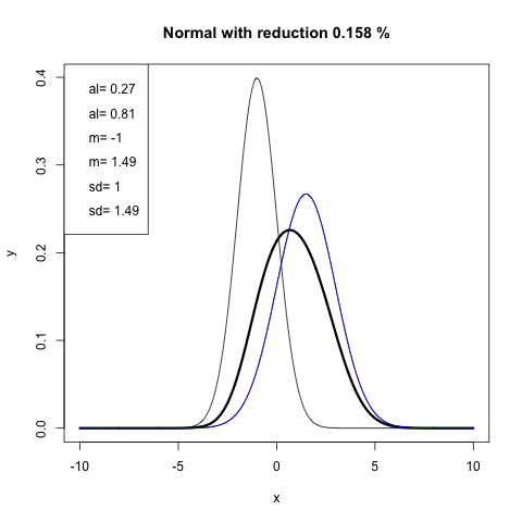
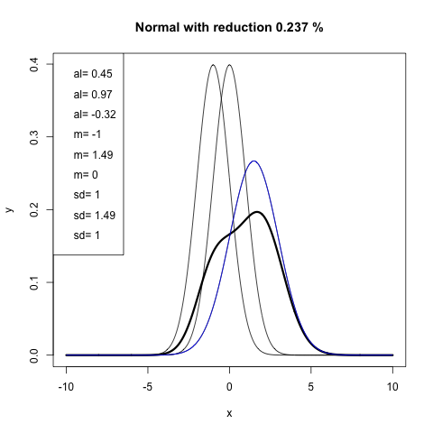
Similar plots are also obtained for the beta distributions (See Figure Figure 5 of Appendix III in the Supplementary Material).
3.2 Example from Ecology
To illustrate the proposed approach to combine experts’ opinion, we consider the example in Wongnak et al. 2022. The authors study the survival (in days) of Ixodies ricins ticks under different (controlled) conditions of temperature and humidity. The data set analysed is available in Milne 1950 (Table 16).
As Parametric Survival Model (PSM), the authors chose a Weibull distribution, where they have included in the scale parameter the effects of two covariates, temperature and humidity. That is, for tick and condition , the survival time behaves as follows:
| (3) |
where and represent the temperature and the humidity in the experimental condition , respectively, is a continuous parameter describing the degree of non-linear effects of , is the vector of coefficients and, finally, is the shape parameter of the Weibull density. In other words, the effects of the two covariates (and their interation) are linked to the scale of the Weibull density through . It is not in the scope of this work to discuss any further the model choices described in Wongnak et al. 2022, nor to perform any inference exercise, but only to show how the opinions of the six expects can be combined using the method here proposed.
| 1 | 1 | 5 | 0.30 | 3.73 | 0.73 | 4 | 1 | 5 | 0.30 | 5.19 | 1.00 |
|---|---|---|---|---|---|---|---|---|---|---|---|
| 2 | 25 | 0.30 | 2.29 | 0.52 | 2 | 20 | 0.30 | 3.38 | 1.00 | ||
| 3 | 5 | 0.95 | 4.50 | 0.21 | 3 | 5 | 0.95 | 7.15 | 0.29 | ||
| 4 | 25 | 0.95 | 5.01 | 0.10 | 4 | 20 | 0.80 | 6.31 | 0.47 | ||
| 2 | 1 | 5 | 0.10 | 2.30 | 0.32 | 5 | 1 | 5 | 0.10 | 0.68 | 0.26 |
| 2 | 25 | 0.10 | 1.60 | 0.30 | 2 | 25 | 0.10 | 0.68 | 0.26 | ||
| 3 | 7 | 0.90 | 5.52 | 0.30 | 3 | 5 | 0.95 | 5.90 | 0.17 | ||
| 4 | 20 | 0.90 | 4.09 | 0.52 | 4 | 25 | 0.95 | 5.60 | 0.18 | ||
| 3 | 1 | 5 | 0.10 | 2.69 | 0.81 | 6 | 1 | 5 | 0.10 | 2.05 | 0.73 |
| 2 | 25 | 0.10 | 1.94 | 0.37 | 2 | 25 | 0.10 | 0.57 | 0.69 | ||
| 3 | 5 | 0.95 | 5.72 | 0.16 | 3 | 8 | 0.95 | 4.79 | 0.25 | ||
| 4 | 20 | 0.95 | 5.90 | 0.05 | 4 | 25 | 0.95 | 2.89 | 0.43 |
The opinions of six experts on the average survival time have been collected, processed and, for each one of them, the believes have been represented by a Log-normal density with given location and scale parameters. The process to transform prior information (i.e. opinion) into suitable density distributions is discussed in the detail in Wongnak et al. 2022 and we refer the reader to it. In short, each expert was asked to provide an informed “guess” of the mean survival time, the highest and the lowest survival time and, finally, how confident they were about their “guesses”. The information, through a suitable software (and some revision activities) was then transformed in the parameters of the log normal density representing their uncertainty. As such, for expert and experimental condition , the average survival time had the following distribution: where and where the location and scale parameter, respectively, of the Log-normal density determined above.

In Wongnak et al. 2022 the aggregation of the experts’ opinions was performed at the level of the induced priors on . Without questioning this approach, as our aim is to illustrate the aggregation process only, we decided to aggregate at the root of the model. In other words, as the prior information was used to formulate a prior distribution on the (mean) survival time, we have combined the information contained in the log-normal densities. The parameters for the log-normal densities are contained in Table 1.
In Figure 4 we have included, for each condition, the resulting density obtained by combining the experts’ opinions, represented by normal densities. We have chosen to not represent the aggregation in the log scale so to have a better visual representation of the differences between our aggregation method and the resulting density one would select if the information was maximized. It is clear the the proposed method results in a wider representation of the experts’ opinions, and the resulting combined densities (for each condition) assign more mass to the region where, overall, the curves representing the experts’ opinions are more dense. This is particularly obvious for Conditions 1 and 2. Interestingly, in Condition 3, we note that the combined density is bimodal, hence capable to incorporate the opinion of the expert represented by the density to the far right. Although less prominent, the same happens for Condition 4.
References
- Albert et. al (2012) Albert, D., Donnet, S., Guihenneuc-Jouyaux, C., Low-Choy, A. Mengersen, K, and Rousseau, J. (2012). Combining Expert Opinions in Prior Elicitation. Bayesian Analysis, 7(3), 503–532.
- Amari (1985) Amari, S. (1985). Differential-geometrical methods in statistics, Lecture Notes in Statistics. 28 Springer- Verlag, New York.
- Bercher and Vignat (2009) Bercher, J.F. and Vignat, C. (2009). On minimum Fisher information distributions with restricted support and fixed variance. Information Sciences, 179(22), 3832–3842.
- Dietrich and List (2016) Dietrich, F. and List, C. (2016). Probabilistic Opinion Pooling. The Oxford Handbook of Probability and Philosophy. (Hajek, A. and Hitchcock, C. Eds.)
- Farr et al. (2018) Farr, C., Ruggeri, F. and Mengersen, K. (2018). Prior and posterior linear pooling for combining expert opinions: uses and impact on Bayesian networks – the case of wayfinding model. Entropy, 20, 209.
- Genest (1983) Genest, C. (1983). Towards a consensus of opinion. Doctoral Dissertation, University of British Columbia.
- Genest and Zidek (1986) Genest, C. and Zidek, J. V. (1986). Combining probability distributions. A critique and annotated bibliography. Statistical Science, 1, 114–148.
- Horn and Johnson (2012) Horn, A. R. and Johnson, C.R. (2012). Matrix Analysis 2d Ed Cambridge University Press.
- Jaynes (1957) Jaynes, E.T. (1957). Information theory and statistical mechanics. Physical Review 106, 620–630.
- Kurtek and Bharath (2015) Kurtek, S. and Bharath, K. (2015). Bayesian sensitivity analysis with the Fisher-Rao metric. Biometrika, 102(3),601–616.
- McConway (1978) McConway, K.J. (1978). The combination of experts’ opinion in probability assessment: some theoretical considerations. Doctoral Dissertation, University College London.
- McConway (1981) McConway, K.J. (1981). Marginalization and linear opinion pools. Journal of the American Statistical Association, 76, 410–414.
- Milne (1950) Milne, A. (1950). The ecology of the sheep tick, Ixodes ricinus L.: Microhabitat economy of the adult tick. Parasitology, 40, 14–-34.
- Saha et al. (2020) A. Saha, K. Bharath and S. Kurtek. (2020). A Geometric Variational Approach to Bayesian Inference. Journal of the American Statistical Association, 115, 822–835.
- Uhrman-Klingen (1995) Uhrmann-Klingen, E. (1995). Minimal Fisher Information Distributions with Compact-Supports. Sankhyā: The Indian Journal of Statistics, Series A, 57(3), 360–374.
- Wongnak et al. (2022) Wongnak, Prustsamon and Bord, Severine and Donnet, Sophie and Hoch, Thierry and Beugnet, Frederic and Chalvet-Monfray, Karine (2022). A hierarchical Bayesian approach for incorporating expert opinions into parametric survival models: A case study of female Ixodies ricins ticks exposed to various temperature and relative humidity conditions. Ecological Modelling, 464, 109821.
Supplementary material
Appendix I
and entries for exponential family components
For the general exponential family parameterization:
and for a pair and we could write
and
These indicate that it is possible to explicitly obtain entries of matrices and where the prior distributions are from the common candidates such as beta, normal, gamma, inverse gamma densities. We report in the following these pairwise entries explicitly.
Appendix II
Calculations for normal densities
For any two particular normal densities
and by completing the relevant quadratic terms
for and . This leads to
| (4) |
Similar calculations for show that
| (5) |
Appendix III
Calculations for Beta densities
For the distribution
and
Then it is possible to show that
and
See Figure 5 for some examples for beta densities using these calculations.


Appendix IV
Calculations for the gamma distributions
The parameterization of the gamma distribution as leads to
Therefore
and
For the exponential densities with parameterization as the gamma distribution above with , then and