Dynamic 3D Scene Analysis by
Point Cloud Accumulation

Our proposed method differs from WsRSF in several ways: (i) WsRSF is a pair-wise scene flow estimation method, while we can handle multiple frames; (ii) unlike WsRSF we perform motion segmentation for a more complete understanding of the scene dynamics; (iii) our method outputs instance-level associations, while WsRSF simply connects each instance to the complete foreground of the other point cloud.

Similar to our method, MotionNet also deals with sequential point clouds and uses a BEV representation. However, MotionNet (i) assumes that ground truth ego-motion is available, while we estimate it within our network; and (ii) does not provide object-level understanding, rather it only separates the scene into a static and a dynamic part.

The Waymo Open Dataset [50] includes 798/202 scenes for training/validation, where each scene is a 20-second clip captured by a 64-beam LiDAR at 10 Hz. We randomly sample 573/201 scenes for training/validation from the training split, and treat the whole validation split as a held-out test set. We consider every 5 consecutive frames as a sample and extract 20 samples from each clip, for a total of 11440/4013/4031 samples for training/validation/test.

The nuScenes dataset [7] consists of 700 training and 150 validation scenes, where each scene is a 20-second clip captured by a 32-beam LiDAR at 20 Hz. We use all validation scenes for testing and randomly hold out 150 training scenes for validation. We consider every 11 consecutive frames as a sample, resulting in a total of 10921/2973/2973 samples for training/validation/testing.

We follow [26] to construct pseudo ground-truth from the detection and tracking annotations. Specifically, the flow vectors of the background part are obtained from ground truth ego-motion. For foreground objects, we use the unique instance IDs of the tracking annotations and recover their rigid motion parameters by registering the bounding boxes. Notably, for nuScenes the bounding boxes are only annotated every 10 frames. To obtain pseudo ground truth for the remaining frames, we linearly interpolate the boxes, which may introduce a small amount of label noise especially for fast-moving objects.

We use standard scene flow evaluation metrics [35, 2] to compare the performance of our approach to the selected baselines. These metric include: (i) 3D end-point-error (EPE [m]) which denotes the mean $L_{2}$-error of all flow vectors averaged over all frames; (ii) strict/relaxed accuracy (AccS [%] /AccR [%]). i.e., the fraction of points with EPE $<$ 0.05/0.10m or relative error $<$ 0.05/0.10; (iii) Outliers [%] which denotes the ratio of points with EPE $>$ 0.30m or relative error $>$ 0.10; and (iv) ROutliers [%], the fraction of points whose EPE $>$ 0.30m and relative error $>$ 0.30. We evaluate these metrics for the static and dynamic parts of the scene separately.²² 2 A point is labelled as dynamic if its ground-truth velocity is $>0.5\,$m/s. Following [62, 38], we evaluate the performance of all methods only on the points that lie within the square of size $64\times 64$ m² centered at the ego-car location in the target frame. Additionally we remove ground points by thresholding along the $z$-axis.³³ 3 This setting turns out to better suit the baseline methods [44, 63, 34]. However, we keep ground points in our dynamic point cloud accumulation task, as thresholding could falsely remove points that are of interest for reconstruction or mapping. Ablations studies additionally report the quality of motion segmentation in terms of recall and precision of dynamic parts, and the quality of spatio-temporal instance association in terms of mean weighted coverage (mWCov, the IoU of recovered instances [59]). For further details, see the supplementary material.

We compare our method to 4 baseline methods. PPWC [63] and FLOT [44] are based on dense matching and are trained in a fully supervised manner; WsRSF [19] assumes a multi-body scene and can be trained with weak supervision; NSFPrior [34] is an optimisation-based method without pre-training. For PPWC [63], FLOT [44] and WsRSF [19], we sample at most 8192 points from each frame due to memory constraints, and use the $k$-nn graph to up-sample flow vectors to full resolution at inference time. For NSFPrior [34], we use the full point clouds and take the default hyper-parameter settings given by the authors, except for the early-stopping patience, which we set to 50 to make it computationally tractable on our large-scale dataset. For all baseline methods, we directly estimate flow vectors from any source frame to the target frame.

On the static part of the Waymo dataset, FLOT [44] reaches the best performance among the baselines, but still has an average EPE error of 12.9 cm, which is more than 4 times larger than that of Ours (2.8 cm). This result corroborates our motivation for decomposing the scene into a static background and dynamic foreground. Modeling the motion of the background with a single set of transformation parameters also enables us to run ICP at test time (Ours+), which further reduces the EPE of the static part to 1.8 cm. On the dynamic foreground points, NSFPrior [34] reaches a comparable performance to Ours. However, based on our spatio-temporal association of foreground points we can again run ICP at test-time, which reduces the median EPE error to 4.3 cm, $\approx$40$\,\%$ lower than that of NSFPrior. Furthermore, NSFPrior is an optimization method and not amenable to online processing (see Tab. 3). The results for nuScenes follow a similar trend as the ones for Waymo, but are larger in absolute terms due to the lower point density. Our method achieves the best performance on both static and dynamic parts. The gap to the closest competitors is even larger, which auggests that our method is more robust to low point density.

To further understand the error distribution of the dynamic parts, and the evolution of the errors of the static part as the gap between the source and target frames increases, we plot detailed results in fig. 3. On both Waymo and nuScenes our method degrades gracefully, and slower than the baselines. The ECDF curve of the EPE error for foreground points also shows that our method performs best at all thresholds.

Overall, our method improves over baseline methods by a large margin on two datasets. The gains are a direct result of our design choices: (i) by modelling the flow of the background as rigid motion instead of unconstrained flow, we can greatly reduce ROutlier and improve the accuracy; (ii) different from [19] we perform motion segmentation, and can thus assign ego-motion flow to points on movable, but static objects ($\approx 75\%$ of the foreground). This further improves the results (see EPE of static FG in table 4); (iii) reasoning on the object level, combined with spatio-temporal association and modelling, improves flow estimates for the dynamic foreground.

When trained with a fixed input length ($T=5$ on Waymo), our model is able to generalize to different input lengths (see Tab. 2). The performance degrades moderately with increasing $T$, as the motions become larger than seen during training. Also, larger displacements make the correspondence problem inherently harder.

We report runtimes for our model and several baseline methods on both datasets in table 3 (left). Our method is significantly faster than all baselines under the multi-frame scene flow setting. We also report detailed runtimes of our model for individual steps in table 3 (right). As we can see, backbone feature extraction and pairwise registration (ego-motion estimation) account for the majority of the runtime, 57.5% on Waymo and 75.2% on nuScenes. Note that this runtime is calculated over all frames, while under a data streaming setting, we only need to run the first part for a single incoming frame, then re-use the features of the previous frames at later stages, which will greatly reduce runtime: after initialisation, the runtime for every new sample decreases to around 0.094 s for Waymo, respectively 0.079 s on nuScenes.

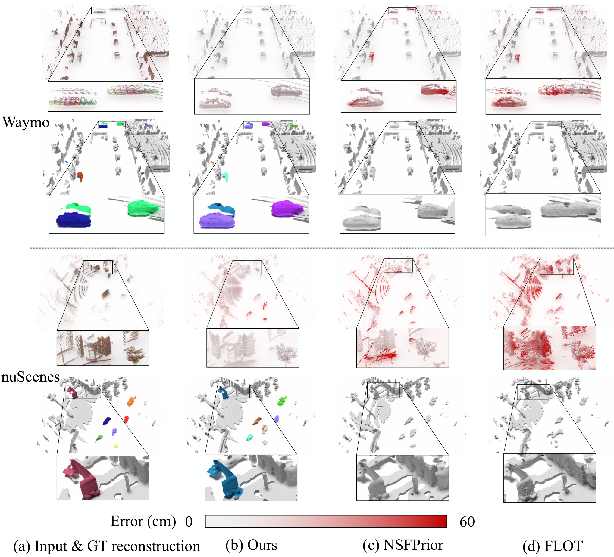
In fig. 4 we show qualitative examples of scene and object reconstruction with our approach. By jointly estimating the ego-motion of the static part and the moving object motions, our method accumulates the corresponding points into a common, motion-compensated frame. It thus provides an excellent basis for 3D surface reconstruction.

We evaluate the individual modules of our sequential model, namely the foreground segmentation (FG), motion segmentation (MOS) and offset compensation (Offset). We train two models with and without foreground segmentation. For variants without MOS or Offset, we take the trained full model but remove MOS or Offset at inference time. The detailed results are summarised in table 4. FG enables us to exclude dynamic foreground objects during pairwise registration. On Waymo, this reduces EPE of the static parts by $30\%$ from 4.1 to 2.9 cm, and as a result also reduces EPE of dynamic parts from 28.6 to 19.7 cm. By additionally extracting the static foreground parts with MOS, the model can recover more accurate ego-motion for them, which reduces EPE from 19.0/19.9 to 2.1/7.4 cm on Waymo/nuScenes. Offset robustifies the instance association against low point density and fast object motion (+3.1 $pp$ in WCov on nuScenes), this further reduces the EPE of dynamic parts by 3.7 cm.

By default, we directly estimate the ego-motion from any source frame to the target frame. We compare to an alternative which estimates the ego-motion relative to the previous frame. Although that achieves smaller pairwise errors, after chaining the estimated poses the errors w.r.t. the target frame explode, resulting in inferior scene flow estimates (chained poses in table 4).

Instead of running spatio-temporal association followed by TubeNet to model the motion of each moving object, an alternative would be to apply Kalman tracker so as to simultaneously solve association and motion. We compare to the modified AB3DMOT [61], which is based on a constant velocity model. That method first clusters moving points for each frame independently to obtain instances, then associates instances by greedy matching of instance centroids based on $L_{2}$ distances. The results in table 4 (Kalman tracker) show clearly weaker performance, due to the less robust proximity metric based on distances between noisy centroid estimates.

To compensate for class imbalance, we use a weighted BCE and compute the weights of each class on the fly. Specifically, for a mini-batch with $N_{\text{pos}}$ positive and $N_{\text{neg}}$ negative samples, the associated weights $w_{\text{pos}}$ and $w_{\text{neg}}$ are computed as:

$$w_{\text{pos}}=\min(\sqrt{\frac{N_{\text{pos}}+N_{\text{neg}}}{N_{\text{pos}}}},w_{\text{max}})\qquad w_{\text{neg}}=\min(\sqrt{\frac{N_{\text{pos}}+N_{\text{neg}}}{N_{\text{neg}}}},w_{\text{max}})\;,$$

(13)

where $w_{\text{max}}$ is the maximum weight of a class.⁶⁶ 6 We find that in some extreme cases, there are very few ($<10$) positive samples and way more negative samples. We thus bound $w_{\text{max}}$ at 50 to ensure stability. The final weighted BCE loss $\mathcal{L}_{\mathrm{bce}}(\mathbf{x},\overline{\mathbf{x}})$ is

$$\mathcal{L}_{\mathrm{bce}}(\mathbf{x},\overline{\mathbf{x}})\!=\frac{1}{|\mathbf{x}|}\sum_{i=1}^{|\mathbf{x}|}w_{i}(\overline{\mathbf{x}}_{i}\log(\mathbf{x}_{i})+(1-\overline{\mathbf{x}}_{i})\log(1-\mathbf{x}_{i}))\;,$$

(14)

with $\mathbf{x}$ and $\overline{\mathbf{x}}$ are predicted and ground truth labels, and $w_{i}$ the weight of the $i^{\text{th}}$ sample, computed as

$$w_{i}=\begin{cases}w_{\text{pos.}},&\text{if }\overline{\mathbf{x}}_{i}=1\\ w_{\text{neg.}},&\text{otherwise}\end{cases}\;.$$

(15)

The Jaccard index (ratio of Intersection over Union) is commonly used to measure segmentation quality. In the binary classification setting, we can set the ground truth labels as $\overline{\mathbf{x}}_{i}\in\{-1,1\}$, then the Jaccard index of the foreground class $J_{1}$ is computed as

$$J_{1}(\overline{\mathbf{x}},\mathbf{x})=\frac{|\{\overline{\mathbf{x}}=1\}\cap\{\mathrm{sign}(\mathbf{x})=1\}|}{|\{\overline{\mathbf{x}}=1\}\cup\{\mathrm{sign}(\mathbf{x})=1\}|}\;,\quad J_{1}(\overline{\mathbf{x}},\mathbf{x})\in[0,1]\;,$$

(16)

with $\mathbf{x}$ the prediction and $\mathrm{sign}()$ the sign function. The corresponding loss $\Delta_{J_{1}}(\overline{\mathbf{x}},\mathbf{x})$ to minimise the empirical risk is

$$\Delta_{J_{1}}(\overline{\mathbf{x}},\mathbf{x})=1-J_{1}(\overline{\mathbf{x}},\mathbf{x})\;.$$

(17)

However, this is not differentiable and cannot be directly employed as a loss function. The authors of [5] have proposed to optimise it using a Lovász extension. The Lovász extension $\dddot{\Delta}$ of a set function $\Delta$ is defined as:

$$\dddot{\Delta}(\mathbf{m})=\sum_{i=1}^{p}\mathbf{m}_{i}\,g_{i}(\mathbf{m})\;,$$

(18)

with

$$g_{i}(\mathbf{m})=\Delta(\{\pi_{1},\ldots,\pi_{i}\})-\Delta(\{\pi_{1},\ldots,\pi_{i-1}\}),$$

(19)

where $\mathbf{\pi}$ denotes a permutation that places the components of $\mathbf{m}$ in decreasing order. Considering $\mathbf{m}_{i}=\max(1-\mathbf{x}_{i}\overline{\mathbf{x}}_{i},0)$, the Lovász-Softmax loss $\mathcal{L}_{ls}(\overline{\mathbf{x}},\mathbf{x})$ is defined as

$$\mathcal{L}_{ls}(\overline{\mathbf{x}},\mathbf{x})=\dddot{\Delta_{J_{1}}}(\mathbf{m}).$$

(20)

Previous works [66, 19] have observed that the entropy-regularized optimal transport [11] has a tendency to label most points as outliers. To alleviate this issue, we follow [66, 19] and use an inlier loss $\mathcal{L}_{\text{inlier}}$ on the matching matrix $\mathbf{D}^{t}$, designed to encourage inliers. The inlier loss is defined as

$$\mathcal{L}_{\text{inlier}}^{t}=\frac{1}{2N_{\mathrm{ego}}}(2N_{\mathrm{ego}}-\sum_{l=1}^{N_{\mathrm{ego}}}\sum_{m=1}^{N_{\mathrm{ego}}}\mathbf{D}_{l,m}^{t})\;.$$

(21)

To quantitatively measure the spatio-temporal instance association quality, we report weighted coverage (WCov) as well as recall and precision at a certain threshold. Given the ground truth clusters $\mathcal{G}$ and the estimated clusters $\mathcal{O}$, recall measures the ratio of clusters in $\mathcal{G}$ that have an overlap above some threshold with a cluster in $\mathcal{O}$, while precision does the same in the opposite direction. Weighted coverage $WCov(\mathcal{G},\mathcal{O})$ is computed as

$$WCov(\mathcal{G},\mathcal{O})=\sum_{i=1}^{|\mathcal{G}|}\frac{1}{|\mathcal{G}|}w_{i}\max_{j}\mathrm{IoU}(r_{i}^{G},r_{j}^{0}),\qquad w_{i}=\frac{|r_{i}^{G}|}{\sum_{k}|r_{k}^{G}|}\;,$$

(22)

where $r_{i}^{G}$ and $r_{j}^{O}$ are clusters from $\mathcal{G}$ and $\mathcal{O}$, and $\mathrm{IoU}(r_{i}^{G},r_{j}^{O})$ denotes the overlap between two clusters.

The Empirical Cumulative Distribution Function (ECDF) measures the distribution of a set of values:

$\displaystyle\text{ECDF}(x)=\frac{\big|\{o_{i}<x\}\big|}{\big|O\big|}\;,$

(23)

where $O=\{o_{i}\}$ is a set of samples and $x\in[\min\{O\},\max\{O\}]$.

References

- [1] Aygun, M., Osep, A., Weber, M., Maximov, M., Stachniss, C., Behley, J., Leal-Taixé, L.: 4d panoptic LiDAR segmentation. In: Proc. CVPR (2021)
- [2] Baur, S.A., Emmerichs, D.J., Moosmann, F., Pinggera, P., Ommer, B., Geiger, A.: SLIM: Self-supervised LiDAR scene flow and motion segmentation. In: Proc. ICCV (2021)
- [3] Behl, A., Paschalidou, D., Donné, S., Geiger, A.: PointFlowNet: Learning representations for rigid motion estimation from point clouds. In: Proc. CVPR (2019)
- [4] Behley, J., Garbade, M., Milioto, A., Quenzel, J., Behnke, S., Stachniss, C., Gall, J.: SemanticKITTI: A dataset for semantic scene understanding of lidar sequences. In: Proc. ICCV (2019)
- [5] Berman, M., Triki, A.R., Blaschko, M.B.: The Lovász-Softmax loss: A tractable surrogate for the optimization of the intersection-over-union measure in neural networks. In: Proc. CVPR (2018)
- [6] Besl, P.J., McKay, N.D.: Method for registration of 3-d shapes. In: Sensor fusion IV: control paradigms and data structures. vol. 1611, pp. 586–606. International Society for Optics and Photonics (1992)
- [7] Caesar, H., Bankiti, V., Lang, A.H., Vora, S., Liong, V.E., Xu, Q., Krishnan, A., Pan, Y., Baldan, G., Beijbom, O.: nuScenes: A multimodal dataset for autonomous driving. In: Proc. CVPR (2020)
- [8] Chen, C., Yang, B.: Dynamic occlusion detection and inpainting of in situ captured terrestrial laser scanning point clouds sequence. ISPRS Journal of Photogrammetry and Remote Sensing 119, 90–107 (2016)
- [9] Chen, X., Li, S., Mersch, B., Wiesmann, L., Gall, J., Behley, J., Stachniss, C.: Moving object segmentation in 3D LiDAR data: A learning-based approach exploiting sequential data. IEEE RA-L (2021)
- [10] Choy, C., Gwak, J., Savarese, S.: 4d spatio-temporal convnets: Minkowski convolutional neural networks. In: Proc. CVPR (2019)
- [11] Cuturi, M.: Sinkhorn distances: Lightspeed computation of optimal transport. Proc. NeurIPS (2013)
- [12] Dendorfer, P., Osep, A., Milan, A., Schindler, K., Cremers, D., Reid, I., Roth, S., Leal-Taixé, L.: MOTchallenge: A benchmark for single-camera multiple target tracking. IJCV (2021)
- [13] Dewan, A., Caselitz, T., Tipaldi, G.D., Burgard, W.: Rigid scene flow for 3d lidar scans. In: Proc. IROS (2016)
- [14] Ester, M., Kriegel, H.P., Sander, J., Xu, X., et al.: A density-based algorithm for discovering clusters in large spatial databases with noise. In: Proc. KDD (1996)
- [15] Fan, H., Yang, Y., Kankanhalli, M.: Point 4d transformer networks for spatio-temporal modeling in point cloud videos. In: Proc. CVPR (2021)
- [16] Fan, H., Yu, X., Ding, Y., Yang, Y., Kankanhalli, M.: PSTNet: Point spatio-temporal convolution on point cloud sequences. In: Proc. ICLR (2020)
- [17] Filatov, A., Rykov, A., Murashkin, V.: Any motion detector: Learning class-agnostic scene dynamics from a sequence of lidar point clouds. In: Proc. ICRA (2020)
- [18] Giancola, S., Zarzar, J., Ghanem, B.: Leveraging shape completion for 3d siamese tracking. In: Proc. CVPR (2019)
- [19] Gojcic, Z., Litany, O., Wieser, A., Guibas, L.J., Birdal, T.: Weakly supervised learning of rigid 3d scene flow. In: Proc. CVPR (2021)
- [20] Gojcic, Z., Zhou, C., Wegner, J.D., Guibas, L.J., Birdal, T.: Learning multiview 3d point cloud registration. In: Proc. CVPR (2020)
- [21] Groß, J., Ošep, A., Leibe, B.: AlignNet-3D: Fast point cloud registration of partially observed objects. In: Proc. 3DV (2019)
- [22] Gu, J., Ma, W.C., Manivasagam, S., Zeng, W., Wang, Z., Xiong, Y., Su, H., Urtasun, R.: Weakly-supervised 3d shape completion in the wild. In: Proc. ECCV (2020)
- [23] Huang, J., Birdal, T., Gojcic, Z., Guibas, L.J., Hu, S.M.: Multiway non-rigid point cloud registration via learned functional map synchronization. IEEE T-PAMI (2022)
- [24] Huang, J., Wang, H., Birdal, T., Sung, M., Arrigoni, F., Hu, S.M., Guibas, L.J.: MultiBodySync: Multi-body segmentation and motion estimation via 3d scan synchronization. In: Proc. CVPR (2021)
- [25] Ioffe, S., Szegedy, C.: Batch normalization: Accelerating deep network training by reducing internal covariate shift. In: Proc. ICML (2015)
- [26] Jund, P., Sweeney, C., Abdo, N., Chen, Z., Shlens, J.: Scalable scene flow from point clouds in the real world. arXiv preprint arXiv:2103.01306 (2021)
- [27] Kabsch, W.: A solution for the best rotation to relate two sets of vectors. Acta Crystallographica Section A: Crystal Physics, Diffraction, Theoretical and General Crystallography 32(5), 922–923 (1976)
- [28] Kazhdan, M., Bolitho, M., Hoppe, H.: Poisson surface reconstruction. In: Eurographics (2006)
- [29] Kim, G., Kim, A.: Remove, then revert: Static point cloud map construction using multiresolution range images. In: Proc. IROS (2020)
- [30] Kingma, D.P., Ba, J.: Adam: A method for stochastic optimization. arXiv preprint arXiv:1412.6980 (2014)
- [31] Lahoud, J., Ghanem, B., Pollefeys, M., Oswald, M.R.: 3d instance segmentation via multi-task metric learning. In: Proc. ICCV (2019)
- [32] Li, R., Lin, G., He, T., Liu, F., Shen, C.: HCRF-Flow: Scene flow from point clouds with continuous high-order crfs and position-aware flow embedding. In: Proc. CVPR (2021)
- [33] Li, R., Li, X., Fu, C.W., Cohen-Or, D., Heng, P.A.: PU-GAN: a point cloud upsampling adversarial network. In: Proc. ICCV (2019)
- [34] Li, X., Kaesemodel Pontes, J., Lucey, S.: Neural scene flow prior. Proc. NeurIPS (2021)
- [35] Liu, X., Qi, C.R., Guibas, L.J.: FlowNet3D: Learning scene flow in 3d point clouds. In: Proc. CVPR (2019)
- [36] Liu, X., Yan, M., Bohg, J.: Meteornet: Deep learning on dynamic 3d point cloud sequences. In: Proc. ICCV (2019)
- [37] Long, J., Shelhamer, E., Darrell, T.: Fully convolutional networks for semantic segmentation. In: Proc. CVPR (2015)
- [38] Luo, C., Yang, X., Yuille, A.: Self-supervised pillar motion learning for autonomous driving. In: Proc. CVPR (2021)
- [39] Ouyang, B., Raviv, D.: Occlusion guided self-supervised scene flow estimation on 3d point clouds. arXiv preprint arXiv:2104.04724 (2021)
- [40] Paszke, A., Gross, S., Massa, F., Lerer, A., Bradbury, J., Chanan, G., Killeen, T., Lin, Z., Gimelshein, N., Antiga, L., Desmaison, A., Kopf, A., Yang, E., DeVito, Z., Raison, M., Tejani, A., Chilamkurthy, S., Steiner, B., Fang, L., Bai, J., Chintala, S.: Pytorch: An imperative style, high-performance deep learning library. Proc. NeurIPS (2021)
- [41] Peng, S., Niemeyer, M., Mescheder, L., Pollefeys, M., Geiger, A.: Convolutional occupancy networks. In: Proc. ECCV (2020)
- [42] Piergiovanni, A., Casser, V., Ryoo, M.S., Angelova, A.: 4d-net for learned multi-modal alignment. arXiv preprint arXiv:2109.01066 (2021)
- [43] Pomerleau, F., Krüsi, P., Colas, F., Furgale, P., Siegwart, R.: Long-term 3d map maintenance in dynamic environments. In: Proc. ICRA (2014)
- [44] Puy, G., Boulch, A., Marlet, R.: FLOT: Scene flow on point clouds guided by optimal transport. In: Proc. ECCV (2020)
- [45] Qi, C.R., Su, H., Mo, K., Guibas, L.J.: Pointnet: Deep learning on point sets for 3d classification and segmentation. In: Proc. CVPR (2017)
- [46] Qi, C.R., Zhou, Y., Najibi, M., Sun, P., Vo, K., Deng, B., Anguelov, D.: Offboard 3d object detection from point cloud sequences. In: Proc. CVPR (2021)
- [47] Rempe, D., Birdal, T., Zhao, Y., Gojcic, Z., Sridhar, S., Guibas, L.J.: CaSPR: Learning canonical spatiotemporal point cloud representations. In: Proc. NeurIPS (2020)
- [48] Schauer, J., Nüchter, A.: The peopleremover—removing dynamic objects from 3-d point cloud data by traversing a voxel occupancy grid. IEEE RA-L 3(3), 1679–1686 (2018)
- [49] Sun, D., Yang, X., Liu, M.Y., Kautz, J.: PWC-net: Cnns for optical flow using pyramid, warping, and cost volume. In: Proc. CVPR (2018)
- [50] Sun, P., Kretzschmar, H., Dotiwalla, X., Chouard, A., Patnaik, V., Tsui, P., Guo, J., Zhou, Y., Chai, Y., Caine, B., et al.: Scalability in perception for autonomous driving: Waymo open dataset. In: Proc. CVPR (2020)
- [51] Tang, H., Liu, Z., Li, X., Lin, Y., Han, S.: TorchSparse: Efficient Point Cloud Inference Engine. In: MLSys (2022)
- [52] Teed, Z., Deng, J.: RAFT-3D: Scene flow using rigid-motion embeddings. In: Proc. CVPR (2021)
- [53] Vaswani, A., Shazeer, N., Parmar, N., Uszkoreit, J., Jones, L., Gomez, A.N., Kaiser, Ł., Polosukhin, I.: Attention is all you need. In: Proc. NeurIPS (2017)
- [54] Vedula, S., Baker, S., Rander, P., Collins, R., Kanade, T.: Three-dimensional scene flow. In: Proc. ICCV (1999)
- [55] Vogel, C., Schindler, K., Roth, S.: 3d scene flow estimation with a rigid motion prior. In: Proc. ICCV (2011)
- [56] Vogel, C., Schindler, K., Roth, S.: Piecewise rigid scene flow. In: Proc. ICCV (2013)
- [57] Vogel, C., Schindler, K., Roth, S.: 3d scene flow estimation with a piecewise rigid scene model. International Journal of Computer Vision 115(1), 1–28 (2015)
- [58] Wang, H., Sridhar, S., Huang, J., Valentin, J., Song, S., Guibas, L.J.: Normalized object coordinate space for category-level 6d object pose and size estimation. In: Proc. CVPR (2019)
- [59] Wang, X., Liu, S., Shen, X., Shen, C., Jia, J.: Associatively segmenting instances and semantics in point clouds. In: Proc. CVPR (2019)
- [60] Wedel, A., Rabe, C., Vaudrey, T., Brox, T., Franke, U., Cremers, D.: Efficient dense scene flow from sparse or dense stereo data. In: Proc. ECCV (2008)
- [61] Weng, X., Wang, J., Held, D., Kitani, K.: 3d multi-object tracking: A baseline and new evaluation metrics. In: Proc. IROS (2020)
- [62] Wu, P., Chen, S., Metaxas, D.N.: MotionNet: Joint perception and motion prediction for autonomous driving based on bird’s eye view maps. In: Proc. CVPR (2020)
- [63] Wu, W., Wang, Z.Y., Li, Z., Liu, W., Fuxin, L.: Pointpwc-net: Cost volume on point clouds for (self-) supervised scene flow estimation. In: Proc. ECCV (2020)
- [64] Yang, B., Bai, M., Liang, M., Zeng, W., Urtasun, R.: Auto4d: Learning to label 4d objects from sequential point clouds. arXiv preprint arXiv:2101.06586 (2021)
- [65] Yang, Z., Zhou, Y., Chen, Z., Ngiam, J.: 3D-MAN: 3d multi-frame attention network for object detection. In: Proc. CVPR (2021)
- [66] Yew, Z.J., Lee, G.H.: RPM-Net: Robust point matching using learned features. In: Proc. CVPR (2020)
- [67] Yuan, W., Khot, T., Held, D., Mertz, C., Hebert, M.: PCN: Point completion network. In: Proc. 3DV (2018)
- [68] Zhou, Q.Y., Park, J., Koltun, V.: Open3D: A modern library for 3D data processing. arXiv preprint arXiv:1801.09847 (2018)
In this supplementary document, we first present additional information about our network architecture and implementation in section A. We then elaborate on technical details of ego-motion estimation, iterative pose refinement, and scene reconstruction in section B. Precise definitions of loss functions and evaluation metrics are provided in section C. Further analysis of the two datasets, nuScenes and Waymo, is presented in section D, followed by additional quantitative results including scene flow estimation, instance association, and the TubeNet motion model in section E. Finally, we show more qualitative results in section F.
A Network and implementation
Network architecture
The detailed network architecture is depicted in fig. 10. Our network is a sequential model consisting of (i) per-frame feature extraction used to estimate ego-motion, (ii) multi-frame feature extraction to segment dynamic objects and regress offset vectors towards the associated instance center, and (iii) TubeNet to regress the rigid motions of dynamic objects. The Pillar encoder and the two UNets operate without Batch Normalisation [25], this speeds up training and inference without any loss in performance [41]. Our network achieves flexibility w.r.t. the number of input frames via global max-pooling along the temporal dimension in the InitConv3D block (fig. 10).
Implementation details
We use torch_scatter44 4 https://github.com/rusty1s/pytorch_scatter to efficiently convert point-wise features to pillar/instance-level global features. To spatially align the backbone features we use grid_sample, implemented in PyTorch [40]. Before clustering, we apply voxel down-sampling implemented in TorchSparse [51] to reduce the point density and improve clustering efficiency. The voxel size is set to 15 cm. Instance labels at full resolution are recovered by indexing points to their associated voxel cell.
B Methodology
Ego-motion estimation
Given two sets of pillar centroid coordinates and associated -normalised features , we first compute the cost matrix and an Euclidean distance matrix from pillar coordinates. We then pad with a learnable slack row and column to accommodate outliers, before iteratively alternating between row normalisation and column normalisation55 5 To improve training stability, row and column normalisations operate in -space. for five times to approximate a doubly stochastic permutation matrix that satisfies