dCAM: Dimension-wise Class Activation Map
for Explaining Multivariate Data Series ClassificationConference: Proceedings of the 2022 International Conference on Management of Data; June 12–17, 2022; Philadelphia, PA, USAProceedings of the 2022 International Conference on Management of Data (SIGMOD ’22), June 12–17, 2022, Philadelphia, PA, USAPrice: 15.00DOI: 10.1145/3514221.3526183ISBN: 978-1-4503-9249-5/22/06
Abstract.
Data series classification is an important and challenging problem in data science. Explaining the classification decisions by finding the discriminant parts of the input that led the algorithm to some decision is a real need in many applications. Convolutional neural networks perform well for the data series classification task; though, the explanations provided by this type of algorithms are poor for the specific case of multivariate data series. Addressing this important limitation is a significant challenge. In this paper, we propose a novel method that solves this problem by highlighting both the temporal and dimensional discriminant information. Our contribution is two-fold: we first describe a convolutional architecture that enables the comparison of dimensions; then, we propose a method that returns dCAM, a Dimension-wise Class Activation Map specifically designed for multivariate time series (and CNN-based models). Experiments with several synthetic and real datasets demonstrate that dCAM is not only more accurate than previous approaches, but the only viable solution for discriminant feature discovery and classification explanation in multivariate time series. This paper has appeared in SIGMOD’22.
1. Introduction
Several applications across many domains produce big collections of data series11 1 A data series, or data sequence, is an ordered sequence of points. If the dimension that imposes the ordering of the sequence is time, then we talk about time series. In this paper, we use the terms sequence, data series, and time series interchangeably., which need to be processed and analyzed (Palpanas 2015; Palpanas 2016; Palpanas and Beckmann 2019; Bagnall et al. 2019). Typical analysis tasks include pattern matching (or similarity search) (Echihabi et al. 2018; Echihabi et al. 2019; Palpanas 2019; Peng et al. 2021b; Gogolou et al. 2020; Peng et al. 2021a; Peng et al. 2021c; Levchenko et al. 2021; Wang and Palpanas 2021; Echihabi et al. 2022), classification (Ye and Keogh 2011; Schäfer and Leser 2017; Lucas et al. 2019; Shifaz et al. 2020; Dempster et al. 2020; Tan et al. 2020; Schäfer and Leser 2020; Ismail Fawaz et al. 2020), clustering (Ulanova et al. 2015; Paparrizos and Gravano 2016; Paparrizos and Gravano 2017; Paparrizos and Franklin 2019; Li et al. 2019), anomaly detection (Paparrizos et al. 2022; Yankov et al. 2008; Boniol and Palpanas 2020; Gao et al. 2020; Boniol et al. 2021a; Boniol et al. 2021b; Schneider et al. 2021), motif discovery (Linardi et al. 2020; Gao and Lin 2019; Zhu et al. 2021), and others (Jakovljevic et al. 2022).
Data series classification is a crucial and challenging problem in data science (Yang and Wu 2006; Esling and Agon 2012). To solve this task, various data series classification algorithms have been proposed in the past few years (Bagnall et al. 2016), applied on a large number of use cases. Standard data series classification methods are based on distances to the instances’ nearest neighbors, with k-NN classification (using the Euclidean or Dynamic Time Warping (DTW) distances) being a popular baseline method (Dau et al. 2019). Nevertheless, recent works have shown that ensemble methods using more advanced classifiers achieve better performance (Bagnall et al. 2015; Lines et al. 2016). Following recent breakthroughs in the computer vision community, new studies successfully propose deep learning methods for data series classification (Ismail Fawaz et al. 2019; Cui et al. 2016; Zheng et al. 2014; Zhao et al. 2017; Le Guennec et al. 2016; Wang et al. 2018; Chen et al. 2013), such as Convolutional Neural Network (CNN), Residual Neural Network (ResNet) (Wang et al. 2017), and InceptionTime (Ismail Fawaz et al. 2020).

[Classification Explanation] While having a trained and accurate classification model, finding explanations of the classification result (i.e., finding the discriminative features that made the model decide which class to attribute to each instance) is a challenging but essential problem, e.g., in manufacturing for anomaly-based predictive maintenance (Zhang et al. 2019), or in medicine for robot-assisted surgeon training (Ismail Fawaz et al. 2018). Such discriminant features can be based on patterns of interest that occur in a subset of dimensions at different timestamps or the same timestamp. For some CNN-based models, the Class Activation Map (CAM) (Zhou et al. 2016) can be used as an explanation for the classification result. CAM has been used for highlighting the parts of an image that contribute the most to a given class prediction and has also been adapted to data series (Ismail Fawaz et al. 2019; Wang et al. 2017).
[Challenges] Nevertheless, CAM for data series suffers from one important limitation. Since CAM is a univariate time series (of the same length as the input instances) with high values aligned with the subsequences of the input that contribute the most for a given class identification, in the specific case of multivariate data series as input, no information can be retrieved from CAM on the level of contribution of specific dimensions. As an example, Figure 1 illustrates CAM (top heatmaps) applied on two instances (belonging to two different classes) of the RacketSport UCR/UEA dataset. We observe that CAM explains why the data series correspond to a badminton "smash" or "clear" gesture by highlighting the same temporal window across all dimensions (variables). It is thus not clear what aspect of the gesture distinguishes it from the other. Addressing this significant limitation is a sought-after challenge.
[Contributions] In this paper, we present a novel approach that fills-in the gap by addressing this limitation for the popular CNN-based models. We propose a novel data organization and a new CAM technique, dCAM (Dimension-wise Class Activation Map), that is able to highlight both the temporal and dimensional information at the same time. For instance, in Figure 1, dCAM (bottom heatmaps) is pointing to specific subsequences of particular dimensions that explain why the two gestures are different. Our method requires only a single training phase, is not constrained by the architecture type, and can efficiently and effectively retrieve discriminant features thanks to a technique that exploits information from different permutations of the input data dimensions. Thus, any kind of architecture in which we can apply CAM can benefit from our approach. Our contributions are as follows.
- •
We develop a new method that transforms convolutional-based neural network architectures: whereas previous network architectures can only provide an explanation for all the dimensions together, our transformation represents the only deep learning solution that enables explanation in individual dimensions. Our approach can be used with any deep network architecture with a Global Average Pooling layer.
- •
We demonstrate how we can apply our method to three modern deep learning classification architectures. We first describe dCNN, inspired by the traditional CNN architecture. We then describe how more advanced architectures, such as ResNet and InceptionTime, can be transformed as well. We name these transformed architectures dResNet and dInceptionTime.
- •
We propose dCAM, a novel method (based on dCNN/ dResNet/dInceptionTime) that returns a multivariate CAM, identifying the important parts of the input series for each dimension.
- •
We experimentally demonstrate with several synthetic and real datasets that (among Class Activation Map-based methods) dCAM is not only more accurate in classification than previous approaches, but the only viable solution for discriminant feature discovery and classification explanation in multivariate time series. Finally, we make our code available online (our 2022).
2. Background and Related Work
We first present useful notations and definitions, and discuss related work. Table 1 summarizes the symbols we use in this paper.
[Data Series] A multivariate, or -dimensional data series is a set of univariate data series of length . We note and for , we note the univariate data series . A subsequence of the dimension of the multivariate data series is a subset of contiguous values from of length (usually ) starting at position ; formally, .
[Neural Network Notations] We are interested in classifying data series using a neural network architecture model. We define the neural network input as for univariate data series (with the value and the sequence of values following the value), and for multivariate data series (with the value on the dimension and the sequence of values following the value on the dimension).
Dense Layer: The basic layer of neural network is a fully connected layer (also called ) in which every input neuron is weighted and summed before passing through an activation function. For univariate data series, given an input data series , given a vector of weights and a vector , we have:
| (1) | ||||
is called the activation function and is a non-linear function. The commonly used activation function is the rectified linear unit (ReLU) (Nair and Hinton 2010) that prevents the saturation of the gradient (other functions that have been proposed are and Leaky (Xu et al. 2015)). For the specific case of multivariate data series, all dimensions are concatenated to give input . Finally, one can decide to have several output neurons. In this case, each neuron is associated with a different and , and Equation 1 is executed independently.
Convolutional Layer: This layer has played a significant role for image classification (Krizhevsky et al. 2012; LeCun et al. 2015; Wang et al. 2017), and recently for data series classification (Ismail Fawaz et al. 2019). Formally, for multivariate data series, given an input vector , and given matrices weights , the output of a convolutional layer can be seen as a univariate data series. The tuple is also called kernel, with the size of the kernel. Formally, for , we have:
| (2) | ||||
In practice, we have several kernels of size . The result is a multivariate series with dimensions equal to the number of kernels, . For a given input , we define to be the output of a convolutional layer . is thus a univariate series corresponding to the output of the kernel. We denote with the univariate series corresponding to the output of the kernel, when is used as input.
Global Average Pooling Layer: Another type of layer frequently used is pooling. Pooling layers compute average/max/min operations, aggregating values of previous layers into a smaller number of values for the next layer. A specific type of pooling layer is Global Average Pooling (GAP). This operation is averaging an entire output of a convolutional layer into one value, thus providing invariance to the position of the discriminative features.
Learning Phase: The learning phase uses a loss function that measures the accuracy of the model and optimizes the various weights. For the sake of simplicity, we note the set containing all weights (e.g., matrices and defined in the previous sections). Given a set of instances , we define the average loss as: . Then for a given learning rate , the average loss is back-propagated to all weights in the different layers. Formally, back-propagation is defined as follows: . In this paper, we use the stochastic gradient descent using the ADAM optimizer (Kingma and Ba 2015) and cross-entropy loss function.
2.1. Convolutional-based Neural Network
We now describe the standard architectures used in the literature. The first is Convolutional Neural Networks (CNNs) (Ismail Fawaz et al. 2019; Wang et al. 2017). CNN is a concatenation of convolutional layers (joined with activation functions and batch normalization). The last convolutional layer is connected to a Global Average Pooling layer and a dense layer. In theory, instances of multiple lengths can be used with the same network. A second architecture is the Residual Neural Network (ResNet) (Ismail Fawaz et al. 2019; Wang et al. 2017). This architecture is based on the classical CNN, to which we add residual connections between successive blocks of convolutional layers to avoid that the gradients explode or vanish. Other methods have been proposed in the literature (Serrà et al. 2018; Ismail Fawaz et al. 2019; Cui et al. 2016; Ismail Fawaz et al. 2020), though, CNN and ResNet have been shown to perform the best for multivariate time series classification (Ismail Fawaz et al. 2019). InceptionTime (Ismail Fawaz et al. 2020) has not been evaluated on multivariate data series, but demonstrated state-of-the-art performance on univariate data series. Finally, other kinds of architectures than convolutional ones have been proposed in the literature. Attention-based models have been introduced, such as TapNet (Zhang et al. 2020). For the specific case of temporal data, recurrent-based models, such as Recurrent Neural Neworks (Rumelhart et al. 1986) (RNN), Long-Short Term Memory (Hochreiter and Schmidhuber 1997) (LSTM), and Gated Recurrent Unit (Cho et al. 2014) (GRU) have received a lot of attention. These three models are relevant to the data series classification task, and we include them in our experimental study.
2.2. Class Activation Map (CAM)
Once the model is trained, we need to find the discriminative features that led the model to decide which class to attribute to each instance. Several methods have been proposed to extract meaningful information from CNNs, such as grad-CAM (Selvaraju et al. 2017) that uses the gradients of the weights to compute the discriminant features, and CAM (Zhou et al. 2016). The latter has been proposed to highlight the parts of an image that contributes the most to a given class identification. The latter has been experimented on data series (Ismail Fawaz et al. 2019; Wang et al. 2017) (univariate and multivariate). This method explains the classification of a certain deep learning model by emphasizing the subsequences that contribute the most to a certain classification. Note that the CAM method can only be used if (i) a Global Average Pooling layer has been used before the classifier, (ii) the model accuracy is high enough. Thus, only the standard architectures CNN and ResNet proposed in the literature can benefit from CAM. We now define the CAM method (Ismail Fawaz et al. 2019; Wang et al. 2017). For an input data series , let be the result of the last convolutional layer , which is a multivariate data series with dimensions and of length . is the univariate time series for the dimension corresponding to the kernel. Let be the weight between the kernel and the output neuron of class . Since a Global Average Pooling layer is used, the input to the neuron of class can be expressed by the following equation:
The second sum represents the averaged time series over the whole time dimension. Note that weight is independent of index . Thus, can also be written by the following equation:
Finally, that underlines the discriminative features of class is defined as follows:
As a consequence, is a univariate data series where each element at index indicates the significance of the index (regardless of the dimensions) for the classification as class . Figure 2(a) depicts the process of computing CAM and finding the discriminant subsequences in the initial series.
2.3. CAM Limitations for Multivariate Series
As mentioned earlier, a CAM that highlights the discriminative subsequences of class , , is a univariate data series. The information provided by is sufficient for the case of univariate series classification, but not for multivariate series classification. Even though the significant temporal index may be correctly highlighted, no information can be retrieved on which dimension is significant or not. Solving this serious limitation is a significant challenge in several domains. For that purpose, one can propose rearranging the input structure to the network so that the CAM becomes a multivariate data series. A new solution would be to decide to use a 2D convolutional neural network with kernel size , such that each kernel slides on each dimension separately. Thus, for an input data series , would become a multivariate data series for the variable , and would be a univariate time series that would correspond to the dimension of the initial data series. We call this solution cCNN, and we use cCAM to refer to the corresponding Class Activation Map. Figure 2(b) illustrates cCNN architecture and cCAM. Note that if a GAP layer is used, then architectures other than CNN can be used, as well, such as ResNet and InceptionTime. We denote these baselines as cResNet and cInceptionTime.
Nevertheless, new limitations arise from this solution. The dimensions are not compared together: each kernel of the input layer will take as input only one of the dimensions at a time. Thus, features depending on more than one dimension will not be detected.
Recent studies study the specific case of multivariate data series classification explanation. A benchmark study analyzing the saliency/explanation methods for multivariate time series concluded that the explainable methods work better when the multivariate data series is handled as an image (Ismail et al. 2020), such as in the cCNN architecture. This confirms the need to propose a method specifically designed for multivariate data series. Finally, some recently proposed approaches (Hsieh et al. 2021; Assaf et al. 2019) address the problems of identifying the discriminant features and discriminant temporal windows independently from one another. For instance, MTEX-CNN (Assaf et al. 2019) is an architecture composed of two blocks. The 1st block is similar to cCNN. The 2nd block consists of merging the results of the 1st block into a 1D convolutional layer, which enables comparing dimensions. A variant of CAM (Selvaraju et al. 2017) is applied to the last convolutional layer of the 1st block in order to find discriminant features for each dimension. The discriminant temporal windows are detected with the CAM applied to the last convolutional layer of the 2nd block. In practice however, this architecture does not manage to overcome the limitations of cCNN: discriminant features that depend on several dimensions are not correctly identified by MTEX-CNN, which has similar accuracy to cCNN (we elaborate on this in Section 5).
In our experimental evaluation, we compare our approach to the MTEX-CNN, cCNN, cResNet and cInceptionTime, and further demonstrate their limitations when addressing the problem at hand.
3. Problem Formulation
Given a set of multivariate data series of dimensions belonging to classes , and a model , we aim to find a function that returns a multivariate series , in which is a series that has high values if the corresponding subsequences in discriminate of belonging to another class than .
| Symbol | Description |
| a data series | |
| length of | |
| dimensions of | |
| number of dimension | |
| set of all classes | |
| one class of | |
| weight of connecting the convolutional layer and class neuron | |
| output of the convolutional layer for input | |
| output of neuron for input | |
| Class Activation Map for class and input | |
| set of all possible permutations of dimensions | |
| with one possible permutation of its dimensions () | |
| number of permutations | |
| number of permutations that have been correctly classified by the model |
4. Proposed Approach
Based on a new architecture that we call dCNN (and variant architectures, e.g., dResNet, dInceptionTime), dCAM aims to provide a multivariate CAM pointing to the discriminant features within each dimension. Contrary to the previously described baseline (cCNN, cResNet and cInceptionTime), one kernel on the first convolutional layer will take as input all the dimensions together with different permutations. Thus, similarly to the standard CNN architecture, features depending on more than one dimension will be detectable while still having a multivariate CAM. Nevertheless, the latter has to be processed such that the significant subsequences are detected.
We first describe the proposed architecture dCNN that we need in order to provide a dCAM, while still being able to extract multivariate features. We then demonstrate that the transformation needed to change CNN to dCNN can also be applied to other, more sophisticated architectures, such as ResNet and InceptionTime, which we denote as dResNet and dInceptionTime. We demonstrate that using permutations of the input dimensions makes the classification more robust when important features are localized into small subsequences within some specific dimensions.
We then present in detail how we compute dCAM (based on a dCNN/dResNet/dInceptionTime architecture). Our solution benefits from the permutations injected into the dCNN to identify the most discriminant subsequences used for the classification decision.
4.1. Dimension-wise Architecture
As mentioned earlier, the classical CNN architecture mixes all dimensions in the first convolutional layer. Thus, the CAM is a univariate data series and does not provide any information on which dimension is the discriminant one for the classification. To address this issue, we can use a two-dimensional CNN architecture by re-organizing the input (i.e., the cCNN solution we described earlier). In this architecture, one kernel (of size ) slides on each dimension independently. Thus, for a given data series of length , the convolutional layers returns an array of three dimensions , each row corresponding to the extracted features on dimension . Nevertheless, the kernels get as input each dimension independently: such an architecture cannot learn features that depend on multiple dimensions.
4.2. A first Architecture: dCNN
In order to have the best of both cases, we propose the dCNN architecture, where we transform the input into a cube, in which each row contains a given combination of all dimensions. One kernel (of size ) slides on all dimensions times. This allows the architecture to learn features on multiple dimensions simultaneously. Moreover, the resulting CAM is a multivariate data series. In this case, one row of the CAM corresponds to a given combination of the dimensions. However, we still need to be able to retrieve information for each dimension separately, as well. To do that, we make sure that each row contains a different permutation of the dimensions. As the weights of the kernels are at fixed positions (for specific dimensions), a permutation of the dimensions will result in a different CAM. Formally, for a given data series , we note the input data structure of dCNN:
Note that each row and column of contains all dimensions. Thus, a given dimension is never at the same position in rows. The latter is a crucial property for the computation of dCAM. In practice, we guarantee the latter property by shifting by one position the order of the dimensions. Thus in the first row is aligned with in the second row. A different order of dimensions will thus generate a different matrix .
Figure 3 depicts the dCNN architecture. The input is forwarded into a classical two-dimensional CNN. The rest of the architecture is independent of the input data structure. The latter means that any other two-dimensional architecture (containing a Global Average Pooling) can be used (such as ResNet), by only adapting the input data structure. Similarly, the training procedure can be freely chosen by the user. For the rest of the paper, we will use the cross-entropy loss function and the ADAM optimizer.
Observe that multiple permutations of the original multivariate series will be processed by several convolutional layers, enabling the kernel to examine multiple different combinations of dimensions and subsequences. Note that the kernels of the dCNN will be sparse, which has a significant impact on overfitting.
4.3. The dResNet/dInceptionTime Architectures
As mentioned earlier, any architecture using a GAP layer after the last convolutional layer can benefit from dCAM. Thus, different (and more sophisticated) architectures can be used with our approach. To that effect, we propose two new architectures dResNet and dInceptionTime, based on the state-of-the-art architectures ResNet (Wang et al. 2017) and InceptionTime (Ismail Fawaz et al. 2020). The transformations that lead to dResNet and dInceptionTime are very similar to that from CNN to dCNN, using as input to the transformed networks. The convolutional layers are transformed from 1D (as originally proposed (Wang et al. 2017; Ismail Fawaz et al. 2020)) to 2D. Similarly to dCNN, the kernel sizes are and convolute over each row of independently.
We demonstrate in the experimental section that these architectures do not affect the usage of our proposed approach dCAM, and we evaluate the choice of architecture on both classification and discriminant features identification.
4.4. Dimension-wise Class Activation Map
At this point, we have our network trained to classify instances among classes . We now explain how to compute dCAM that will identify discriminant features within dimensions. We assume that the network has to be accurate enough in order to provide a meaningful dCAM. We evaluate in the experimental section the relation between the classification accuracy of the network and the discriminant features identification accuracy of dCAM.
At first glance, we can compute the regular CAM . However, a high value on the row at position on does not mean that the subsequence at position on the dimension is important for the classification. It instead means that the combination of dimensions at the row of is important.
4.4.1. Random Permutation Computations
Given those different combinations of dimensions (i.e., one row of ) produce different outputs (i.e., the same row in ), the positions of the dimensions within the rows have an impact on the CAM. Consequently, for a given combination of dimensions, we can assume that at least one dimension at a given position is responsible for the high value in the CAM row. For the rest of this paper, we use as the set of all possible permutations of dimensions, and for a single permutation of . E.g., for a given data series , one possible permutation is .
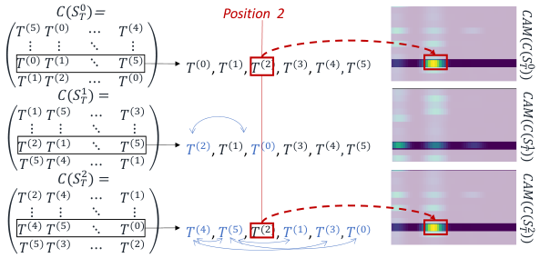
Figure 4 depicts an example of CAMs for different permutations. In this Figure, for three given permutations of (i.e., , and ), we notice that when is in position two of the second row of , the Class Activation Map is greater than when is not in position two. We infer that the second dimension of in position two is responsible for the high value. Thus, we may examine different dimension combinations by keeping track of which dimension at which position is activating the CAM the most. We now describe the steps necessary to retrieve this information.
Definition 0.
For a given data series of length and its input data structure , we define function , such that returns the row indices in that contain the dimension at position .
We can now define the following transformation .
Definition 0.
For a given data series of length , a given class and Class Activation Map, we define (with and its row) as follows:
| (3) |

Figure 5 depicts the transformation. As explained in Definition 2, the transformation enriches the Class Activation Map by adding the dimension position information. Note that if we change the dimension order of , their changes as well. Indeed, for a given dimension and position , will not have the same value for two different dimension orders of . Thus, computing for different dimension orders of will provide distinct information regarding the importance of a given position (subsequence) in a given dimension. We expect that subsequences (of a specific dimension) that discriminate one class from another will also be associated (most of the time) with a high value in the Class Activation Map.

4.4.2. Merging Permutations
We compute , for different .Note that the total number of permutations for high-dimensional data series is enormous: . In practice, we only compute for a randomly selected subset of . We thus merge permutations , by computing the averaged matrix of all the transformations of the permutations:
Figure 6 illustrates the process of computing from the set of permutations of , . can be seen as a summarization of the importance of each dimension at each position in , for all the computed permutations. Figure 6(b’) (at the top of the figure) depicts , which corresponds to the row (i.e., the dotted box in Figure 6(b)) of . Each row of corresponds to the average activation of dimension (for each timestamp) when dimension is in a given position in .
Note that all permutations of are forwarded into the dCNN network without training it again. Thus, even though the permutations of generate radically different inputs to the network, the network can still classify most of the instances correctly. For permutations, we use to denote the number of permutations that the model has correctly classified. We provide an analysis (see Section 5) of w.r.t the classification accuracy of the model and the impact that has on the discriminant features identification accuracy.
4.4.3. dCAM Extraction
We can now use the previously computed to extract explanatory information on which subsequences are considered important by the network. First, we note that each row of corresponds to the input format of the standard CNN architecture. Thus, we expect that the result of a row of (one of the ten lines in Figure 6(b)) is similar to the standard CAM. Hence, we can assume that is equivalent to standard Class Activation Map (this approximation is depicted in Figure 6(d)). Moreover, in addition to the temporal information, we can extract temporal information per dimension. We know that for a given position and a given dimension , represents the averaged activation for a given set of permutations. If the activation for a given dimension is constant (regardless of its value, or the position ), then the position of dimension is not important, and no subsequence in that dimension is discriminant. On the other hand, a high or low value at a specific position means that the subsequence at this specific position is discriminant. While it is intuitive to interpret a high value, interpreting a low value is counterintuitive. Usually, a subsequence at position with a low value should be regarded as non-discriminant. Nevertheless, if the activation is low for and high for other positions, then the subsequence at position is the consequence of the low value and is thus discriminant. We experimentally observe this situation, where a non-discriminant dimension has a constant activation per position (e.g., see dotted red rectangle in Figure 6(b): this pattern corresponds to a non-discriminant subsequence of the dataset). On the contrary, for discriminant dimensions, we observe a strong variance for the activation per position: either high values or low values (e.g., see solid red rectangles in Figure 6(b): these patterns correspond to the (injected) discriminant subsequences highlighted in red in Figure 6(e)). We thus can extract the significant subsequences per dimension by computing the variance of all positions of a given dimension. We can filter out the irrelevant temporal windows using the averaged for all dimensions, and use the variance to identify the important dimensions in the relevant temporal windows. Formally, we define as follows.
Definition 0.
For a data series and class , is:
| (4) |
4.5. Time Complexity Analysis
[Training step]: CNN/ResNet/InceptionTime require computations per kernel, while dCNN/dResNet/dInceptionTime require computations per kernel. Thus, the training time per epoch is higher for dCNN than CNN. However, given that the size of the input of dCNN is larger (containing permutations of a single series) than CNN, the number of epochs to reach convergence is lower for dCNN when compared to CNN. Intuitively, dCNN trains on more data during a single epoch. This leads to similar overall training times (see Section 5.7).
[dCAM step]: The CAM computation complexity is , where is the number of filters in the last convolutional layer. Let be the number of filters of the convolutional layers. Then, a forward pass has time complexity . In dCAM, we evaluate different permutations. Thus, the overall dCAM complexity is . Observe that since the permutations can be computed in parallel, the most important parameter for the execution time is .
4.6. Further Observations
We note that since in real use cases, labels are not available, the number of correctly classified permutations (called ) could be used as a proxy to assess the quality of the explanation (see Section 5.6).
Moreover, when analyzing sets of series, we can use dCAM on each one independently, and then aggregate the dCAM results to identify global discriminant features (see Section 5.8).
5. Experimental Evaluation
5.1. Experimental Setup
We implemented our algorithms in Python 3.5 using the PyTorch library (Paszke et al. 2019). The evaluation was conducted on a server with Intel Core i7-8750H CPU 2.20GHz x 12, with 31.3GB RAM, and Quadro P1000/PCle/SSE2 GPU with 4.2GB RAM, and on Jean Zay cluster with Nvidia Tesla V100 SXM2 GPU with 32 GB RAM.
Our code and datasets are available online (our 2022).
5.1.1. Datasets
We conduct our experimental evaluation using real datasets from the UCR/UEA archive (Dau et al. 2019) to evaluate the classification performance of the competing methods. The real datasets are injected with known discriminant patterns and a real use case from the medical domain to evaluate the discriminant features identification. We use the StarLightCurves (classes 2 and 3 only), ShapesAll (classes 1 and 2 only), and Fish (class 1 and 2 only) datasets from the UCR archive (Dau et al. 2019), in which we inject subsequences that will generate discriminant features. We build two types of datasets to study the ability of the algorithms to identify the discriminant patterns guiding the classification decision, (1) when these patterns occur in a subset of the dimensions at different timestamps, and (2) when these patterns occur in a subset of the dimensions at the same timestamp.
(1) For the datasets, we build each dimension of Class 1 by concatenating random instances from one class of one of our two UCR seed datasets. We build Class 2 by injecting in the series of the other class of our two UCR datasets a pattern in random dimensions at a random position in the series.
(2) For the datasets, we build each dimension of Class 1 by concatenating random instances from one of the classes of our two UCR datasets and injecting patterns from the other class in random dimensions and at different positions. We build Class 2 by injecting patterns at the same positions of random dimensions.
5.1.2. Evaluation Measures
We first evaluate the classification accuracy, -. This measure corresponds to the ratio of correctly classified instances among all instances in the test dataset.
We then evaluate the discriminant features accuracy, -, for Class 1 (see Figure 7). We define - as the PR-AUC for CAM/cCAM/dCAM obtained from the models and the ground-truth. The ground-truth is a series that has at the positions of discriminant features (see Figure 7(a.2): ground-truth contains at the positions of the injected patterns, marked with the red rectangles, and otherwise). We motivate the choice of PR-AUC (instead of ROC-AUC) because we are more interested in measuring the accuracy of identifying the injected patterns (representing at max 0.02 percent of the dataset) than measuring the accuracy of not detecting the non-injected patterns. In this very unbalanced case, PR-AUC is more appropriate than ROC AUC (Davis and Goadrich 2006).
Note that even though we annotate each point of the injected subsequences as discriminant, only some subparts of these sequences may be discriminant, thus, leading to - less than . Finally, for CNN/ResNet/InceptionTime, we compute the - scores by assuming that their (univariate) CAM values are the same for all dimensions. We mark their - scores with a star in Table 2.
5.2. Baselines and Training Setup
We compare our model, dCNN/dResNet/dInceptionTime, to the classical CNN/ResNet/InceptionTime model (Ismail Fawaz et al. 2018; Ismail Fawaz et al. 2019; Wang et al. 2017; Ismail Fawaz et al. 2020), and the cCNN/cResNet/cInceptionTime baseline we introduced in Section 2. We are using the same architecture setup for all models. We then use CAM for CNN, ResNet, InceptionTime, cCAM for cCNN, cResNet and cInceptionTime and dCAM for dCNN, dResNet and dInceptionTime to identify discriminant features. For CNN, cCNN and dCNN, we are using 5 convolutional layers with filters respectively. We are using a kernel size of 3 and a padding of 2. For ResNet, cResNet, and dResNet, we are using three blocks with three convolutional layers of 64 filters (for the first two blocks) and 128 layers (for the last block). We are using kernel sizes equal to 8, 5, and 3 for each block for the three layers of the block. For InceptionTime, cInceptionTime and dInceptionTime, we are using the same architecture as originally defined (Ismail Fawaz et al. 2020).
We also include MTEX-CNN (Assaf et al. 2019)(MTEX) as a baseline, representative of other kinds of architectures that can provide a multivariate CAM. The explanation is computed separately for discriminant features and timestamps using grad-CAM (Selvaraju et al. 2017) (MTEX-grad). The latter is a variant of the usual CAM using the gradients of the weights instead of the GAP layer to compute the activation.
We finally include three recurrent neural networks: the usual Recurrent Neural Network (Rumelhart et al. 1986) (RNN), Long-Short Term Memory (Hochreiter and Schmidhuber 1997) (LSTM), and Gated Recurrent Unit (Cho et al. 2014) (GRU) to our benchmark. As following previous evaluation work conducted in the UCR/UEA archive (Smirnov and Mephu Nguifo 2018), we use for all networks one recurrent hidden layer (RNN, LSTM, and GRU respectively) of 128 neurons. We then add one dense layer connecting the 128 neurons to the classes neurons.
We split our dataset into training and validation sets with 80 and 20 percent of the total dataset, respectively (equally balanced between the two classes). The training dataset is used to train the model, and the validation dataset is used as a validation dataset during the training phase. We generate a fully new test dataset for synthetic datasets and evaluate - and -. We train all models with a learning rate , a maximum batch size of 16 instances (less if GPU memory cannot fit 16 instances), and a maximal number of epochs equal to 1000 (we use early stopping and stop before 1000 epochs if the model starts overfitting the test dataset). For dCAM, we use (number of random permutations), a value that we empirically verified (due to lack of space, a detailed analysis of the effect of is in the full version of the paper).
5.3. Classification Accuracy evaluation
| Metadata | - (averaged on 10 runs) | |||||||||||||||
| Baselines | c-Baselines | d-Baselines | ||||||||||||||
| Datasets name | RNN | GRU | LSTM | MTEX | CNN | ResNet | InceptionT. | cCNN | cResNet | cInceptionT. | dCNN | dResNet | dInceptionT. | |||
| AtrialFibrillation | 3 | 640 | 2 | 0.66 | 0.70 | 0.66 | 0.72 | 0.41 | 0.40 | 0.64 | 0.56 | 0.53 | 0.68 | 0.49 | 0.45 | 0.61 |
| Libras | 15 | 45 | 2 | 0.86 | 0.84 | 0.75 | 0.93 | 0.96 | 0.96 | 0.82 | 0.80 | 0.82 | 0.65 | 0.91 | 0.94 | 0.66 |
| BasicMotions | 4 | 100 | 2 | 0.68 | 0.87 | 0.83 | 0.91 | 1.00 | 1.00 | 1.00 | 1.00 | 1.00 | 1.00 | 1.00 | 1.00 | 1.00 |
| RacketSports | 4 | 30 | 6 | 0.70 | 0.78 | 0.75 | 0.81 | 0.94 | 0.99 | 0.90 | 0.95 | 0.98 | 0.85 | 0.94 | 0.98 | 0.92 |
| Epilepsy | 4 | 206 | 3 | 0.63 | 0.83 | 0.83 | 0.97 | 1.00 | 1.00 | 0.97 | 1.00 | 1.00 | 1.00 | 1.00 | 1.00 | 0.99 |
| StandWalkJump | 3 | 2500 | 4 | 0.60 | 0.80 | 0.90 | 0.66 | 0.70 | 0.66 | 0.65 | 0.83 | 1.00 | 0.81 | 0.95 | 1.00 | 0.75 |
| UWaveGest.Lib. | 8 | 315 | 3 | 0.88 | 0.93 | 0.88 | 0.93 | 0.88 | 0.89 | 0.89 | 0.76 | 0.74 | 0.64 | 0.84 | 0.89 | 0.83 |
| Handwriting | 26 | 152 | 3 | 0.45 | 0.43 | 0.40 | 0.34 | 0.83 | 0.90 | 0.55 | 0.42 | 0.70 | 0.38 | 0.76 | 0.89 | 0.52 |
| NATOPS | 6 | 51 | 24 | 0.87 | 0.91 | 0.82 | 0.91 | 0.99 | 1.00 | 0.95 | 0.86 | 0.89 | 0.83 | 0.97 | 0.99 | 0.91 |
| PenDigits | 10 | 8 | 2 | 0.99 | 0.99 | 0.99 | 0.99 | 0.99 | 0.99 | 0.99 | 0.99 | 0.99 | 0.99 | 0.99 | 0.99 | 0.99 |
| FingerMovements | 2 | 50 | 28 | 0.56 | 0.58 | 0.58 | 0.62 | 0.70 | 0.68 | 0.71 | 0.57 | 0.63 | 0.55 | 0.72 | 0.71 | 0.66 |
| Artic.WordRec. | 25 | 144 | 9 | 0.98 | 0.97 | 0.90 | 0.98 | 0.99 | 0.99 | 0.93 | 0.82 | 0.94 | 0.74 | 0.98 | 0.99 | 0.88 |
| HandMov.Dir. | 4 | 400 | 10 | 0.46 | 0.40 | 0.37 | 0.44 | 0.44 | 0.42 | 0.51 | 0.34 | 0.35 | 0.40 | 0.45 | 0.44 | 0.33 |
| Cricket | 12 | 1197 | 6 | 0.98 | 0.90 | 0.80 | 0.95 | 1.00 | 1.00 | 0.98 | 0.94 | 0.97 | 0.87 | 1.00 | 1.00 | 0.98 |
| LSST | 14 | 36 | 6 | 0.54 | 0.53 | 0.52 | 0.53 | 0.62 | 0.66 | 0.40 | 0.56 | 0.59 | 0.49 | 0.62 | 0.66 | 0.51 |
| Eth.Concentration | 4 | 1751 | 3 | 0.33 | 0.37 | 0.32 | 0.58 | 0.35 | 0.36 | 0.34 | 0.36 | 0.36 | 0.36 | 0.35 | 0.39 | 0.34 |
| SelfReg.SCP1 | 2 | 896 | 6 | 0.91 | 0.88 | 0.89 | 0.88 | 0.86 | 0.83 | 0.87 | 0.88 | 0.84 | 0.88 | 0.86 | 0.86 | 0.88 |
| SelfReg.SCP2 | 2 | 1152 | 7 | 0.58 | 0.57 | 0.60 | 0.58 | 0.59 | 0.58 | 0.62 | 0.60 | 0.59 | 0.59 | 0.57 | 0.60 | 0.63 |
| Heartbeat | 2 | 405 | 61 | 0.73 | 0.73 | 0.73 | 0.75 | 0.83 | 0.86 | 0.83 | 0.76 | 0.76 | 0.76 | 0.84 | 0.86 | 0.83 |
| PhonemeSpectra | 39 | 217 | 39 | 0.11 | 0.11 | 0.11 | 0.15 | 0.31 | 0.37 | 0.27 | 0.31 | 0.33 | 0.28 | 0.33 | 0.40 | 0.32 |
| EigenWorms | 5 | 17984 | 6 | 0.57 | 0.50 | 0.66 | 0.57 | 0.90 | 0.92 | 0.82 | 0.71 | 0.92 | 0.73 | 0.92 | 0.92 | 0.81 |
| MotorImagery | 2 | 3000 | 64 | 0.53 | 0.59 | 0.58 | 0.59 | 0.58 | 0.57 | 0.56 | 0.56 | 0.57 | 0.56 | 0.65 | 0.68 | 0.66 |
| FaceDetection | 2 | 62 | 144 | 0.64 | 0.58 | 0.60 | 0.72 | 0.57 | 0.59 | 0.71 | 0.55 | 0.70 | 0.70 | 0.57 | 0.61 | 0.63 |
| Mean | 0.662 | 0.686 | 0.672 | 0.717 | 0.758 | 0.766 | 0.735 | 0.701 | 0.747 | 0.684 | 0.770 | 0.793 | 0.723 | |||
| Rank | 8.26 | 7.65 | 8.73 | 6.39 | 4.73 | 4.13 | 6.08 | 7.30 | 5.73 | 7.73 | 4.56 | 2.65 | 6.56 | |||
We first evaluate the classification performance of our proposed approaches (denoted as -Baselines and -Baselines in Table 2) and the different baselines (denoted as Baselines in Table 2) over the UCR/UEA multivariate data series. We run each method ten times and report the average -.
We first observe that the recurrent models (RNN, GRU, LSTM) are less accurate by approximately 0.10 than CNN-based models (CNN, ResNet and InceptionTime). These results confirm the observations of previous works (Ismail Fawaz et al. 2018; Ismail Fawaz et al. 2019; Wang et al. 2017; Ruiz et al. 2021). We then observe that ResNet-based architecture performs better than CNN-based and InceptionTime-based architectures. Moreover, we note that, overall, dCNN and dResNet have a better - than CNN and ResNet, respectively. This observation confirms that our proposed architectures (dResNet, dCNN) do not result in any loss in accuracy; on the contrary, they are slightly more accurate than usual architectures (ResNet, CNN). We notice that dResNet is, on average, one rank higher than ResNet. Similar observations can be made when comparing dCNN and CNN.
Moreover, Table 2 confirms that using cCNN baselines (or cResNet and cInceptionTime) implies a drop in classification accuracy. For instance, CNN architecture is 0.05 more accurate than cCNN architecture. Thus, -Baselines cannot guarantee at least equivalent accuracy. Figure 8(a) depicts the comparison between dCNN - (on the y-axis) and CNN/cCNN - (on the x-axis; CNN: blue circles; cCNN: red crosses). The dotted line corresponds to cases when both classifiers have the same accuracy. We observe that almost all cCNN - (red crosses) are above the dotted line, which shows that dCNN is more accurate for most datasets. Similarly, we observe that most of the CNN - (blue circles) are above the dotted lines, which means that dCNN is more accurate than CNN. The same observation can be made when examining Figure 8(b), in which dResNet is compared with ResNet and cResNet.
However, the same observation is not true when comparing dInceptionTime with InceptionTime and cInceptionTime. Even though in Figure 8(c) most of the red crosses are above the dotted line, indicating that dInceptionTime is most of the time more accurate than cInceptionTime, the blue circles are equally distributed above and under the dotted line. Thus, dInceptionTime is not more accurate than InceptionTime. The results in Table 2 also show that the averaged - across all datasets (as well as the averaged rank) is lower for dInceptionTime than for InceptionTime. Nevertheless, the performance of dInceptionTime is very close to that of InceptionTime. Thus, transforming the original architecture into one that supports dCAM does not penalize classification performance.
Finally, we observe that the accuracy of MTEX-CNN is lower than that of Baselines and the d-Baselines. We note that MTEX-CNN and cCNN have very similar performance (average accuracy of 0.71 and 0.70, and average rankings of 6.39 and 7.30). As we explained earlier (see Section 2.3), the MTEX-CNN architecture is divided into two blocks. The experiments demonstrate that the 2nd block cannot capture all discriminant features, and thus, cannot reach the accuracy of a traditional CNN. We conclude that MTEX-CNN is not as accurate as traditional architectures (such as CNN) or our proposed architectures (such as dCNN).
5.4. Discriminant Features Identification
| Datasets | - (averaged on 10 runs) | - (averaged on 50 instances) | |||||||||||||
| MTEX-grad | CAM | cCAM | dCAM | ||||||||||||
| Dataset name | Type | Dimensions | MTEX | ResNet | cResNet | dCNN | dResNet | dInception | MTEX | ResNet | cResNet | dCNN | dResNet | dInception | Random |
| StarLightCurve | Type 1 | 10 | 0.99 | 0.95 | 1.00 | 1.00 | 1.00 | 1.00 | 0.40 | 0.07* | 0.92 | 0.46 | 0.38 | 0.21 | 0.02 |
| 20 | 0.99 | 0.71 | 1.00 | 1.00 | 1.00 | 0.98 | 0.38 | 0.02* | 0.92 | 0.38 | 0.45 | 0.36 | 0.01 | ||
| 40 | 0.98 | 0.60 | 1.00 | 0.99 | 1.00 | 0.93 | 0.24 | 0.008* | 0.94 | 0.28 | 0.42 | 0.39 | 0.005 | ||
| 60 | 0.61 | 0.57 | 1.00 | 0.98 | 0.99 | 0.91 | 0.05 | 0.004* | 0.92 | 0.23 | 0.24 | 0.13 | 0.003 | ||
| 100 | 0.55 | 0.64 | 1.00 | 0.96 | 0.97 | 0.79 | 0.01 | 0.003* | 0.92 | 0.2 | 0.26 | 0.10 | 0.002 | ||
| Type 2 | 10 | 0.58 | 0.71 | 0.53 | 1.00 | 1.00 | 0.93 | 0.15 | 0.0256* | 0.025 | 0.26 | 0.43 | 0.10 | 0.021 | |
| 20 | 0.55 | 0.61 | 0.55 | 0.98 | 1.00 | 0.70 | 0.04 | 0.016* | 0.01 | 0.28 | 0.43 | 0.05 | 0.01 | ||
| 40 | 0.56 | 0.58 | 0.51 | 0.88 | 0.58 | 0.56 | 0.07 | 0.0068* | 0.006 | 0.20 | 0.05 | 0.03 | 0.005 | ||
| 60 | 0.53 | 0.55 | 0.53 | 0.64 | 0.59 | 0.55 | 0.008 | 0.0058* | 0.005 | 0.01 | 0.003 | 0.009 | 0.003 | ||
| 100 | 0.52 | 0.59 | 0.5 | 0.59 | 0.56 | 0.60 | 0.01 | 0.0024* | 0.002 | 0.003 | 0.004 | 0.02 | 0.002 | ||
| ShapesAll | Type 1 | 10 | 1.00 | 1.00 | 1.00 | 1.00 | 1.00 | 1.00 | 0.60 | 0.09* | 0.79 | 0.66 | 0.7 | 0.55 | 0.02 |
| 20 | 1.00 | 0.86 | 1.00 | 1.00 | 1.00 | 0.99 | 0.31 | 0.03* | 0.74 | 0.56 | 0.66 | 0.51 | 0.011 | ||
| 40 | 0.85 | 0.65 | 1.00 | 1.00 | 1.00 | 1.00 | 0.20 | 0.008* | 0.88 | 0.45 | 0.74 | 0.76 | 0.005 | ||
| 60 | 0.83 | 0.65 | 1.00 | 1.00 | 1.00 | 0.96 | 0.50 | 0.005* | 0.65 | 0.44 | 0.72 | 0.79 | 0.003 | ||
| 100 | 0.70 | 0.57 | 1.00 | 0.98 | 1.00 | 0.85 | 0.002 | 0.003* | 0.83 | 0.31 | 0.49 | 0.48 | 0.002 | ||
| Type 2 | 10 | 0.60 | 0.82 | 0.54 | 1.00 | 1.00 | 0.93 | 0.02 | 0.0467* | 0.04 | 0.63 | 0.50 | 0.32 | 0.02 | |
| 20 | 0.54 | 0.57 | 0.52 | 1.00 | 1.00 | 0.89 | 0.04 | 0.0132* | 0.013 | 0.50 | 0.73 | 0.40 | 0.01 | ||
| 40 | 0.59 | 0.60 | 0.52 | 0.90 | 0.72 | 0.73 | 0.02 | 0.005* | 0.005 | 0.40 | 0.20 | 0.36 | 0.005 | ||
| 60 | 0.57 | 0.59 | 0.51 | 0.65 | 0.61 | 0.72 | 0.06 | 0.0037* | 0.003 | 0.22 | 0.34 | 0.46 | 0.003 | ||
| 100 | 0.52 | 0.59 | 0.50 | 0.55 | 0.58 | 0.55 | 0.04 | 0.0027* | 0.002 | 0.005 | 0.02 | 0.05 | 0.002 | ||
| Rank | 3.95 | 3.9 | 3 | 1.65 | 1.6 | 2.85 | 3.85 | 4.45 | 3 | 2.6 | 2.15 | 2.75 | |||
We now evaluate the classification accuracy (-) and the discriminant features identification accuracy (-) on synthetically built datasets. Table 3 depicts both - and - on and datasets, when varying the number of dimensions from 10 to 100. In this experiment, we keep as baselines only ResNet and cResNet, which are the most accurate methods among all other baselines.
Overall, all methods have better performance (both - and -) on datasets than on . This was expected: discriminant features located in single dimensions are easier to find than discriminant features that depend on several dimensions.
We then notice that for low dimensional (=10) datasets, ResNet, dResNet, dCNN, and dInceptionTime are performing nearly perfect . Moreover, ResNet and MTEX-CNN are performing well for low-dimensional data series but start to fail for a more significant number of dimensions. While the drop is already significant for the dataset built from the StarLightCurve dataset, it is even stronger for datasets, for which ResNet fails to classify instances with a number of dimensions . On the contrary, dCNN, dResNet, and dInceptionTime, which use the random permutations in the input, are not sensitive to the number of dimensions and have an almost perfect - for most of datasets. We observe a - drop for dCNN, dResNet and dInceptionTime as dimensions increase for datasets. However, this drop is significantly less pronounced than that of ResNet. Overall, dCNN, dResNet, and dInceptionTime, which have on average the three highest ranks, are the most accurate methods.
Regarding cResNet, although it achieves a nearly perfect for datasets, we observe that it fails to classify correctly instances of datasets. As explained in Section 2, the input data structure is not rich enough to allow comparisons among dimensions, which is the main way to find discriminant features between the two classes of datasets. We also observe that MTEX-CNN fails to classify instances of datasets. Thus, this architecture does not correctly detect the discriminant features across different dimensions. Overall, Figure 9(a) shows that dCNN, dResNet and dInceptionTime are equivalent to cResNet for (Figure 9(a.1)), outperforming all the baselines for (Figure 9(a.2)), and in general are better than the baselines (ResNet and cResNet) for both types (Figure 9(a.3) with ).
We now compare the different methods using the - measure. We observe that the baseline cCAM (computed with cCNN) is outperforming CAM (computed with ResNet) and dCAM (with all of dCNN, dResNet and dInceptionTime) for datasets. This is explained by the fact that these classes can be discriminated by treating dimensions independently. Thus, cCAM (with no comparisons between dimensions) is naturally the best solution. Nevertheless, as datasets require comparisons among dimensions to discriminate the classes, cCAM fails on them, with a - very similar to the one of a random classifier. This confirms that such a baseline cannot be considered as a general solution for multivariate data series classification. We also observe that - of the explanation method of MTEX-CNN (MTEX-grad) is lower than dCAM for and close to - of cCAM for , meaning that it cannot identify discriminant features of datasets.
We then compare CAM and dCAM (used with dCNN/dResNet/ dInceptionTime). Figure 9(b) shows that dCAM significantly outperforms CAM, and that - reduces for all models as the number of dimensions increases. Nevertheless, - of dCAM remains relatively high for both (Figure 9(b.1)) and (Figure 9(b.2)) datasets (for less than 60 dimensions).
This result demonstrates the superiority of dCAM over state-of-the-art methods. Besides, the average ranks in Table 3indicate that dCAM computed from ResNet has the highest rank of .
5.5. Influence of
This section analyzes the influence of the number of permutations on the discriminative features identification accuracy (-). We compute the - for 20 different instances for which dCAM is computed using a value of between and . We randomly select the 20 instances from the 9 ShapesAll datasets, and . (We excluded the ShapesAll dataset with 100 dimensions, because no model trained on this dataset leads to reasonably accurate results: see Table 3.) Figure 10(a.1) for datasets and (a.2) for datasets depicts the evolution of - (on average for the 20 instances) as increases, for dCNN, dResNet and dInception Time. The results show that the model architecture influences convergence speed, and that convergence speed reduces as the number of dimensions increases. Figure 10(b) shows that the number of permutations needed to reach 90 percents of the best - is greater when is higher. The latter holds for (Figure 10(b.1)) and datasets (Figure 10(b.2)). Overall, we notice that the dCAM computation with dResNet and dInceptionTime converges faster than dCNN. Studying deep neural network architectures that could reduce the number of permutations needed to reach the maximum - is an open research problem.

5.6. - versus -
In this section, we first analyze the relation between - and -. We then evaluate the impact that - has on the number of permutations that have been correctly classified . We finally evaluate the impact that has on -.
Figure 11(1) depicts the relation between - and - for dCNN (Figure 11(a.1)), dResNet (Figure 11(b.1)) and dInceptionTime (Figure 11(c.1)) for all synthetic datasets. Note that all methods have a logarithmic relation (dotted red line) between - (x-axis) and - (y-axis). This confirms that the accuracy of the trained model has a significant impact on discriminant feature identification.
Figure 11(3) depicts on the y-axis the ratio of correctly classified permutations () among all permutations () versus the - (on the x-axis). In this case, for all of dCNN (Figure 11(a.3)), dResNet (Figure 11(b.3)) and dInceptionTime (Figure 11(c.3)), we observe that there exists a linear relationship for - between 0.7 and 1. This means that will be greater when the model is more accurate. Nevertheless, for - between 0.5 and 0.7, we observe a high variance for . Thus, an inaccurate model may still lead to a high . Finally, Figure 11(2) depicts the relation between (on the y-axis) and - (on the x-axis). We observe a similar relationship between - and -, which means that a low may lead to inaccurate discriminant features identification.
As hypothesized in Section 4, the experimental results confirm that an inaccurate model (for all of dCNN, dResNet, and dInceptionTime) cannot be used to identify discriminant features. Moreover, since in a real use-case it is not possible to measure -, we can use to estimate the discriminant feature identification accuracy. Even though Figure 11(2) demonstrates that a high does not always lead to a high -, in practice, we can safely assume that a low will most probably correspond to a low -. Therefore, such measure can be used as a proxy for the estimation of the explanation quality.
5.7. Execution time evaluation
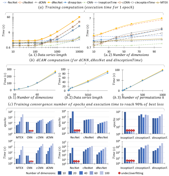

In this section, we evaluate the execution time of our proposed approaches and the baselines. Figure 12(a) depicts the training execution time (for one epoch) when we vary the data series length with a constant number of dimensions fixed to 10 (Figure 12(a.1)), and when we vary the number of dimensions with a constant data series length fixed to 100 (Figure 12(a.2)). In these two experiments, we use a batch size of 4 for all models. Overall, CNN and InceptionTime-based architectures are faster than ResNet-based architectures, and CNN, ResNet, InceptionTime, and MTEX-CNN are faster when the number of dimensions and the data series length is increasing. Nevertheless, both dCNN/dResNet/dInceptionTime and cCNN/cResNet/cInceptionTime require the same training time.
We now evaluate the execution time and the number of epochs required to train our proposed approaches and the baselines. Figure 12(c) depicts the time (in seconds) and the number of epochs to reach 90% of the best loss (on the test set) for ShapesAll datasets varying the number of dimensions between 10 and 100. We use for all models a batch size of 16. The red dot indicates that a model is either overfitted or underfitted (i.e., the loss for the first epoch is approximately equal to the best loss). We observe that cCNN/cResNet/cInceptionTime and dCNN/dResNet/dInceptionTime require the same amount of time to be trained, but traditional baselines require more epochs than the proposed d-methods. Thus, training time for ResNet is longer than dResNet for and .
Finally, we measure the execution time required to compute dCAM (for dCNN, dResNet, and dInceptionTime), when we vary the number of dimensions with a constant data series length fixed to 400 (Figure 12(b.1)), when we vary the data series length with a constant number of dimensions fixed to 10 (Figure 12(b.2)), and when we vary the number of permutations (Figure 12(b.3)). Note that the dCAM execution times are very similar for the three types of architectures. Moreover, the execution time increases super-linearly with the number of dimensions but is linear to the data series length and the number of permutations .
5.8. Use Case: Surgeon skills explanation
We now illustrate the applicability of our method to a real-world use case. In this use case, we train our dCNN network on the JIGSAWS dataset (Gao et al. 2014) to identify novice surgeons, based on kinematic data series when performing surgical suturing tasks (i.e., wound stitching) using robotic arms and surgical grippers.
[Dataset] The data series are recorded from the . The multivariate data series are composed of dimensions (an example of multivariate data series is depicted in Figure 13(a)). Each dimension corresponds to a sensor (with an acquisition rate of Hz). The sensors are divided into four groups: patient-side manipulators (left and right PSMs: green rectangle in Figure 13(a) top left), and left and right master tool manipulators (left and right MTMs: blue rectangle in Figure 13(a) bottom left). Each group contains 19 sensors. These sensors are: 3 variables for the Cartesian position of the manipulator, 9 variables for the rotation matrix, 6 variables for the linear and angular velocity of the manipulator, and 1 variable for the gripper angle.
To perform a suture, the surgeons perform different gestures (11 in total). For example, refers to reaching for the needle with the right hand, while refers to dropping the suture at the end and moving to end points. Each gesture corresponds to a specific time segment of the dataset, involving all sensors. For example, the dotted red rectangle in Figure 13(a) represents gesture : pulling the suture with the left hand. Surgeons that reported having more than 100 hours of experience are considered experts, surgeons with 10-100 hours are considered intermediate, and surgeons with less than 10 hours are labeled as novices. We have 19 multivariate data series in the novice class, denoted as , 10 in the intermediate, , 10 multivariate data series in the expert class, . More information on this dataset can be found in (Gao et al. 2014).
[Training] For the training procedure, we use 80% of the dataset (randomly selected from the three classes) for training. The rest 20% of the dataset is used for validation and early stopping. Since the instances do not have the same length, we use batches composed of one instance when training the models in the GPU.
[Evaluation] Similar to what has been reported in previous work (Ismail Fawaz et al. 2018), we achieve 100% accuracy on the train and test datasets (for ten different randomly selected train and test sets). We proceed to compute the for every instance of the novice class . The of the multivariate data series named _ (Figure 13(a)) is displayed in Figure 13(b). In the latter, the deep blue color indicates low activated subsequences (i.e., non-discriminant of belonging to the novice class ), while the yellow color is pointing to highly activated subsequences. First, we note that some groups of sensors (dimensions) are more activated than others. In Figure 13(b), the left and right "MTM gripper angles" are the most activated sensors. Figure 13(c), which depicts the box-plot of the maximal activated values per sensor, confirms that in the general case, MTM gripper angles, as well as the MTM and PSM tooltip rotation matrices (three of these sensors are highlighted in red in Figure 13(a)), are the most discriminant sensors. On the contrary, linear and angular speeds are not discriminant and hence cannot explain the novice class .
As explained in Section 4.6, we now extract global explanations at the scale of the dataset. We compute the dCAM for each instance, and we then extract global statistics on the sensors, i.e., aggregated over all instances. Figure 13(d) depicts the averaged activation per sensor per gesture. Overall, identifies gesture (using the right hand to help tighten the suture) as a discriminant gesture, because of the discriminant subsequences present in the sensors "right MTM gripper angle", " element", and " element" (marked with red ovals in Figure 13(d)). These three identified sensors (dimensions) are relevant to the right PSM tooltip rotation matrix and are important for the suturing process. Similarly, we observe that gesture (i.e., pulling suture with left hand) is discriminant, and activated the most by the "left NTM gripper angle" sensor. This result is consistent with a previous study (Ismail Fawaz et al. 2018), which also identified gesture as discriminant of belonging to the novice class. Nevertheless, this previous study was using CAM to only highlight the time interval corresponding to gesture . On the contrary, dCAM provides more accurate (and useful) information: it does not only identify the discriminant gesture , but also the discriminant sensors. This allows the analysts to recognize exactly what aspects of the particular gesture are problematic.
[Summary] The application of dCAM in the robot-assisted surgeon training use case demonstrated its effectiveness. Our approach was able to provide meaningful explanations for the classification decisions, based on specific gestures (subsequences), and specific sensors (dimensions) that describe particular aspects of these gestures, i.e., the positioning and rotation angles of the tip of the stitch gripper. Such explanations can help surgeons to improve their skills.
6. Conclusions
Even though data series classification using deep learning has attracted a lot of attention, existing techniques for explaining the classification decisions fail for the case of multivariate data series. We described a novel approach, dCAM, based on CNNs, which detects discriminant subsequences within individual dimensions of a multivariate data series. The experimental evaluation with synthetic and real datasets demonstrates the superiority of our approach.
Acknowledgments Work supported by EDF R&D and ANRT French program, and HPC resources from GENCI-IDRIS (Grants 2020-101471 and 2021-101925), and NVIDIA Corporation for the Titan Xp GPU donation used in this research.
References
- (1)
- our (2022) 2022. dCAM Webpage. https://helios2.mi.parisdescartes.fr/˜themisp/dCAM/
- Assaf et al. (2019) Roy Assaf, Ioana Giurgiu, Frank Bagehorn, and Anika Schumann. 2019. MTEX-CNN: Multivariate Time Series EXplanations for Predictions with Convolutional Neural Networks. In 2019 IEEE International Conference on Data Mining (ICDM). 952–957. https://doi.org/10.1109/ICDM.2019.00106
- Bagnall et al. (2016) Anthony Bagnall, Jason Lines, Aaron Bostrom, James Large, and Eamonn Keogh. 2016. The great time series classification bake off: a review and experimental evaluation of recent algorithmic advances. Data Min. Knowl. Discov. 31 (2016).
- Bagnall et al. (2015) Anthony Bagnall, Jason Lines, Jon Hills, and Aaron Bostrom. 2015. Time-Series Classification with COTE: The Collective of Transformation-Based Ensembles. IEEE TKDE 27 (2015).
- Bagnall et al. (2019) Anthony J. Bagnall, Richard L. Cole, Themis Palpanas, and Konstantinos Zoumpatianos. 2019. Data Series Management (Dagstuhl Seminar 19282). Dagstuhl Reports 9, 7 (2019), 24–39.
- Boniol et al. (2021a) Paul Boniol, Michele Linardi, Federico Roncallo, Themis Palpanas, Mohammed Meftah, and Emmanuel Remy. 2021a. Unsupervised and Scalable Subsequence Anomaly Detectionin Large Data Series. VLDBJ (2021).
- Boniol and Palpanas (2020) Paul Boniol and Themis Palpanas. 2020. Series2Graph: Graph-based Subsequence Anomaly Detection for Time Series. Proc. VLDB Endow. 13, 11 (2020), 1821–1834.
- Boniol et al. (2021b) Paul Boniol, John Paparrizos, Themis Palpanas, and Michael J. Franklin. 2021b. SAND: Streaming Subsequence Anomaly Detection. Proc. VLDB Endow. 14, 10 (2021), 1717–1729.
- Chen et al. (2013) Huanhuan Chen, Fengzhen Tang, Peter Tino, and Xin Yao. 2013. Model-Based Kernel for Efficient Time Series Analysis. In ACM SIGKDD.
- Cho et al. (2014) Kyunghyun Cho, Bart van Merrienboer, Çaglar Gülçehre, Dzmitry Bahdanau, Fethi Bougares, Holger Schwenk, and Yoshua Bengio. 2014. Learning Phrase Representations using RNN Encoder-Decoder for Statistical Machine Translation. In Proceedings of the 2014 Conference on Empirical Methods in Natural Language Processing, EMNLP. ACL, 1724–1734.
- Cui et al. (2016) Zhicheng Cui, Wenlin Chen, and Yixin Chen. 2016. Multi-Scale Convolutional Neural Networks for Time Series Classification. CoRR (2016).
- Dau et al. (2019) H. A. Dau, A. Bagnall, K. Kamgar, C. M. Yeh, Y. Zhu, S. Gharghabi, C. A. Ratanamahatana, and E. Keogh. 2019. The UCR time series archive. IEEE/CAA J. Automatic. 6, 6 (2019).
- Davis and Goadrich (2006) Jesse Davis and Mark Goadrich. 2006. The Relationship between Precision-Recall and ROC Curves. In Proceedings of the 23rd International Conference on Machine Learning (Pittsburgh, Pennsylvania, USA) (ICML ’06). Association for Computing Machinery, New York, NY, USA, 233–240. https://doi.org/10.1145/1143844.1143874
- Dempster et al. (2020) Angus Dempster, François Petitjean, and Geoffrey I. Webb. 2020. ROCKET: exceptionally fast and accurate time series classification using random convolutional kernels. Data Min. Knowl. Discov. 34, 5 (2020), 1454–1495.
- Echihabi et al. (2022) Karima Echihabi, Panagiota Fatourou, Kostas Zoumbatianos, Themis Palpanas, and Houda Benbrahim. 2022. Hercules Against Data Series Similarity Search. PVLDB (2022).
- Echihabi et al. (2018) Karima Echihabi, Kostas Zoumpatianos, Themis Palpanas, and Houda Benbrahim. 2018. The Lernaean Hydra of Data Series Similarity Search: An Experimental Evaluation of the State of the Art. Proc. VLDB Endow. 12, 2 (2018), 112–127.
- Echihabi et al. (2019) Karima Echihabi, Kostas Zoumpatianos, Themis Palpanas, and Houda Benbrahim. 2019. Return of the Lernaean Hydra: Experimental Evaluation of Data Series Approximate Similarity Search. Proc. VLDB Endow. 13, 3 (2019), 403–420.
- Esling and Agon (2012) Philippe Esling and Carlos Agon. 2012. Time-series data mining. CSUR (2012).
- Gao and Lin (2019) Yifeng Gao and Jessica Lin. 2019. HIME: discovering variable-length motifs in large-scale time series. Knowl. Inf. Syst. 61, 1 (2019), 513–542.
- Gao et al. (2020) Yifeng Gao, Jessica Lin, and Constantin Brif. 2020. Ensemble Grammar Induction For Detecting Anomalies in Time Series. In Proceedings of the 23rd International Conference on Extending Database Technology, EDBT 2020, Copenhagen, Denmark, March 30 - April 02, 2020. OpenProceedings.org, 85–96.
- Gao et al. (2014) Yixin Gao, S. Vedula, Carol E. Reiley, N. Ahmidi, B. Varadarajan, Henry C. Lin, L. Tao, L. Zappella, B. Béjar, D. Yuh, C. C. Chen, R. Vidal, S. Khudanpur, and Gregory Hager. 2014. JHU-ISI Gesture and Skill Assessment Working Set ( JIGSAWS ) : A Surgical Activity Dataset for Human Motion Modeling.
- Gogolou et al. (2020) Anna Gogolou, Theophanis Tsandilas, Karima Echihabi, Anastasia Bezerianos, and Themis Palpanas. 2020. Data Series Progressive Similarity Search with Probabilistic Quality Guarantees. In Proceedings of the 2020 International Conference on Management of Data, SIGMOD Conference 2020, online conference [Portland, OR, USA], June 14-19, 2020. ACM, 1857–1873.
- Hochreiter and Schmidhuber (1997) Sepp Hochreiter and Jürgen Schmidhuber. 1997. Long Short-Term Memory. Neural Computation 9, 8 (1997), 1735–1780.
- Hsieh et al. (2021) Tsung-Yu Hsieh, Suhang Wang, Yiwei Sun, and Vasant Honavar. 2021. Explainable Multivariate Time Series Classification: A Deep Neural Network Which Learns to Attend to Important Variables As Well As Time Intervals. In Proceedings of the 14th ACM International Conference on Web Search and Data Mining (Virtual Event, Israel) (WSDM ’21). Association for Computing Machinery, New York, NY, USA, 607–615. https://doi.org/10.1145/3437963.3441815
- Ismail et al. (2020) Aya Abdelsalam Ismail, Mohamed K. Gunady, Héctor Corrada Bravo, and Soheil Feizi. 2020. Benchmarking Deep Learning Interpretability in Time Series Predictions. In Advances in Neural Information Processing Systems 33: Annual Conference on Neural Information Processing Systems 2020, NeurIPS 2020, December 6-12, 2020, virtual, Hugo Larochelle, Marc’Aurelio Ranzato, Raia Hadsell, Maria-Florina Balcan, and Hsuan-Tien Lin (Eds.). https://proceedings.neurips.cc/paper/2020/hash/47a3893cc405396a5c30d91320572d6d-Abstract.html
- Ismail Fawaz et al. (2018) Hassan Ismail Fawaz, Germain Forestier, Jonathan Weber, Lhassane Idoumghar, and Pierre-Alain Muller. 2018. Evaluating Surgical Skills from Kinematic Data Using Convolutional Neural Networks. In MICCAI.
- Ismail Fawaz et al. (2019) Hassan Ismail Fawaz, Germain Forestier, Jonathan Weber, Lhassane Idoumghar, and Pierre-Alain Muller. 2019. Deep Learning for Time Series Classification: A Review. Data Min. Knowl. Discov. 33, 4 (2019).
- Ismail Fawaz et al. (2020) Hassan Ismail Fawaz, Benjamin Lucas, Germain Forestier, Charlotte Pelletier, Daniel F. Schmidt, Jonathan Weber, Geoffrey I. Webb, Lhassane Idoumghar, Pierre Alain Muller, and François Petitjean. 2020. InceptionTime: finding AlexNet for time series classification. Data Mining and Knowledge Discovery 34 (7 Sept. 2020), 1936–1962.
- Jakovljevic et al. (2022) Luka Jakovljevic, Dimitre Kostadinov, Armen Aghasaryan, and Themis Palpanas. 2022. Towards Building a Digital Twin of Complex System Using Causal Modelling. In Complex Networks & Their Applications X. Springer International Publishing, Cham, 475–486.
- Kingma and Ba (2015) Diederik P. Kingma and Jimmy Ba. 2015. Adam: A Method for Stochastic Optimization. In ICLR.
- Krizhevsky et al. (2012) A. Krizhevsky, Ilya Sutskever, and Geoffrey E. Hinton. 2012. ImageNet classification with deep convolutional neural networks. Commun. ACM 60 (2012).
- Le Guennec et al. (2016) Arthur Le Guennec, Simon Malinowski, and Romain Tavenard. 2016. Data Augmentation for Time Series Classification using Convolutional Neural Networks. In ECML/PKDD on AALTD Workshop.
- LeCun et al. (2015) Yann LeCun, Yoshua Bengio, and Geoffrey Hinton. 2015. Deep learning. Nature 521 (2015).
- Levchenko et al. (2021) Oleksandra Levchenko, Boyan Kolev, Djamel Edine Yagoubi, Reza Akbarinia, Florent Masseglia, Themis Palpanas, Dennis E. Shasha, and Patrick Valduriez. 2021. BestNeighbor: efficient evaluation of kNN queries on large time series databases. Knowl. Inf. Syst. 63, 2 (2021), 349–378.
- Li et al. (2019) Xiaosheng Li, Jessica Lin, and Liang Zhao. 2019. Linear Time Complexity Time Series Clustering with Symbolic Pattern Forest. In Proceedings of the Twenty-Eighth International Joint Conference on Artificial Intelligence, IJCAI 2019, Macao, China, August 10-16, 2019, Sarit Kraus (Ed.). ijcai.org, 2930–2936.
- Linardi et al. (2020) Michele Linardi, Yan Zhu, Themis Palpanas, and Eamonn J. Keogh. 2020. Matrix profile goes MAD: variable-length motif and discord discovery in data series. Data Min. Knowl. Discov. 34, 4 (2020), 1022–1071.
- Lines et al. (2016) J. Lines, S. Taylor, and A. Bagnall. 2016. HIVE-COTE: The Hierarchical Vote Collective of Transformation-Based Ensembles for Time Series Classification. In IEEE ICDM.
- Lucas et al. (2019) Benjamin Lucas, Ahmed Shifaz, Charlotte Pelletier, Lachlan O’Neill, Nayyar A. Zaidi, Bart Goethals, François Petitjean, and Geoffrey I. Webb. 2019. Proximity Forest: an effective and scalable distance-based classifier for time series. Data Min. Knowl. Discov. 33, 3 (2019), 607–635.
- Nair and Hinton (2010) Vinod Nair and Geoffrey E. Hinton. 2010. Rectified Linear Units Improve Restricted Boltzmann Machines. In ICML.
- Palpanas (2015) Themis Palpanas. 2015. Data Series Management: The Road to Big Sequence Analytics. SIGMOD Rec. 44, 2 (2015), 47–52.
- Palpanas (2016) Themis Palpanas. 2016. Big Sequence Management: A glimpse of the Past, the Present, and the Future. In SOFSEM (Lecture Notes in Computer Science), Rusins Martins Freivalds, Gregor Engels, and Barbara Catania (Eds.), Vol. 9587. Springer, 63–80.
- Palpanas (2019) Themis Palpanas. 2019. Evolution of a Data Series Index. In ISIP.
- Palpanas and Beckmann (2019) Themis Palpanas and Volker Beckmann. 2019. Report on the First and Second Interdisciplinary Time Series Analysis Workshop (ITISA). SIGMOD Rec. 48, 3 (2019), 36–40.
- Paparrizos and Franklin (2019) John Paparrizos and Michael J. Franklin. 2019. GRAIL: Efficient Time-Series Representation Learning. Proc. VLDB Endow. 12, 11 (2019), 1762–1777.
- Paparrizos and Gravano (2016) John Paparrizos and Luis Gravano. 2016. k-Shape: Efficient and Accurate Clustering of Time Series. SIGMOD Rec. 45, 1 (2016), 69–76.
- Paparrizos and Gravano (2017) John Paparrizos and Luis Gravano. 2017. Fast and Accurate Time-Series Clustering. ACM Trans. Database Syst. 42, 2 (2017), 8:1–8:49.
- Paparrizos et al. (2022) John Paparrizos, Yuhao Kang, Paul Boniol, Ruey S. Tsay, Themis Palpanas, and Michael J. Franklin. 2022. TSB-UAD: An End-to-End Benchmark Suite for Univariate Time-Series Anomaly Detection. PVLDB (2022).
- Paszke et al. (2019) Adam Paszke, Sam Gross, Francisco Massa, Adam Lerer, James Bradbury, Gregory Chanan, Trevor Killeen, Zeming Lin, Natalia Gimelshein, Luca Antiga, Alban Desmaison, Andreas Kopf, Edward Yang, Zachary DeVito, Martin Raison, Alykhan Tejani, Sasank Chilamkurthy, Benoit Steiner, Lu Fang, Junjie Bai, and Soumith Chintala. 2019. PyTorch: An Imperative Style, High-Performance Deep Learning Library. In NeurIPS, Vol. 32.
- Peng et al. (2021a) Botao Peng, Panagiota Fatourou, and Themis Palpanas. 2021a. Fast Data Series Indexing for In-Memory Data. VLDBJ (2021).
- Peng et al. (2021b) Botao Peng, Panagiota Fatourou, and Themis Palpanas. 2021b. ParIS+: Data Series Indexing on Multi-Core Architectures. IEEE Trans. Knowl. Data Eng. 33, 5 (2021), 2151–2164.
- Peng et al. (2021c) Botao Peng, Panagiota Fatourou, and Themis Palpanas. 2021c. SING: Sequence Indexing Using GPUs. In ICDE.
- Ruiz et al. (2021) Alejandro Pasos Ruiz, Michael Flynn, James Large, Matthew Middlehurst, and Anthony J. Bagnall. 2021. The great multivariate time series classification bake off: a review and experimental evaluation of recent algorithmic advances. Data Min. Knowl. Discov. 35, 2 (2021), 401–449. https://doi.org/10.1007/s10618-020-00727-3
- Rumelhart et al. (1986) David E. Rumelhart, Geoffrey E. Hinton, and Ronald J. Williams. 1986. Learning representations by back-propagating errors. Nature 323 (1986), 533–536.
- Schäfer and Leser (2017) Patrick Schäfer and Ulf Leser. 2017. Fast and Accurate Time Series Classification with WEASEL. In Proceedings of the 2017 ACM on Conference on Information and Knowledge Management, CIKM 2017, Singapore, November 06 - 10, 2017. ACM, 637–646.
- Schäfer and Leser (2020) Patrick Schäfer and Ulf Leser. 2020. TEASER: early and accurate time series classification. Data Min. Knowl. Discov. 34, 5 (2020), 1336–1362.
- Schneider et al. (2021) J. Schneider, P. Wenig, and T. Papenbrock. 2021. Distributed detection of sequential anomalies in univariate time series. VLDBJ 30 (2021).
- Selvaraju et al. (2017) Ramprasaath R. Selvaraju, Michael Cogswell, Abhishek Das, Ramakrishna Vedantam, Devi Parikh, and Dhruv Batra. 2017. Grad-CAM: Visual Explanations from Deep Networks via Gradient-Based Localization. In 2017 IEEE International Conference on Computer Vision (ICCV). 618–626. https://doi.org/10.1109/ICCV.2017.74
- Serrà et al. (2018) J. Serrà, S. Pascual, and Alexandros Karatzoglou. 2018. Towards a universal neural network encoder for time series. In CCIA.
- Shifaz et al. (2020) Ahmed Shifaz, Charlotte Pelletier, François Petitjean, and Geoffrey I. Webb. 2020. TS-CHIEF: a scalable and accurate forest algorithm for time series classification. Data Min. Knowl. Discov. 34, 3 (2020), 742–775.
- Smirnov and Mephu Nguifo (2018) Denis Smirnov and Engelbert Mephu Nguifo. 2018. Time Series Classification with Recurrent Neural Networks. In ECML/PKDD Workshop on Advanced Analytics and Learning on Temporal Data (aaltd18).
- Tan et al. (2020) Chang Wei Tan, François Petitjean, and Geoffrey I. Webb. 2020. FastEE: Fast Ensembles of Elastic Distances for time series classification. Data Min. Knowl. Discov. 34, 1 (2020), 231–272.
- Ulanova et al. (2015) Liudmila Ulanova, Nurjahan Begum, and Eamonn J. Keogh. 2015. Scalable Clustering of Time Series with U-Shapelets. In Proceedings of the 2015 SIAM International Conference on Data Mining, Vancouver, BC, Canada, April 30 - May 2, 2015, Suresh Venkatasubramanian and Jieping Ye (Eds.). SIAM, 900–908.
- Wang et al. (2018) J. Wang, Z. Wang, Jianfeng Li, and J. Wu. 2018. Multilevel Wavelet Decomposition Network for Interpretable Time Series Analysis. ACM SIGKDD (2018).
- Wang and Palpanas (2021) Qitong Wang and Themis Palpanas. 2021. Deep Learning Embeddings for Data Series Similarity Search. In SIGKDD.
- Wang et al. (2017) Z. Wang, W. Yan, and T. Oates. 2017. Time series classification from scratch with deep neural networks: A strong baseline. In IJCNN.
- Xu et al. (2015) B. Xu, Naiyan Wang, T. Chen, and Mu Li. 2015. Empirical Evaluation of Rectified Activations in Convolutional Network. Deep Learning Workshop, ICML (2015).
- Yang and Wu (2006) Qiang Yang and Xindong Wu. 2006. 10 Challenging Problems in Data Mining Research. IJITDM 05, 04 (2006).
- Yankov et al. (2008) Dragomir Yankov, Eamonn J. Keogh, and Umaa Rebbapragada. 2008. Disk aware discord discovery: finding unusual time series in terabyte sized datasets. Knowl. Inf. Syst. 17, 2 (2008), 241–262.
- Ye and Keogh (2011) Lexiang Ye and Eamonn J. Keogh. 2011. Time series shapelets: a novel technique that allows accurate, interpretable and fast classification. Data Min. Knowl. Discov. 22, 1-2 (2011), 149–182.
- Zhang et al. (2019) Chuxu Zhang, Dongjin Song, Yuncong Chen, Xinyang Feng, Cristian Lumezanu, Wei Cheng, Jingchao Ni, Bo Zong, Haifeng Chen, and Nitesh V. Chawla. 2019. A Deep Neural Network for Unsupervised Anomaly Detection and Diagnosis in Multivariate Time Series Data. AAAI 33, 01 (2019).
- Zhang et al. (2020) Xuchao Zhang, Yifeng Gao, Jessica Lin, and Chang-Tien Lu. 2020. TapNet: Multivariate Time Series Classification with Attentional Prototypical Network. Proceedings of the AAAI Conference on Artificial Intelligence 34, 04 (Apr. 2020), 6845–6852. https://doi.org/10.1609/aaai.v34i04.6165
- Zhao et al. (2017) B. Zhao, H. Lu, S. Chen, J. Liu, and D. Wu. 2017. Convolutional neural networks for time series classification. J. Syst. Eng. Electron. 28, 1 (2017).
- Zheng et al. (2014) Yudi Zheng, Qi Liu, Enhong Chen, Yong Ge, and J. Leon Zhao. 2014. Time Series Classification Using Multi-Channels Deep Convolutional Neural Networks. In WAIM.
- Zhou et al. (2016) B. Zhou, A. Khosla, Lapedriza. A., A. Oliva, and A. Torralba. 2016. Learning Deep Features for Discriminative Localization. CVPR (2016).
- Zhu et al. (2021) Yan Zhu, Abdullah Mueen, and Eamonn J. Keogh. 2021. Matrix Profile IX: Admissible Time Series Motif Discovery With Missing Data. IEEE Trans. Knowl. Data Eng. 33, 6 (2021), 2616–2626.