Collaboration in Participant-Centric Federated Learning: A Game-Theoretical Perspective

In a global iteration, a participant’s model training cost consists of computation and communication cost.

Computation cost: The set of $K$ participants is denoted as $\mathcal{K}=\left\{1,2,...K\right\}$. Each participant $k$ owns a local dataset $\mathcal{D}_{k}=\{(\bm{x}_{k}^{1},y_{k}^{1}),...,(\bm{x}_{k}^{N_{k}},y_{k}^{N_{k}})\}$, and $|\mathcal{D}_{k}|$ denotes the data size of participant $k$, and $\bm{x}^{i}_{k}$ and $y_{k}^{i}$ represent the model features and the Ground truth label of participant $k$’s $i$-th data respectively. Similar to most existing approaches such as [18], we adopt the mini-batch stochastic gradient descent (SGD) algorithm for local training. Each participant selects a subset of the local dataset, called one batch, to calculate local gradients in one global iteration. The number of data samples in one batch selected by participant $k$ is $B_{k}$ and the global batchsize is $B=\sum_{k\in\mathcal{K}}B_{k}$. Obviously, $0\leq B_{k}\leq B_{k}^{max}\overset{\Delta}{=}|\mathcal{D}_{k}|$. To model a participant’s energy consumption, we further define $C_{k}$ as the average number of CPU cycles for participant $k$ performing local gradient calculation with one data sample. Moreover, $f_{k}$ is the adopted CPU processing speed (i.e., computing resource) of participant $k$ for local model training. In general, we have $f_{k}^{min}\leq f_{k}\leq f_{k}^{max}$ where $f_{k}^{min}$ and $f_{k}^{max}$ represent participant $k$’s minimum and maximum computing capabilities, respectively. Based on the above definitions, the energy consumption of local gradients calculation of participant $k$ in one global iteration can be calculated as [19]:

where $\alpha$ is a coefficent corresponding to the computing chip architecture. Also, the local training process latency can be calculated as:

Communication cost: At the phase of data communication, the local gradients are sent to the center server through the multiple channel access technology (e.g., orthogonal frequency division medium access (OFDMA)) once the local model training accomplished. The communication resource allocation optimization is usually determined by the central server instead of participants. Since we focus on analyzing the participants’ behaviors in participant-centric FL, we assume that the communication resource allocation for the participants’ data transmission is fixed. We also assume that the data size of the model parameter gradients is the same for each participant in each FL iteration (which is usually the case since all the participants train the same FL model). Thus, in this study we hence assume the communication cost is fixed for each participant in the following discussions ¹¹ 1 The communication cost for each participant can be different and this case can be captured by adding a participant-specific constant $D_{k}$ into the participant’s utility function in (6). Nevertheless, since the communication cost $D_{k}$ is fixed and does not impact participant’s decision on the computation resource allocation and batch size selection, we will neglect the fixed communication cost in the following analysis for simplicity. This simplicity is common in many exiting studies related to incentive mechanism design [20] [21] [22] and conducive to directly revealing economic characteristic for mechanism design, since the communication part is independent of FL model performance. .

We next turn attention to the participants’ utilities in participant-centric FL. In general, all participants aim to obtain a well-trained model with a low loss function (or high model accuracy). In one global iteration, higher model accuracy requires a larger global batchsize, which will further induce a higher training cost (i.e., local energy consumption and latency). In this regard, according to [18], we first define the global loss function and the global loss decrease (model accuracy improvement) as follows:

where $L_{k}\left(\bm{w},\mathcal{D}_{k}\right)$ is a general convex loss function of participant $k$, wherein $\bm{w}$ is the machine learning model parameter. $L\left(\bm{w}\left[n\right]\right)$ is the loss function of $n$-th global iteration. We consider one global iteration and replace $\triangle L[n]$ with $\triangle L$. We can measure the model accuracy improvement in one global iteration by $\triangle L$ which depends on global batchsize. According to [23], the expected difference $f(\bm{w}[n])-f(\bm{w}^{*})$ is bounded by $O(1/\sqrt{Bn}+1/n)$, when participants use mini-batch SGD in the IID case, where $B$ is global batchsize and $n$ is the number of global iteration. Given fixed $n$, the upper bound of expected difference is decreasing and convex function respect to global batchsize $B$ and satisfies diminishing marginal effect. In one global iteration, the model improvement $\triangle L$ is dominated by term $\sqrt{B}$ and can be approximately expressed as [18]:

where $\xi$ depends on the model structure. For simplicity, we use $\xi=1$ in this paper because it is a scaling constant for a given training model. Intuitively, a large amount of training data leads to a good model performance in one global iteration. Based the above definitions, the utility function for participant $k$ is

Here, $\theta_{k}$ describes participant’s preference of the FL model (i.e., a larger $\theta_{k}$ implies that participant $k$ has a higher valuation on the model). $\varphi_{k}$ and $\gamma_{k}$ are weight parameters corresponding to participant $k$’s energy consumption and latency of local training processing respectively. Note that in (6) we omit the decision variables of other participants for notational simplicity. The utility function (6) captures that a participant should jointly consider the model improvement, energy consumption and local training time. Corresponding to the economic characteristics of the upper bound of expected difference, the term $\theta_{k}\ln(1+\triangle L)$ is increasing and concave function respect to global batchsize $B$ and reveals the rule of diminishing marginal returns for model improvement [24]. The physical meaning of the logarithmic function is that the magnitude of FL model’s improvement decreases with global batchsize. That is, when a FL model possesses a large global batchsize, participants make the same effort but obtain a low return, , which would encourage participants to contribute more when the global batchsize is small. Note that, for ease of exposition, we adopt a specific logarithmic function in this paper. Actually, our theoretical results and analysis still hold for a general function $\theta_{k}g(B)$ wherein the model accuracy related function $g(B)$ is a second-order differentiable function and satisfies diminishing marginal effect ($g^{\prime}(B)>0$, $g^{\prime\prime}(B)<0$ and $g^{\prime}(0)>\frac{A_{k}}{\theta_{k}}$). Here, $A_{k}$ is the unit training cost (which will be discussed later). The discussion on general function is given in Subsection A in Appendix C in the separate supplementary file.

Assuming the FL process converges in a finite number of global iterations²² 2 The number of global iterations for a fixed model accuracy depends on global batchsize. In general, the global batchsize is much larger than the local batchsize of a participant, Thus, we assume that a single participant’s decision has little impact on the number of global iterations., we define the utility function of one global iteration in (6) to estimate a participant’s utility throughout the training process. Based on (1)(2)(5)(6), each participant $k$ aims to maximize his utility function by tuning their local training batchsize and CPU processing speed, which can be calculated as:

where $B_{-k}=\sum_{i\in\mathcal{K}\setminus\left\{k\right\}}B_{i}$ shows that a participant utility is also influenced by other participants’ decisions in terms of the choice of batchsize for local training. For ease of presentation, we predefine $A_{k}=\dfrac{1}{2}\varphi_{k}\alpha C_{k}f_{k}^{\ast 2}+\gamma_{k}\dfrac{C_{k}}{f_{k}^{\ast}}$ as the unit training cost of participant $k$, where $f_{k}^{\ast}$ is the optimal CPU frequency (which will be discussed later).

Note that in this paper, we assume that all participants are selfish but have no intention of sabotaging the FL model. The security issue of FL model is not the focus of this paper. We also assume that all participants’ data are independent and identically distributed (IID). The scenario of non-IID data distributions will be considered in a future work.

In the following, aiming at modeling participants’ strategic behaviors in the participant-centric FL, we leverage the game theoretical approach to derive useful insights and devise efficient collaboration strategies accordingly.

We formally define the COFL game as follows:

In the following, we combine the choices of data batchsize $B_{k}$ and computing speed $f_{k}$ as a computation strategy $\sigma_{k}(B_{k},f_{k})\in\bm{\Sigma_{k}}$, where $\bm{\Sigma_{k}}$ is the participant $k$’s strategy space. Here, we treat $B_{k}$ as real number, the strategy space is thus a convex hull.

The COFL game reaches Nash equilibrium if and only if none of participants can unilaterally change the strategy to improve his utility. A Nash equilibrium solution is a strategy profile $(\sigma_{1}^{\ast},...,\sigma_{K}^{\ast})$ such that $\forall k\in\mathcal{K}$, the following inequality holds:

This implies all participants take the mutually best response strategy simultaneously in the FL model training, i.e.,

For the ease of practical implementation, we only consider the pure Nash equilibrium in this paper³³ 3 We adopt the widely used Nash equilibrium as the result of game analysis. The inefficient cooperation among the participants in Nash equilibrium is the motivation for our subsequent improvements.. To characterize the existence of Nash equilibrium, we first derive participant’s the best response strategy in COFL. Given others’ decisions, the best response function of participant $k$ is shown as below.

The proof is given in Subsection A in Appendix A in the separate supplementary file. Since it can be seen from (10) that a participant’s optimal CPU frequency is independent of others’ strategies, the key issue of the COFL game is how coordinate participants’ data batchsizes to achieve a Nash equilibrium.

In this subsection, we focus on finding the Nash equilibrium of COFL game. Specifically, according to best response functions in Proposition 1 above, we first capture the characteristic of the Nash equilibrium of the COFL game (Theorem 1), and based on which, we then obtain equivalent form of Nash equilibrium (Theorem 2). We next show the existence and uniqueness of the Nash equilibrium of the COFL game (Theorem 3). Finally, the equilibrium finding algorithm is given in Algorithm 1.

For simplicity, we rewrite (12) as $\tilde{B_{k}}=\beta_{k}-B_{-k}$ where

Intuitively, $\beta_{k}$ is a parameter indicating participant’s quality, which captures the mapping relationship from model preference and training cost to participant’s batchsize strategy, e.g., a larger $\beta_{k}$ means a higher participating enthusiasm (larger $\tilde{B_{k}}$).

Since participants’ model preferences $\theta_{k}$ are continuous variables in general, the probability that two participants have exactly the same preference would be zero under a given distribution. Hence, we focus on the case that the set of participants $\mathcal{K}=\left\{1,2,...,K\right\}$ are sorted in descending order by $\beta_{k}$ without ties, i.e., $\beta_{1}>\cdots>\beta_{K}$. Best response functions in (11) imply that there are three types of participants when the game reaches equilibrium. Correspondingly, we define the type-1 ($S_{1}$), type-2 ($S_{2}$) and type-3 ($S_{3}$) participants. Specifically, $S_{1}=\{i\in{\mathcal{K}}|B_{i}^{{}^{\prime}}>B_{i}^{max}\}$, $S_{2}=\{i\in{\mathcal{K}}|0\leq B_{i}^{{}^{\prime}}\leq B_{i}^{max}\}$ and $S_{3}=\{i\in{\mathcal{K}}|B_{i}^{{}^{\prime}}<0\}$. We can show Theorem 1, which reveals the structural properties of Nash equilibrium in COFL.

The proof is given in Subsection B in Appendix A in the separate supplementary file. As illustrated in Fig. 2, Theorem 1 indicates when the game reaches the Nash equilibrium (if it exists), $S_{1}$, $S_{2}$ and $S_{3}$ are arranged in descending order of $\beta_{k}$. Among them, the type-2 participant is no more than one. As a result, we attempt to find a boundary between $S_{1}$ and $S_{3}$ called critical participant:

Definition 1: Participant $c$ is a critical participant in COFL if and only if $\forall i\in\mathcal{K},\beta_{i}<\beta_{c}$, $\tilde{B_{i}}=\beta_{i}-B_{-i}<0$ and $\tilde{B_{c}}=\beta_{c}-B_{-c}\geq 0$ when the game reaches a Nash equilibrium (if it exists).

The critical participant belongs to type-1 and has the lowest $\beta_{k}$ among type-1 participants if $S_{2}$ is a empty set. On the other hand, if participant $c$ belongs to type-2, he must be the critical participant. That is, the critical participant is the boundary between $S_{1}$ and $S_{3}$. At Nash equilibrium, participants with $\beta_{k}$ higher than $\beta_{c}$ belong to $S_{1}$. Otherwise, participants belong to $S_{3}$. Based on Theorem 1, the critical participant has a vital role in the Nash equilibrium, since others must belong to $S_{1}$ or $S_{3}$. For the convenience of presentation, we predefine of participant $c$’s equilibrium structure in COFL game.

We consider the conditions under which a participant $c$ becomes the critical participant at equilibrium and derive the equivalent form of Nash equilibrium in Theorem 2.

The proof is given in Subsection C in Appendix A in the separate supplementary file. In Theorem 2, Property 1 considers a case where critical participant $c$ belongs to type-1 and Property 2 corresponds to $c$ as a type-2 participant. Based on Theorem 2, we can search an equilibrium through considering the relationships between global batchsize and $\beta_{k}$. To account the global batchsize by all the participants, we define a global batchsize function $F_{o}(c,B_{c}^{con})$ in terms of the critical participant $c$ and its batchsize $B_{c}^{con}$ as:

The first and third terms in the function (14) originates the batchsize contributions by type-1 and type-3 participants according to Theorem 2. For the feasibility of such algorithm design, we explore the existence and uniqueness of Nash equilibrium, which is guaranteed by Theorem 3.

The proof is given in Subsection D in Appendix A in the separate supplementary file. Based on above analysis, we introduce our approach on how to compute the Nash equilibrium in COFL in Algorithm 1. The key idea is to search a participant $c$ satisfying Property 1 or 2 in Theorem 2. If we have found the critical index $c$ and his strategy in Nash equilibrium, we can then know others’ optimal strategies, i.e., $\beta_{i}>\beta_{c},B_{i}=B_{i}^{max}$ and $\beta_{j}<\beta_{c},B_{j}=0$. As shown in Algorithm 1, we search the lowest index $i$ satisfying $F_{o}(i,B_{i}^{max})>\beta_{i}$. Here, $i-1$ or $i$ is the critical participant. Line 9 and 10 in Algorithm 1 calculate the critical participant’s strategy when others’ are fixed.

When COFL reaches the Nash equilibrium, Theorem 1 shows that type-1 participants contribute their maximum data batchsize in model training. However, the type-3 participants can obtain the FL model without any cost, which raises the critical issue of free-riding. By executing Algorithm 1, Fig. 3 shows the free-riding phenomenon of a group, which is made up of 10 High quality and 10 Low quality participants (the setting of these two kinds of participant is detailed in Section 6). The critical participant is 4. As a result, the participants with $\beta$ less than $\beta_{4}$ (participants indexing from 5 to 20) choose to free-ride and contribute nothing. This illustrates that the free-riding problem by a significant portion of participants would greatly break the fairness and harm the motivations for collaboration in participant-centric FL if we directly apply COFL game model based on collaboration strategy.

Different from COFL, we add a minimum threshold mechanism in order to mitigate the free-riding issue by imposing the minimum contribution requirement. The minimum threshold satisfies $0<B_{th}\leq B_{th}^{max}=\underset{\forall k\in\mathcal{K}}{\min}(B_{k}^{max})$. Given a $B_{th}$, the utility function of participant $k$ is defined as:

Here, $U_{k}\left(0,f_{k}\right)=0$ means that a participant contributes nothing and is excluded to participate in FL with zero utility. The discussion of strategy in interval (0, $B_{th}$) is meaningless, since the participant will be excluded from FL. We then define the CAFL game model as follows:

In CAFL, we assume that if participant $k$ participates in CAFL and his utility $U_{k}\geq 0$, he is willing to participate in the FL. Accordingly, we derive the conditions for participants to participate in FL as follows:

The proof is given in Subsection A in Appendix B in the separate supplementary file. For simplicity, we define a function $\Phi$ to represent the right hand of (16) as:

Proposition 2 shows that whether a participant participates in FL depends on $B_{th}$, participant’s parameter $\theta_{k}$ and unit training cost $A_{k}$. From (16), given a $B_{th}$, a lower $\frac{\theta_{k}}{A_{k}}$ (which also indicates a smaller $\beta_{k}$ as per (13)) implies a higher barrier $\Phi_{k}$ for a participant to benefit. In this case, only if others contribute sufficient data, participants with small $\beta_{k}$ would participate in FL. Based on the above discussion, we formally derive participant’s best response strategy as follows.

And, $f_{k}^{\ast}$ and $\tilde{B_{k}}$ are obtained by (10) and (12) respectively.

Similar to COFL, we can define four types of participants as type-1 ($P_{1}$), type-2 ($P_{2}$), type-3 ($P_{3}$) and type-4 ($P_{4}$) participants in Nash equilibrium, which correspond to the first, second, third and fourth conditions in (18).

In this subsection, we focus on deriving the characteristics of Nash equilibrium (Theorem 4), based on which we give the equivalent form of Nash equilibrium (Theorem 5).

Similar to COFL, all participants have been sorted in descending order by $\beta_{k}$. Theorem 4 describes the characteristic of Nash equilibrium in CAFL.

The proof is given in Subsection B in Appendix B in the separate supplementary file. As illustrated in Fig. 5, Theorem 4 shows that when the CAFL game reaches the Nash equilibrium, $P_{1}$, $P_{2}$, $P_{3}$ and $P_{4}$ are arranged in descending order of $\beta_{k}$. Similarly, we describe the boundary between $P_{1}$ and $P_{3}$ and the critical participant and equilibrium structure are redefined as:

Based on Theorem 4, we summarize the conditions of one participant becoming the critical participant in CAFL and derive equivalent form of Nash equilibrium in Theorem 5:

The proof is given in Subsection C in Appendix B in the separate supplementary file. The equivalent form of Nash equilibrium motivates us to compute Nash equilibrium using the rules of (i), (ii) and (iii) in Definition 4 until the one of three properties holds. Theorem 5 shows the relation between global batchsize and participants’ $\beta_{k}$ at the equilibrium when $c$ is critical participant. Accordingly, we define the global batchsize function at the equilibrium as:

Here, $\mathbb{B}=(B_{c+1},...,B_{K})$. The first term of (19) corresponds to rule (i). The second term is the critical participant $c$’s batchsize constrained by (b). The third term is constrained by (c) and (d) originating from rules (ii) and (iii) respectively. Given a pair of $c$ and $B_{c}^{con}$, the summation of third term of (19) may correspond to multiple values. To obtain the equilibrium with the largest batchsize, we choose the maximum global batchsize at the equilibirum as our solution. Since we need to consider the relation between global batchsize and $\beta_{k}$, for convenience, we express three properties in Theorem 5 in the equivalent forms using the global batchsize function $F_{c}$ as follows:

• •

  Property 3: $\beta_{c+1}-B_{th}<F_{c}(c,B_{c}^{max})<\beta_{c}$ and $B_{c+1}=0$.

• •

  Property 4: $\beta_{c+1}<F_{c}(c,B_{c}^{max})<\beta_{c}$ and $B_{c+1}=B_{th}$

• •

  Property 5: There exists a $B_{c}^{con}\in[B_{th},B_{c}^{max}]$ such that $F_{c}(c,B_{c}^{con})=\beta_{c}$.

Thus, we can search the equilibrium by checking above properties.

However, Nash equilibrium does not necessarily exist in CAFL game. Table I shows an example without Nash equilibrium. We obtain $F_{c}(1,B_{th})=20<\beta_{1}<F_{c}(1,B_{1}^{max})=100+20$ ⁴⁴ 4 Since $B_{1}=B_{1}^{max}=100$, the global batchsize satisfies $B>\beta_{1}$, which means Property 3 or Property 4 does not hold.. We calculate $\Phi(B_{th},\dfrac{\theta_{2}}{A_{2}})=34.97$. That is, the participant $2$ participates with $B_{2}=20$ in FL if and only if participant $1$’s batchsize is greater than $34.97$. Obviously, we fail to find a $B_{1}$ satisfying $F_{c}(1,B_{1})=\beta_{1}$, i.e., the Property 5 does not hold. Absence of Nash equilibrium indicates that we can not compute Nash equilibrium as the same as that in the COFL game. In what follows, we will first introduce a partial form of CAFL game, and based on which, we compute Nash equilibrium and address the CAFL game without Nash equilibrium.

In this subsection, we first consider the case that the pair of $c$ and $B_{c}^{con}$ is given, and accordingly define a partial form of the CAFL game consisting of the participants in set of $\left\{c+1,...,K\right\}$. We prove that such a partial game must possess Nash equilibria.

Specifically, when given a $c$ and $B_{c}^{con}$, we focus on the participants with their $\beta_{k}$ lower than $\beta_{c}$ and consider a new partial game among them where participants only have two strategies, i.e., $B_{th}$ and $0$, which is due to the constraints (c) (d). To sum up, the partial form of CAFL game is defined as:

where

• •

  External parameter: $H=\sum_{k=1}^{c-1}B_{k}^{max}+B_{c}^{con}$.

• •

  Participant set: $\mathcal{J}=\left\{c+1,...,K\right\}$.

• •

  Participant strategy: $\mathcal{S}=\left\{0,B_{th}\right\}$.

• •

  Utility function: $U_{k}$ is defined as:

  $\displaystyle U_{j}(B_{j},f_{j}^{\ast})=\theta_{j}\ln(1+\sqrt{H+B_{-j}+B_{j}})-A_{j}B_{j}.$

  (21)

Here, $B_{-j}=\sum_{i\in\mathcal{J}\setminus\left\{j\right\}}B_{i}$ and $U_{j}(0,f_{j}^{\ast})=0$. Note that in the partial game $G$, we introduce the external parameter $H$ indicating that participants in $\left\{1,...,c\right\}$ outsize the partial game $G$ that adopt the given equilibrium strategies of $B^{max}_{k}$ and $B^{con}_{c}$. Similar to Proposition 2, the participants’ optimal strategies in game $G$ can be determined by the following condition:

According to the third term of the global batchsize function $F_{c}(c,B_{c}^{con})$ in (19), we would like to choose the equilibrium with the largest global batchsize $B_{G}=\sum_{i\in\mathcal{J}}B_{i}$ of the partial form game $G$. Our method to achieve Nash equilibrium with the largest global batchsize in $G$ is given in Algorithm 2. The key idea of Algorithm 2 is to set all participants’ strategies to $B_{th}$ initially. And then, it traverses each participant in reverse order to find the first participant who satisfies the condition in (22).

The proof is given in Subsection D in Appendix B in the separate supplementary file. Hence, in the rest of paper, we use the Algorithm 2 to determine the equilibrium solution for the game $G$. Besides, given $c$ and $B_{c}^{con}$, we can calculate the value of $F_{c}(c,B_{c}^{con})$ through Algorithm 2.

We next consider the equilibrium solutions of the complete form of CAFL game by all the participants. According to Theorem 5, if we can search a critical participant $c$ such that one of the properties in Theorem 5 is satisfied, then CAFL must have a Nash equilibrium. Otherwise, there would exist some special participants, who are not type-3 and type-4 but in between causing instable behaviors in the CAFL game, which would impede forming stable collaboration in participant-centric FL. We hence remove these special participants one by one until we can compute a Nash equilibrium.

The procedure of computing Nash equilibrium is illustrated in Fig. 6. Specifically, based on definition of the global batchsize function $F_{c}$ in (19), $F_{c}(c,B_{c}^{max})$ is increasing with respect to $c$. We hence first search the lowest participant index $i$ satisfying $F_{c}(i,B_{i}^{max})>\beta_{i}$, which indicates $F_{c}(i-1,B_{i-1}^{max})\leq\beta_{i-1}$. Then, the possible critical participant must be $i-1$ or $i$.

• •

  $i-1$ as the critical participant: we then first determine whether $i-1$ is a critical participant by checking the relationship among $F_{c}(i-1,B_{i-1}^{max})$, $\beta_{i-1}$ and $\beta_{i}$ to verify whether Property 3 or 4 or 5 holds.

• •

  $i$ as the critical participant: Otherwise, when $i$ is a critical participant, Property 3 or 4 does not hold, since $F_{c}(i,B_{i}^{max})>\beta_{i}$. We then attempt to search a $B_{i}^{con}\in[B_{th},B_{i}^{max}]$ satisfying $F_{c}(i,B_{i}^{con})=\beta_{i}$ to verify whether Property 5 holds with $i$ as the critical participant. Note that, $F_{c}(i,B_{i}^{con})$ is also increasing with respect to $B_{i}^{con}$, since larger first and second terms of $F_{c}$ (larger $H$ in game $G$) means larger third term. Thus, Property 5 ($i$ as critical participant) indicates that $F_{c}(i,B_{th})\leq\beta_{i}<F_{c}(i,B_{i}^{max})$. This motivates us to process binary search to finish searching. We predefine a small threshold as search accuracy $\epsilon$. When the Property 5 holds ($i$ as critical participant), there exists a $B_{i}^{con}\in[B_{th},B_{i}^{max}]$ satisfying $F_{c}(i,B_{i}^{con})=\beta_{i}$. We will obtain the result: $B_{right}-B_{left}\leq\epsilon$ and $F_{c}(i,B_{right})-F_{c}(i,B_{left})\leq\epsilon$. We can choose one of $B_{left}$ and $B_{right}$ as $i$’s strategy. Here, $B_{left}$ and $B_{right}$ are boundaries of the interval of binary search.

• •

  Nash equilibrium dose not exist: when the Property 5 does not hold, we will fail in searching a $B_{i}^{con}\in[B_{th},B_{i}^{max}]$ satisfying $F_{c}(i,B_{i}^{con})=\beta_{i}$. In this case, the CAFL game does not have a Nash equilibrium. As a result, we will try to remove some special participants in the game such that the refined CAFL game has a Nash equilibrium. Intuitively, these special participants can be plausible contributing participant candidates but cannot satisfy Property 5 exactly. In this case, they are very sensitive to minor changes of other participants’ decisions, causing the instable equilibrium behavior of switching between contributing ($B_{i}=B_{th}$) and quiting ($B_{i}=0$) after the best response adjustments by others. Formally, the above special participants’ characteristic will cause the binary search stopping with following results: $B_{right}-B_{left}\leq\epsilon$ and $F_{c}(i,B_{right})-F_{c}(i,B_{left})>\epsilon$, with $F_{c}(i,B_{left})<\beta_{i}<F_{c}(i,B_{right})$. This indicates that $F_{c}(i,B_{i}^{con})$ is not a continuous function respect to $B_{i}^{con}$ in the small interval $B_{i}^{con}\in[B_{left},B_{right}]$. According to the global batchsize function $F_{c}(i,B_{left})$ in (19), we denote $U_{left}$ as the contributing participant set in which all the participants’ strategy batchsizes is non-zero. Similarly, the contributing participant set $U_{right}$ corresponds to $F_{c}(i,B_{right})$. The set of special participants can be obtained by $U_{right}-U_{left}$. We can then remove a special participant with the lowest $\beta_{k}$ and repeat searching the critical participant until we succeed in achieving Nash equilibrium.

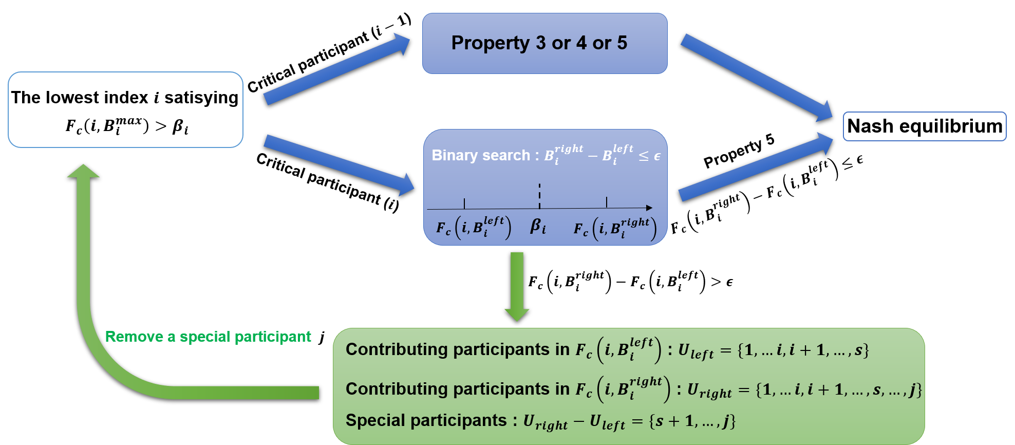
Note that when (refined) CAFL game has a Nash equilibrium with the identified critical participant $c$, we can compute the equilibrium strategies as follows: 1) we set $B_{k}=B^{max}_{k},\forall k\in\{1,...,c-1\};$ 2) $B_{c}=B^{con}_{c}$; 3) obtain the strategies for the participants in the set $\{c+1,...,K^{new}\}$ using Algorithm 2 based on the partial game $G$. Here, $K^{new}$ denotes the total number of participants in the refined CAFL game after removing the special participants if the original CAFL game does not have a Nash equilibrium. For the removed participants, we have $B_{k}=0$ and they are excluded from obtaining the trained FL model.

Due to space limit, more analysis on the above equilibrium construction procedure is detailed in Subsection E in Appendix B in the separate supplementary file.

We first propose our approach to compute a Nash equilibrium for the CAFL game in Algorithm 3, with the key idea of searching the correct critical participant. In Line 1, we first search the critical participant ($i-1$ or $i$) using the binary search. In Lines 2 and 3, if $i-1$ is the critical participant at equilibrium, his strategy must be $B_{i-1}^{max}$. In Lines 6 and 7, we consider the case that $i$ is the critical participant. Line 8 corresponds to Property 5 ($i$ as critical participant). In Line 12, when Property 5 does not hold, we fail in achieving Nash equilibrium. Only one participant with the lowest $\beta_{k}$ in the special participants (obtained in binary search) is removed. In Line 13, we repeat all steps and go to Line 1. We can characterize the convergence of Algorithm 3 in Theorem 7.

The proof is given in Subsection F in Appendix B in the separate supplementary file. We further analyze the complexity of Algorithm 3. We first obtain the complexity for one iteration (Line 1-12). The complexity of calculating $F_{c}(i,B_{i}^{max})$ is $O(K)$. Hence, the complexity of Line 1 is $O(K\log(K))$. In Line 4, constructing equilibrium strategy for each participant, the complexity is $O(K)$. In Line 7, the complexity of binary search is $O(\log(\frac{B^{max}-B_{th}}{\epsilon}))$. Here, $B^{max}=\underset{\forall k\in\mathcal{K}}{\max}(B_{k}^{max})$. Thus, the complexity of one iteration is $O(K\log(\frac{B^{max}-B_{th}}{\epsilon})+K\log(K))$. Based on Theorem 7 (the maximum number of iteration is bounded by $K$), the complexity of Algorithm 3 is $O(K^{2}\log(\frac{B^{max}-B_{th}}{\epsilon})+K^{2}\log(K))$. Note that, a lower $\epsilon$ leads to a higher complexity.

References

- [1] S. Khare and M. Totaro, “Big data in iot,” in 2019 10th International Conference on Computing, Communication and Networking Technologies (ICCCNT), Jul. 2019, pp. 1–7.
- [2] P. Yadav and S. Vishwakarma, “Application of internet of things and big data towards a smart city,” in 2018 3rd International Conference On Internet of Things: Smart Innovation and Usages (IoT-SIU), Feb. 2018, pp. 1–5.
- [3] J. Park, S. Samarakoon, M. Bennis, and M. Debbah, “Wireless network intelligence at the edge,” Proceedings of the IEEE, vol. 107, no. 11, pp. 2204–2239, Nov. 2019.
- [4] J. Xie, Z. Song, Y. Li, Y. Zhang, H. Yu, J. Zhan, Z. Ma, Y. Qiao, J. Zhang, and J. Guo, “A survey on machine learning-based mobile big data analysis: Challenges and applications,” Wireless Communications and Mobile Computing, vol. 2018, pp. 1–19, 2018.
- [5] N. Rastogi, S. K. Singh, and P. K. Singh, “Privacy and security issues in big data: Through indian prospective,” in 2018 3rd International Conference On Internet of Things: Smart Innovation and Usages (IoT-SIU), Feb. 2018, pp. 1–11.
- [6] B. McMahan, E. Moore, D. Ramage, S. Hampson, and B. A. y Arcas, “Communication-efficient learning of deep networks from decentralized data,” in Artificial Intelligence and Statistics, 2017, pp. 1273–1282.
- [7] J. Kang, Z. Xiong, D. Niyato, H. Yu, Y. Liang, and D. I. Kim, “Incentive design for efficient federated learning in mobile networks: A contract theory approach,” in 2019 IEEE VTS Asia Pacific Wireless Communications Symposium (APWCS), Dec. 2019, pp. 1–5.
- [8] S. R. Pandey, N. H. Tran, M. Bennis, Y. K. Tun, Z. Han, and C. S. Hong, “Incentivize to build: A crowdsourcing framework for federated learning,” in 2019 IEEE Global Communications Conference (GLOBECOM), Dec. 2019, pp. 1–6.
- [9] Y. Sarikaya and O. Ercetin, “Motivating workers in federated learning: A stackelberg game perspective,” IEEE Networking Letters, vol. 2, no. 1, pp. 23–27, Mar. 2020.
- [10] N. Ding, Z. Fang, and J. Huang, “Incentive mechanism design for federated learning with multi-dimensional private information,” in 2020 18th International Symposium on Modeling and Optimization in Mobile, Ad Hoc, and Wireless Networks (WiOPT), Jun. 2020, pp. 1–8.
- [11] J. Kang, Z. Xiong, D. Niyato, S. Xie, and J. Zhang, “Incentive mechanism for reliable federated learning: A joint optimization approach to combining reputation and contract theory,” IEEE Internet of Things Journal, vol. 6, no. 6, pp. 10 700–10 714, Dec. 2019.
- [12] Y. Zhan, P. Li, Z. Qu, D. Zeng, and S. Guo, “A learning-based incentive mechanism for federated learning,” IEEE Internet of Things Journal, vol. 7, no. 7, pp. 6360–6368, Jul. 2020.
- [13] T. H. T. Le, N. H. Tran, Y. K. Tun, M. N. H. Nguyen, S. R. Pandey, Z. Han, and C. S. Hong, “An incentive mechanism for federated learning in wireless cellular network: An auction approach,” IEEE Transactions on Wireless Communications, pp. 1–1, 2021.
- [14] Y. Zhan, J. Zhang, Z. Hong, L. Wu, P. Li, and S. Guo, “A survey of incentive mechanism design for federated learning,” IEEE Transactions on Emerging Topics in Computing, pp. 1–1, 2021.
- [15] Y. Hu, D. Niu, J. Yang, and S. Zhou, “Fdml: A collaborative machine learning framework for distributed features,” in Proceedings of the 25th ACM SIGKDD International Conference on Knowledge Discovery & Data Mining, 2019, pp. 2232–2240.
- [16] Q. Wu, X. Chen, Z. Zhou, and J. Zhang, “Fedhome: Cloud-edge based personalized federated learning for in-home health monitoring,” IEEE Transactions on Mobile Computing, pp. 1–1, 2020.
- [17] P. Kairouz, H. B. McMahan, B. Avent et al., “Advances and open problems in federated learning,” arXiv:1912.04977, 2019. [Online]. Available: https://arxiv.org/abs/1912.04977
- [18] J. Ren, G. Yu, and G. Ding, “Accelerating dnn training in wireless federated edge learning system,” arXiv:1905.09712, 2019. [Online]. Available: https://arxiv.org/abs/1905.09712
- [19] N. H. Tran, W. Bao, A. Zomaya, M. N. H. Nguyen, and C. S. Hong, “Federated learning over wireless networks: Optimization model design and analysis,” in IEEE INFOCOM 2019 - IEEE Conference on Computer Communications, 2019, pp. 1387–1395.
- [20] N. Ding, Z. Fang, and J. Huang, “Optimal contract design for efficient federated learning with multi-dimensional private information,” IEEE Journal on Selected Areas in Communications, vol. 39, no. 1, pp. 186–200, 2021.
- [21] L. Zhang, T. Zhu, P. Xiong, W. Zhou, and P. Yu, “A robust game-theoretical federated learning framework with joint differential privacy,” IEEE Transactions on Knowledge and Data Engineering, pp. 1–1, 2022.
- [22] R. Hu and Y. Gong, “Trading data for learning: Incentive mechanism for on-device federated learning,” in GLOBECOM 2020 - 2020 IEEE Global Communications Conference, 2020, pp. 1–6.
- [23] M. Li, T. Zhang, Y. Chen, and A. J. Smola, “Efficient mini-batch training for stochastic optimization,” in Proceedings of the 20th ACM SIGKDD International Conference on Knowledge Discovery and Data Mining, 2014, p. 661–670.
- [24] L. Duan, T. Kubo, K. Sugiyama, J. Huang, T. Hasegawa, and J. Walrand, “Incentive mechanisms for smartphone collaboration in data acquisition and distributed computing,” in 2012 Proceedings IEEE INFOCOM, Mar. 2012, pp. 1701–1709.
- [25] M. Tang and V. W. Wong, “An incentive mechanism for cross-silo federated learning: A public goods perspective,” in IEEE INFOCOM 2021 - IEEE Conference on Computer Communications, 2021, pp. 1–10.
- [26] H. Wang, K. Sreenivasan, S. Rajput, H. Vishwakarma, S. Agarwal, J.-y. Sohn, K. Lee, and D. Papailiopoulos, “Attack of the tails: Yes, you really can backdoor federated learning,” Advances in Neural Information Processing Systems, vol. 33, pp. 16 070–16 084, 2020.
- [27] C. Xie, M. Chen, P.-Y. Chen, and B. Li, “Crfl: Certifiably robust federated learning against backdoor attacks,” in International Conference on Machine Learning. PMLR, 2021, pp. 11 372–11 382.
- [28] S. Andreina, G. A. Marson, H. Möllering, and G. Karame, “Baffle: Backdoor detection via feedback-based federated learning,” in 2021 IEEE 41st International Conference on Distributed Computing Systems (ICDCS), 2021, pp. 852–863.
- [29] C. P. Wan and Q. Chen, “Robust federated learning with attack-adaptive aggregation,” arXiv:2102.05257, 2021. [Online]. Available: https://arxiv.org/abs/2102.05257
- [30] D. Kahneman and A. Tversky, “Prospect theory: An analysis of decision under risk,” in Handbook of the fundamentals of financial decision making: Part I. World Scientific, 2013, pp. 99–127.
- [31] P. A. Apostolopoulos, E. E. Tsiropoulou, and S. Papavassiliou, “Risk-aware data offloading in multi-server multi-access edge computing environment,” IEEE/ACM Transactions on Networking, vol. 28, no. 3, pp. 1405–1418, 2020.
- [32] Y. Lecun, L. Bottou, Y. Bengio, and P. Haffner, “Gradient-based learning applied to document recognition,” Proceedings of the IEEE, vol. 86, no. 11, pp. 2278–2324, 1998.
- [33] H. Xiao, K. Rasul, and R. Vollgraf, “Fashion-mnist: a novel image dataset for benchmarking machine learning algorithms,” arXiv preprint arXiv:1708.07747, 2017.
- [34] A. Krizhevsky, G. Hinton et al., “Learning multiple layers of features from tiny images,” 2009.
- [35] Q. Yang, Y. Liu, T. Chen, and Y. Tong, “Federated machine learning: Concept and applications,” ACM Transactions on Intelligent Systems and Technology (TIST), vol. 10, no. 2, pp. 1–19, 2019.
- [36] X. Li, K. Huang, W. Yang, S. Wang, and Z. Zhang, “On the convergence of fedavg on non-iid data,” arXiv:1907.02189, 2019. [Online]. Available: https://arxiv.org/abs/1907.02189
- [37] L. U. Khan, M. Alsenwi, Z. Han, and C. S. Hong, “Self organizing federated learning over wireless networks: A socially aware clustering approach,” in 2020 International Conference on Information Networking (ICOIN), Jan. 2020, pp. 453–458.
- [38] L. Xu, C. Jiang, J. Wang, Y. Ren, J. Yuan, and M. Guizani, “Game theoretic data privacy preservation: Equilibrium and pricing,” in 2015 IEEE International Conference on Communications (ICC), Jun. 2015, pp. 7071–7076.
- [39] L. U. Khan, N. H. Tran, S. R. Pandey, W. Saad, Z. Han, M. N. H. Nguyen, and C. S. Hong, “Federated learning for edge networks: Resource optimization and incentive mechanism,” arXiv:1911.05642, 2019. [Online]. Available: https://arxiv.org/abs/1911.05642
- [40] W. James N., Game Theory. Springer, 2006.