Machine-checked executable semantics of Stateflow

There have been plenty of works on semantics of Stateflow-like modeling languages. Statecharts, introduced by Harel [8], is a precursor of Stateflow for modelling reactive systems, and its semantics was extensively studied [9, 16, 4]. One version of the semantics in terms of hierarchical automata was formalized in Isabelle/HOL [11]. However, Stateflow is different from Statecharts in several aspects. In particular, the execution of Stateflow is deterministic, due to assignment of priorities to parallel states and transitions, whereas Statecharts is inherently non-deterministic. Hamon presented denotational semantics [6] and operational semantics [7] for a subset of Stateflow. These works provide a basis for later studies. However, they miss some important features of Stateflow such as temporal operators, early return caused by event broadcasts, and so on. Furthermore, the semantics was given as mathematical definitions without formalization in proof assistants. Bourbouh et al. adapted the denotational semantics to continuation-passing style, and used this to implement an interpreter and code generator for Stateflow [1]. Izerrouken et al. formalized a specification of sequencing of Simulink blocks in Coq, as part of the qualification process for the GeneAuto code generator for Simulink [12]. It does not consider semantics for Stateflow.

Stateflow has also been translated to other modelling languages with formal semantics and verification support. Scaife et al. defined a safe subset of Stateflow and described the translation of the subset into Lustre for model checking [17]. Cavalcanti used Circus to specify Stateflow diagrams [2]. Chen et al. translated Stateflow to CSP# for formal analysis using the PAT model checker [3]. Jiang et al. proposed a translation from a subset of Stateflow to UPPAAL for verification [13]. The above work covers a larger subset of Stateflow and has been used on practical case studies. However, they lack a direct formalization of Stateflow semantics, and so the correctness of translation is difficult to guarantee. They also do not consider some of the more complex features in Stateflow, such as exact conditions for early return logic, graphical functions, and messages. This paper builds upon existing work of Zou et al. on translation of Stateflow to Hybrid CSP for verification using hybrid Hoare logic. The correctness of translation is proved using UTP theory [22, 20], but without formalization in a theorem prover. Guo et al. simplified this translation procedure as well as expanding the supported features [5].

Compared with the above works, we define an operational semantics that covers a wider range of important features in Stateflow, including exact conditions for early return logic, graphical functions, and messages. We also formalize the semantics in Isabelle/HOL, together with automatic execution of Stateflow models based on this semantics for validation and practical use.

Fig. 1 shows a Stateflow model for a washing machine. The washing machine has two top-level states: On and Off. The Off state is divided into three substates: Sleep, Ready, and Pending. The On state is divided into two substates: AddWater and Washing. The model has three input events: START, STOP, and SWITCH.

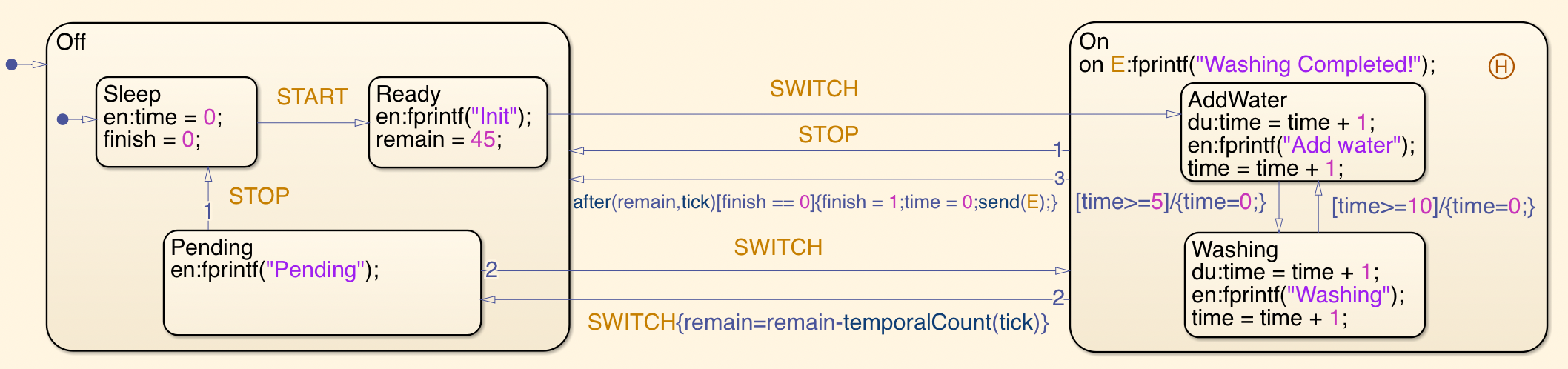
The washing machine starts in state Off and its substate Sleep, as indicated by the default transitions. Variables finish and time are initialized to 0 in the entry action of Sleep. The entry and during actions of a given state are defined after the symbols en and du respectively. Event START triggers a transition from Sleep to Ready, then event SWITCH triggers a transition from Ready to substate AddWater of On. This supertransition, which crosses the state hierarchy, results in exit of both Ready and Off, then entry of both On and its substate AddWater.

When in state On, the washing machine alternates between staying in AddWater for 5 ticks and staying in Washing for 10 ticks. This is controlled by the variable time, which is incremented every tick in both substates, and checked/reset in the transitions between the two substates. There are three transitions from On to Off, two controlled by events and the third by execution cycles. Transition 1 is triggered by STOP to stop the machine. Transition 2 is triggered by SWITCH to pause the machine, updating remain to the remaining working time (initially 45 ticks for the washing duration), and reaches Pending, which can return to state On as soon as SWITCH is received again. A history junction is defined in state On to record the previously active substate of On before pausing the machine, which will be reentered upon receiving SWITCH. Transition 3 is triggered when the washing duration is reached, as indicated by the temporal action $\mathsf{after}(\mathit{remain},\mathsf{tick})$, where $\mathsf{tick}$ is an implicit event in Stateflow representing the execution cycles of the active states. Then, the variable $\mathit{finish}$ is set to 1 (to avoid infinite recursion of transition 3 due to event broadcast of $E$), $\mathit{time}$ is reset to 0, and the local event $E$ is broadcast, which triggers the $\mathsf{on}~E$ action in state On to print the message $\mathtt{Washing~Completed!}$.

When a state becomes active, it is entered first, with the consequence of executing the entry action, then its substates (if any) are entered: all substates for And compositions and the default substate for Or compositions (if there is a history junction, the previously active substate is entered instead). As in the example, when ON is entered again due to switch, the previous substate recorded by the history function is entered.

During the execution of a state, first the outer transitions are checked according to the priority order. If there is one transition path that is able to reach a destination state, a state transition path occurs by exiting the source state, executing the transition actions, and the target state becomes active and is entered. If a terminal junction is reached during the execution, the execution of current state stops. If there is no enabled transition path away from current state, the during and on-event actions of the state executes. Then, the inner transitions of the state is checked in priority order. If still no one is enabled, the active substates inside the current state execute recursively.

When a state needs to be exited, first its substates are exited in the reverse order as they are entered. Then, the exit action of the state is performed.

As seen from the execution of Stateflow states explained above, entry, execution and exit of states are completely deterministic.

We formalize the syntax of Stateflow models as follows. In the syntax, $e$ represents expressions, $b$ Boolean variables, $E$ events, $f$ Matlab functions, and $\mathit{gf}$ graphical functions.

A Stateflow chart $\Gamma$ (called static environment later) consists of the following parts: the state composition $\mathit{root}$ that is the root of all states in the chart; the collection of Matlab functions $F$; the collection of graphical functions $G$, and the collection of junctions $J$. Each Matlab function in $\mathit{fenv}$ has the form $f\mapsto(a,\overline{x},\overline{y})$, where action $a$ is the body of the function, and $\overline{x},\overline{y}$ are the lists of input and output variables. Each graphical function in $\mathit{genv}$ has the form $g\mapsto(t,\overline{z},\overline{r})$, where $t$ is the initial transition, and $\overline{z},\overline{r}$ are lists of input and output variables. Each junction in $\mathit{JDefs}$ has the form $j\mapsto tl$, where $tl$ is the list of outgoing transitions from the junction.

A state composition $\mathit{Comp}$ is either an $\mathsf{And}$-composition of the form $\mathsf{And}(L,\mathit{sf})$, where $L$ is the list of names of substates in priority order, and $\mathit{sf}$ maps names to their definitions, or an $\mathsf{Or}$-composition of the form $\mathsf{Or}(tl,b,\mathit{sf})$, where $tl$ is the list of default transitions, $b$ denotes whether a history junction exists in the composition, and $\mathit{sf}$ maps names of substates to their definitions.

A state definition $sd$ is of the form $(p,a_{i},a_{d},a_{e},tl_{i},tl_{o},C)$, where $p$ is the path to this state, $a_{i},a_{d},a_{e}$ are the entry, during and exit actions, $tl_{i}$ and $tl_{o}$ are the lists of inner and outer transitions in priority order, and $C$ is the internal state composition. A path $p$ is a sequence of state names, possibly ending in a junction name, indicating how to reach the state or junction starting from the root. E.g., the path to state Sleep in Fig. 1 is root.Off.Sleep. $\varepsilon$ represents empty path (or empty transition list in the definition of $tl$). The path to a composition is defined as the path to its parent state.

A transition list $tl$ is an ordered list of transitions. Each transition $t$ has the form $(p_{s},E,c,a_{c},a_{t},p_{d})$, where $p_{s}$ and $p_{d}$ are the source and destination of $t$, $E$ is the event or message guard of the transition, $c$ is the condition, and $a_{c}$ and $a_{t}$ are the condition and transition actions.

We next describe the different actions in Stateflow. The undirected event broadcast $\mathsf{send}(E,b)$ broadcasts event $E$ to the whole chart, while the directed event $\mathsf{send}(E,b,p)$ broadcasts $E$ to state composition given by path $p$. Here parameter $b$ indicates whether the sending event occurs in a transition action, to differentiate the two cases of early return in Fig. 3. Temporal action $\mathsf{on}~tc::a$ means execution of action $a$ is guarded by the temporal condition $tc$; while $\mathsf{on}~E::a$ means $a$ is guarded by the event $E$ or message of name $E$. Calls to Matlab functions and graphical functions are denoted by $f\langle\overline{e}\rangle$ and $\mathit{gf}\langle\langle\overline{e}\rangle\rangle$ respectively. $\mathsf{print}(str)$ prints a string $str$ (in Matlab the function is $\mathsf{fprintf}$). $a_{1};a_{2}$ denotes sequential composition. Other control flow mechanisms, such as if-then-else and loops, are usually defined using flow charts in Stateflow.

Temporal conditions $tc$ can be event-based or absolute time based, with respective intuitive meanings. $E$ in $tc$ is either an event or specified time units. Temporal expression $\mathsf{tempCount}(E)$ counts the number of occurrences of an event, or the number of specified time units, since the activation of the associated state. The syntax for conditions $c$ is as usual, with the addition of temporal conditions.

The configuration of the operational semantics includes two parts: static and dynamic environments. The static environment is simply the Stateflow chart $\Gamma$. The dynamic environment $\alpha$ has the form $(v,I)$, where $v$ contains values of variables, event and timing information, and message lists, and $I$ contains activation status and previously active substate remembered by history junctions.

The valuation $v$ has the form $(vv,ev,tv,mv)$. Here $vv$ maps variables occurring in the chart to their values; $ev$ maps path $p$ and event $e$ to the number of times that $e$ has occurred since the activation of $p$; $tv$ maps path $p$ to the simulation time that has elapsed since the activation of $p$. Finally, $\mathit{mv}$ maps message names to the corresponding message queues. The status $I$ maps each path $p$ (corresponding to a state composition) to its activation status. It consists of whether the given path is active ($\mathit{is\_active}$), the currently active substate ($\mathit{active\_st}$) and previously active substate $\mathit{hj}$ if there is a history junction. For $\mathsf{And}$-compositions, all parallel states become active or inactive together, so the latter two components are not used (always with value $\varepsilon$).

The semantics of expressions $e$ is interpreted over valuations and states, represented by $[\![e]\!]_{v,p}$, which returns the value of $e$ under valuation $v$ and state $p$. Similarly, the semantics for conditions under a given valuation $v$ and a state $p$ is defined by $[\![c]\!]_{v,p}$.

The operational semantics consists of several kinds of arrows whose definitions mutually depend on each other. They range from performing a single action in the chart, to the top-level semantics for handling a sequence of events. We first explain the meaning of each of these arrows. The arrows have some common components: $\Gamma$ in the context is the Stateflow chart, $e$ on the top of the arrow indicates the current triggering event, and $\alpha_{1},\alpha_{2}$ are the starting and ending dynamic environments, respectively. Several arrows take an additional path $p$ in the context. For actions in a state, it is the path to that state; for actions in a transition, it is the path to the source state of the transition path.

• •

  $\Gamma,p\vdash(a,\alpha_{1})\xrightarrow{e}_{\mathit{a}}(\alpha_{2},b)$ means performing action $a$ transforms $\alpha_{1}$ to $\alpha_{2}$, and $b$ is a flag for early return: $b=\bot$ indicates early return has occurred, so the remaining actions should be abandoned, while $b=\top$ indicates early return has not occurred.

• •

  $\Gamma,p\vdash(t,\alpha_{1})\xrightarrow{e}_{\mathit{t}}(\alpha_{2},b,a_{t},ts)$ means performing transition $t$ transforms $\alpha_{1}$ to $\alpha_{2}$, $b$ is the flag for early return, $a_{t}$ the transition action to be accumulated, and $ts$ is the target reached by the transition (either a state or a junction).

• •

  $\Gamma,p\vdash(tl,\alpha_{1})\xrightarrow{e}_{\mathit{tl}}(\alpha_{2},vt,b,\mathit{a_{t}s},ts,hp)$ means exploring a list of transitions $tl$ transforms $\alpha_{1}$ to $\alpha_{2}$, $vt$ indicates whether the transition has successfully reached a state, $b$ is the flag for early return, $\mathit{a_{t}s}$ is the accumulated transition actions, $ts$ is target state reached (if any), and $hp$ is the lowest common ancestor of states and junctions along the transition path. There are three cases for $vt$: 1 means successfully reaching a state; 0 means failing to reach a state, and $-1$ means termination due to reaching a terminal junction.

• •

  $\Gamma\vdash(p,\alpha_{1})\xrightarrow{e}_{\mathit{exS}}(\alpha_{2},b)$ means exiting from state $p$ transforms $\alpha_{1}$ to $\alpha_{2}$, with $b$ the flag for early return. $\Gamma\vdash(p,\alpha_{1})\xrightarrow{e}_{\mathit{exC}}(\alpha_{2},b)$ is the corresponding arrow for exiting from substates of $p$ (the composition of $p$). The arrow $\mathit{exS}$ consists of first performing $\mathit{exC}$, then calling the exit action of $p$ and exiting from $p$ itself.

• •

  $\Gamma,h\vdash(p,\alpha_{1})\xrightarrow{e}_{\mathit{enS}}(\alpha_{2},b)$ means entering state $p$ transforms $\alpha_{1}$ to $\alpha_{2}$, with $b$ the flag for early return. Here $h$ is a path (either $\varepsilon$ or starting from $p$) specifying an eventual target for entry, which is needed to define behavior of supertransitions. $\Gamma,h\vdash(p,\alpha_{1})\xrightarrow{e}_{\mathit{enC}}(\alpha_{2},b)$ is the corresponding arrow for entering substate of $p$ (the composition of $p$). The arrow $\mathit{enS}$ consists of first entering $p$, calling the entry action of $p$, and then performing $\mathit{enC}$.

• •

  $\Gamma,\mathit{is}\vdash(p,\alpha_{1})\xrightarrow{e}_{\mathit{runS}}(\alpha_{2},b)$ means running state $p$ transforms $\alpha_{1}$ to $\alpha_{2}$, with $b$ the flag for early return. Here $\mathit{is}$ indicates whether the current execution is in the process of handling a local event. If yes (i.e. $\mathit{is}=\top$), the simulation time on states will not be incremented. $\Gamma,\mathit{is}\vdash(p,\alpha_{1})\xrightarrow{e}_{\mathit{runC}}(\alpha_{2},b)$ is the corresponding arrow for running substates of $p$ (the composition of $p$).

• •

  $\Gamma\vdash\alpha_{1}\xrightarrow{[e_{1},\cdots,e_{n}]}_{\mathit{Ch}}\alpha_{2}$ is the top-level arrow of the semantics, indicating that handling events $e_{1}$ through $e_{n}$ by the entire chart carries $\alpha_{1}$ to $\alpha_{2}$.

Several additional functions are used in the definition of operational semantics below. $\mathsf{lca}(p_{1},\dots,p_{n})$ is the least common ancestor of paths $p_{1},\dots,p_{n}$. $\mathsf{enb}(t,\alpha,e)$ indicates whether the transition $t$ is enabled from dynamic environment $\alpha$, when the current event is $e$. $\mathsf{state}(\Gamma,p)$ returns the state definition of $p$ under $\Gamma$. $\mathsf{comp}(\Gamma,p)$ returns the composition of $p$ under $\Gamma$. The definitions of these functions are straightforward and are omitted in this paper.

We now show rules for each of the arrows in the operational semantics. For reasons of space we can only show some of the representative rules.

References

- [1] Bourbouh, H., Garoche, P., Garion, C., Gurfinkel, A., Kahsai, T., Thirioux, X.: Automated analysis of Stateflow models. In: LPAR-21. EPiC Series in Computing, vol. 46, pp. 144–161. EasyChair (2017)
- [2] Cavalcanti, A.: Stateflow diagrams in Circus. Electronic Notes in Theoretical Computer Science 240, 23–41 (2009)
- [3] Chen, C., Sun, J., Liu, Y., Dong, J., Zheng, M.: Formal modeling and validation of Stateflow diagrams. The International Journal on Software Tools for Technology Transfer 14(6), 653–671 (2012)
- [4] Eshuis, R.: Reconciling Statechart semantics. Science of Computer Programmin 74(3), 65–99 (2009)
- [5] Guo, P., Zhan, B., Xu, X., Wang, S., Sun, W.: Translating a large subset of Stateflow to hybrid CSP with code optimization. In: SETTA 2021. LNCS, vol. 13071, pp. 3–21. Springer (2021)
- [6] Hamon, G.: A denotational semantics for Stateflow. In: EMSOFT 2005. pp. 164–172. ACM (2005)
- [7] Hamon, G., Rushby, J.: An operational semantics for Stateflow. International Journal on Software Tools for Technology Transfer 9(5-6), 447–456 (2007)
- [8] Harel, D.: Statecharts: A visual formalism for complex systems. Science of Computer Programming 8(3), 231–274 (1987)
- [9] Harel, D., Naamad, A.: The STATEMATE semantics of Statecharts. ACM Transactions on Software Engineering and Methodology 5(4), 293–333 (1996)
- [10] He, J.: From CSP to hybrid systems. In: A Classical Mind, Essays in Honour of C.A.R. Hoare. pp. 171–189. Prentice Hall International (UK) Ltd. (1994)
- [11] Helke, S., Kammüller, F.: Formalizing Statecharts using hierarchical automata. Archive of Formal Proofs (2010)
- [12] Izerrouken, N., Pantel, M., Thirioux, X.: Machine-checked sequencer for critical embedded code generator. In: ICFEM 2009. LNCS, vol. 5885, pp. 521–540. Springer (2009)
- [13] Jiang, Y., Song, H., Yang, Y., Liu, H., Gu, M., Guan, Y., Sun, J., Sha, L.: Dependable model-driven development of CPS: from stateflow simulation to verified implementation. ACM Trans. Cyber Phys. Syst. 3(1), 12:1–12:31 (2019)
- [14] MathWorks: Simulink® User’s Guide (2018a), http://www.mathworks.com/help/pdf_doc/simulink/sl_using.pdf
- [15] MathWorks: Stateflow® User’s Guide (2019a), http://www.mathworks.com/help/pdf_doc/stateflow/sf_ug.pdf
- [16] Mikk, E., Lakhnech, Y., Siegel, M.: Hierarchical automata as model for Statecharts. In: Advances in Computing Science - ASIAN ’97. Lecture Notes in Computer Science, vol. 1345, pp. 181–196. Springer (1997)
- [17] Scaife, N., Sofronis, C., Caspi, P., Tripakis, S., Maraninchi, F.: Defining and translating a "safe" subset of Simulink/Stateflow into Lustre. In: EMSOFT 2004. pp. 259–268. ACM (2004)
- [18] Xu, X., Wang, S., Zhan, B., Jin, X., Talpin, J., Zhan, N.: Unified graphical co-modeling, analysis and verification of cyber-physical systems by combining AADL and Simulink/Stateflow. Theoretical computer science 903, 1–25 (2022)
- [19] Yan, G., Jiao, L., Wang, S., Wang, L., Zhan, N.: Automatically generating systemC code from HCSP formal models. ACM Transactions on Software Engineering and Methodology 29(1), 4:1–4:39 (2020)
- [20] Zhan, N., Wang, S., Zhao, H.: Formal Verification of Simulink/Stateflow Diagrams, A Deductive Approach. Springer (2017)
- [21] Zhou, C., Wang, J., Ravn, A.P.: A formal description of hybrid systems. In: Hybrid Systems. LNCS, vol. 1066, pp. 511–530 (1996)
- [22] Zou, L., Zhan, N., Wang, S., Fränzle, M.: Formal verification of Simulink/Stateflow diagrams. In: ATVA 2015. Lecture Notes in Computer Science, vol. 9364, pp. 464–481. Springer (2015)
Appendix 0.A Executable Semantics in Isabelle
In this section, we give some details about implementation of automatic execution of Stateflow semantics by writing tactics in Isabelle/ML.
We use the case of state execution to illustrate this process. When (rule runS) is applied, it results in a theorem of the form for some dynamic environment . In the implementation, the corresponding ML function is . The function first instantiates the initial environments in the semantic rule, and then calculates and resolves the premises in sequence.
The parameters of the function include the static environment , path to be executed (from which the state is obtained), triggering event , event handling flag , and initial dynamic environment . The implementation can be understood as follows. First, obtain theorem corresponding to the semantics of outer transition, extract the instantiation mappings , and then instantiate the schematic variables in with using built-in function , which returns a concrete theorem with a sequence of premises. Next, calculate the new environment by increasing event occurrences and time of the state, obtain the outer transition theorem by calling with corresponding arguments, and then resolve by eliminating the premise corresponding to to get a new theorem . Following the steps in semantics, next calculate the paths and compositions to exit, and then exit the corresponding composition in , execute the transition actions in , and calculate the paths and compositions to enter, and finally enter the target composition. The state execution completes and returns the final theorem.
Similarly, we can define the functions for executing other semantic rules corresponding to inner transitions and composition of state execution, respectively. Next we give the structure for the definition for executing a state:
As shown above, we first evaluate and execute the outer transition list by calling , from which the transition status is obtained. If is equal to 1 (indicating that some outer transition succeeds to execute), then is called from initial dynamic environment ; otherwise, the inner transition list is executed and the transition status is obtained. If is 1, then is called from , otherwise, is called for executing the composition, which corresponds to rule (runS2) and (runS3) presented in Appendix A.5.
Following the above processes, we implement all the semantic rules in ML, especially is defined for the automatic execution of a Stateflow chart. We define a tactic which calls the main function for automatically executing a chart, to build a theorem corresponding to the above goal.
where is called to build the corresponding theorem for a non-empty goal.