Study of the Roberge-Weiss phase caused by external uniform classical electric field using lattice QCD approach

As introduced, one of our main concerns is whether the imaginary chemical potential, which varies with coordinate $z$, brings about a distribution that varies with $z$ or whether it brings about an overall change. We find that the results depend on the temperature at which the quark matter is located. For $\beta=5.3$ and $\beta=5.64$, $c_{q}(z)$ are shown in Figs. 3 and 4. As can be seen, the chiral condensation rises as the electric field strength increases. The difference is that for lower temperatures, the chiral condensation does not appear to vary with the coordinate $z$. For high temperatures, it is clearly an oscillatory function of $z$. The shape of the function is consistent with a trigonometric function.

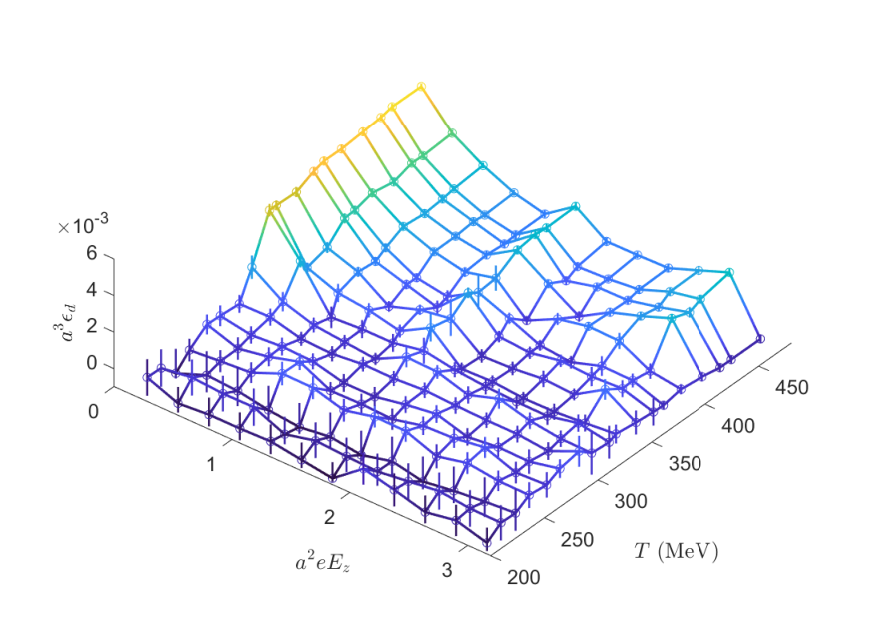
As a signature of whether the chiral condensation varies with $z$, we borrow the definition of standard deviation and define the magnitude of the oscillation of the chiral condensation over $z$, as

where $c_{q}^{T,E_{z}}(z)$ is $c_{q}(z)$ at temperature $T$ and electric field strength $E_{z}$. When $E_{z}=0$, there is no imaginary chemical potential that varies with $z$, therefore $\varepsilon_{q}(T,0)$ are set as baselines, and we define $\epsilon_{q}(T,E_{z})=\varepsilon_{q}(T,E_{z})-\varepsilon_{q}(T,0)$. $\epsilon_{q}$ are shown in Fig. 5. Generally, the amplitude of oscillation grows with temperature. It can also be observed that, for the case of $d$ quark whose electric charge is $-1/3$, the oscillation disappears at $a^{2}eE_{z}=\pi$, for the case of $u$ quark whose electric charge is $2/3$, the oscillation disappears at $a^{2}eE_{z}=\pi/2$ and $a^{2}eE_{z}=\pi$. This can be explained when the frequency of the oscillation is investigated.

Since the linearly changed imaginary chemical potential leads to a periodic change in the partition function, it can be speculated that the chiral condensation that oscillates periodically with the $z$-direction is a reflection of the linearly varying imaginary chemical potential. That is, at high temperatures, the whole system looks more inclined to be a simple combination of $z$-slices corresponding to different imaginary chemical potentials that reach equilibrium independently and then come together. This implies that the chiral condensation located at a certain place does not feel the imaginary chemical potential far away perhaps due to some screening effect and the effect of imaginary chemical potential is therefore a short-range effect on the chiral condensation. On the contrary, when the oscillation disappears, the whole system must be considered as a whole, so that when equilibrium is reached, the chiral condensation located at a certain place can feel the overall distribution of the imaginary chemical potential, and the effect of imaginary chemical potential is therefore a long-range effect on the chiral condensation.

It has been shown , when oscillating, $c_{q}^{T,E_{z}}(z)$ is approximately a trigonometric function. We find that, $c_{q}^{T,E_{z}}(z)$ can be fitted as

where $A_{q}^{T,E_{z}}$ can be viewed as an overall change of the chiral condensation, $B_{q}^{T,E_{z}}$ is the amplitude of oscillation, $f_{c}$ is the frequency of the oscillation.

$c_{q}^{T,E_{z}}(z)$ is fitted according to the ansatz in Eq. (10) using the following steps.

1. 1.

   For a fixed temperature (a fixed $\beta$), choose an initial value for $f_{c}$.

2. 2.

   Find $A_{q}^{E_{z}}$ and $B_{q}^{E_{z}}$ which minimizes the error $\sum_{z}\delta^{2}(q,k,z)$ where $\delta(q,k,z)=A_{q}^{E_{z}^{(k)}}+B_{q}^{E_{z}^{(k)}}\cos(af_{c}zQ_{q}eE_{z}^{(k)})-c_{q}^{E_{z}^{(k)}}(z)$, and $E_{z}^{(k)}=k\pi/12a^{-2}$.

3. 3.

   For $A_{q}^{E_{z}}$ and $B_{q}^{E_{z}}$ obtained in step $2$, find $f_{c}$ which minimize the error $\sum_{q,k,z}\delta^{2}(q,k,z)$.

4. 4.

   Repeat step $2$ and $3$ until $f_{c}$ converges.

5. 5.

   Apply step $2$ for the last time and finish the fit.

The results of the fit depend on the initial value chosen for $f_{c}$, therefore, we fit the case of $a^{2}E_{z}=\pi/12$ for $u$ quark according to the ansatz in Eq. (10) first to set the initial value for $f_{c}$. To ensure reliability, $c_{u}(z)$ at $a^{2}eE_{z}=\pi/2$ and $a^{2}eE_{z}=\pi$, $c_{d}(z)$ at $a^{2}eE_{z}=\pi$ are excluded in the fit.

Taking the case of $\beta=5.64$ for example, $c_{q}^{E_{z}}(z)$ and fitted $c_{q}^{E_{z}}(z)$ are shown in Figs. 6 and 7. Note that the dashed and solid lines are only shown for visual guidance, but not the images of $c_{q}(z)$. In this paper, we use $\chi^{2}/d.o.f.$ to estimate the goodness of fits, which is defined as

where $M$ is the number of points $(x_{i},y_{i})$ participated in the fit, $f(x_{i},\vec{\alpha})$ is the result of fit with $\vec{\alpha}=(\alpha_{1},\alpha_{2},\ldots,\alpha_{N})$ representing the $N$ fit parameters, $\sigma_{i}$ is the statistical error for $y_{i}$.

To ensure reliability, we only fit $c_{q}(z)$ in the regions with strong oscillations. Starting from $\beta=5.46$, $\epsilon_{q}^{T,E_{z}}$ at $a^{2}eE_{z}=\pi/12$ are one order of magnitude larger than the statistical errors of $\epsilon_{q}^{T,E_{z}}$. In the case $\beta\geq 5.46$, we find $\chi^{2}/d.o.f.=0.48\sim 1.07$ for different temperatures.

$A_{q}^{T,E_{z}}$ and $B_{q}^{T,E_{z}}$ are shown in Fig. 8, $f_{c}$ are shown in Fig. 9. It can be observed that, $A_{q}$ grows with $E_{z}$ and decrease with temperature. The overall effect of the electric field on the chiral condensation will be investigated later. Meanwhile, $B_{q}$ is consistent with $\epsilon_{q}$ in Fig. 5. The amplitude of oscillation grows with the temperature and decreases with the electric field strength.

Another interesting and noteworthy conclusion is that $f_{c}\approx 6$ is a constant integer for different flavors at different temperatures and different electric field strengths. This also explained the phenomena that the oscillation disappears for $c_{u}(z)$ at $a^{2}eE_{z}=\pi/2$ and $a^{2}eE_{z}=\pi$, for $c_{d}(z)$ at $a^{2}eE_{z}=\pi$. Since $a^{2}f_{c}Q_{u}eE_{z}=2\pi$ for $a^{2}eE_{z}=\pi/2$ and $4\pi$ for $a^{2}eE_{z}=\pi$, $a^{2}f_{c}Q_{d}E_{z}=-2\pi$ for $a^{2}eE_{z}=\pi$.

The frequency $f_{c}$ actually responds to the $U(1)$ gauge field in Eq. (6). When $k=1$ and $f=6\pi/(L_{z}L_{\tau})=\pi/12$, the flux through the $z-\tau$ plane is $6\pi$, and for quarks, the periods of oscillations along the $z$ coordinate are exactly $Q_{q}\times 6\pi$. Thus, the frequency along $z$ coordinate is actually $f_{c}=L_{\tau}=6$.

It should be pointed out that, so far it is not able to exclude other cases, for example, $f_{c}$ may not be $L_{\tau}$, but $2N_{c}$, or $-2/Q_{d}$, as well as possibly $L_{z}/2$. It will be necessary to use other simulations to finally verify $f_{c}=L_{\tau}$. But we prefer $f_{c}$ to be $L_{\tau}$, and in the following, we use $L_{\tau}$ directly instead of $f_{c}$ to denote the frequency.

The relationship between chiral condensation and the electric field strength is one of the questions of interest in this work. When the system is considered as a whole, $c_{q}$ as functions of $T$ and $E_{z}$ is calculated. The results suffer from strong discretization errors at large $E_{z}$, therefore only the results for $0\leq a^{2}eE_{z}\leq\pi/3$ are presented.

It needs to be kept in mind that the relationship between $c_{q}$ and temperature is not simple, as the renormalization is not applied, it is affected by the relationship between $c_{q}$ and lattice spacing $a$, in addition, as $am_{q}$ is a constant, it is also messed up by the relationship between $c_{q}$ and $m_{q}$ at the same time. Apart from those, the electric field in physical units are different for different $a$, therefore in this subsection, the results are present as functions of $eE_{z}/T^{2}$ instead of $a^{2}eE_{z}$.

Although further verification is needed, it is useful to assume that chiral condensation is still perturbable as the electric field strength varies. In other words, we assume $c_{q}^{T,E_{z}}\approx a_{0}(T)+a_{1}(T)E_{z}^{2}+a_{2}(T)E_{z}^{4}+\ldots$. With this assumption, analytical extension can be applied to obtain the relationship between the chiral condensation and the real electric field strength. The ansatz of $c_{q}^{T,E_{z}}$ up to the order of $E_{z}^{2}$ and $E_{z}^{4}$ are

The results of $c_{u}$ and $c_{d}$ keeping up to $E_{z}^{2}$ are shown in the left panels of Figs. 10 and 11, respectively. The results of $c_{u}$ and $c_{d}$ keeping up to $E_{z}^{4}$ are shown in the left panels of Figs. 12 and 13, respectively. The $\chi^{2}/d.o.f.$ are $7.3$ and $3.2$ for $c_{u}$ and $c_{d}$ keeping up to $E_{z}^{2}$, $2.5$ and $1.9$ for $c_{u}$ and $c_{d}$ keeping up to $E_{z}^{4}$. In our simulation, we use an imaginary electric field strength. To obtain the relationship between $c_{q}$ and $E_{z}$, an analytical extension is applied to rotate the electric field strength back to the real axis. The results of $c_{u}$ and $c_{d}$ keeping up to $E_{z}^{2}$ after analytical extension are shown in the right panels of Figs. 10 and 11, respectively. The results of $c_{u}$ and $c_{d}$ keeping up to $E_{z}^{4}$ after analytical extension are shown in the right panels of Figs. 12 and 13, respectively. Both the ansatz in Eqs. (12) and (13) support the conclusion that the external electric field restores the chiral symmetry as predicted by previous works.

Moreover, since $\left|Q_{u}\right|>\left|Q_{d}\right|$, the effect of the electric field is larger for $c_{u}$ than $c_{d}$. The difference defined as $\Delta=c_{u}-c_{d}$ ($\Delta$ is also $\langle\bar{\psi}\tau_{3}\psi\rangle$ where $\tau_{3}$ is the Pauli matrix) is also calculated and depicted in Fig. 14. It can be seen that, $a^{3}\Delta$ is insensitive to temperature.

It has been pointed out that, in equilibrium, the electric and diffusion forces acting on quarks balance each other, which happens when there is a non-constant charge distribution chargedistrib1; chargedistrib2. The charge density can be defined as $Q_{q}e\bar{q}\gamma_{0}q$, which can be related with $c_{q}^{4}$ defined in Eq. (8). We find that, at high temperatures, the imaginary of $c_{q}^{4}$ shows nontrivial dependence on $z$. As will be explained later, we concentrate on ${\rm Im}[c_{d}^{4}]$. To show the oscillation of ${\rm Im}[c_{d}^{4}]$, $\epsilon_{d}^{4}(T,E_{z})$ is defined as same as $\epsilon_{q}(T,E_{z})$ but with $c_{q}^{T,E_{z}}$ replaced by ${\rm Im}[c_{d}^{4}]$. $\epsilon_{d}^{4}$ is shown in Fig. 15. Starting from $T\approx 300\;{\rm MeV}$, the imaginary of $c_{q}^{4}$ starts to oscillate over $z$ coordinate for $\pi/12\leq a^{2}eE_{z}\leq\pi/3$.

We find that, the frequencies of the oscillation are as same as those of $c_{q}(z)$, i.e., the ${\rm Im}[c_{q}^{4,T,E_{z}}]$ can be fitted with the ansatz,

For $\beta=5.64$, ${\rm Im}\left[c_{q}^{4}(z)\right]$ are shown in Fig. 16. $\chi^{2}/d.o.f.$ are found to be $0.086\sim 0.118$. For $c_{u}^{4}$, the case of $a^{2}eE_{z}=\pi/4$ corresponds to no oscillation, that is the reason why $\epsilon_{d}^{4}$ is used to show the oscillation. In all cases, $A_{q}^{4}<0$. We also find that $|A_{d}^{4}|$ decrease with $E_{z}$.

Another interesting quantity is $c_{q}^{3}$. We find that, at high temperatures and at large $E_{z}$ ($a^{2}eE_{z}=\pi/3$), $c_{u}^{3}(z)$ also oscillates over $z$ ($c_{d}^{3}(z)$ starts to oscillate at a larger $E_{z}$ beyond our scope due the large discretization errors). To verify that the oscillations of $c_{u}^{3}(z)$ along $z$ are not caused by not reaching the equilibrium, for $\beta=5.64$ and $a^{2}eE_{z}=\pi/3$, additional $6000$ trajectories are simulated starting from $T.U.=3000$. The results are shown in Fig. 17. Although $c_{u}^{3}(z)$ has a none trivial distribution, $c_{u}^{3}=0$. The none trivial $c_{u}^{3}(z)$ may indicate a none trivial meson condensation caused by Schwinger mechanism isospincharge. Also, since the case of a large $E_{z}$ is affected by large discretization errors, it is possible that this is a fake phenomenon from discretization errors.

The phase of the Polyakov loop is important to study the R-W transition. It is observed that the phase of the Polyakov loop is also oscillating with $z$, but quite different from the case of chiral condensation, the phase of Polyakov loop is oscillating at lower temperatures. Since a large $E_{z}$ corresponds to a high frequency of oscillation and is not suitable for presentation, we show $P(z)$ only for $a^{2}eE_{z}=\pi/12$, in the complex plane, similar to Ref. pzcomplexplane. The case of $\beta=5.30$ and $\beta=5.64$ are shown in Fig. 19, $\langle P(z)\rangle$ in the complex plane exhibits the shape of a pointed triangle for both low temperature and high temperature.

Similar as $\varepsilon_{q}$ in Eq. (9), we define

$\varepsilon_{arg}$ is shown in Fig. 20. Note that, for high temperatures, there are cases that $\arg\left(\langle P\rangle\right)$ is large while $\varepsilon_{\rm arg}$ is small. For $a^{2}eE_{z}=\pi/2$, $\varepsilon_{\rm arg}$ is small. Those properties will be explained later.

For a lower temperature and a small external electric field, the phase of the Polyakov loop is consistent with the R-W transition. The cases of $\beta=5.3$ and $\beta=5.38$ at $a^{2}eE_{z}=\pi/12$ are shown in Fig. 21. It can be seen that there are plateaus in the $\arg\left(\langle P(z)\rangle\right)$ located at $2n\pi/3$ where $n$ are integers.

Since $a^{2}e\Delta E_{z}=\pi/12$ is large, the widths of the plateaus are narrow. For larger $a^{2}eE_{z}$, the widths of plateaus can be neglected, and $\arg\left(\langle P(z)\rangle\right)$ tends to be a linear function of $zE_{z}$, therefore we assume

By adding integer times of $2\pi$, $\arg\left(\langle P(z)\rangle\right)$ is fitted according to Eq. (17). The results of the fit depend on the manually added $2n\pi$ where $n$ are integers, and to minimize the effect of the manually added $2n\pi$, we fit only for the case of $a^{2}eE_{z}\leq\pi/3$. Taking $\beta=5.3$ and $\beta=5.38$ as examples, $\arg\left(\langle P(z)\rangle\right)$ and fitted $\arg\left(\langle P(z)\rangle\right)$ are shown in Fig. 22.

In the region $5.3\leq\beta\leq 5.38$, $\arg\left(\langle P(z)\rangle\right)$ are fitted, and $f_{\rm arg}$ is shown in Fig. 23. The $\chi^{2}/d.o.f.=6.54\sim 42.7$ for different $\beta$, the worst case is $\beta=5.3$. We find that $f_{\rm arg}\approx-2$ which is a constant integer for different temperatures. This integer also explains the phenomena $\arg\left(\langle P(z)\rangle\right)=0$ and $\varepsilon_{\rm arg}=0$ for $a^{2}eE_{z}=\pi$. However, the case of $a^{2}eE_{z}=\pi/2$ cannot be explained, and will be postponed to section. 3.3.2.

Such behavior fits when $\beta<5.4$. Starting from $\beta=5.4$, the behavior of the phase of Polyakov loop becomes different. As examples, $\arg(\langle P(z)\rangle)$ at $\beta=5.4$ and $\beta=5.64$ and at $a^{2}eE_{z}=\pi/12$ are shown in Fig. 24. It can be seen that, the variation of $\arg(\langle P(z)\rangle)$ is much smaller than the case in Fig. 21.

On the other hand, with growing temperatures the pattern of the $\left|\langle P(z)\rangle\right|$ gradually starts to become clear. Similar as $\epsilon_{q}$, we define

and $\epsilon_{\rm abs}(T,E_{z})=\varepsilon_{\rm abs}(T,E_{z})-\varepsilon_{\rm abs}(T,E_{z}=0)$. $\epsilon_{\rm abs}$ is shown in Fig. 25.

For $\left|\langle P(z)\rangle\right|$, we use the ansatz

Using the method to fit for the chiral condensation, and using Eq. (19), $\left|\langle P(z)\rangle\right|$ is fitted. As an example, the case for $\beta=5.64$ is shown in Fig. 26, the $\chi^{2}/d.o.f.=0.73$. It can be seen that, except for the cases $a^{2}eE_{z}=5\pi/12$ and $a^{2}eE_{z}=7\pi/12$, Eq. (19) roughly describes the pattern of $|\langle P(z)\rangle|$. Similar as the case of chiral condensation, the range of $5.46\leq\beta\leq 5.64$ is considered, and $f_{\rm abs}$ is shown in Fig. 27. Again, we find $f_{\rm abs}\approx 2$ which is a constant integer.

At smaller $E_{z}$, another noteworthy interesting phenomenon is that $\epsilon_{u,d}$ in Fig. 5, $\epsilon_{d}^{4}$ in Fig. 15 and $\epsilon_{\rm abc}$ in Fig. 25 decrease with $E_{z}$ in the small $E_{z}$ region. This behavior implies that, the oscillation suddenly appears at a small none-zero $E_{z}$. It has been pointed out in Refs. chargedistrib1; chargedistrib2 that, physical observables exhibit a discontinuity between $E=0$ and any small $E>0$. Our results can be seen as a support for the above conclusion.

After combining the analysis of the phase of Polyakov and the absolute value of Polyakov loop, we conclude that Polyakov loop is consistent with ansatz

where $C_{q}$ are real numbers (and $C_{d}>0$, $C_{u}\geq 0$ after fit) and $A_{p}$ is a complex number because there are cases that $\arg\left(\langle P\rangle\right)$ is large but $\varepsilon_{\rm arg}$ is small which corresponds to a complex $A_{p}$ and $|A_{p}|\gg C_{q}$.

The ansatz in Eq. (20) counts both the effect from $u$ and $d$ quarks, and is able to describe the following phenomena.

• •

  As shown in the left panel of Fig. 28, for $|A_{p}|\ll C_{q}$ and $C_{u}<C_{d}$ the ansatz describes $\langle P(z)\rangle$ in the complex plane in the left panel of Fig. 19. Similarly, when $|A_{p}|\gg C_{q}$, the ansatz describes the right panel of Fig. 19.

• •

  As shown in the right panel of Fig. 28, for $|A_{p}|\ll C_{q}$ and $C_{u}<C_{d}$, Eq. (20) describes the phenomena in Fig. 21. With $C_{d}>C_{u}$, the effect of $C_{u}$ term becomes small plateaus. Ignoring the plateaus, $f_{\rm arg}=L_{\tau}\times Q_{d}=-2$, which explains the phenomena in Figs. 22 and 23.

• •

  As shown in Fig. 29, when $|A_{p}|>C_{q}$, the phase of the Polyakov loop ranges in $[-\pi,\pi)$, when $|A_{p}|<C_{q}$, the phase of the Polyakov loop ranges in $(-\pi/2,\pi/2)$. With the growth of temperature, $|A_{p}|>C_{q}$, the phase of Polyakov loop when $\beta\geq 5.4$ in Fig. 24 can be explained.

• •

  When $|A_{p}|\gg C_{q}$ and $C_{u}\ll C_{d}$, Eq. (20) describes the oscillation in Fig. 26 and $f_{\rm abs}=|L_{\tau}\times Q_{d}|=2$ in Fig. 27 can be understood. A $C_{u}$ term also explains the discrepancy of the ansatz in Eq. (19) at $a^{2}eE_{z}=5\pi/12$ and $a^{2}eE_{z}=7\pi/12$.

• •

  Apart from that, Eq. (20) also explains the reason that $\varepsilon_{\rm arg}$ is small and $\arg\left(\langle P\rangle\right)\approx 0$ at $a^{2}eE_{z}=\pi/2$. This can be attributed to a real $A_{p}$ which is larger than $C_{u}+C_{d}$.

References

- (1) V. P. Gusynin, V. A. Miransky and I. A. Shovkovy, Catalysis of dynamical flavor symmetry breaking by a magnetic field in (2+1)-dimensions, Phys. Rev. Lett. 73 (1994) 3499 [hep-ph/9405262].
- (2) N. O. Agasian, Phase structure of the QCD vacuum in a magnetic field at low temperature, Phys. Lett. B 488 (2000) 39 [hep-ph/0005300].
- (3) I. A. Shovkovy, Magnetic Catalysis: A Review, Lect. Notes Phys. 871 (2013) 13 [1207.5081].
- (4) G. Cao, Recent progresses on QCD phases in a strong magnetic field: views from Nambu-Jona-Lasinio model, Eur. Phys. J. A 57 (2021) 264 [2103.00456].
- (5) H. T. Ding, S. T. Li, Q. Shi, A. Tomiya, X. D. Wang and Y. Zhang, QCD phase structure in strong magnetic fields, Acta Phys. Polon. Supp. 14 (2021) 403 [2011.04870].
- (6) X.-G. Huang, Electromagnetic fields and anomalous transports in heavy-ion collisions — A pedagogical review, Rept. Prog. Phys. 79 (2016) 076302 [1509.04073].
- (7) A. Y. Babansky, E. V. Gorbar and G. V. Shchepanyuk, Chiral symmetry breaking in the Nambu-Jona-Lasinio model in external constant electromagnetic field, Phys. Lett. B 419 (1998) 272 [hep-th/9705218].
- (8) A. Goyal and M. Dahiya, Chiral symmetry in linear sigma model in magnetic environment, Phys. Rev. D 62 (2000) 025022 [hep-ph/9906367].
- (9) S. P. Klevansky, The Nambu-Jona-Lasinio model of quantum chromodynamics, Rev. Mod. Phys. 64 (1992) 649.
- (10) D. Ebert, K. G. Klimenko, M. A. Vdovichenko and A. S. Vshivtsev, Magnetic oscillations in dense cold quark matter with four fermion interactions, Phys. Rev. D 61 (2000) 025005 [hep-ph/9905253].
- (11) K. G. Klimenko and D. Ebert, Magnetic catalysis of stability of quark matter in the Nambu–Jona-Lasinio model, Phys. Atom. Nucl. 68 (2005) 124.
- (12) G. S. Bali, F. Bruckmann, G. Endrodi, Z. Fodor, S. D. Katz, S. Krieg et al., The QCD phase diagram for external magnetic fields, JHEP 02 (2012) 044 [1111.4956].
- (13) G. S. Bali, F. Bruckmann, G. Endrodi, Z. Fodor, S. D. Katz and A. Schafer, QCD quark condensate in external magnetic fields, Phys. Rev. D 86 (2012) 071502 [1206.4205].
- (14) G. S. Bali, F. Bruckmann, G. Endrodi, F. Gruber and A. Schaefer, Magnetic field-induced gluonic (inverse) catalysis and pressure (an)isotropy in QCD, JHEP 04 (2013) 130 [1303.1328].
- (15) A. Tomiya, H.-T. Ding, S. Mukherjee, C. Schmidt and X.-D. Wang, Chiral phase transition of three flavor QCD with nonzero magnetic field using standard staggered fermions, EPJ Web Conf. 175 (2018) 07041 [1711.02884].
- (16) A. Tomiya, H.-T. Ding, X.-D. Wang, Y. Zhang, S. Mukherjee and C. Schmidt, Phase structure of three flavor QCD in external magnetic fields using HISQ fermions, PoS LATTICE2018 (2019) 163 [1904.01276].
- (17) H.-T. Ding, S.-T. Li, S. Mukherjee, A. Tomiya and X.-D. Wang, Meson masses in external magnetic fields with HISQ fermions, PoS LATTICE2019 (2020) 250 [2001.05322].
- (18) H. T. Ding, S. T. Li, Q. Shi and X. D. Wang, Fluctuations and correlations of net baryon number, electric charge and strangeness in a background magnetic field, Eur. Phys. J. A 57 (2021) 202 [2104.06843].
- (19) H. T. Ding, S. T. Li, J. H. Liu and X. D. Wang, Chiral condensates and screening masses of neutral pseudoscalar mesons in thermomagnetic QCD medium, Phys. Rev. D 105 (2022) 034514 [2201.02349].
- (20) M. D’Elia, Lattice QCD Simulations in External Background Fields, Lect. Notes Phys. 871 (2013) 181 [1209.0374].
- (21) S. Mao, From inverse to delayed magnetic catalysis in a strong magnetic field, Phys. Rev. D 94 (2016) 036007 [1605.04526].
- (22) M. N. Chernodub, QCD string breaking in strong magnetic field, Mod. Phys. Lett. A 29 (2014) 1450162 [1001.0570].
- (23) M. Ferreira, P. Costa, O. Lourenço, T. Frederico and C. Providência, Inverse magnetic catalysis in the (2+1)-flavor Nambu-Jona-Lasinio and Polyakov-Nambu-Jona-Lasinio models, Phys. Rev. D 89 (2014) 116011 [1404.5577].
- (24) J. Chao, P. Chu and M. Huang, Inverse magnetic catalysis induced by sphalerons, Phys. Rev. D 88 (2013) 054009 [1305.1100].
- (25) A. Bazavov et al., Freeze-out Conditions in Heavy Ion Collisions from QCD Thermodynamics, Phys. Rev. Lett. 109 (2012) 192302 [1208.1220].
- (26) K. Fukushima and Y. Hidaka, Magnetic Catalysis Versus Magnetic Inhibition, Phys. Rev. Lett. 110 (2013) 031601 [1209.1319].
- (27) F. Bruckmann, G. Endrodi and T. G. Kovacs, Inverse magnetic catalysis and the Polyakov loop, JHEP 04 (2013) 112 [1303.3972].
- (28) M. A. Nowak, M. Sadzikowski and I. Zahed, Chiral Disorder and Random Matrix Theory with Magnetism, Acta Phys. Polon. B 47 (2016) 2173 [1304.6020].
- (29) L. Yu, H. Liu and M. Huang, Spontaneous generation of local CP violation and inverse magnetic catalysis, Phys. Rev. D 90 (2014) 074009 [1404.6969].
- (30) H. Liu, L. Yu and M. Huang, Charged and neutral vector mesons in a magnetic field, Phys. Rev. D 91 (2015) 014017 [1408.1318].
- (31) H. Liu, X. Wang, L. Yu and M. Huang, Neutral and charged scalar mesons, pseudoscalar mesons, and diquarks in magnetic fields, Phys. Rev. D 97 (2018) 076008 [1801.02174].
- (32) A. Bzdak and V. Skokov, Event-by-event fluctuations of magnetic and electric fields in heavy ion collisions, Phys. Lett. B 710 (2012) 171 [1111.1949].
- (33) W.-T. Deng and X.-G. Huang, Event-by-event generation of electromagnetic fields in heavy-ion collisions, Phys. Rev. C 85 (2012) 044907 [1201.5108].
- (34) J. Bloczynski, X.-G. Huang, X. Zhang and J. Liao, Azimuthally fluctuating magnetic field and its impacts on observables in heavy-ion collisions, Phys. Lett. B 718 (2013) 1529 [1209.6594].
- (35) S. P. Klevansky and R. H. Lemmer, Chiral symmetry restoration in the Nambu-Jona-Lasinio model with a constant electromagnetic field, Phys. Rev. D 39 (1989) 3478.
- (36) H. Suganuma and T. Tatsumi, On the Behavior of Symmetry and Phase Transitions in a Strong Electromagnetic Field, Annals Phys. 208 (1991) 470.
- (37) W. R. Tavares, R. L. S. Farias and S. S. Avancini, Deconfinement and chiral phase transitions in quark matter with a strong electric field, Phys. Rev. D 101 (2020) 016017 [1912.00305].
- (38) G. Cao and X.-G. Huang, Chiral phase transition and Schwinger mechanism in a pure electric field, Phys. Rev. D 93 (2016) 016007 [1510.05125].
- (39) M. Ruggieri, Z. Y. Lu and G. X. Peng, Influence of chiral chemical potential, parallel electric, and magnetic fields on the critical temperature of QCD, Phys. Rev. D 94 (2016) 116003 [1608.08310].
- (40) M. Ruggieri and G.-X. Peng, Chiral phase transition of quark matter in the background of parallel electric and magnetic fields, Nucl. Sci. Tech. 27 (2016) 130.
- (41) A. Yamamoto, Lattice QCD with strong external electric fields, Phys. Rev. Lett. 110 (2013) 112001 [1210.8250].
- (42) P. de Forcrand and O. Philipsen, The QCD phase diagram for small densities from imaginary chemical potential, Nucl. Phys. B 642 (2002) 290 [hep-lat/0205016].
- (43) M. D’Elia and M.-P. Lombardo, Finite density QCD via imaginary chemical potential, Phys. Rev. D 67 (2003) 014505 [hep-lat/0209146].
- (44) E. Shintani, S. Aoki, N. Ishizuka, K. Kanaya, Y. Kikukawa, Y. Kuramashi et al., Neutron electric dipole moment with external electric field method in lattice QCD, Phys. Rev. D 75 (2007) 034507 [hep-lat/0611032].
- (45) A. Alexandru and F. X. Lee, The Background field method on the lattice, PoS LATTICE2008 (2008) 145 [0810.2833].
- (46) M. D’Elia, M. Mariti and F. Negro, Susceptibility of the QCD vacuum to CP-odd electromagnetic background fields, Phys. Rev. Lett. 110 (2013) 082002 [1209.0722].
- (47) H. R. Fiebig, W. Wilcox and R. M. Woloshyn, A Study of Hadron Electric Polarizability in Quenched Lattice QCD, Nucl. Phys. B 324 (1989) 47.
- (48) J. C. Christensen, W. Wilcox, F. X. Lee and L.-m. Zhou, Electric polarizability of neutral hadrons from lattice QCD, Phys. Rev. D 72 (2005) 034503 [hep-lat/0408024].
- (49) LHPC collaboration, Neutron electric polarizability from unquenched lattice QCD using the background field approach, Phys. Rev. D 76 (2007) 114502 [0706.3919].
- (50) G. Endrodi and G. Marko, Thermal QCD with external imaginary electric fields on the lattice, PoS LATTICE2021 (2022) 245 [2110.12189].
- (51) G. Endrődi and G. Markó, On electric fields in hot QCD: perturbation theory, 2208.14306.
- (52) A. Roberge and N. Weiss, Gauge Theories With Imaginary Chemical Potential and the Phases of QCD, Nucl. Phys. B 275 (1986) 734.
- (53) O. Philipsen and C. Pinke, Nature of the Roberge-Weiss transition in QCD with Wilson fermions, Phys. Rev. D 89 (2014) 094504 [1402.0838].
- (54) M. D’Elia and M. Mariti, Effect of Compactified Dimensions and Background Magnetic Fields on the Phase Structure of SU(N) Gauge Theories, Phys. Rev. Lett. 118 (2017) 172001 [1612.07752].
- (55) J. Samuel, Wick Rotation in the Tangent Space, Class. Quant. Grav. 33 (2016) 015006 [1510.07365].
- (56) J. B. Kogut and L. Susskind, Hamiltonian Formulation of Wilson’s Lattice Gauge Theories, Phys. Rev. D 11 (1975) 395.
- (57) C. Gattringer and C. B. Lang, Quantum chromodynamics on the lattice, vol. 788. Springer, Berlin, 2010, 10.1007/978-3-642-01850-3.
- (58) K. G. Wilson, Confinement of Quarks, Phys. Rev. D 10 (1974) 2445.
- (59) P. H. Damgaard and U. M. Heller, The U(1) Higgs Model in an External Electromagnetic Field, Nucl. Phys. B 309 (1988) 625.
- (60) M. H. Al-Hashimi and U. J. Wiese, Discrete Accidental Symmetry for a Particle in a Constant Magnetic Field on a Torus, Annals Phys. 324 (2009) 343 [0807.0630].
- (61) P. V. Buividovich, M. N. Chernodub, E. V. Luschevskaya and M. I. Polikarpov, Lattice QCD in strong magnetic fields, eCONF C0906083 (2009) 25 [0909.1808].
- (62) S. Ueda, S. Aoki, T. Aoyama, K. Kanaya, H. Matsufuru, S. Motoki et al., Development of an object oriented lattice QCD code ’Bridge++’, J. Phys. Conf. Ser. 523 (2014) 012046.
- (63) B. Orth, T. Lippert and K. Schilling, Finite-size effects in lattice QCD with dynamical Wilson fermions, Phys. Rev. D 72 (2005) 014503 [hep-lat/0503016].
- (64) TXL, T(X)L collaboration, Static potentials and glueball masses from QCD simulations with Wilson sea quarks, Phys. Rev. D 62 (2000) 054503 [hep-lat/0003012].
- (65) G. S. Bali and K. Schilling, Static quark - anti-quark potential: Scaling behavior and finite size effects in SU(3) lattice gauge theory, Phys. Rev. D 46 (1992) 2636.
- (66) R. Sommer, A New way to set the energy scale in lattice gauge theories and its applications to the static force and alpha-s in SU(2) Yang-Mills theory, Nucl. Phys. B 411 (1994) 839 [hep-lat/9310022].
- (67) M. Cheng et al., The QCD equation of state with almost physical quark masses, Phys. Rev. D 77 (2008) 014511 [0710.0354].
- (68) MILC collaboration, Results for light pseudoscalar mesons, PoS LATTICE2010 (2010) 074 [1012.0868].
- (69) ALPHA collaboration, Monte Carlo errors with less errors, Comput. Phys. Commun. 156 (2004) 143 [hep-lat/0306017].
- (70) A. Bazavov et al., The chiral and deconfinement aspects of the QCD transition, Phys. Rev. D 85 (2012) 054503 [1111.1710].