跳到论文正文
W Papers独立论文阅读器 arXiv:2207.11392 论文正文 计算阅读时间 · 0%
引用这篇论文根据当前论文元数据生成,正式投稿前建议核对。


License: arXiv.org perpetual non-exclusive license
arXiv:2207.11392v3 [stat.ME] 27 Apr 2026

Simultaneous Inference for Time Series Functional Linear Regression

Yan Cui Affiliation: Department of Mathematics, Illinois State University, Normal, IL, U.S.    Zhou Zhou Affiliation: Department of Statistical Sciences, University of Toronto, Toronto, ON, Canada
Abstract

We consider the problem of joint simultaneous confidence band (JSCB) construction for regression coefficient functions of time series scalar-on-function linear regression when the regression model is estimated by a roughness penalization approach with flexible choices of orthonormal basis functions. A simple and unified multiplier bootstrap methodology is proposed for the JSCB construction which is shown to achieve the correct coverage probability asymptotically. Furthermore, the JSCB is asymptotically robust to inconsistently estimated standard deviations of the model. The proposed methodology is applied to a time series data set of electricity demands to visually investigate and formally test the overall regression relationship, as well as perform model validation.

Abstract

Section A of this supplemental material discusses several important aspects related to the main article, including the effects of pre-smoothing, practical choices of the basis functions and extensions to regression models with functional response. Section B provides additional simulation results under various numbers of predictors and data generating mechanisms. In Section C, we establish a Gaussian approximation theory for the roughness penalization estimation method, which may be of independent interest. Examples on calculations of the physical dependence measure for a class of functional MA(∞)(\infty) models and a class of functional AR(1) models are presented in Section D. Additional theoretical results, together with proofs of all main results, are provided in Section E.

Keywords: Convex Gaussian approximation; Functional time series; Joint simultaneous confidence band; Multiplier bootstrap; Roughness penalization.

1 Introduction

Modern data collection technologies routinely produce high-frequency time series with complex functional structure, where each observation consists of an entire curve recorded over a time interval. Examples arising in contemporary data science applications include electricity demand curves measured across a day, environmental monitoring data such as pollution or temperature profiles, biomedical signals, and financial intraday curves. To address the resulting statistical issues, functional (or curve) time series analysis has undergone unprecedented development over the last two decades. See [30] and [6] for excellent book-length treatments of the topic. We also refer the readers to [27], [3, 2], [46], [45] and [17], among many others, for articles that address various modelling, estimation, forecasting and inference aspects of functional time series analysis from both time and spectral domain perspectives.

The main purpose of this article is to perform simultaneous statistical inference for time series scalar-on-function linear regression. Specifically, consider the following time series functional linear model (FLM):

Yi=β0+∑j=1p∫01βj(t)Xi​j(t)dt+ϵi,i=1,…,n,Y_{i}=\beta_{0}+\sum_{j=1}^{p}\int_{0}^{1}\beta_{j}(t)X_{ij}(t)\mathrm{d}t+\epsilon_{i},~~i=1,...,n, (1)

where {𝑿i(t):=(Xi​1(t),…,Xi​p(t))⊤}i=1n\{\bm{X}_{i}(t):=(X_{i1}(t),...,X_{ip}(t))^{\top}\}_{i=1}^{n} is a pp-variate stationary time series of known functional predictors observed on [0,1][0,1], {Yi}i=1n\{Y_{i}\}_{i=1}^{n} is a univariate stationary time series of responses, and {ϵi}i=1n\{\epsilon_{i}\}_{i=1}^{n} is a centered stationary time series of regression errors satisfying 𝔼⁡[Xi​j​(t)​ϵi]=0\mathbb{E}[X_{ij}(t)\epsilon_{i}]=0 for all t∈[0,1]t\in[0,1] and j=1,2,…,pj=1,2,...,p. Observe that 𝑿i​(t)\bm{X}_{i}(t) and ϵi\epsilon_{i} could be dependent and β0+∑j=1p∫01βj​(t)​Xi​j​(t)​𝑑t\beta_{0}+\sum_{j=1}^{p}\int_{0}^{1}\beta_{j}(t)X_{ij}(t)\mathrm{d}t can be viewed as the best linear forecast of YiY_{i} based on 𝑿i​(t)\bm{X}_{i}(t). Despite the rapid development of estimation and forecasting methods for functional time series, rigorous statistical inference remains largely underdeveloped, especially for FLMs like (11) involving functional predictors under temporal dependence. Therefore, we are interested in constructing asymptotically correct joint simultaneous confidence bands (JSCB) for the regression coefficients 𝜷⁡(t):=(β1​(t),…,βp​(t))⊤\bm{\beta}(t):=(\beta_{1}(t),...,\beta_{p}(t))^{\top}; that is, we aim to find random functions Ln,j​(t)L_{n,j}(t) and Un,j​(t)U_{n,j}(t), j=1,2,…,pj=1,2,...,p, such that

limn→∞ℙ(Ln,j(t)≤βj(t)≤Un,j(t),for all t∈[0,1]and j=1,2,…,p)=1−α\lim_{n\rightarrow\infty}\mathbb{P}\Big(L_{n,j}(t)\leq\beta_{j}(t)\leq U_{n,j}(t),~\mbox{for all }t\in[0,1]~\mbox{and }j=1,2,...,p\Big)=1-\alpha

for a pre-specified coverage probability 1−α1-\alpha. The need for JSCB arises in many situations when one wants to, for instance, rigorously investigate the overall magnitude and pattern of the regression coefficient functions, test various assumptions on the regression relationship and perform diagnostic checking and model validation of (11) without multiple hypothesis testing problems.

1.1 Main contribution

To better understand the main contributions of this paper, we start by emphasizing that there are two major challenges involved in the JSCB construction of 𝜷⁡(t)\bm{\beta}(t) for the time series FLM (11). First, the estimation of model (11) is related to an ill-posed inverse problem [10, Section 2.2] and estimators of 𝜷⁡(t)\bm{\beta}(t) are typically not tight on [0,1][0,1]. As a result, it has been a difficult and open problem to investigate the large sample distributional behavior of estimators of 𝜷⁡(t)\bm{\beta}(t) uniformly across tt. Second, the rates of convergence for various estimators of 𝜷⁡(t)\bm{\beta}(t) are sensitive to the smoothness of 𝑿i​(t)\bm{X}_{i}(t) and 𝜷⁡(t)\bm{\beta}(t), and the penalization parameter used in the regression. Consequently, in practice it is challenging to determine convergence rates of the estimated coefficient functions and hence the appropriate normalizing constants for uniform inference of 𝜷⁡(t)\bm{\beta}(t).

To address the aforementioned challenges, this article makes two principal contributions. First, we develop a uniform Gaussian approximation theory and comparison results over all Euclidean convex sets for the sum of stationary and weakly dependent time series in moderately high-dimensional settings. To the best of our knowledge, this presents a novel theoretical advancement as such results have not previously been investigated within the contexts of functional time series or functional data. Our findings extend the corresponding results established for independent or mm-dependent data, as explored in [5], [21], and among others. Specifically, the uniform convex Gaussian approximation theory is established for a weighted maximum deviation uniformly over all quantiles and a wide class of weight functions (c.f. Theorem 1 in the supplemental material). Additionally, we derive the explicit comparison bounds on the Kolmogorov distance between the sum of moderately high-dimensional Gaussian vectors, which plays a crucial role in validating the use of multiplier bootstrap procedures. These contributions significantly broaden the range of problems that can be rigorously addressed within functional time series analysis, and offer practical tools for addressing inferential challenges in both functional data and time series domains.

Second, we propose a simple and unified multiplier bootstrap procedure for constructing asymptotically correct JSCBs for 𝜷⁡(t)\bm{\beta}(t). Leveraging the fact that the convex Gaussian approximation and Gaussian comparison results hold uniformly over all Euclidean convex sets, our approach circumvents the need to explicitly derive the limiting distribution of the corresponding maximum deviation or the convergence rates, which are often analytically intractable or extremely difficult to estimate accurately in time-dependent settings. Considering the roughness penalized estimators of 𝜷⁡(t)\bm{\beta}(t) for instance, we demonstrate that the multiplier bootstrap accurately approximates their weighted maximum deviations on [0,1][0,1] uniformly across all quantiles and a wide class of smooth weight functions under quite general conditions in large samples (c.f. Theorem 1 in Section 5.2). Furthermore, the constructed JSCBs remain asymptotically correct even when the weight function is estimated inconsistently under some mild conditions, thereby adding an additional layer of robustness to the proposed methodology. The multiplier bootstrap procedure is easy to implement and practically useful, offering a powerful and versatile tool for empirical studies. To the best of our knowledge, this is the first work to provide JSCBs for FLM under general time series dependence, thereby filling an important gap in uncertainty quantification of functional time series analysis.

1.2 Literature review

To date, results for the time series scalar-on-function regression (11) are scarce and mainly focus on the consistency of functional principal component (FPC) based estimators [27, 26]. To our best knowledge, there is no existing literature on the asymptotically correct JSCB construction for 𝜷⁡(t)\bm{\beta}(t) under time series dependence. On the other hand, there is a wealth of statistics literature dealing with estimation, convergence rates, prediction, and application of FLM (11) when the data {(Yi,𝑿i​(t))}i=1n\{(Y_{i},\bm{X}_{i}(t))\}_{i=1}^{n} are independent and identically distributed (i.i.d.). See, for instance, [9], [16], [36], [8] and [32] for a far from exhaustive list of references. In parallel with the FPC based estimators, [64], developed a Reproducing Kernel Hilbert Space based approach for estimating the slope coefficient function in FLMs. Subsequent studies on minimax convergence rates, prediction, and statistical inference include [7], [53], [18], among others. We also refer the readers to [10], [42], [59] and [49] for excellent recent reviews of the topic and more references.

Meanwhile, the last two decades also witnessed an increase in statistics literature on the inference of FLM (11) for i.i.d. data. Since a JSCB is primarily an inferential tool, we shall review this literature in more detail. The main body of the aforementioned literature consists of results related to ℒ2{\cal L}^{2}-type tests on whether 𝜷⁡(t)=0\bm{\beta}(t)=0 or a fixed known function; see for instance [25], [35], [33] and [55], among others. Other contributions include confidence interval construction for the conditional mean and hypothesis testing for functional contrasts [53] and goodness of fit tests for (11) versus possibly nonlinear alternatives [29, 22, 40]. In contrast, for independent observations, there appear to be few results in the literature discussing the construction of confidence bands for 𝜷⁡(t)\bm{\beta}(t). [31] proposed a simple methodology to construct a conservative confidence band for the slope function of scalar-on-function linear regression aiming at covering “most” of the points with a prespecified probability for independent data. Recently, [18] constructed an asymptotically correct simultaneous confidence band for function-on-function linear regression of independent data, and the authors also discussed the scalar-on-function case briefly. However, the implementation of the latter paper requires estimating the convergence rate of the regression, which could be a relatively difficult task in moderate samples.

On the other hand, the multiplier bootstrap technique has attracted much attention recently. Among others, [11] derived asymptotic consistency of the generalized bootstrap technique for estimating equations. [39] established the validity of the weighted bootstrap technique based on a weighted MM-estimation framework. Later, [54] considered a multiplier bootstrap procedure in the construction of likelihood-based confidence sets under possible model misspecification. Non-asymptotic results on the multiplier bootstrap have been used for high dimensional inference on hyper-rectangles and certain classes of simple convex sets that can be well approximated by (possibly higher dimensional) hyper-rectangles after linear transformations; see for instance [14] and [13] for independent data and [67] for functional time series.

The paper is organized as follows. In Section E.5, we propose the methodology of the JSCB construction based on a roughness penalization approach. Section 3 investigates finite sample accuracy of the bootstrap methodology for various basis functions and weighting schemes using Monte Carlo experiments. We analyze a time series dataset on electricity demand curves and daily total demand in Spain in Section 4. The theoretical result on the multiplier bootstrap for roughness penalized estimators of 𝜷⁡(t)\bm{\beta}(t) is discussed in Section 5. Additional discussions, simulations, examples, theoretical results and the proofs of all theoretical results are deferred to the supplemental material. Reproducible code for the implementation of the JSCB construction is available at https://github.com/YC-stats/FLM_numerical.

2 Methodology

Hereafter, for simplicity we shall assume that YiY_{i} and 𝑿i​(t)\bm{X}_{i}(t) are centered and hence β0=0\beta_{0}=0. Let H=ℒ2​([0,1])H=\mathcal{L}^{2}([0,1]) be the Hilbert space of all square integrable functions on [0,1][0,1] with inner product ⟨x,y⟩=∫01x⁡(t)​y​(t)​𝑑t\langle x,y\rangle=\int_{0}^{1}x(t)y(t)\mathrm{d}t. We also denote by 𝒞d​([0,1])\mathcal{C}^{d}([0,1]) the collection of functions that are dd-times continuously differentiable with absolutely continuous dd-th derivative on [0,1][0,1]. The notation Std⁡(Z){\rm Std}(Z) stands for the standard deviation of a random variable ZZ. Without further specifications, the constants Ci,i=1,2,…C_{i},i=1,2,... are all independent of nn.

2.1 Roughness Penalization Estimation

In order to facilitate the formulation of roughness penalization estimation, we first introduce some notation. Throughout this paper, we assume that Xi​j​(t)X_{ij}(t) for j=1,…,p,i=1,…,nj=1,...,p,~i=1,...,n is continuous on [0,1][0,1] a.s. and hence admits the expansion Xi​j​(t)=∑k=1∞x~i​j,k​αk​(t),X_{ij}(t)=\sum_{k=1}^{\infty}\widetilde{x}_{ij,k}\alpha_{k}(t), where {αk​(t)}k=1∞\{\alpha_{k}(t)\}_{k=1}^{\infty} is a set of pre-selected orthonormal basis functions of HH. From Theorem 1 of [52], Xi​j​(t)X_{ij}(t) has the standard Karhunen-Loève type expansion,

Xi​j​(t)=∑k=1∞fj​k​xi​j,k​αk​(t),X_{ij}(t)=\sum_{k=1}^{\infty}f_{jk}x_{ij,k}\alpha_{k}(t), (2)

where fj​k=Std⁡(x~i​j,k)f_{jk}={\rm Std}(\widetilde{x}_{ij,k}) is the standard deviation of x~i​j,k\widetilde{x}_{ij,k} and xi​j,k=x~i​j,k/fj​kx_{ij,k}=\widetilde{x}_{ij,k}/f_{jk} if fj​k≠0f_{jk}\neq 0. Set xi​j,k=0x_{ij,k}=0 if fj​k=0f_{jk}=0. Notice that fj​kf_{jk} captures the decay speed of x~i​j,k\widetilde{x}_{ij,k} as kk increases and the random coefficient {xi​j,k}k=1∞\{x_{ij,k}\}_{k=1}^{\infty} remains at the same magnitude with variance 11 as kk increases when fj​k≠0f_{jk}\neq 0. Similarly, one can write βj​(t)=∑k=1∞βj​k​αk​(t).\beta_{j}(t)=\sum_{k=1}^{\infty}\beta_{jk}\alpha_{k}(t).

The roughness penalization approach to the FLM (11) is designed to deal with a penalized least squares problem. Following the method proposed by [48], we truncate the number of coefficient functions to finite (but diverging) dimensional spans of a priori set of basis functions {αk​(t)}k=1∞\{\alpha_{k}(t)\}_{k=1}^{\infty} and involves a roughness penalty to obtain an estimator of 𝜷⁡(t)\bm{\beta}(t). Specifically, define the truncated basis expansion of the coefficient function βj​(t)\beta_{j}(t) as βj,cj,n​(t):=∑k=1cj,nβj​k​αk​(t)\beta_{j,c_{j,n}}(t):=\sum_{k=1}^{c_{j,n}}\beta_{jk}\alpha_{k}(t) for j=1,…,pj=1,...,p with the truncation number cj,n→∞c_{j,n}\rightarrow\infty. We consider the penalty term λ​∑j=1p∫01[βj′′​(t)]2​𝑑t\lambda\sum_{j=1}^{p}\int_{0}^{1}[\beta_{j}^{\prime\prime}(t)]^{2}\mathrm{d}t throughout the paper and denote the total truncation number as cn=∑j=1pcj,nc_{n}=\sum_{j=1}^{p}c_{j,n}. Furthermore, let 𝜽c\bm{\theta}_{c} be a cnc_{n}-dimensional block vector where 𝜽j,cn=(θj​1,…,θj​cj,n)⊤\bm{\theta}_{j,c_{n}}=(\theta_{j1},...,\theta_{jc_{j,n}})^{\top} is the jj-th block with θj​k=fj​k​βj​k\theta_{jk}=f_{jk}\beta_{jk} for k=1,…,cj,nk=1,...,c_{j,n}, then the penalized least squares estimator becomes

𝜽~c=[𝑿c⊤​𝑿cn+𝑹⁡(λ)]−1​𝑿c⊤​𝒀n,\widetilde{\bm{\theta}}_{c}=\left[\frac{\bm{X}_{c}^{\top}\bm{X}_{c}}{n}+\bm{R}(\lambda)\right]^{-1}\frac{\bm{X}_{c}^{\top}\bm{Y}}{n},

where 𝒀=(Y1,…,Yn)⊤\bm{Y}=(Y_{1},...,Y_{n})^{\top}, 𝑿c\bm{X}_{c} is an n×cnn\times c_{n} block design matrix with its jjth row (xj​1,1,…,xj​1,c1,n,…,xj​p,1,…,xj​p,cp,n)(x_{j1,1},\ldots,x_{j1,c_{1,n}},\\ \ldots,x_{jp,1},\ldots,x_{jp,c_{p,n}}). The penalty term 𝑹⁡(λ)\bm{R}(\lambda) is a cn×cnc_{n}\times c_{n} block diagonal matrix with λ​𝑹j\lambda\bm{R}_{j} as its diagonals, and 𝑹j\bm{R}_{j} is a cj,n×cj,nc_{j,n}\times c_{j,n} matrix with its (k,l)(k,l)th element Rj​(k,l)=∫01αk′′​(t)​αl′′​(t)​𝑑t/(fj​k​fj​l)R_{j}(k,l)=\int_{0}^{1}\alpha_{k}^{\prime\prime}(t)\alpha_{l}^{\prime\prime}(t)\mathrm{d}t/(f_{jk}f_{jl}). We refer readers to Section D.2 of the supplemental material for further details of the roughness penalization approach. Consequently, the roughness penalized estimator is given by 𝜷~​(t)=𝑪f​(t)​𝜽~c,\widetilde{\bm{\beta}}(t)=\bm{C}_{f}(t)\widetilde{\bm{\theta}}_{c}, where 𝑪f​(t)∈ℝp×cn\bm{C}_{f}(t)\in\mathbb{R}^{p\times c_{n}} is a block-sparse matrix whose jj-th row contains (α1​(t)/fj​1,…,αcj,n​(t)/fj​cj,n)(\alpha_{1}(t)/f_{j1},...,\alpha_{c_{j,n}}(t)/f_{jc_{j,n}}) in columns (j−1)​cj,n+1(j-1)c_{j,n}+1 to j​cj,njc_{j,n}, and zeros elsewhere for j=1,…,pj=1,...,p.

2.2 JSCB Construction

JSCB construction of 𝜷⁡(t)\bm{\beta}(t) boils down to evaluating the distributional behavior of the weighted maximum deviation

Ξn,𝒈n:=n​supt∈[0,1]|𝜷~​(t)−𝜷⁡(t)|𝒈n​(t),\Xi_{n,\bm{g}_{n}}:=\sqrt{n}\sup_{t\in[0,1]}|\widetilde{\bm{\beta}}(t)-\bm{\beta}(t)|_{\bm{g}_{n}(t)},

where |𝑽⁡(t)|𝒈⁡(t)=max1≤j≤p⁡|Vj​(t)/gj​(t)||\bm{V}(t)|_{\bm{g}(t)}=\max_{1\leq j\leq p}|V_{j}(t)/g_{j}(t)| for any function 𝑽⁡(t)=(V1​(t),…,Vp​(t))⊤\bm{V}(t)=(V_{1}(t),...,V_{p}(t))^{\top} and weight function 𝒈⁡(t)=(g1​(t),…,gp​(t))⊤\bm{g}(t)=(g_{1}(t),...,g_{p}(t))^{\top}. The weight function 𝒈n​(t)\bm{g}_{n}(t) is assumed to belong to a class 𝒢\mathcal{G} with

𝒢\displaystyle\mathcal{G} ={𝒇(t):[0,1]→ℝp,𝒇=(f1,…,fp)⊤is a continuousp-dimensional\displaystyle=\{\bm{f}(t):[0,1]\to\mathbb{R}^{p},~\bm{f}=(f_{1},...,f_{p})^{\top}~\text{is a continuous}~p\text{-dimensional}
 vector function satisfyinginft∈[0,1]min1≤j≤pfj(t)≥κ for some constantκ>0}.\displaystyle\text{~vector~function~satisfying}\inf_{t\in[0,1]}\min_{1\leq j\leq p}f_{j}(t)\geq\kappa\text{~for some constant}~\kappa>0\}.

For a given α∈(0,1)\alpha\in(0,1), denote by ξn,𝒈n​(α)\xi_{n,\bm{g}_{n}}(\alpha) the (1−α)(1-\alpha)-th quantile of Ξn,𝒈n\Xi_{n,\bm{g}_{n}}. Then a JSCB with coverage probability 1−α1-\alpha can be constructed as β~j​(t)±ξn,𝒈n​(α)​gn​j​(t)/n\widetilde{\beta}_{j}(t)\pm\xi_{n,\bm{g}_{n}}(\alpha)g_{nj}(t)/\sqrt{n}, t∈[0,1]t\in[0,1], j=1,2,…,pj=1,2,...,p.

Observe that the width of the JSCB is proportional to the weight function 𝒈n​(t)\bm{g}_{n}(t). In practice one could simply choose some fixed weight functions such as gn​j​(t)≡1g_{nj}(t)\equiv 1 which yields equal JSCB width at each tt and jj. Alternatively, when the sample size is sufficiently large and temporal dependence is weak or moderately strong, we recommend choosing gn​j(t)=Std(β~j(t))/∫01Std(β~j(s))ds,j=1,…,p.g_{nj}(t)={\rm Std}(\widetilde{\beta}_{j}(t))/\int_{0}^{1}{\rm Std}(\widetilde{\beta}_{j}(s))\mathrm{d}s,~j=1,...,p. There are two advantages to this data-driven choice of weights. First, the resulting width of the JSCB reflects the standard deviation of 𝜷~​(t)\widetilde{\bm{\beta}}(t) which gives direct visual information on the estimation uncertainty at every t∈[0,1]t\in[0,1] and j=1,…,pj=1,...,p. Second, this choice of weight function yields much smaller average width of the JSCB compared to some fixed choices such as 𝒈n​(t)≡1\bm{g}_{n}(t)\equiv 1; see our simulations in Section 3 for a finite-sample illustration. On the other hand, Std​(β~j​(t)){\rm Std}(\widetilde{\beta}_{j}(t)) has to be estimated in practice. Later in this article, we shall discuss its estimation and also asymptotic robustness of our multiplier bootstrap methodology when the weight function is inconsistently estimated.

To motivate the multiplier bootstrap, denote 𝚺~c​(λ)=𝑿c⊤​𝑿c/n+𝑹⁡(λ)\widetilde{\bm{\Sigma}}_{c}(\lambda)=\bm{X}_{c}^{\top}\bm{X}_{c}/n+\bm{R}(\lambda). For simplicity, we assume that each βj​(t)\beta_{j}(t) has the same degree of smoothness, thereby we let each cj,nc_{j,n} have the same rate of divergence. By elementary calculations and basis expansions, we have

𝜷~​(t)−𝜷⁡(t)=𝑪f​(t)​𝚺~c−1​(λ)​𝑿c⊤​ϵ~n−𝑪f​(t)​𝚺~c−1​(λ)​𝑹​(λ)​𝜽cn+𝒪⁡(cn−d1),\widetilde{\bm{\beta}}(t)-\bm{\beta}(t)=\bm{C}_{f}(t)\widetilde{\bm{\Sigma}}_{c}^{-1}(\lambda)\frac{\bm{X}_{c}^{\top}\widetilde{\bm{\epsilon}}}{n}-\bm{C}_{f}(t)\widetilde{\bm{\Sigma}}_{c}^{-1}(\lambda)\bm{R}(\lambda)\bm{\theta}_{c_{n}}+\mathcal{O}(c_{n}^{-d_{1}}), (3)

where ϵ~=(ϵ1+𝒪ℙ​(cn−(d1+d2+1)),…,ϵn+𝒪ℙ​(cn−(d1+d2+1)))⊤\widetilde{\bm{\epsilon}}=(\epsilon_{1}+\mathcal{O}_{\mathbb{P}}(c_{n}^{-(d_{1}+d_{2}+1)}),...,\epsilon_{n}+\mathcal{O}_{\mathbb{P}}(c_{n}^{-(d_{1}+d_{2}+1)}))^{\top}. Hence if cnc_{n} is sufficiently large and λ\lambda is relatively small such that 𝜷~​(t)\widetilde{\bm{\beta}}(t) is under-smoothed, i.e., the standard deviation of the estimation (captured by the first term on the right hand side of (3)) dominates the bias asymptotically, Eq.(3) reveals that the maximum deviation of n​𝜷~​(t)\sqrt{n}\widetilde{\bm{\beta}}(t) from n​𝜷​(t)\sqrt{n}\bm{\beta}(t) on [0,1][0,1] is determined by the uniform probabilistic behavior of 𝑸nz​(t,λ):=𝑪f​(t)​𝚺~c−1​(λ)​𝒁nc\bm{Q}_{n}^{z}(t,\lambda):=\bm{C}_{f}(t)\widetilde{\bm{\Sigma}}_{c}^{-1}(\lambda)\bm{Z}_{n}^{c}, where 𝒁nc:=1n​∑i=1n𝒛c​i\bm{Z}_{n}^{c}:=\frac{1}{\sqrt{n}}\sum_{i=1}^{n}\bm{z}_{ci} and 𝒛c​i=𝒙c​i​ϵi\bm{z}_{ci}=\bm{x}_{ci}\epsilon_{i} with 𝒙c​i\bm{x}_{ci} the ii-th column of 𝑿c⊤\bm{X}_{c}^{\top}.

There are two major difficulties in the investigation of 𝑸nz​(t,λ)\bm{Q}_{n}^{z}(t,\lambda) uniformly in tt. Firstly, {𝒛c​i}i∈ℤ\{\bm{z}_{ci}\}_{i\in\mathbb{Z}} is typically a moderately high-dimensional time series whose dimensionality cnc_{n} diverges slowly with nn, and 𝑸nz​(t,λ)\bm{Q}_{n}^{z}(t,\lambda) is not a tight sequence of stochastic processes on [0,1][0,1]. Consequently, deriving the explicit limiting distribution of the maximum deviation of 𝑸nz​(t,λ)\bm{Q}_{n}^{z}(t,\lambda) is a difficult task. Second, the convergence rate of supt∈[0,1]|𝑸nz​(t,λ)|𝒈n​(t)\sup_{t\in[0,1]}|\bm{Q}_{n}^{z}(t,\lambda)|_{\bm{g}_{n}(t)} depends on many nuisance parameters such as the smoothness of 𝑿i​(t)\bm{X}_{i}(t) and 𝜷⁡(t)\bm{\beta}(t), and the diverging rate of the truncation parameters cj,nc_{j,n}, which are difficult to estimate in practice. To circumvent the aforementioned difficulties, one possibility is to utilize certain bootstrap methods to avoid deriving and estimating the limiting distributions and nuisance parameters explicitly. In this article, we resort to the multiplier/wild/weighted bootstrap to mimic the probabilistic behavior of the process 𝑸nz​(t,λ)\bm{Q}_{n}^{z}(t,\lambda) uniformly over tt. The inference of supt∈[0,1]|𝑸nz​(t,λ)|𝒈n​(t)\sup_{t\in[0,1]}|\bm{Q}_{n}^{z}(t,\lambda)|_{\bm{g}_{n}(t)} uniformly over all quantiles and weight functions in 𝒢\mathcal{G} can be transformed into investigating the probabilistic behavior of 𝒁nc\bm{Z}_{n}^{c} over a large class of moderately high-dimensional convex sets. However, these convex sets have complex geometric structures for which results that are based on approximations on hyper-rectangles and their linear transformations are not directly applicable. As a result, in this article we shall extend the uniform Gaussian approximation and comparison results over all high-dimensional convex sets for sums of independent and mm-dependent data established in, for instance, [5] and [21] to sums of stationary and short memory time series in order to validate the multiplier bootstrap. These results may be of wider applicability in other moderately high-dimensional time series problems.

To be more specific, we will consider the multiplier bootstrapped sum given a block size mm: 𝑼nb​o​o​t​s=1n−m+1​∑j=1n−m+1(1m​∑i=jj+m−1𝒛c​i)​uj,\bm{U}_{n}^{boots}=\frac{1}{\sqrt{n-m+1}}\sum_{j=1}^{n-m+1}\left(\frac{1}{\sqrt{m}}\sum_{i=j}^{j+m-1}\bm{z}_{ci}\right)u_{j}, where {uj}j=1n−m+1\{u_{j}\}_{j=1}^{n-m+1} is a sequence of i.i.d. standard normal random variables which is independent of 𝒁1n:={𝒛c​1,…,𝒛c​n}\bm{Z}_{1}^{n}:=\{\bm{z}_{c1},...,\bm{z}_{cn}\}.We refer to the method for constructing 𝑼nb​o​o​t​s\bm{U}_{n}^{boots} as the “Multiplier Bootstrap”; this approach is built on the ideas of the weighted or wild bootstrap [60] and moving block bootstrap [34]. It convolutes the block sums of the random vectors 𝒛c​i\bm{z}_{ci}, with i.i.d. standard normal weights {uj}\{u_{j}\}. The key observation here is that, thanks to the short range dependence assumption (c.f. 1 in Section 5.1), sufficiently long block sums of moderately high dimensional vector time series preserve the main temporal dependence structure and consistently estimates the long-run variance matrix of the series. Notice that Var⁡(𝑼nb​o​o​t​s|𝒁1n)=1m⁡(n−m+1)​∑j=1n−m+1(∑i=jj+m−1𝒛c​i)​(∑i=jj+m−1𝒛c​i⊤){\rm Var}(\bm{U}_{n}^{boots}|\bm{Z}_{1}^{n})=\frac{1}{m(n-m+1)}\sum_{j=1}^{n-m+1}(\sum_{i=j}^{j+m-1}\bm{z}_{ci})(\sum_{i=j}^{j+m-1}\bm{z}_{ci}^{\top}) aligns with the classic lagged window estimators for long-run variance explored by [43]. Indeed, the conditional variance of the proposed multiplier bootstrap closely approximates the covariance structure of the random vector 𝒁nc\bm{Z}_{n}^{c} and its Gaussian analogue, as justified by the convex Gaussian comparison result. Armed with the convex Gaussian approximation theory, we validate the use of the multiplier bootstrap as an effective tool to capture the uniform probabilistic behavior of 𝑸nz​(t,λ)\bm{Q}_{n}^{z}(t,\lambda).

In practice, to implement the multiplier bootstrap, we consider the empirical bootstrap statistic denoted by 𝑸^nb​o​o​t​s​(t,λ)\widehat{\bm{Q}}_{n}^{boots}(t,\lambda) and its detailed construction can be found in Section 2.3. It will be shown in Theorem 3 of Section 5 that under appropriate assumptions,

sup𝒈n∈𝒢,x∈ℝ|ℙ⁡(supt∈[0,1]|𝑸^nb​o​o​t​s​(t,λ)|𝒈n​(t)≤x|𝒁1n)−ℙ⁡(supt∈[0,1]|𝑸nz​(t,λ)|𝒈n​(t)≤x)|→0\sup\limits_{\bm{g}_{n}\in\mathcal{G},x\in\mathbb{R}}\Big|\mathbb{P}\Big(\sup_{t\in[0,1]}\big|\widehat{\bm{Q}}_{n}^{boots}(t,\lambda)\big|_{\bm{g}_{n}(t)}\leq x\bigg|\bm{Z}_{1}^{n}\Big)-\mathbb{P}\Big(\sup_{t\in[0,1]}\big|\bm{Q}_{n}^{z}(t,\lambda)\big|_{\bm{g}_{n}(t)}\leq x\Big)\Big|\to 0

as the sample size and the bootstrapped sample size diverge to infinity. It further demonstrates that the conditional distribution of supt∈[0,1]|𝑸^nb​o​o​t​s​(t,λ)|𝒈n​(t)\sup_{t\in[0,1]}|\widehat{\bm{Q}}_{n}^{boots}(t,\lambda)|_{\bm{g}_{n}(t)} approximates the law of supt∈[0,1]|𝑸nz​(t,λ)|𝒈n​(t)\sup_{t\in[0,1]}|\bm{Q}_{n}^{z}(t,\lambda)|_{\bm{g}_{n}(t)} uniformly over all quantiles and weight functions in 𝒢{\cal G}.

2.3 Tuning Parameter Selection and The Implementation Algorithm

In this subsection, we will first discuss the issue of tuning parameter selection for the roughness penalization regression. We have three parameters to choose, that is the auxiliary truncation parameter cj,nc_{j,n}, the smoothing parameter λ\lambda and the window size mm. We recommend choosing cj,n=2​dj,nc_{j,n}=2d_{j,n} where dj,nd_{j,n} can be selected via the cumulative percentage of total variance criterion. Specifically, we choose dj,nd_{j,n} such that the quantity ∑k=1dj,nρk/∑k=1∞ρk\sum_{k=1}^{d_{j,n}}\rho_{k}/\sum_{k=1}^{\infty}\rho_{k} exceeds a pre-determined high percentage value (e.g., 85% used in the simulations), where ρk\rho_{k} is the kkth eigenvalue of the empirical covariance operator Cov^​(Xi​j​(s),Xi​j​(t))\widehat{\rm Cov}(X_{ij}(s),X_{ij}(t)). The rationale is that with the aid of the roughness penalization, cj,nc_{j,n} can be chosen at a relatively large value to reduce the sieve approximation bias without blowing up the variance of the estimation.

In addition, the generalized cross validation (GCV) method can be used to choose λ\lambda, see for examples [9, 50]. To be more specific, the GCV criterion for the smoothing parameter is defined as GCV⁡(λ)=1n​∑i=1n(Yi−Y^i)2(1−Trace⁡(𝑯)/n)2,{\rm GCV}(\lambda)=\frac{1}{n}\sum_{i=1}^{n}\frac{(Y_{i}-\widehat{Y}_{i})^{2}}{(1-{\rm Trace}(\bm{H})/n)^{2}}, where 𝑯=𝑿c​𝚺~c−1​𝑿c⊤/n\bm{H}=\bm{X}_{c}\widetilde{\bm{\Sigma}}_{c}^{-1}\bm{X}_{c}^{\top}/n and Y^i\widehat{Y}_{i} is the ii-th element of the vector 𝒀^=𝑯​𝒀\widehat{\bm{Y}}=\bm{H}\bm{Y}. Thus one can select λ\lambda over a range by minimizing the above function.

For the window size mm, we suggest using the minimum volatility method, which was proposed by [47]. Denote the estimated conditional covariance matrix 𝚵^c=𝚵^c​(m)=1(n−m+1)​m​∑j=1n−m+1(∑i=jj+m−1𝒛^c​i)​(∑i=jj+m−1𝒛^c​i⊤)\widehat{\bm{\Xi}}^{c}=\widehat{\bm{\Xi}}^{c}(m)=\frac{1}{(n-m+1)m}\sum_{j=1}^{n-m+1}\left(\sum_{i=j}^{j+m-1}\widehat{\bm{z}}_{ci}\right)\left(\sum_{i=j}^{j+m-1}\widehat{\bm{z}}_{ci}^{\top}\right) where 𝒛^c​i=𝒙c​i​ϵ^i\widehat{\bm{z}}_{ci}=\bm{x}_{ci}\widehat{\epsilon}_{i} with the estimated residual ϵ^i\widehat{\epsilon}_{i}. The rationale behind the minimum volatility method is that the estimator 𝚵^c​(m)\widehat{\bm{\Xi}}^{c}(m) becomes stable as a function of mm when mm is in an appropriate range. Let the grid of candidate window sizes be {m1,…,mM1}\{m_{1},...,m_{M_{1}}\}. The minimum volatility criterion selects window size mj0m_{j_{0}} such that it minimizes the function L⁡(mj):=SE⁡({𝚵^c​(mj+k)}k=−22)L(m_{j}):={\rm SE}\left(\left\{\widehat{\bm{\Xi}}^{c}(m_{j+k})\right\}_{k=-2}^{2}\right), where SE{\rm SE} denotes the standard error

SE⁡({𝚵^c​(mj+k)}k=−22)=[14​∑k=−22|𝚵^c​(mj+k)−𝚵¯c​(mj)|F2]1/2,{\rm SE}\left(\left\{\widehat{\bm{\Xi}}^{c}(m_{j+k})\right\}_{k=-2}^{2}\right)=\left[\frac{1}{4}\sum_{k=-2}^{2}\left|\widehat{\bm{\Xi}}^{c}(m_{j+k})-\bar{\bm{\Xi}}^{c}(m_{j})\right|_{F}^{2}\right]^{1/2},

with 𝚵¯c​(mj)=∑k=−22𝚵^c​(mj+k)/5\bar{\bm{\Xi}}^{c}(m_{j})=\sum_{k=-2}^{2}\widehat{\bm{\Xi}}^{c}(m_{j+k})/5.

Next, we will describe the detailed steps of the multiplier bootstrap procedure for JSCB construction when the weight function gn​j​(t)=Std⁡(Qn​jz​(t,λ))/∫01Std⁡(Qn​jz​(s,λ))​𝑑sg_{nj}(t)={\rm Std}(Q_{nj}^{z}(t,\lambda))\\ /\int_{0}^{1}{\rm Std}(Q_{nj}^{z}(s,\lambda))\,ds, j=1,…,pj=1,...,p. Note that Std⁡(n​β~j​(t))/Std⁡(Qn​jz​(t,λ))→1{\rm Std}(\sqrt{n}{\widetilde{\beta}_{j}(t)})/{\rm Std}(Q_{nj}^{z}(t,\lambda))\\ \rightarrow 1 in probability under some mild conditions.

  1. (a)

    Select the window size mm, such that m→∞,m=o⁡(n)m\to\infty,~m=o(n).

  2. (b)

    Choose the number of basis expansion cj,nc_{j,n} for each j=1,…,pj=1,...,p and choose the smoothing parameter λ\lambda.

  3. (c)

    Fit an FLM with estimated coefficients x^i​j,k:=x~i​j,k/f^j​k\widehat{x}_{ij,k}:=\widetilde{x}_{ij,k}/\widehat{f}_{jk} where f^j​k\widehat{f}_{jk} is the sample standard derivation of x~i​j,k\widetilde{x}_{ij,k}, and obtain the residuals ϵ^i=Yi−∑j=1p∑k=1cj,nθ~j​k​x^i​j,k\widehat{\epsilon}_{i}=Y_{i}-\sum_{j=1}^{p}\sum_{k=1}^{c_{j,n}}\widetilde{\theta}_{jk}\widehat{x}_{ij,k}.

  4. (d)

    Generate BB (say 1000) sets of i.i.d. standard normal random variables {uj(r)}j=1n−m+1\{u^{(r)}_{j}\}_{j=1}^{n-m+1}, r=1,2,…,Br=1,2,...,B. For each rr, calculate 𝑸^n,rb​o​o​t​s​(t,λ):=𝑪^f​(t)​𝚺^c−1​(λ)​𝑼^n,rb​o​o​t​s\widehat{\bm{Q}}_{n,r}^{boots}(t,\lambda):=\widehat{\bm{C}}_{f}(t)\widehat{\bm{\Sigma}}_{c}^{-1}(\lambda)\widehat{\bm{U}}_{n,r}^{boots}, where 𝑼^n,rb​o​o​t​s=1n−m+1​∑j=1n−m+1(1m​∑i=jj+m−1𝒛^c​i)​uj(r)\widehat{\bm{U}}_{n,r}^{boots}=\frac{1}{\sqrt{n-m+1}}\sum_{j=1}^{n-m+1}\left(\frac{1}{\sqrt{m}}\sum_{i=j}^{j+m-1}\widehat{\bm{z}}_{ci}\right)u^{(r)}_{j} with 𝒛^c​i=𝒙^c​i​ϵ^i\widehat{\bm{z}}_{ci}=\widehat{\bm{x}}_{ci}\widehat{\epsilon}_{i}, 𝑪^f​(t)\widehat{\bm{C}}_{f}(t) and 𝚺^c​(λ)\widehat{\bm{\Sigma}}_{c}(\lambda) have similar definitions to 𝑪f​(t)\bm{C}_{f}(t) and 𝚺~c​(λ)\widetilde{\bm{\Sigma}}_{c}(\lambda) with xi​j,kx_{ij,k} and fj​kf_{jk} involved replaced by their estimates x^i​j,k\widehat{x}_{ij,k} and f^j​k\widehat{f}_{jk}.

  5. (e)

    Estimate the sample standard deviation of {Q^n​j,rb​o​o​t​s​(t,λ)}r=1B\{\widehat{Q}_{nj,r}^{boots}(t,\lambda)\}_{r=1}^{B}, denoted by Std^​(Q^n​jb​o​o​t​s​(t,λ))\widehat{\mathrm{Std}}(\widehat{Q}_{nj}^{boots}(t,\lambda)), where Q^n​j,rb​o​o​t​s​(t,λ)\widehat{Q}_{nj,r}^{boots}(t,\lambda) is the jj-th entry of 𝑸^n,rb​o​o​t​s​(t,λ)\widehat{\bm{Q}}_{n,r}^{boots}(t,\lambda). Estimate gn​j​(t)g_{nj}(t) by g^n​j​(t):=Std^​(Q^n​jb​o​o​t​s​(t,λ))/∫01Std^​(Q^n​jb​o​o​t​s​(s,λ))​𝑑s\widehat{g}_{nj}(t):=\widehat{{\rm Std}}(\widehat{Q}_{nj}^{boots}(t,\lambda))/\int_{0}^{1}\widehat{{\rm Std}}(\widehat{Q}_{nj}^{boots}(s,\lambda))\mathrm{d}s and obtain Mr=supt∈[0,1]|𝑸^n,rb​o​o​t​s​(t,λ)|𝒈^n​(t)M_{r}=\sup_{t\in[0,1]}|\widehat{\bm{Q}}_{n,r}^{boots}(t,\lambda)|_{\widehat{\bm{g}}_{n}(t)} for r=1,2,…,Br=1,2,...,B, with 𝒈^n​(t)=(g^n​1​(t),⋯,g^n​p​(t))⊤\widehat{\bm{g}}_{n}(t)=(\widehat{g}_{n1}(t),\cdots,\widehat{g}_{np}(t))^{\top}.

  6. (f)

    For a given level α∈(0,1)\alpha\in(0,1), let the (1−α)(1-\alpha)-th sample quantile of the sequence {Mr}r=1B\{M_{r}\}_{r=1}^{B} be q^n,1−α\hat{q}_{n,1-\alpha}. Then the JSCB of 𝜷⁡(t)\bm{\beta}(t) can be constructed as β~j​(t)±g^n​j​(t)​q^n,1−α/n\widetilde{\beta}_{j}(t)\pm\widehat{g}_{nj}(t)\hat{q}_{n,1-\alpha}/\sqrt{n} for t∈[0,1]t\in[0,1], j=1,2,…,pj=1,2,...,p.

In the rare case where g^n​j​(t0)\widehat{g}_{nj}(t_{0}) is close to 0 at some t0t_{0}, one can raise g^n​j​(t0)\widehat{g}_{nj}(t_{0}) to a certain threshold (say, maxt∈[0,1]⁡Std^​(Q^n​jb​o​o​t​s​(t,λ))/[100​∫01Std^​(Q^n​jb​o​o​t​s​(s,λ))​𝑑s]\max_{t\in[0,1]}\widehat{{\rm Std}}(\widehat{Q}_{nj}^{boots}(t,\lambda))/[100\int_{0}^{1}\widehat{{\rm Std}}(\widehat{Q}_{nj}^{boots}(s,\lambda))\,ds]) while keeping the weight function continuous such that g^n​j​(t)∈𝒢\widehat{g}_{nj}(t)\in{\cal G}. As we will show in Section 3, the above manipulations do not affect the asymptotic validity of the bootstrap.

If one is interested in constructing JSCB for a group of parameter functions, say βi1​(t),⋯,βik​(t)\beta_{i_{1}}(t),\cdots,\beta_{i_{k}}(t), then one just needs to focus on the i1i_{1}th, i2i_{2}th, ⋯\cdots, iki_{k}th elements of the bootstrap process 𝑸^n,rb​o​o​t​s​(t,λ)\widehat{\bm{Q}}_{n,r}^{boots}(t,\lambda), [Q^n​i1,rb​o​o​t​s​(t,λ),Q^n​i2,rb​o​o​t​s​(t,λ),⋯,Q^n​ik,rb​o​o​t​s​(t,λ)]⊤[\widehat{Q}_{ni_{1},r}^{boots}(t,\lambda),\widehat{Q}_{ni_{2},r}^{boots}(t,\lambda),\cdots,\widehat{Q}_{ni_{k},r}^{boots}(t,\lambda)]^{\top}, to conduct simultaneous inference on those parameter functions. The implementation procedure is very similar to the above, and we shall omit the details.

3 Simulation Studies

Throughout this section, we focus on the case where p=1p=1. Three basis functions will be considered, i.e., Fourier bases (Fou.), Legendre polynomial bases (Leg.) and functional principal components (FPC). Due to page constraints, we refer the readers to Section B of the supplemental material for more numerical experiments, including the JSCB construction under the Brownian motion case, comparison with other methods for p=1p=1, simulation studies for p>1p>1 and rejection rates of our JSCB for p=1p=1 when it is used as a test.

Recall model (11) and restate the basis expansions as β⁡(t)=∑k=1∞βk​αk​(t)\beta(t)=\sum_{k=1}^{\infty}\beta_{k}\alpha_{k}(t), Xi​(t)=∑k=1∞x~i​k​αk​(t)X_{i}(t)=\sum_{k=1}^{\infty}\widetilde{x}_{ik}\alpha_{k}(t) when p=1p=1. Next, denote 𝒙~i=(x~i​1,x~i​2,…)⊤\widetilde{\bm{x}}_{i}=(\tilde{x}_{i1},\tilde{x}_{i2},...)^{\top}, 𝜼i=(ηi​1,ηi​2,…)⊤\bm{\eta}_{i}=(\eta_{i1},\eta_{i2},...)^{\top} and 𝑫\bm{D} as an infinite-dimensional tridiagonal matrix with 11 on the diagonal and 1/51/5 on the off-diagonal. We investigate the following model:
∙\bullet FMA(1) model. 𝒙~i=𝑫⁡(𝜼i+ϕ1​𝜼i−1)\widetilde{\bm{x}}_{i}=\bm{D}(\bm{\eta}_{i}+\phi_{1}\bm{\eta}_{i-1}), and the MA coefficient ϕ1=0.5\phi_{1}=0.5 or 11. The entries {ηi​k}k=1∞\{\eta_{ik}\}_{k=1}^{\infty} of 𝜼i\bm{\eta}_{i} are independent 𝒩⁡(0,k−2)\mathcal{N}(0,k^{-2}) random variables.

The following basis expansion coefficients of β⁡(t)\beta(t) and the error process {ϵi}i=1n\{\epsilon_{i}\}_{i=1}^{n} in model (11) are considered:
∙\bullet β1=0.8,β2=0.5,β3=−0.3\beta_{1}=0.8,~\beta_{2}=0.5,~\beta_{3}=-0.3 and βk=k−3,k≥4\beta_{k}=k^{-3},k\geq 4. {ϵi}i=1n\{\epsilon_{i}\}_{i=1}^{n} are dependent on Xi​(t)X_{i}(t). Let {si}i=1n\{s_{i}\}_{i=1}^{n} be an AR(1) process si=0.2​si−1+eis_{i}=0.2s_{i-1}+e_{i} where {ei}i=1n\{e_{i}\}_{i=1}^{n} are i.i.d. standardized tt-distributed random variables with 88 degrees of freedom (denoted by 3/4​t8\sqrt{3/4}t_{8}) and set ϵi=0.5​si​x^i​1\epsilon_{i}=0.5s_{i}\widehat{x}_{i1} where x^i​1\widehat{x}_{i1} is the first FPC score of Xi​(t)X_{i}(t).

When using the FPC basis, we adopt the same settings as above except that the component-wise dependence structure of 𝒙~i\widetilde{\bm{x}}_{i} is adjusted so that 𝑫\bm{D} becomes a diagonal matrix with all diagonal elements equal to 11. This guarantees the true FPCs of Xi​(t)X_{i}(t) are {αk​(t)}k=1∞\{\alpha_{k}(t)\}_{k=1}^{\infty}.

Table 1: Simulated coverage probabilities with average JSCB widths in parentheses.
n=400n=400
1−α=0.951-\alpha=0.95 1−α=0.901-\alpha=0.90
g^n​j\widehat{g}_{nj} Basis ϕ1=0.5\phi_{1}=0.5 11 ϕ1=0.5\phi_{1}=0.5 11
1 Fou. 0.943(1.46) 0.936(1.46) 0.884(1.28) 0.886(1.29)
Leg. 0.952(2.95) 0.945(2.86) 0.907(2.55) 0.895(2.48)
FPC 0.960(1.65) 0.932(1.69) 0.903(1.45) 0.886(1.49)
Std{\rm Std} Fou. 0.936(1.18) 0.936(1.22) 0.875(1.07) 0.879(1.10)
Leg. 0.947(1.34) 0.940(1.33) 0.884(1.21) 0.885(1.21)
FPC 0.938(1.37) 0.924(1.40) 0.870(1.25) 0.858(1.27)
n=800n=800
1−α=0.951-\alpha=0.95 1−α=0.901-\alpha=0.90
g^n​j\widehat{g}_{nj} Basis ϕ1=0.5\phi_{1}=0.5 11 ϕ1=0.5\phi_{1}=0.5 11
1 Fou. 0.957(1.16) 0.958(1.12) 0.903(1.01) 0.914(0.99)
Leg. 0.953(2.20) 0.951(2.08) 0.900(1.90) 0.890(1.81)
FPC 0.945(1.17) 0.948(1.19) 0.893(1.04) 0.894(1.06)
Std{\rm Std} Fou. 0.949(0.92) 0.940(0.94) 0.883(0.84) 0.903(0.86)
Leg. 0.943(0.98) 0.941(0.97) 0.887(0.89) 0.888(0.88)
FPC 0.943(1.00) 0.934(1.01) 0.874(0.90) 0.871(0.92)

In the simulation studies, the bootstrap procedures discussed in Section 2.3 are employed with B=1000B=1000 to find the critical values q^n,1−α\hat{q}_{n,1-\alpha} at levels α=0.05\alpha=0.05 and 0.10.1. The simulation results are based on 1000 Monte Carlo experiments. Table 1 reports the simulated coverage probabilities and average JSCB widths with aforementioned three types of basis functions and two types of weight functions; i.e., gn​j​(t)≡1g_{nj}(t)\equiv 1 and g^n​j​(t)=Std^​(Q^n​jb​o​o​t​s​(t,λ))/∫01Std^​(Q^n​jb​o​o​t​s​(s,λ))​𝑑s\widehat{g}_{nj}(t)=\widehat{{\rm Std}}(\widehat{Q}_{nj}^{boots}(t,\lambda))\big/\int_{0}^{1}\widehat{{\rm Std}}(\widehat{Q}_{nj}^{boots}(s,\lambda))\mathrm{d}s. For a confidence band of βj​(t)\beta_{j}(t), we compute its average width as ∑k=1N(2​g^n​j​(tk)​q^n,1−α/n)/N\sum_{k=1}^{N}(2\widehat{g}_{nj}(t_{k})\hat{q}_{n,1-\alpha}/\sqrt{n})/N according to Step (f) of the multiplier bootstrap procedure in Section 2.3, where NN represents the total number of equally spaced grids into which the unit interval [0,1][0,1] is discretized. Here, we choose N=100N=100.

From Table 1, we observe reasonably accurate performance of the JSCB for n=400n=400 and most of the results for n=800n=800 are close to the nominal levels. Armed with the additional simulation results in Section B.1 of the supplemental material, the performances of the JSCB for dependent predictors and errors are similar to those for independent case, which supports our theoretical result that the multiplier bootstrap is robust to dependence between the predictors and errors. Furthermore, we observe from the simulation results that the JSCB is narrower when the weights are selected proportional to the standard deviations of the estimators. We recommend using the data-driven weights when n≥400n\geq 400 for Fourier and Legendre basis functions under weak dependence, and for all basis functions if n≥800n\geq 800. In practice, our procedure is computationally efficient as it involves selecting only two tuning parameters. On a standard laptop computer, for 1000 bootstrap replications and 1000 simulation runs, the computation takes roughly 3.5 mins and 5.9 mins for n=400n=400 and 800, respectively.

4 Empirical Illustrations

We consider the daily curves of electricity real demands (MWh) in Spain from January 1st 2015 to December 31st 2017. These data can be obtained from Red Eléctrica de Espãna system operator. Since the daily electricity demands on weekdays and weekends differ, in this paper we focus on the weekday curves (from Monday to Friday) with n=782n=782 days. The hourly records of electricity demands in year 2011–2012 have been investigated in [1].

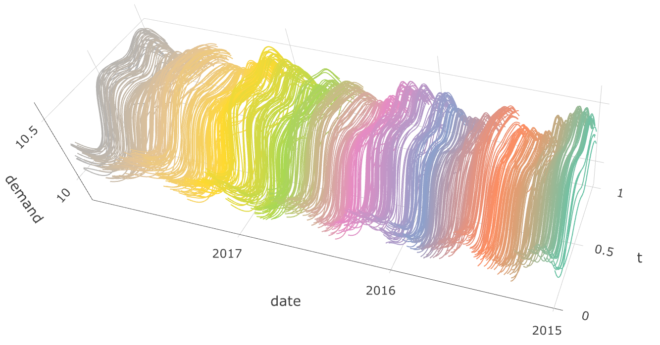
The original dataset are recorded by 10-minute intervals from 00:00–23:50 on each day, which consists of 144 observations. We consider the daily log-transformed real demand curves by smoothing and rescaling them to a continuous interval [0,1][0,1]. The plot of the smoothed functional time series is shown in Fig. 1. The stationarity test of [28] is also implemented and it turns out that the test does not reject the stationarity hypothesis at 5%5\% level during the considered period. Next, we aim to investigate the relationship between daily electricity real demand curves and future daily total demands. We explore the FLM:

Yi+1=β0+∑j=13∫01βj(t)Xi+1−j(t)dt+ϵi+1,i=3,4,…,781,Y_{i+1}=\beta_{0}+\sum_{j=1}^{3}\int_{0}^{1}\beta_{j}(t)X_{i+1-j}(t)\mathrm{d}t+\epsilon_{i+1},\,i=3,4,...,781,

where Xi+1−j​(t)X_{i+1-j}(t) stands for the daily electricity demand curve on the (i+1−j)(i+1-j)-th weekday, and Yi+1Y_{i+1} represents the daily total real demands on the (i+1)(i+1)-th weekday.

Figure 1: Functional time series plot for log-transformed electricity demands.
Refer to caption

The Legendre polynomial and FPC bases are used in this example. Firstly, we select dj,n=3d_{j,n}=3 by cumulative percentage of total variance criterion in Section 2.3, ensuring that at least 95% of the variability in the data is explained. We then set cj,n=2dj,n=6,j=1,2,3c_{j,n}=2d_{j,n}=6,~j=1,2,3. The block size is chosen as m=16m=16 by minimum volatility method in Section 2.3 for aforementioned bases, the smoothing parameter λ\lambda is selected according to the GCV criterion, yielding 8.5×10−128.5\times 10^{-12} for the Legendre polynomial bases and 4.9×10−94.9\times 10^{-9} for the FPC bases. The JSCBs are constructed in 10000 bootstrap replicates.

Figure 2: Estimated coefficient functions (black solid curve), 95%95\% JSCBs (blue dotdashed) and 95%95\% point-wise confidence bands (red dashed) with data-driven weights.

We show the plots of JSCBs and point-wise confidence bands for β1​(t),\beta_{1}(t), β2​(t)\beta_{2}(t) and β3​(t)\beta_{3}(t) in Fig. 2. Note that for each time point t∈[0,1]t\in[0,1], the coefficient βj​(t)\beta_{j}(t) is asymptotically normal. Therefore, the point-wise confidence bands can be constructed by aggregating all point-wise confidence intervals β~j​(t)±Std^​(Q^n​j​(t,λ))​qn,1−α/n\widetilde{\beta}_{j}(t)\pm\widehat{\rm Std}(\widehat{Q}_{nj}(t,\lambda))q_{n,1-\alpha}/\sqrt{n} for each single t∈[0,1]t\in[0,1], where qn,1−αq_{n,1-\alpha} is the (1−α)(1-\alpha)-th quantile of 𝒩⁡(0,1)\mathcal{N}(0,1). From Fig. 2, both β1​(t)\beta_{1}(t) and β2​(t)\beta_{2}(t) are significantly non-zero, and β3​(t)\beta_{3}(t) is insignificant under the JSCB construction for both bases. In particular, for both bases β1​(t)\beta_{1}(t) is significantly positive at the morning and evening peak times, and significantly negative at off-peak time. By contrast, β2​(t)\beta_{2}(t) is only significantly positive in the afternoon period and significantly negative in the late evening period, contributing to a slightly weaker impact on the response compared to β1​(t)\beta_{1}(t). On the other hand, while the JSCB of β3​(t)\beta_{3}(t) indicates that it is not significantly different from 0, the point-wise confidence bands for β3​(t)\beta_{3}(t) based on both bases do not fully cover the horizontal axis β3​(t)≡0\beta_{3}(t)\equiv 0, which leads to a spurious significance of β3​(t)\beta_{3}(t). These findings point to a lag 2 FLM where the electricity demands over the previous two weekdays (especially the peak time from the previous weekday) is highly correlated with the total demands of the next weekday. This also indicates that the FLM successfully captures predictive signals in demand curves when forecasting the next-day total demand. Moreover, according to the JSCB fluctuations for the coefficients β1​(t)\beta_{1}(t) and β2​(t)\beta_{2}(t), the constant coefficient hypothesis H0:βj​(t)≡CH_{0}:\beta_{j}(t)\equiv C for some finite constant CC and the linear coefficient hypothesis H0:βj​(t)=aj​t+bjH_{0}:\beta_{j}(t)=a_{j}t+b_{j} for some constants aj,bj∈ℝ,j=1,2a_{j},b_{j}\in\mathbb{R},j=1,2 are both rejected.

The evaluations of JSCBs and computations of average widths are carried out by 144 discretized data points in a curve. The average widths of SCBs for β1​(t)\beta_{1}(t) and β2​(t)\beta_{2}(t) are calculated as 4.05,3.434.05,~3.43 under Legendre polynomials and 4.77,4.024.77,~4.02 under FPC bases, respectively. For the point-wise confidence bands of β1​(t)\beta_{1}(t) and β2​(t)\beta_{2}(t), they turn out to be narrower as 2.80,2.362.80,~2.36 based on Legendre polynomials and 3.27,2.663.27,~2.66 for FPC bases. In contrast, we also implement the confidence band constructions proposed by [31] and [18]. The former method fails to detect any statistically significant coefficient functions and yields average confidence band widths of 5.90 across βj​(t),j=1,2,3\beta_{j}(t),j=1,2,3. For the latter approach, following the authors’ recommended choice of the truncation level c=⌈n2/5⌉c=\lceil n^{2/5}\rceil, all three coefficient functions βj​(t),j=1,2,3\beta_{j}(t),j=1,2,3 are identified as statistically significant. However, this comes at the cost of substantially wider confidence bands. To obtain a more appropriate truncation level for this dataset with a large sample size, we employ our cumulative percentage of total variance method to determine cc. For this case, only β1​(t)\beta_{1}(t) remains statistically significant, the resulting confidence bands remain considerably wider than those produced by our approach, with average widths of 9.82, 8.38, and 4.25 for βj​(t),j=1,2,3\beta_{j}(t),j=1,2,3, respectively.

In line with the AE’s suggestion, we extend our FLM to incorporate weather-related predictors. We consider 2015-2017 daily maximum temperatures in Spain obtained from Agencia Estatal de Meteroloíga and construct the national daily maximum temperature (TiT_{i}) as a population-weighted average across provinces using population data from Instituto Nacional de Estadística. To capture the nonlinear impact of temperature on the total demand, we introduce indicator variables Zi​1=I⁡(Ti≥r1)Z_{i1}=I(T_{i}\geq r_{1}) and Zi​2=I⁡(Ti≤r2)Z_{i2}=I(T_{i}\leq r_{2}) representing potential air conditioning and heating effects, respectively. By evaluating the linear association between the total demand and temperature variables across candidate thresholds, we select r1=31.7∘r_{1}=31.7^{\circ}C and r2=14.6∘r_{2}=14.6^{\circ}C, corresponding to temperatures at which the use of cooling and heating systems becomes more pronounced. Based on confidence intervals of the coefficients, we find that the temperature predictors are statistically significant at the 5% level. It suggests that temperature variables provides valuable information for forecasting total electricity demand.

To illustrate the prediction performance of the selected FLM in comparison with classic time series prediction methods, we apply a univariate ARIMAX model with exogenous temperature variables to predict total electricity demand on weekdays. The optimal model specification is ARIMAX(6,0,0) according to the AIC criterion.

We compare the out-of-sample forecasts for the last seven days’ total electricity demands for our FLM with temperature covariates and the above-mentioned ARIMAX(6,0,0) model. Our FLM achieves a mean squared prediction error of 0.00800.0080, an 58.75%58.75\% improvement over that of the ARIMAX model which is 0.01270.0127. These results demonstrate that functional linear regression modeling better captures high-frequency electricity demand patterns than univariate ARIMAX, leading to more accurate predictions in this dataset.

Finally, we perform an additional out-of-sample forecast to examine the prediction intervals. Specifically, we trained the model using the first 767 weekdays (with lag 2 structure and two exogenous temperature predictors) and predicted the total demand for the last 15 weekdays (three weeks) of 2017. The resulting 95% prediction intervals are in Fig. 3. Among all 15 weekdays, only two observations fall outside the 95% prediction interval. Interestingly, both correspond to Mondays. This pattern is consistent with the fact that our model is trained exclusively on weekday dynamics and does not explicitly incorporate weekend effects. Since Monday demand may depend partly on weekend consumption patterns, the reduced accuracy for those days is not unexpected.

Figure 3: The 95% Prediction intervals (blue) for the log total demand (black) over the last 15 weekdays.

5 Theoretical Results

In this section, we first model the functional time series 𝑿i​(t)\bm{X}_{i}(t) from a basis expansion and nonlinear system [62] point of view, and then investigate the multiplier bootstrap theory.

5.1 Functional Time Series Models

Based on the basis expansion (2), we aim to utilize a general time series model for {xi​j,k}k=1∞\{x_{ij,k}\}_{k=1}^{\infty} from a nonlinear system point of view. This will serve as a preliminary for our theoretical investigations.

Definition 1.

Assume that {xi​j,k}k=1∞\{x_{ij,k}\}_{k=1}^{\infty} satisfy ‖xi​j,k‖q<∞\|x_{ij,k}\|_{q}<\infty, q>9q>9, where ‖Z‖q:=𝔼​[|Z|q]1/q\|Z\|_{q}:=\mathbb{E}[|Z|^{q}]^{1/q} for a random variable ZZ. We say that {𝐗i​(t)}i∈ℤ\{\bm{X}_{i}(t)\}_{i\in\mathbb{Z}} admits a physical representation if for each fixed jj and kk, the stationary time series {xi​j,k}i=−∞∞\{x_{ij,k}\}_{i=-\infty}^{\infty} can be written as xi​j,k=Gj​k​(ℱi),x_{ij,k}=G_{jk}(\mathcal{F}_{i}), where Gj​kG_{jk} is a measurable function and ℱi=(…,ηi−1,ηi)\mathcal{F}_{i}=(...,\eta_{i-1},\eta_{i}) is the one-sided shift process with ηi\eta_{i} being i.i.d. random elements. For l≥0l\geq 0, define the ll-th physical dependence measure for the functional time series {𝐗i​(t)}\{\bm{X}_{i}(t)\} with respect to the basis {αk​(t)}k=1∞\{\alpha_{k}(t)\}_{k=1}^{\infty} and moment qq as δx​(l,q)=sup1≤j≤p,1≤k<∞‖Gj​k​(ℱi)−Gj​k​(ℱi,l)‖q,\delta_{x}(l,q)=\sup_{1\leq j\leq p,1\leq k<\infty}\|G_{jk}(\mathcal{F}_{i})-G_{jk}(\mathcal{F}_{i,l})\|_{q}, where ℱi,l=(ℱi−l−1,ηi−l∗,ηi−l+1,…,ηi)\mathcal{F}_{i,l}=(\mathcal{F}_{i-l-1},\eta_{i-l}^{\ast},\eta_{i-l+1},...,\eta_{i}) is a coupled process with ηi−l∗\eta_{i-l}^{\ast} an i.i.d. copy of ηi−l\eta_{i-l}.

Note that in the above definition, δx​(l,q)\delta_{x}(l,q) does not depend on ii. The above formulation of time series xi​j,kx_{ij,k} can be viewed as a physical system where functions Gj​kG_{jk} are the underlying data generating mechanisms and {ηi}\{\eta_{i}\} are the shocks or innovations that drive the system. Meanwhile, δx​(l,q)\delta_{x}(l,q) measures the temporal dependence of {𝑿i​(t)}\{\bm{X}_{i}(t)\} by quantifying the corresponding changes in the system’s output uniformly across all basis expansion coefficients when the shock of the system ll steps ahead is changed to an i.i.d. copy. We refer to [62] for more discussions of the physical dependence measures with examples on how to calculate them for a wide range of linear and nonlinear time series models.

Definition 1 is related to the class of functional time series formulated in [67]. The difference is that in (2) we separate the standard deviation fj​kf_{jk} from x~i​j,k\widetilde{x}_{ij,k} and the functional time series model in [67] is formulated without this extra step. Standardization of the basis expansion coefficients is needed in the fitting of the FLM (11) to avoid near singularity of the design matrix. Furthermore, Definition 1 is also related to the concept of mm-approximable functional time series introduced in [27], as both formulations utilize the concepts of Bernoulli shifts and coupling. The difference lies in our adaptation of the basis expansion, similar to that in [67], which separates the functional index tt and time index ii and hence makes it easier technically to investigate the behavior of various estimators of 𝜷⁡(t)\bm{\beta}(t) uniformly over tt. Now, we impose an assumption on the speed of decay for the dependence measures δx​(l,q)\delta_{x}(l,q).

Assumption 1.

There exists some constant τ>5\tau>5 such that for some universal constant C1>0C_{1}>0, the physical dependence measure satisfies δx​(l,q)≤C1​(l+1)−τ,l≥0.\delta_{x}(l,q)\leq C_{1}(l+1)^{-\tau},~l\geq 0.

Assumption 1 is a mild short-range dependence assumption which asserts that the temporal dependence of the functional time series 𝑿i​(t)\bm{X}_{i}(t) decays at a sufficiently fast polynomial rate. For independent functional data, the condition δx​(l,q)≤C1​(l+1)−τ\delta_{x}(l,q)\leq C_{1}(l+1)^{-\tau} is automatically satisfied as there is no temporal dependence (δx​(l,q)=0\delta_{x}(l,q)=0). In Section D of the online supplemental material, we will provide two examples on how to calculate δx​(l,q)\delta_{x}(l,q) for a class of functional MA(∞)(\infty) and functional AR(1) processes, respectively.

5.2 Validating The Multiplier Bootstrap

Adopting the nonlinear system point of view [62], we model the stationary error process {ϵi}i=1n\{\epsilon_{i}\}_{i=1}^{n} as ϵi=G⁡(ℱi)\epsilon_{i}=G(\mathcal{F}_{i}) for some measurable function GG. Observe that both 𝑿i​(t)\bm{X}_{i}(t) and ϵi\epsilon_{i} are generated by the same set of shocks {ηj}j∈ℤ\{\eta_{j}\}_{j\in\mathbb{Z}} and hence they could be statistically dependent. Further define 𝚺c​(λ)=𝔼⁡(𝑿c⊤​𝑿c)n+𝑹⁡(λ)\bm{\Sigma}_{c}(\lambda)=\frac{\mathbb{E}(\bm{X}_{c}^{\top}\bm{X}_{c})}{n}+\bm{R}(\lambda). To establish the main results, we need the following conditions:

Assumption 2.

For some non-negative integers d1d_{1} and d2d_{2} with d1≥d2d_{1}\geq d_{2}, assume that βj​(t)∈𝒞d1​([0,1])\beta_{j}(t)\in\mathcal{C}^{d_{1}}([0,1]) and Xi​j​(t)∈𝒞d2​([0,1])X_{ij}(t)\in\mathcal{C}^{d_{2}}([0,1]) a.s.. Suppose that |βj​k|≤C2​k−(d1+1)|\beta_{jk}|\leq C_{2}k^{-(d_{1}+1)}, ∀j=1,…,p\forall j=1,...,p and C2>0C_{2}>0 is some finite constant. Moreover, assume that the random coefficients ‖x~i​j,k‖2≤C3​k−(d2+1)\left\|\widetilde{x}_{ij,k}\right\|_{2}\leq C_{3}k^{-(d_{2}+1)} for i=1,…,n,j=1,…,pi=1,...,n,~j=1,...,p.

Assumption 3.

The smallest eigenvalue of 𝚺c​(λ)\bm{\Sigma}_{c}(\lambda) is greater or equal to some constant σ>0\sigma>0, which does not depend on cnc_{n} or nn.

Assumption 4.

The stationary process {ϵi}i=1n\{\epsilon_{i}\}_{i=1}^{n} satisfies ‖ϵi‖q​<∞,q>​9\|\epsilon_{i}\|_{q}<\infty,~q>9, there exist some constants C4>0C_{4}>0, and τ>5\tau>5 such that its physical dependence measure achieves δϵ​(l,q)≤C4​(l+1)−τ,l≥0\delta_{\epsilon}(l,q)\leq C_{4}(l+1)^{-\tau},~l\geq 0.

Assumption 5.

max1≤j≤c⁡𝔼​|zc​i,j|q≤Cq<∞\max_{1\leq j\leq c}\mathbb{E}|z_{ci,j}|^{q}\leq C_{q}<\infty for some Cq>0C_{q}>0.

The above conditions are mild and are needed for establishing a Gaussian approximation and comparison theory for roughness-penalized estimators. Let d≥0d\geq 0 be an integer. It is well-known that for a general 𝒞d​([0,1])\mathcal{C}^{d}([0,1]) function, the fastest decay rate for its kk-th basis expansion coefficient is O⁡(k−d−1)O(k^{-d-1}) for a wide class of basis functions [12]. For instance, the Fourier basis (for periodic functions), the weighted Chebyshev polynomials [56] and the orthogonal wavelets with degree m≥dm\geq d [41] admit the latter decay rate under some additional mild assumptions on the behavior of the function’s dd-th derivative. Hence Assumption 2 essentially requires that the basis expansion coefficients of βj​(t)\beta_{j}(t) and Xi​j​(t)X_{ij}(t) decay at the fastest rate. On the other hand, we remark that the basis expansion coefficients may decay at slower speeds for some orthonormal bases. An example is Legendre polynomials, where the coefficients decay at an O⁡(k−d−1/2)O(k^{-d-1/2}) speed [58]. For basis functions whose coefficients decay at slower rates, following the proofs of this paper it is obvious that the multiplier bootstrap method for the JSCB construction is still asymptotically valid under the corresponding restrictions on the tuning parameters. However, in this case the estimates of 𝜷⁡(t)\bm{\beta}(t) will converge at a slower speed, and the bootstrap approximation may be less accurate. For the sake of brevity, we shall stick to Assumption 2 for our theoretical investigations throughout this paper. 3 ensures positive definiteness of the design matrix in order to avoid multicollinearity. 4 is a short range dependent condition on {ϵi}i=1n\{\epsilon_{i}\}_{i=1}^{n} in accordance with 1. Finally, 5 puts some moment restrictions on the random variable zc​i,jz_{ci,j}. We refer the readers to Section E.3 for examples and discussion on these assumptions.

Let 𝑹~j\widetilde{\bm{R}}_{j} be a cj,n×cj,nc_{j,n}\times c_{j,n} matrix with its (k,l)(k,l) element R~j​(k,l)\widetilde{R}_{j}(k,l) =∫01αk′′​(t)​αl′′​(t)​𝑑t=\int_{0}^{1}\alpha_{k}^{\prime\prime}(t)\alpha_{l}^{\prime\prime}(t)\mathrm{d}t. The following additional assumptions are needed for the validation of the multiplier bootstrap.

Assumption 6.

For j=1,⋯,pj=1,\cdots,p, we assume |𝐑~j|≍cj,n2​γ|\widetilde{\bm{R}}_{j}|\asymp c_{j,n}^{2\gamma}, where γ\gamma is a positive constant depending on the basis function, and |A||A| is the spectral norm (largest singular value) of a matrix AA.

Assumption 7.

For each k≥1k\geq 1, there exists some constant ψ≥0\psi\geq 0 such that |αk​(t)|∞≤C5​kψ|\alpha_{k}(t)|_{\infty}\leq C_{5}k^{\psi} for some positive constant C5C_{5}, where |⋅|∞|\cdot|_{\infty} denotes the uniform norm of a bounded function, i.e, if f:𝒳→ℝf:\mathcal{X}\to\mathbb{R} then |f|∞=supx∈𝒳|f⁡(x)|.|f|_{\infty}=\sup_{x\in\mathcal{X}}|f(x)|. In addition, for any t1,t2∈[0,1]t_{1},~t_{2}\in[0,1] and k≥1k\geq 1, there exists a nonnegative constant ϕ\phi and some finite constant C6C_{6} such that |αk​(t1)−αk​(t2)|≤C6​kϕ​|t1−t2|.|\alpha_{k}(t_{1})-\alpha_{k}(t_{2})|\leq C_{6}k^{\phi}|t_{1}-t_{2}|.

Assumption 8.

For sufficiently large kk and j=1,⋯,pj=1,\cdots,p, |fj​k|≥C7​k−(d2+1)|f_{jk}|\geq C_{7}k^{-(d_{2}+1)}, where C7>0C_{7}>0 is a universal finite constant.

Assumption 6 is mild and can be easily checked for many frequently-used basis functions, such as the Fourier basis (γ=2)(\gamma=2) and the Legendre polynomial basis (γ=4)(\gamma=4). Meanwhile, Assumption 7 is satisfied by most frequently-used sieve bases. For instance, the pair (ψ,ϕ)=(0,1)(\psi,\phi)=(0,1) for the trigonometric polynomial series, (ψ,ϕ)=(1/2,0)(\psi,\phi)=(1/2,0) for the polynomial spline basis functions and (ψ,ϕ)=(1,5/2)(\psi,\phi)=(1,5/2) for the normalized Legendre polynomial basis. We refer to Section E.3 of the supplemental material for a detailed discussion of the above claims on Assumptions 6 and 7. Assumption 8 is frequently adopted in the FLM literature, for example [23], which imposes a lower bound on the decay rate of fj​kf_{jk}. Similar to our discussion of Assumption 2, for 𝒞d2​[0,1]\mathcal{C}^{d_{2}}[0,1] functions the fastest decay speed of their basis expansion coefficients is of the order 𝒪⁡(k−(d2+1))\mathcal{O}(k^{-(d_{2}+1)}) for a wide class of basis functions. Hence Assumption 8 is mild.

Define 𝚵c:=1n​𝔼​(∑i=1n𝒛c​i)​(∑i=1n𝒛c​i⊤)\bm{\Xi}^{c}:=\frac{1}{n}\mathbb{E}\left(\sum_{i=1}^{n}\bm{z}_{ci}\right)\left(\sum_{i=1}^{n}\bm{z}_{ci}^{\top}\right) and the Kolmogorov distance by

𝒦^​(𝑼^nb​o​o​t​s,𝒁nc):=sup𝒈n∈𝒢,x∈ℝ|ℙ⁡(supt∈[0,1]|𝑸^nb​o​o​t​s​(t,λ)|𝒈n​(t)≤x|𝒁1n)−ℙ⁡(supt∈[0,1]|𝑸nz​(t,λ)|𝒈n​(t)≤x)|.\widehat{\mathcal{K}}(\widehat{\bm{U}}_{n}^{boots},\bm{Z}_{n}^{c}):=\sup\limits_{\bm{g}_{n}\in\mathcal{G},x\in\mathbb{R}}\Big|\mathbb{P}\Big(\sup_{t\in[0,1]}\big|\widehat{\bm{Q}}_{n}^{boots}(t,\lambda)\big|_{\bm{g}_{n}(t)}\leq x\bigg|\bm{Z}_{1}^{n}\Big)-\mathbb{P}\Big(\sup_{t\in[0,1]}\big|\bm{Q}_{n}^{z}(t,\lambda)\big|_{\bm{g}_{n}(t)}\leq x\Big)\Big|.

Then we have the following theorem on the consistency of the proposed multiplier bootstrap method.

Theorem 1.

Under Assumptions 1–8, the smallest eigenvalue of 𝚵c\bm{\Xi}^{c} is bounded below by some constant b^>0\widehat{b}>0 and m=𝒪⁡(n1/3)m=\mathcal{O}(n^{1/3}). Define ℬnϵ={ω:Δn(ω):=|𝚵~c−𝚵c|F≤C8cnn−1/3hn},\mathcal{B}_{n}^{\epsilon}=\{\omega:\Delta_{n}(\omega):=|\widetilde{\bm{\Xi}}^{c}-\bm{\Xi}^{c}|_{F}\leq C_{8}c_{n}n^{-1/3}h_{n}\}, where ω\omega represents the element in the probability space, |⋅|F|\cdot|_{F} indicates Frobenius norm, hnh_{n} diverges to infinity at an arbitrarily slow rate and C8>0C_{8}>0 is a finite constant. Then ℙ⁡(ℬnϵ)=1−o⁡(1)\mathbb{P}(\mathcal{B}_{n}^{\epsilon})=1-o(1). Under the event ℬnϵ\mathcal{B}_{n}^{\epsilon}, we have

𝒦^​(𝑼^nb​o​o​t​s,𝒁nc)≤C9​χn,\widehat{\mathcal{K}}(\widehat{\bm{U}}_{n}^{boots},\bm{Z}_{n}^{c})\leq C_{9}\chi_{n},

where C9>0C_{9}>0 is some finite constant and χn→0\chi_{n}\to 0 as n,B→∞n,B\to\infty. Further suppose the conditions in Section E.1 of the supplemental material hold true, the JSCB achieves

limn→∞limB→∞ℙ⁡(βj​(t)∈CLOSE\displaystyle\lim_{n\to\infty}\lim_{B\to\infty}\mathbb{P}\Big(\beta_{j}(t)\in [β~j​(t)−q^n,1−α​g^n​j​(t)n,β~j​(t)+q^n,1−α​g^n​j​(t)n]\displaystyle\left[\widetilde{\beta}_{j}(t)-\frac{\hat{q}_{n,1-\alpha}\widehat{g}_{nj}(t)}{\sqrt{n}},\widetilde{\beta}_{j}(t)+\frac{\hat{q}_{n,1-\alpha}\widehat{g}_{nj}(t)}{\sqrt{n}}\right] (4)
for∀t∈[0,1]andj=1,…,p)=1−α.\displaystyle\text{for}~\forall t\in[0,1]~\text{and}~j=1,...,p\Big)=1-\alpha.

Theorem 3 states that under certain regularity conditions, the JSCB achieves the correct coverage probability asymptotically. In particular, χn\chi_{n} captures the rate of the bootstrap approximation to 𝑸nz​(t,λ)\bm{Q}_{n}^{z}(t,\lambda), including the Gaussian approximation error, multiplier bootstrap approximation error, and estimation error; see Section E.1 of the supplemental material for its detailed representation. The rate m=𝒪⁡(n1/3)m=\mathcal{O}(n^{1/3}) is the optimal one that balances the bias and variance of the bootstrapped covariance matrices. Since Theorem C.1 in Section C of the supplemental material and Theorem 3 above are established uniformly over all weight functions in 𝒢\mathcal{G}, the JSCB achieves asymptotically correct coverage probability without assuming that g^n​j​(t)\widehat{g}_{nj}(t) is a uniformly consistent estimator of Std​(β~j​(t))/∫01Std​(β~j​(s))​𝑑s\mbox{Std}(\widetilde{\beta}_{j}(t))/\int_{0}^{1}\mbox{Std}(\widetilde{\beta}_{j}(s))\mathrm{d}s as long as 𝒈^n​(t)∈𝒢\widehat{\bm{g}}_{n}(t)\in\mathcal{G} almost surely. Hence the multiplier bootstrap is asymptotically robust to inconsistently estimated weight functions. The price one has to pay for inconsistently estimated weight functions is that the average width of the JSCB may be inflated.

5.3 Data-Driven Basis Functions Based on Functional Principal Components

A popular data-driven orthonormal basis in functional data analysis is the FPC. Observe that FPCs have to be estimated from the data which inevitably causes estimation errors. When one employs data-driven basis functions such as the FPCs to fit model (11), the additional estimation error must be taken into account. Note that fj​k2=𝔼⁡(x~i​j,k2)f_{jk}^{2}=\mathbb{E}(\widetilde{x}_{ij,k}^{2}) are the eigenvalues of the corresponding covariance operator. Throughout this subsection, for any given jj, we assume that fj​1>fj​2>…>fj​cj,n>0f_{j1}>f_{j2}>...>f_{jc_{j,n}}>0. This assumption implies that the first cj,nc_{j,n} eigenvalues are separated, which is commonly used in the theoretical investigation for FPC-based methods. The next proposition establishes the asymptotic validity of the bootstrap for the FPC basis functions under some extra condition.

Proposition 5.1.

Under Assumptions 1–8, the multiplier bootstrap result hold true for the FPC basis functions. Further assume that

λ−2​d2+34​(γ+d2+1)>cn4​(d2+1)−d1/n\lambda^{-\frac{2d_{2}+3}{4(\gamma+d_{2}+1)}}>c_{n}^{4(d_{2}+1)-d_{1}}/\sqrt{n}{\vskip-22.76228pt} (5)

and the conditions in Section E.1 of the supplemental material are satisfied, then (4) holds for the FPC basis.

This proposition imposes an extra constraint (5) on the smoothness of 𝜷⁡(t)\bm{\beta}(t) and 𝑿i​(t)\bm{X}_{i}(t) to make the additional bias term resulting from FPC estimation negligible compared to the standard deviation term.

References

  • [1] G. Aneiros, J. Vilar, and P. Raña (2016) Short-term forecast of daily curves of electricity demand and price. Electrical Power & Energy Systems 80, pp. 96–108. Cited by: §4.
  • [2] A. Aue, L. Horváth, and D. F. Pellatt (2017) Functional generalized autoregressive conditional heteroskedasticity. Journal of Time Series Analysis 38 (1), pp. 3–21. Cited by: §1.
  • [3] A. Aue, D. D. Norinho, and S. Hörmann (2012) On the prediction of stationary functional time series. Journal of the American Statistical Association 110, pp. 378–392. External Links: http://arxiv.org/abs/1208.2892v4 Cited by: §1.
  • [4] A. Belloni, V. Chernozhukov, D. Chetverikov, and K. Kato (2015) Some new asymptotic theory for least squares series: pointwise and uniform results. Journal of Econometrics 186 (2), pp. 345–366. Cited by: §E.3.
  • [5] V. Bentkus (2003) On the dependence of the Berry–Esseen bound on dimension.. Journal of Statistical Planning and Inference 113 (2), pp. 385–402. Cited by: Appendix C, §E.4, §E.4, §1.1, §2.2.
  • [6] D. Bosq (2012) Linear processes in function spaces: theory and applications. Vol. 149, Springer Science & Business Media. Cited by: Appendix A, §1.
  • [7] T. T. Cai and M. Yuan (2012) Minimax and adaptive prediction for functional linear regression. Journal of the American Statistical Association 107 (499), pp. 1201–1216. Cited by: §1.2.
  • [8] T. T. Cai and P. Hall (2006) Prediction in functional linear regression. The Annals of Statistics 34 (5), pp. 2159–2179. Cited by: §1.2.
  • [9] H. Cardot, F. Ferraty, and P. Sarda (2003) Spline estimators for the functional linear model. Statistica Sinica 13 (3), pp. 571–591. Cited by: §1.2, §2.3.
  • [10] H. Cardot and P. Sarda (2011) Functional linear regression. In The Oxford Handbook of Functional Data Analysis, Cited by: §1.1, §1.2.
  • [11] S. Chatterjee and A. Bose (2005) Generalized bootstrap for estimating equations. The Annals of Statistics 33 (1), pp. 414–436. External Links: ISSN 0090-5364, Document Cited by: §1.2.
  • [12] X. Chen (2007) Large sample sieve estimation of semi-nonparametric models. Handbook of Econometrics 6(B), pp. 5549–5632. Cited by: §5.2.
  • [13] V. Chernozhukov, D. Chetverikov, and Kengo. Kato (2017) Central limit theorems and bootstrap in high dimensions. The Annals of Probability 45 (4), pp. 2309–2352. Cited by: §1.2.
  • [14] V. Chernozhukov, D. Chetverikov, and K. Kato (2013) Gaussian approximations and multiplier bootstrap for maxima of sums of high–dimensional random vectors. The Annals of Statistics 41 (6), pp. 2786–2819. External Links: ISSN 0090-5364, Document, MathReview Entry Cited by: §1.2.
  • [15] V. Chernozhukov, D. Chetverikov, and K. Kato (2015) Comparison and anti-concentration bounds for maxima of gaussian random vectors. Probability Theory and Related Fields 162 (1), pp. 47–70. Cited by: §E.5.
  • [16] C. Christophe, K. Alois, and P. Sarda (2009) Smoothing splines estimators for functional linear regression. The Annals of Statistics 37 (1), pp. 35–72. Cited by: §1.2.
  • [17] H. Dette, K. Kokot, and S. Volgushev (2020) Testing relevant hypotheses in functional time series via self-normalization. Journal of the Royal Statistical Society: Series B: Statistical Methodology 82, pp. 629–660. Cited by: §1.
  • [18] H. Dette and J. Tang (2024) Statistical inference for function-on-function linear regression. Bernoulli 30 (1), pp. 304–331. Cited by: §B.3, §B.3, §B.3, §1.2, §1.2, §4.
  • [19] J. Fan and R. Li (2001) Variable selection via nonconcave penalized likelihood and its oracle properties. Journal of the American Statistical Association 96 (456), pp. 1348–1360. Cited by: §E.2.
  • [20] X. Fang and Adrian. Röllin (2015) Rates of convergence for multivariate normal approximation with applications to dense graphs and doubly indexed permutation statistics. Bernoulli 21 (4), pp. 2157–2189. Cited by: Appendix C, Lemma E.1.
  • [21] X. Fang (2016) A multivariate CLT for bounded decomposable random vectors with the best known rate. Journal of Theoretical Probability 29 (4), pp. 1510–1523. Cited by: Appendix C, §E.4, §E.4, §E.4, §E.4, Lemma E.2, §1.1, §2.2.
  • [22] E. García-Portugués, W. González-Manteiga, and M. Febrero-Bande (2014) A goodness-of-fit test for the functional linear model with scalar response. Journal of Computational and Graphical Statistics 23 (3), pp. 761–778. Cited by: §1.2.
  • [23] P. Hall and J. L. Horowitz (2007) Methodology and convergence rates for functional linear regression. The Annals of Statistics 35 (1), pp. 70–91. Cited by: §E.6, §5.2.
  • [24] P. Hall, H. Müller, and J. Wang (2006) Properties of principal component methods for functional and longitudinal data analysis. The Annals of Statistics 34 (3), pp. 1493–1517. Cited by: Appendix A.
  • [25] N. Hilgert, A. Mas, and N. Verzelen (2013) Minimax adaptive tests for the functional linear model. The Annals of Statistics 41 (2), pp. 838–869. Cited by: §1.2.
  • [26] S. Hörmann and Ł. Kidziński (2015) A note on estimation in Hilbertian linear models. Scandinavian Journal of Statistics 42 (1), pp. 43–62. Cited by: §1.2.
  • [27] S. Hörmann and P. Kokoszka (2010) Weakly dependent functional data. The Annals of Statistics 38 (3), pp. 1845–1884. Cited by: §1.2, §1, §5.1.
  • [28] L. Horváth, P. Kokoszka, and G. Rice (2014) Testing stationarity of functional time series. Journal of Econometrics 179 (1), pp. 66–82. Cited by: §4.
  • [29] L. Horváth and P. Kokoszka (2012) A test of significance in functional quadratic regression. In Inference for Functional Data with Applications, pp. 225–232. Cited by: §1.2.
  • [30] L. Horváth and P. Kokoszka (2012) Inference for functional data with applications. Springer Science & Business Media. Cited by: §1.
  • [31] M. Imaizumi and K. Kato (2019) A simple method to construct confidence bands in functional linear regression. Statistica Sinica 29 (4), pp. 2055–2081. Cited by: §B.3, §B.3, §B.3, §B.3, §1.2, §4.
  • [32] G. M. James, J. Wang, and J. Zhu (2009) Functional linear regression that’s interpretable. The Annals of Statistics 37 (5A), pp. 2083–2108. Cited by: §1.2.
  • [33] D. Kong, A. Staicu, and A. Maity (2016) Classical testing in functional linear models. Journal of Nonparametric Statistics 28 (4), pp. 813–838. Cited by: §1.2.
  • [34] S. N. Lahiri (2003) Resampling methods for dependent data. New York: Springer. Cited by: §2.2.
  • [35] J. Lei (2014) Adaptive global testing for functional linear models. Journal of the American Statistical Association 109 (506), pp. 624–634. Cited by: §1.2.
  • [36] Y. Li and T. Hsing (2007) On rates of convergence in functional linear regression. Journal of Multivariate Analysis 98 (9), pp. 1782–1804. Cited by: §E.2, §1.2.
  • [37] Y. Li and T. Hsing (2010) Uniform convergence rates for nonparametric regression and principal component analysis in functional/longitudinal data. The Annals of Statistics 38 (6), pp. 3321–3351. Cited by: §E.6.
  • [38] W. Liu and Z. Lin (2009) Strong approximation for a class of stationary processes. Stochastic Processes and their Applications 119 (1), pp. 249–280. Cited by: §E.4.
  • [39] S. Ma and M. R. Kosorok (2005) Robust semiparametric M-estimation and the weighted bootstrap. Journal of Multivariate Analysis 96, pp. 190–217. External Links: ISSN 0047-259X, Document Cited by: §1.2.
  • [40] M. W. McLean, G. Hooker, and D. Ruppert (2015) Restricted likelihood ratio tests for linearity in scalar-on-function regression. Statistics and Computing 25 (5), pp. 997–1008. Cited by: §1.2.
  • [41] Y. Meyer (1992) Ondelettes et operateurs i: ondelettes. Hermann, Paris. Cited by: §5.2.
  • [42] J. S. Morris (2015) Functional regression. Annual Review of Statistics and Its Application 2, pp. 321–359. Cited by: §1.2.
  • [43] W. K. Newey and K. D. West (1987) A simple, positive semi-definite, heteroskedasticity and autocorrelation consistent covariance matrix. Econometrica 55 (3), pp. 703–708. External Links: ISSN 00129682, 14680262, Link Cited by: §2.2.
  • [44] W. K. Newey (1997) Convergence rates and asymptotic normality for series estimators. Journal of Econometrics 79 (1), pp. 147–168. External Links: ISSN 0304-4076, Document Cited by: §E.3.
  • [45] V. M. Panaretos and S. Tavakoli (2013) Fourier analysis of stationary time series in function space. The Annals of Statistics 41 (2), pp. 568–603. Cited by: §1.
  • [46] Efstathios. Paparoditis (2018) Sieve bootstrap for functional time series. The Annals of Statistics 46 (6B), pp. 3510–3538. Cited by: §1.
  • [47] D.N. Politis, J.P. Romano, and M. Wolf (1999) Subsampling. Springer Science & Business Media. Cited by: §2.3.
  • [48] J.O. Ramsay and B.W. Silverman (2005) Functional data analysis. 2nd edition, New York: Springer. Cited by: §2.1.
  • [49] P. T. Reiss, J. Goldsmith, H. L. Shang, and R. T. Ogden (2017) Methods for scalar-on-function regression. International Statistical Review 85 (2), pp. 228–249. Cited by: Appendix A, §1.2.
  • [50] P. T. Reiss and R. T. Ogden (2007) Functional principal component regression and functional partial least squares. Journal of the American Statistical Association 102 (479), pp. 984–996. External Links: ISSN 0162-1459, Document Cited by: §2.3.
  • [51] B. A. Schmitt (1992) Perturbation bounds for matrix square roots and pythagorean sums. Linear Algebra and its Applications 174, pp. 215–227. Cited by: §E.5.
  • [52] H. L. Shang (2014) A survey of functional principal component analysis. AStA Advances in Statistical Analysis 98 (2), pp. 121–142. Cited by: §2.1.
  • [53] Z. Shang and G. Cheng (2015) Nonparametric inference in generalized functional linear models. The Annals of Statistics 43 (3), pp. 1742–1773. External Links: ISSN 0090-5364, Document Cited by: §E.2, §1.2, §1.2.
  • [54] V. Spokoiny and M. Zhilova (2015) Bootstrap confidence sets under model misspecification. The Annals of Statistics 43 (6), pp. 2653–2675. External Links: ISSN 0090-5364, Document Cited by: §1.2.
  • [55] Y. Su, C. Di, and L. Hsu (2017) Hypothesis testing in functional linear models. Biometrics 73 (2), pp. 551–561. Cited by: §1.2.
  • [56] L. N. Trefethen (2008) Is Gauss quadrature better than Clenshaw–Curtis?. SIAM Review 50 (1), pp. 67–87. Cited by: §5.2.
  • [57] J. A. Tropp (2012) User-friendly tail bounds for sums of random matrices. Foundations of computational mathematics 12 (4), pp. 389–434. Cited by: §E.7.
  • [58] H. Wang and S. Xiang (2012) On the convergence rates of Legendre approximation. Mathematics of Computation 81 (278), pp. 861–877. Cited by: §5.2.
  • [59] J. Wang, J. Chiou, and H. Müller (2016) Functional data analysis. Annual Review of Statistics and Its Application 3, pp. 257–295. Cited by: §1.2.
  • [60] C. J. Wu (1986) Jackknife, bootstrap and other resampling methods in regression analysis. The Annals of Statistics 14 (4), pp. 1261–1295. Cited by: §2.2.
  • [61] W. B. Wu and Z. Zhao (2007) Inference of trends in time series. Journal of the Royal Statistical Society: Series B: Statistical Methodology 69 (3), pp. 391–410. Cited by: Appendix A.
  • [62] W. B. Wu (2005) Nonlinear system theory: another look at dependence. Proceedings of the National Academy of Sciences 102 (40), pp. 14150–14154. Cited by: §E.3, §E.6, §E.7, §5.1, §5.2, §5.
  • [63] F. Yao, H. Müller, and J. Wang (2005) Functional data analysis for sparse longitudinal data. Journal of the American Statistical Association 100 (470), pp. 577–590. Cited by: Appendix A.
  • [64] M. Yuan and T. T. Cai (2010) A reproducing kernel hilbert space approach to functional linear regression. The Annals of Statistics 38 (6), pp. 3412–3444. Cited by: §1.2.
  • [65] J. Zhang and J. Chen (2007) Statistical inferences for functional data. The Annals of Statistics 35 (3), pp. 1052–1079. Cited by: Appendix A.
  • [66] X. Zhang and G. Cheng (2018) Gaussian approximation for high dimensional vector under physical dependence. Bernoulli 24 (4A), pp. 2640–2675. Cited by: §E.7.
  • [67] Z. Zhou and H. Dette (2023) Statistical inference for high-dimensional panel functional time series. Journal of the Royal Statistical Society Series B: Statistical Methodology 85 (2), pp. 523–549. External Links: ISSN 1369-7412, Document Cited by: §1.2, §5.1.
  • [68] Z. Zhou (2013) Heteroscedasticity and autocorrelation robust structural change detection. Journal of the American Statistical Association 108 (502), pp. 726–740. External Links: Document Cited by: §E.7, §E.7.

Supplementary Material of ”Simultaneous Inference for Time Series Functional Linear Regression”

Appendix A Discussion on the Main Article

We now discuss some issues related to the practical implementation of the regression as well as possible extensions. Firstly, the predictors 𝑿i​(t)\bm{X}_{i}(t) are typically only discretely observed with noises. Hence, pre-smoothing is required to transfer the discretely observed predictors into continuous curves which inevitably produces some smoothing errors. In this article, for the purposes of brevity and to keep the discussion focused, we assume that the smooth curves of 𝑿i​(t)\bm{X}_{i}(t) are observed. It can be seen from the proofs that the results of the paper hold under the densely observed functional data scenario as long as the smoothing error achieves an order Oℙ​(log⁡n/n)O_{\mathbb{P}}(\log n/\sqrt{n}) uniformly. Smoothing for time series or densely observed functional data has been intensively investigated in the literature; see for instance [24], [65] and [61], among many others. Though the aforementioned references are not exactly intended for functional time series, their results can be extended to the functional time series setting, which we will pursue in a separate future work. On the other hand, we do not expect that our theory and methodology will directly carry over to the sparsely observed functional data setting [63], and the corresponding investigations are beyond the scope of the current paper.

Secondly, we note that the choice of basis functions is a non-trivial task in practice. In the literature, there are several discussions with respect to the choice of basis functions, or methods for the functional linear regression models in general. See for instance Section 6.1 in [49] and the references therein. Here we shall add some additional notes. For functional time series whose observation curves are clearly periodic, such as the yearly temperature curves, the Fourier basis is a natural choice. Similar choices can be made based on prior knowledge of the shapes of the observation curves in various scenarios. Our limited simulation studies and data analysis in Sections 3 and 4 of the main article suggested many popular classes of basis functions produce similar estimates of the regression curves and comparable inference results, which demonstrates a certain level of robustness towards the basis choices.

Finally, in some real data applications the response time series may be function-valued as well. One prominent example is functional auto-regression [6]. We hope that our multiplier bootstrap methodology as well as the underlying Gaussian approximation and comparison results will shed light on the simultaneous inference problem for FLM with functional responses. We will investigate this direction in a future research endeavor.

Appendix B Additional Simulation Results

In this section we would like to conduct some additional simulation studies that complement those in Section 3 of the main paper. The significance levels are set at α=0.05\alpha=0.05 and 0.10.1. We choose the sample size as n=400,800n=400,800 and the bootstrap replications B=1000B=1000 based on 1000 simulation runs throughout this section.

B.1 Simulation Studies for an FAR(1) Model

To measure the effects of temporal dependence, we also conduct a simulation study for an FAR(1) model. First, we consider β⁡(t)=∑k=1∞βk​αk​(t),Xi​(t)=∑k=1∞x~i​k​αk​(t)\beta(t)=\sum_{k=1}^{\infty}\beta_{k}\alpha_{k}(t),X_{i}(t)=\sum_{k=1}^{\infty}\widetilde{x}_{ik}\alpha_{k}(t) and denote 𝒙~i=(x~i​1,x~i​2,…)⊤\widetilde{\bm{x}}_{i}=(\widetilde{x}_{i1},\widetilde{x}_{i2},\ldots)^{\top}. The autoregressive model can be constructed as
∙\bullet 𝒙~i=ϕ2​𝑫​𝒙~i−1+𝜼i\widetilde{\bm{x}}_{i}=\phi_{2}\bm{D}\widetilde{\bm{x}}_{i-1}+\bm{\eta}_{i} with ϕ2∈[0,0.723)\phi_{2}\in[0,0.723), and we choose the AR coefficient ϕ2=0,0.2\phi_{2}=0,0.2 or 0.50.5 to represent weak to moderately strong dependencies. The entries {ηi​k}k=1∞\{\eta_{ik}\}_{k=1}^{\infty} of 𝜼i\bm{\eta}_{i} are chosen as independent 𝒩⁡(0,e−(k−1))\mathcal{N}(0,{\rm e}^{-(k-1)}) random variables.

Furthermore, the generating mechanism for β⁡(t)\beta(t) and error process can be given by
∙\bullet β1=0.8,β2=0.5,β3=−0.3\beta_{1}=0.8,~\beta_{2}=0.5,~\beta_{3}=-0.3 and βk=e−k\beta_{k}=e^{-k} for k≥4k\geq 4. {ϵi}i=1n\{\epsilon_{i}\}_{i=1}^{n} are independent of Xi​(t)X_{i}(t). Let {ϵi}i=1n\{\epsilon_{i}\}_{i=1}^{n} follow an AR(1) process ϵi=0.2​ϵi−1+ei\epsilon_{i}=0.2\epsilon_{i-1}+e_{i} where eie_{i} is i.i.d. standard normally distributed.

Table 2: Simulated coverage probabilities with average JSCB widths in parentheses.
n=400n=400
1−α=0.951-\alpha=0.95 1−α=0.901-\alpha=0.90
g^n​j\widehat{g}_{nj} Basis ϕ2=0\phi_{2}=0 0.20.2 0.50.5 ϕ2=0\phi_{2}=0 0.20.2 0.50.5
1 Fou. 0.945(1.77) 0.944(1.79) 0.935(1.72) 0.898(1.55) 0.883(1.56) 0.884(1.51)
Leg. 0.942(3.10) 0.947(3.16) 0.940(3.05) 0.901(2.67) 0.888(2.72) 0.877(2.64)
FPC 0.939(1.91) 0.941(1.91) 0.947(1.90) 0.893(1.67) 0.889(1.66) 0.892(1.66)
Std{\rm Std} Fou. 0.938(1.47) 0.932(1.47) 0.923(1.43) 0.884(1.32) 0.876(1.32) 0.864(1.29)
Leg. 0.934(1.50) 0.923(1.53) 0.922(1.56) 0.883(1.35) 0.870(1.37) 0.860(1.40)
FPC 0.938(1.58) 0.927(1.57) 0.923(1.56) 0.871(1.41) 0.869(1.41) 0.851(1.40)
n=800n=800
1−α=0.951-\alpha=0.95 1−α=0.901-\alpha=0.90
g^n​j\widehat{g}_{nj} Basis ϕ2=0\phi_{2}=0 0.20.2 0.50.5 ϕ2=0\phi_{2}=0 0.20.2 0.50.5
1 Fou. 0.960(1.25) 0.944(1.27) 0.940(1.23) 0.903(1.10) 0.896(1.11) 0.891(1.08)
Leg. 0.959(2.12) 0.946(2.12) 0.940(2.14) 0.908(1.83) 0.894(1.83) 0.888(1.85)
FPC 0.952(1.28) 0.952(1.30) 0.955(1.26) 0.909(1.12) 0.893(1.14) 0.914(1.10)
Std{\rm Std} Fou. 0.947(1.04) 0.940(1.06) 0.930(1.02) 0.890(0.93) 0.878(0.95) 0.871(0.91)
Leg. 0.940(1.02) 0.944(1.04) 0.938(1.04) 0.895(0.91) 0.886(0.93) 0.886(0.93)
FPC 0.942(1.06) 0.939(1.08) 0.934(1.04) 0.889(0.95) 0.882(0.97) 0.887(0.93)

The simulated coverage probabilities and average widths of the joint simultaneous confidence bands (JSCB) with two types of weight functions are reported in Table 2. It is obvious to find that when n=400n=400 and the data-adaptive weights are used, the coverage probabilities are reasonably close to the nominal levels for most cases under weaker dependence (ϕ2=0,0.2\phi_{2}=0,0.2). However, under stronger dependence the performances of the three bases weaken slightly when n=400n=400. The decrease in estimation accuracy and coverage probability in finite samples under stronger temporal dependence is well-known in time series analysis. This decrease seems to be universal across various inferential tools (such as subsampling, block bootstrap, multiplier bootstrap, and self-normalization) though some methods may be less sensitive to stronger dependence. One explanation is that the variances of the estimators tend to be higher under stronger dependence, which leads to less accurate estimators. This reduced accuracy then results in deteriorated coverage probabilities in small to moderately large samples.

B.2 Simulation Studies for Brownian Motions

We consider an additional simulation experiment where the functional predictor Xi​(t)X_{i}(t) is a Brownian motion process. We use three types of basis functions, Fourier bases, shifted Jacobi polynomial bases and functional principal components (FPC). First, we list the following approximation representations for the generation of Brownian motions Xi​(t)X_{i}(t) based on two kinds of basis functions:
∙\bullet Fourier bases:

Xi​(t)=Z0​t+∑k=1∞2​Zkπ​k​sin⁡(k​π​t),X_{i}(t)=Z_{0}t+\sum_{k=1}^{\infty}\frac{\sqrt{2}Z_{k}}{\pi k}\sin(k\pi t),

where Zk,k≥0Z_{k},k\geq 0 are independent and identically distributed (i.i.d.) 𝒩⁡(0,1)\mathcal{N}(0,1) random variables.
∙\bullet Shifted Jacobi polynomial bases:

Xi​(t)=Z0​t+∑k=1∞Zk​ϕk​(t),X_{i}(t)=Z_{0}t+\sum_{k=1}^{\infty}Z_{k}\phi_{k}(t),

where Z0∼𝒩⁡(0,1),Zk∼𝒩⁡(0,k−1​(k+1)−1)Z_{0}\sim\mathcal{N}(0,1),Z_{k}\sim\mathcal{N}(0,k^{-1}(k+1)^{-1}) for k≥1k\geq 1 and all Zk,k≥0Z_{k},k\geq 0 are independent. {ϕk​(t)}k≥1\{\phi_{k}(t)\}_{k\geq 1} are orthogonal basis functions constructed by Jacobi polynomial bases as

ϕk​(t)=k​(k+1)​(2​k+1)k​Pk+1(−1,−1)​(2​t−1),t∈[0,1]\phi_{k}(t)=\frac{\sqrt{k(k+1)(2k+1)}}{k}P_{k+1}^{(-1,-1)}(2t-1),~t\in[0,1]

where Pk+1(−1,−1)​(⋅)P_{k+1}^{(-1,-1)}(\cdot) is the (−1,−1)(-1,-1)-Jacobi polynomial defined by

Pk+1(−1,−1)​(t)=k4​k+2​[Pk+1​(t)−Pk−1​(t)],t∈[−1,1]P_{k+1}^{(-1,-1)}(t)=\frac{k}{4k+2}[P_{k+1}(t)-P_{k-1}(t)],~t\in[-1,1]

with the original Legendre polynomial Pk​(t)P_{k}(t) defined in Example 5 of Section E.3.

Now, restate the basis expansion β⁡(t)=∑k=1∞βk​αk​(t)\beta(t)=\sum_{k=1}^{\infty}\beta_{k}\alpha_{k}(t) when p=1p=1. We consider the following parameter configurations:
∙\bullet β1=0.8,β2=0.5,β3=−0.3\beta_{1}=0.8,\beta_{2}=0.5,\beta_{3}=-0.3 and βk=e−k\beta_{k}={\rm e}^{-k} for k≥4k\geq 4.
∙\bullet Case (a): (Xi​(t),Yi)(X_{i}(t),Y_{i}) are i.i.d. and the error process {ϵi}i=1n\{\epsilon_{i}\}_{i=1}^{n} are i.i.d. with 𝒩⁡(0,0.25)\mathcal{N}(0,0.25).
∙\bullet Case (b): Xi​(t)X_{i}(t) are i.i.d. across ii and {ϵi}i=1n\{\epsilon_{i}\}_{i=1}^{n} follow an AR(1) process ϵi=0.2​ϵi−1+ei\epsilon_{i}=0.2\epsilon_{i-1}+e_{i}, where eie_{i} is i.i.d. with 𝒩⁡(0,0.25)\mathcal{N}(0,0.25). Furthermore, {ϵi}i=1n\{\epsilon_{i}\}_{i=1}^{n} are independent of {Xi​(t)}i=1n\{X_{i}(t)\}_{i=1}^{n}.

Similar to the simulation studies in Section 3 of the main paper, the evaluations of the JSCB and computations of the average widths are carried out by discretizing the unit interval [0,1][0,1] into 100100 equally spaced grids. Table 3 shows simulated coverage probabilities and average JSCB widths with three types of basis functions based on both constant and data-driven weight functions. From that, one can observe that most of the results, especially for n=800n=800, are close to the nominal levels. Specifically, the average widths of JSCB for g^n​j​(t)=Std^​(Q^n​jb​o​o​t​s​(t,λ))/∫01Std^​(Q^n​jb​o​o​t​s​(s,λ))​𝑑s\widehat{g}_{nj}(t)=\widehat{\rm Std}(\widehat{Q}_{nj}^{boots}(t,\lambda))\big/\int_{0}^{1}\widehat{\rm Std}(\widehat{Q}_{nj}^{boots}(s,\lambda))\mathrm{d}s are narrower than those for gn​j​(t)≡1g_{nj}(t)\equiv 1. In summary, we claim that our methodology can be applied to the scenario where the functional data is continuous but non-differentiable everywhere, such as Brownian motion.

Table 3: Simulated coverage probabilities for the Brownian motion case.
Case (a) 1−α=0.951-\alpha=0.95 1−α=0.901-\alpha=0.90
g^n​j\widehat{g}_{nj} Basis n=400n=400 n=800n=800 n=400n=400 n=800n=800
1 Fourier 0.947(0.99) 0.946(0.67) 0.898(0.87) 0.889(0.59)
Jacobi 0.934(1.66) 0.934(1.27) 0.882(1.49) 0.886(1.14)
FPC 0.947(0.97) 0.946(0.66) 0.895(0.85) 0.889(0.58)
Std Fourier 0.934(0.86) 0.935(0.58) 0.870(0.78) 0.879(0.52)
Jacobi 0.929(1.60) 0.936(1.22) 0.880(1.45) 0.872(1.11)
FPC 0.934(0.85) 0.934(0.57) 0.872(0.76) 0.879(0.52)
Case (b) 1−α=0.951-\alpha=0.95 1−α=0.901-\alpha=0.90
g^n​j\widehat{g}_{nj} Basis n=400n=400 n=800n=800 n=400n=400 n=800n=800
1 Fourier 0.934(0.99) 0.937(0.69) 0.877(0.87) 0.889(0.60)
Jacobi 0.936(1.70) 0.942(1.30) 0.886(1.52) 0.880(1.16)
FPC 0.935(0.97) 0.937(0.68) 0.890(0.85) 0.890(0.60)
Std Fourier 0.937(0.86) 0.938(0.59) 0.876(0.77) 0.889(0.53)
Jacobi 0.930(1.62) 0.942(1.24) 0.874(1.47) 0.881(1.13)
FPC 0.935(0.84) 0.939(0.59) 0.876(0.76) 0.888(0.53)

B.3 Numerical Experiments Comparing with Other Methods

In this subsection, we conduct another simulation study, comparing our JSCB construction with the conservative confidence bands proposed by [31] and the confidence bands construction investigated by [18]. Since the methodologies of the latter two papers are limited to i.i.d. data, we will perform three distinct sets of comparison experiment with p=1p=1, including i.i.d. scenario, weak temporal dependent and moderately strong dependent cases. Here, recall the basis expansions as β⁡(t)=∑k=1∞βk​αk​(t),Xi​(t)=∑k=1∞x~i​k​αk​(t)\beta(t)=\sum_{k=1}^{\infty}\beta_{k}\alpha_{k}(t),X_{i}(t)=\sum_{k=1}^{\infty}\widetilde{x}_{ik}\alpha_{k}(t). Consider
∙\bullet β1=0.8,β2=0.5,β3=−0.3\beta_{1}=0.8,\beta_{2}=0.5,\beta_{3}=-0.3 and βk=e−k\beta_{k}={\rm e}^{-k} for k≥4k\geq 4.
∙\bullet x~i​k=k−1​Uk\widetilde{x}_{ik}=k^{-1}U_{k} where {Uk}k=1∞\{U_{k}\}_{k=1}^{\infty} i.i.d. follow the Uniform distribution as Unif⁡(−3,3){\rm Unif}(-\sqrt{3},\sqrt{3}).

Now, we investigate the following cases:
∙\bullet Case (c): Consider the above data generation processes for β⁡(t)\beta(t) and Xi​(t)X_{i}(t), and the error term ϵi\epsilon_{i} is i.i.d. 𝒩⁡(0,1)\mathcal{N}(0,1).
∙\bullet Case (d): The above data generation processes for β⁡(t)\beta(t) and Xi​(t)X_{i}(t) are considered, the error process {ϵi}i=1n\{\epsilon_{i}\}_{i=1}^{n} follows an AR(1) model ϵi=0.2​ϵi−1+ei\epsilon_{i}=0.2\epsilon_{i-1}+e_{i} where eie_{i} is i.i.d. 𝒩⁡(0,1)\mathcal{N}(0,1).
∙\bullet Case (e): The generation process for β⁡(t)\beta(t) retains the same of that in Case (d), Xi​(t)X_{i}(t) follows the FAR(1) model in Section 4 of the main paper where the coefficient matrix 𝑫\bm{D} is diagonal with all diagonal elements being 1 to make sure the true FPCs of Xi​(t)X_{i}(t) are {αk​(t)}k=1∞\{\alpha_{k}(t)\}_{k=1}^{\infty} and the autoregressive coefficient ϕ=0.5\phi=0.5. The error process follows the same AR(1) model as described in Case (d).

Table 4: Simulated coverage probabilities and average widths for MCP, MCP∗ and JSCB.
Case (c) τ1=0.05\tau_{1}=0.05 τ1=0.10\tau_{1}=0.10
Method Cutoff level/Weight n=400n=400 n=800n=800 n=400n=400 n=800n=800
MCP max⁡{m^n,2}\max\{\widehat{m}_{n},2\} 0.985(1.94) 0.947(1.51) 0.926(1.68) 0.862(1.32)
m^n+1\widehat{m}_{n}+1 0.999(2.72) 1(2.04) 0.999(2.40) 1(1.80)
MCP∗ max⁡{m^n,2}\max\{\widehat{m}_{n},2\} 0.917(1.94) 0.874(1.51) 0.795(1.69) 0.820(1.32)
m^n+1\widehat{m}_{n}+1 0.995(2.72) 1(2.04) 0.987(2.40) 1(1.80)
JSCB g^n​1=Std\widehat{g}_{n1}={\rm Std} 0.940(2.63) 0.941(1.88) 0.887(2.38) 0.893(1.70)
Case (d) τ1=0.05\tau_{1}=0.05 τ1=0.10\tau_{1}=0.10
Method Cutoff level/Weight n=400n=400 n=800n=800 n=400n=400 n=800n=800
MCP max⁡{m^n,2}\max\{\widehat{m}_{n},2\} 0.985(1.97) 0.936(1.53) 0.935(1.62) 0.844(1.34)
m^n+1\widehat{m}_{n}+1 1(2.75) 1(2.11) 1(2.42) 1(1.86)
MCP∗ max⁡{m^n,2}\max\{\widehat{m}_{n},2\} 0.928(1.87) 0.858(1.53) 0.807(1.62) 0.785(1.34)
m^n+1\widehat{m}_{n}+1 0.995(2.75) 0.999(2.11) 0.990(2.42) 0.993(1.86)
JSCB g^n​1=Std\widehat{g}_{n1}={\rm Std} 0.926(2.67) 0.944(1.92) 0.871(2.42) 0.887(1.74)
Case (e) τ1=0.05\tau_{1}=0.05 τ1=0.10\tau_{1}=0.10
Method Cutoff level/Weight n=400n=400 n=800n=800 n=400n=400 n=800n=800
MCP max⁡{m^n,2}\max\{\widehat{m}_{n},2\} 0.896(1.79) 0.888(1.34) 0.784(1.56) 0.884(1.16)
m^n+1\widehat{m}_{n}+1 1(2.90) 1(2.41) 1(2.52) 0.999(2.09)
MCP∗ max⁡{m^n,2}\max\{\widehat{m}_{n},2\} 0.804(1.79) 0.885(1.34) 0.712(1.56) 0.867(1.16)
m^n+1\widehat{m}_{n}+1 0.999(2.90) 0.999(2.41) 0.999(2.52) 0.996(2.09)
JSCB g^n​1=Std\widehat{g}_{n1}={\rm Std} 0.930(1.53) 0.936(1.03) 0.862(1.37) 0.879(0.92)

In the simulation experiment, we focus on Fourier basis functions αk​(t)={1,2​cos⁡(π​t),2​cos⁡(2​π​t),⋯}\alpha_{k}(t)=\{1,\sqrt{2}\cos(\pi t),\\ \sqrt{2}\cos(2\pi t),\cdots\} and examine the coverage probabilities of confidence bands for sample sizes n=400,800n=400,800 with 10001000 replicates. For the conservative confidence bands construction in [31], we choose the significance levels τ1=0.05,0.1\tau_{1}=0.05,0.1, the other level τ2=0.1\tau_{2}=0.1 and preserve two kinds of choices for the cutoff level (i.e. truncation number used in the PCA-based estimation) mnm_{n}, denoted by max⁡{m^n,2}\max\{\widehat{m}_{n},2\} and m^n+1\widehat{m}_{n}+1. To provide further clarity, we evaluate the confidence bands of our method in comparison with methods in [31] using

JSCB\displaystyle{\rm JSCB} =ℙ(β(t)∈[β~(t)−g^n​1(t)q^n,1−τ1/n,β~(t)+g^n​1(t)q^n,1−τ1/n],∀t∈[0,1]),\displaystyle=\mathbb{P}\big(\beta(t)\in[\widetilde{\beta}(t)-\widehat{g}_{n1}(t)\hat{q}_{n,1-\tau_{1}}/\sqrt{n},\widetilde{\beta}(t)+\widehat{g}_{n1}(t)\hat{q}_{n,1-\tau_{1}}/\sqrt{n}],\forall t\in[0,1]\big),
MCP\displaystyle{\rm MCP} =ℙ⁡(μ⁡({t∈[0,1],β⁡(t)∉𝒞^​(t)})≤τ2),\displaystyle=\mathbb{P}\big(\mu\big(\{t\in[0,1],\beta(t)\notin\widehat{\mathcal{C}}(t)\}\big)\leq\tau_{2}\big),
MCP∗\displaystyle{\rm MCP}^{\ast} =ℙ(β(t)∈𝒞^(t),∀t∈[0,1]),\displaystyle=\mathbb{P}\big(\beta(t)\in\widehat{\mathcal{C}}(t),\forall t\in[0,1]\big),

where g^n​1​(t)=Std^​(Q^n​1​(t,λ))/∫01Std^​(Q^n​1​(s,λ))​𝑑s\widehat{g}_{n1}(t)=\widehat{\rm Std}(\widehat{Q}_{n1}(t,\lambda))\big/\int_{0}^{1}\widehat{\rm Std}(\widehat{Q}_{n1}(s,\lambda))\mathrm{d}s is considered in the JSCB construction. The confidence bands in MCP construction are specified as

𝒞^​(t)=[β~​(t)−σ^​c^n,1−τ1n​1τ2​μ​([0,1]),β~​(t)+σ^​c^n,1−τ1n​1τ2​μ​([0,1])]\widehat{\mathcal{C}}(t)=\left[\widetilde{\beta}(t)-\frac{\widehat{\sigma}\widehat{c}_{n,1-\tau_{1}}}{\sqrt{n}}\sqrt{\frac{1}{\tau_{2}\mu([0,1])}},\widetilde{\beta}(t)+\frac{\widehat{\sigma}\widehat{c}_{n,1-\tau_{1}}}{\sqrt{n}}\sqrt{\frac{1}{\tau_{2}\mu([0,1])}}\right]

with c^n,1−τ1\widehat{c}_{n,1-\tau_{1}} representing the simulated conditional (1−τ1)(1-\tau_{1})-quantile of the corresponding statistic given functional data {X1​(t),…,Xn​(t)}\{X_{1}(t),...,X_{n}(t)\}, σ^=n−1​∑i=1n[Yi−∑k=1m^nx^i​k​β^k]2\widehat{\sigma}=\sqrt{n^{-1}\sum_{i=1}^{n}[Y_{i}-\sum_{k=1}^{\widehat{m}_{n}}\widehat{x}_{ik}\widehat{\beta}_{k}]^{2}} where x^i​k\widehat{x}_{ik} is the estimated FPC score and β^k\widehat{\beta}_{k} is the estimated coefficient of βk\beta_{k}. The notation μ\mu in the equation of MCP denotes the Lebesgue measure.

The simulated coverage probabilities and average widths for JSCB, MCP and MCP∗ are shown in Table 4. For the MCP method proposed in [31], when the cutoff level is chosen as max⁡{m^n,2}\max\{\widehat{m}_{n},2\}, the coverage probabilities for Cases (c) and (d) exceed the nominal levels for n=400n=400, while most coverage probabilities are below the nominal level for n=800n=800. Furthermore, when the cutoff level is specified as max⁡{m^n,2}\max\{\widehat{m}_{n},2\}, most of the coverage probabilities under MCP turn out to decrease as the sample size increases, which implies possible instability in simultaneous coverage of this confidence band construction. We note that the observed instability possibly stems from the fact that the MCP method aims at covering the slope function at “most” of the points t∈[0,1]t\in[0,1] with a prespecified probability, but is not designed for simultaneous coverage. On the other hand, the simulated coverage probabilities for MCP based on the cutoff level m^n+1\widehat{m}_{n}+1 appear to be close to 1 in Cases (c)–(e), at the cost of substantially wider confidence bands.

Note that we also include MCP∗ construction with a stringent requirement. Instead of allowing a small proportion (τ2\tau_{2}) of the set of points not covered by the confidence bands in MCP construction, MCP∗ method evaluates the coverage probabilities that all discrete points β⁡(t)\beta(t) are simultaneously covered by the confidence bands. From Table 4, we observe that for Cases (c)-(d), the MCP∗ method with the cutoff level max⁡{m^n,2}\max\{\widehat{m}_{n},2\} have narrower average widths than those of our JSCB construction, but at the expense of under coverage probabilities for both n=400n=400 and 800800. Furthermore, for Case (e), MCP∗ produces confidence bands with wider widths and coverage probabilities substantially below the nominal level. While with the cutoff level m^n+1\widehat{m}_{n}+1, all coverage probabilities of MCP∗ are close to 1 with wider average widths, yielding a less informative confidence band construction.

In comparison, our JSCB method shows quite accurate coverage probabilities for i.i.d. data, weak and moderately strong dependent data (Cases (c)-(e)). Particularly for Cases (c)-(d), the JSCB construction under the data-driven weights yields narrower average widths than both MCP and MCP∗ methods at the cutoff level m^n+1\widehat{m}_{n}+1. This advantage extends to Case (e), where our JSCB construction achieves narrower widths than competing methods at both cutoff levels. As a result, it demonstrates the better finite sample performance of our JSCB construction especially for dependent functional time series. Again, we remark that MCP and MCP∗ methods in [31] are tailored for i.i.d. functional data, therefore our limited simulation study here merely suggests that their methods cannot be directly extended to the dependent setting.

As a reviewer suggested, we also include a simulation experiment to compare our method with the approach proposed in [18]. Specifically, their work considers a reproducing kernel Hilbert space (RKHS)-based approach for estimating the slope coefficient function by

β^(t)=arg⁡minβ∈ℋ[12​n∑i=1n{Yi−∫01Xi(s)β(s)ds}2+λ2∫01{β′′(s)}2ds],\widehat{\beta}(t)=\mathop{\arg\min}_{\beta\in\mathcal{H}}\left[\frac{1}{2n}\sum_{i=1}^{n}\left\{Y_{i}-\int_{0}^{1}X_{i}(s)\beta(s)\mathrm{d}s\right\}^{2}+\frac{\lambda}{2}\int_{0}^{1}\left\{\beta^{{}^{\prime\prime}}(s)\right\}^{2}\mathrm{d}s\right],

where ℋ={β:[0,1]→ℝ∣∂(θ)β is absolutely continuous for 0≤θ≤m−1;∂(θ)β∈ℒ2([0,1])}\mathcal{H}=\left\{\beta:[0,1]\to\mathbb{R}\mid\partial^{(\theta)}\beta\text{ is absolutely continuous for }0\leq\theta\leq m-1;\partial^{(\theta)}\beta\in\mathcal{L}^{2}([0,1])\right\} is the Sobolev space of order m>1/2m>1/2 of functions defined on [0,1][0,1]. To implement their bootstrap procedure and construct simultaneous confidence bands for β⁡(t)\beta(t), we similarly follow Algorithm 4.1 in [18] with appropriate modifications for a scalar response linear regression model. The bootstrap weights {Mi,q}1≤i≤n,1≤q≤Q\{M_{i,q}\}_{1\leq i\leq n,1\leq q\leq Q} are generated from a two-point distribution, taking 1−1/21-1/\sqrt{2} with probability 2/32/3 and taking 1+21+\sqrt{2} with probability 1/31/3 based on Q=1000Q=1000 bootstrap replications. Then the bootstrap estimator for each 1≤q≤Q1\leq q\leq Q can be obtained by

β^n,q∗(t)=arg⁡minβ∈ℋ[12​n∑i=1nMi,q{Yi−∫01Xi(s)β(s)ds}2+λ2∫01{β′′(s)}2ds].\widehat{\beta}^{\ast}_{n,q}(t)=\mathop{\arg\min}_{\beta\in\mathcal{H}}\left[\frac{1}{2n}\sum_{i=1}^{n}M_{i,q}\left\{Y_{i}-\int_{0}^{1}X_{i}(s)\beta(s)\mathrm{d}s\right\}^{2}+\frac{\lambda}{2}\int_{0}^{1}\left\{\beta^{{}^{\prime\prime}}(s)\right\}^{2}\mathrm{d}s\right].

Consequently, the uniform (1−α)(1-\alpha) coverage probability can be defined by

UCP:=ℙ(β(t)∈𝒞∗(t),∀t∈[0,1]),\text{UCP}:=\mathbb{P}(\beta(t)\in\mathcal{C}^{\ast}(t),\forall t\in[0,1]),

and the simultaneous asymptotic (1−α)(1-\alpha) confidence band of β⁡(t)\beta(t) can be expressed as

𝒞∗​(t)=[β^​(t)−𝒬^1−αn​λ(2​a+1)/(4​D),β^​(t)+𝒬^1−αn​λ(2​a+1)/(4​D)],\mathcal{C}^{\ast}(t)=\left[\widehat{\beta}(t)-\frac{\widehat{\mathcal{Q}}_{1-\alpha}}{\sqrt{n}\lambda^{(2a+1)/(4D)}},\widehat{\beta}(t)+\frac{\widehat{\mathcal{Q}}_{1-\alpha}}{\sqrt{n}\lambda^{(2a+1)/(4D)}}\right],

where 𝒬^1−α\widehat{\mathcal{Q}}_{1-\alpha} is the empirical (1−α)(1-\alpha)-quantile of the sample {n​λ(2​a+1)/(4​D)​supt∈[0,1]|β^n,q∗​(t)−β^​(t)|}q=1Q\{\sqrt{n}\lambda^{(2a+1)/(4D)}\sup_{t\in[0,1]}|\widehat{\beta}_{n,q}^{\ast}(t)-\widehat{\beta}(t)|\}_{q=1}^{Q}, aa and DD are some tuning parameters.

The following Table 5 reports the simulated coverage probabilities and average widths. For Case (c), the empirical coverage probabilities provide good approximations to the nominal confidence levels for both n=400n=400 and n=800n=800, suggesting satisfactory performance of the confidence band construction for independent functional data. For Case (d), the functional covariates Xi​(t){X_{i}(t)} are independent, while the responses Yi{Y_{i}} exhibit weak correlation induced by the temporal dependence in the error process ϵi{\epsilon_{i}}. Under this weak dependent setting, the coverage probabilities remain close to the nominal level for both n=400n=400 and n=800n=800. However, in Case (f) which corresponds to a moderately strong dependence data generating structure, the confidence band construction fails to deliver accurate inference even for larger sample size n=800n=800. It is evident that the RKHS-based method produces systematic undercoverage probabilities, indicating its limitation to i.i.d. functional data. On the other hand, the RKHS-based approach yields noticeably wider average widths compared with other methods discussed earlier, which also results in less informative statistical inference.

Table 5: Simulated coverage probabilities and average widths in parentheses.
α=0.05\alpha=0.05 α=0.10\alpha=0.10
n=400n=400 n=800n=800 n=400n=400 n=800n=800
Case (c) 0.937(4.33) 0.950(3.21) 0.884(3.78) 0.895(2.80)
Case (d) 0.947(4.42) 0.950(3.28) 0.890(3.86) 0.898(2.86)
Case (e) 0.855(5.26) 0.897(3.36) 0.786(4.59) 0.826(2.93)

B.4 Simulation Studies with Order p>1p>1

In the simulation studies of the paper, we only consider the case p=1p=1. In this subsection we shall consider p=1,2,3p=1,2,3 with the following parameter setups:
∙\bullet For j=1,2,3j=1,2,3, βj​1=0.8,βj​2=0.5,βj​3=−0.3\beta_{j1}=0.8,~\beta_{j2}=0.5,~\beta_{j3}=-0.3 and βj​k=k−4\beta_{jk}=k^{-4} for k≥4k\geq 4;
∙\bullet For every j=1,2,3j=1,2,3, consider FMA(1) model 𝒙~i​j=𝑫⁡(𝜼i​j+ϕ3​𝜼i−1,j)\bm{\widetilde{x}}_{ij}=\bm{D}(\bm{\eta}_{ij}+\phi_{3}\bm{\eta}_{i-1,j}) where 𝑫\bm{D} is defined in Section 4 of the paper and the MA coefficient ϕ3=0.2\phi_{3}=0.2. The random vectors 𝒙~i​j\bm{\widetilde{x}}_{ij} are independent across jj. The innovation entries {ηi​j,k}k=1∞\{\eta_{ij,k}\}_{k=1}^{\infty} of 𝜼i​j\bm{\eta}_{ij} are independent k−1.2​𝒩​(0,1)k^{-1.2}\mathcal{N}(0,1) random variables.
∙\bullet The error process {ϵi}i=1n\{\epsilon_{i}\}_{i=1}^{n} are independent and identically distributed (i.i.d.) with standard normal distribution.

Table 6: Simulated coverage probabilities over different sample sizes nn and orders pp, where the weight function g^n​j​(t)=Std^​(Q^n​jz​(t,λ))/∫01Std^​(Q^n​jz​(s,λ))​𝑑s\widehat{g}_{nj}(t)=\widehat{{\rm Std}}(\widehat{Q}_{nj}^{z}(t,\lambda))/\int_{0}^{1}\widehat{{\rm Std}}(\widehat{Q}_{nj}^{z}(s,\lambda))\mathrm{d}s.
p=1p=1
1−α=0.951-\alpha=0.95 1−α=0.901-\alpha=0.90
Basis 400400 800800 400400 800800
Fou. 0.935(1.78) 0.946(1.29) 0.892(1.59) 0.897(1.16)
Leg. 0.930(1.72) 0.946(1.24) 0.881(1.54) 0.898(1.11)
FPC 0.932(1.76) 0.940(1.26) 0.897(1.57) 0.878(1.12)
p=2p=2
1−α=0.951-\alpha=0.95 1−α=0.901-\alpha=0.90
Basis 400400 800800 400400 800800
Fou. 0.928(1.95) 0.942(1.41) 0.873(1.77) 0.874(1.36)
Leg. 0.928(1.88) 0.941(1.36) 0.853(1.71) 0.888(1.24)
FPC 0.931(1.92) 0.935(1.37) 0.872(1.76) 0.882(1.25)
p=3p=3
1−α=0.951-\alpha=0.95 1−α=0.901-\alpha=0.90
Basis 400400 800800 400400 800800
Fou. 0.920(2.03) 0.949(1.48) 0.859(1.87) 0.886(1.36)
Leg. 0.923(1.97) 0.936(1.42) 0.855(1.81) 0.873(1.30)
FPC 0.925(2.01) 0.935(1.43) 0.859(1.85) 0.875(1.32)

We list the simulated results for various orders pp in Table 6. From it, we find that for all three basis functions, the coverage probabilities for p=1,2,3p=1,2,3 are similar although the coverage probabilities for p=2p=2 and 33 tend to be slightly smaller than those of p=1p=1. In particular, all coverage probabilities for p=1,2p=1,2 and 33 are reasonably close to the nominal levels when n=800n=800.

B.5 Statistical Power of the JSCB Test

Next, we shall perform simulation studies with p=1p=1 to investigate the accuracy and power of the JSCB when it is used as a test. Specifically, we shall perform the significance test β⁡(t)≡0\beta(t)\equiv 0 versus β⁡(t)≢0\beta(t)\not\equiv 0. Consider the following setting under scenario:
∙\bullet βk=δ​(−1)k​k−4,k≥1\beta_{k}=\delta(-1)^{k}k^{-4},~k\geq 1 and δ\delta ranges from 0 to 0.50.5 with sample size n=800n=800.
∙\bullet 𝒙~i=𝚽​𝒙~i−1+𝜼i,\widetilde{\bm{x}}_{i}=\bm{\Phi}\widetilde{\bm{x}}_{i-1}+\bm{\eta}_{i}, where 𝚽\bm{\Phi} is an infinite-dimensional tridiagonal matrix with 1/51/5 on the diagonal and 1/151/15 on the off-diagonal, ηi​k∼2​k−1.2​𝒩​(0,1)\eta_{ik}\sim 2k^{-1.2}\mathcal{N}(0,1) for k≥1k\geq 1.
∙\bullet Let the error process {ϵi}i=1n\{\epsilon_{i}\}_{i=1}^{n} follow an AR(1) process ϵi=0.2​ϵi−1+ei\epsilon_{i}=0.2\epsilon_{i-1}+e_{i} where eie_{i} is i.i.d. standard normally distributed. Moreover {ϵi}\{\epsilon_{i}\} are independent of Xi​(t)X_{i}(t).

Fig. 4 shows the simulated rejection probabilities for the test with three types of basis functions at nominal levels α=0.05,0.1\alpha=0.05,0.1. From it, we observe that the power performances of the three basis functions are quite similar with data-driven weight functions in the sense that as δ\delta increases, the simulated power increases fast. On the other hand, the power curves of the constant weight function increase slower than those of the adaptive weight function. This is consistent with our simulation results that the JSCB is narrower on average when the weights are proportional to the standard deviation of the estimators.

Figure 4: Simulated rejection probabilities at nominal levels α=0.05\alpha=0.05 (Left) and α=0.1\alpha=0.1 (right) with fixed constant weight function 11 (dashed) and data-driven weight function (solid).

Appendix C Gaussian Approximation Theory

Throughout the supplemental material, we will consistently use the following notation. For a random variable ZZ, denote ‖Z‖q:=(𝔼​|Z|q)1/q\|Z\|_{q}:=(\mathbb{E}|Z|^{q})^{1/q} as its LqL^{q} norm. For a square integrable random function X⁡(t)∈ℒ2​[0,1]X(t)\in\mathcal{L}^{2}[0,1], we use |X⁡(t)|ℒ2:=(∫01X2​(t)​𝑑t)1/2|X(t)|_{\mathcal{L}^{2}}:=(\int_{0}^{1}X^{2}(t)\mathrm{d}t)^{1/2} to stand for its ℒ2\mathcal{L}^{2} norm. Furthermore, we denote |⋅||\cdot| as the spectral norm (largest singular value) for a matrix or the Euclidean norm for a random vector. The notations |⋅|F|\cdot|_{F} and ∥⋅∥Ψ\|\cdot\|_{\Psi} indicate the Frobenius norm and Orlicz norm respectively, the notation |⋅|max|\cdot|_{\max} signifies the largest element of a matrix. We define |f⁡(x)|∞:=supx∈𝒳|f⁡(x)||f(x)|_{\infty}:=\sup_{x\in\mathcal{X}}|f(x)| to state the supremum norm of f⁡(x)f(x) and the symbol CC denotes a generic finite constant whose value may vary from place to place.

In this section we shall establish a Gaussian approximation theory for the weighted maximum deviations of 𝑸~nz​(t,λ):=𝑪f​(t)​𝚺c−1​(λ)​𝒁nc\widetilde{\bm{Q}}_{n}^{z}(t,\lambda):=\bm{C}_{f}(t)\bm{\Sigma}_{c}^{-1}(\lambda)\bm{Z}_{n}^{c} uniformly over all quantiles and a wide class of weight functions. As we mentioned in the main article, this result is based on uniform Gaussian approximation results over all Euclidean convex sets for sums of stationary and weakly dependent time series of moderately high dimensions which we will establish in Section E of this supplemental material when we prove the results of this section. The result extends the corresponding findings for independent and mm-dependent data established in [5], [20] and [21] among others, which may be of separate interest.

Define 𝑼nc=1n​∑i=1n𝒖c​i\bm{U}_{n}^{c}=\frac{1}{\sqrt{n}}\sum_{i=1}^{n}\bm{u}_{ci} where {𝒖c​i}i=1n\{\bm{u}_{ci}\}_{i=1}^{n} is a sequence of cnc_{n}-dimensional Gaussian random vectors which is independent of {𝒛c​i}i=1n\{\bm{z}_{ci}\}_{i=1}^{n} and preserves the covariance structure of {𝒛c​i}i=1n\{\bm{z}_{ci}\}_{i=1}^{n}. Further denote 𝑸~nu​(t,λ)=𝑪f​(t)​𝚺c−1​(λ)​𝑼nc\widetilde{\bm{Q}}_{n}^{u}(t,\lambda)=\bm{C}_{f}(t)\bm{\Sigma}_{c}^{-1}(\lambda)\bm{U}_{n}^{c} and define the distance of interest as

𝒦⁡(𝒁nc,𝑼nc)\displaystyle\mathcal{K}(\bm{Z}_{n}^{c},\bm{U}_{n}^{c})
=\displaystyle= sup𝒈n∈𝒢supx∈ℝ|ℙ⁡(supt∈[0,1]|𝑸~nz​(t,λ)|𝒈n​(t)≤x)−ℙ⁡(supt∈[0,1]|𝑸~nu​(t,λ)|𝒈n​(t)≤x)|.\displaystyle\sup_{\bm{g}_{n}\in\mathcal{G}}\sup_{x\in\mathbb{R}}\left|\mathbb{P}\left(\sup_{t\in[0,1]}|\widetilde{\bm{Q}}_{n}^{z}(t,\lambda)|_{\bm{g}_{n}(t)}\leq x\right)-\mathbb{P}\left(\sup_{t\in[0,1]}|\widetilde{\bm{Q}}_{n}^{u}(t,\lambda)|_{\bm{g}_{n}(t)}\leq x\right)\right|.

Now, we state the Gaussian approximation result for the roughness penalization estimator.

Theorem 2.

Under Assumptions 1–8 of the main article and suppose the smallest eigenvalue of 𝚵c\bm{\Xi}^{c} is bounded below by some constant b>0b>0, there exists a constant C>0C>0 such that

𝒦⁡(𝒁nc,𝑼nc)≤C⁡(cn74​n−12+92​q+2τ−1+cn38​λd2+ψ+22​(2​γ+d2−ψ)).\mathcal{K}(\bm{Z}_{n}^{c},\bm{U}_{n}^{c})\leq C\left(c_{n}^{\frac{7}{4}}n^{-\frac{1}{2}+\frac{9}{2q}+\frac{2}{\tau-1}}+c_{n}^{\frac{3}{8}}\lambda^{\frac{d_{2}+\psi+2}{2(2\gamma+d_{2}-\psi)}}\right). (6)
Proof.

See Section E.4 for the proof. ∎

The above theorem shows that when λ\lambda, qq and τ\tau are sufficiently large and cnc_{n} is sufficiently small, the distribution of supt∈[0,1]|𝑸~nz​(t,λ)|𝒈n​(t)\sup_{t\in[0,1]}|\widetilde{\bm{Q}}_{n}^{z}(t,\lambda)|_{\bm{g}_{n}(t)} can be well approximated by that of supt∈[0,1]|𝑸~nu​(t,λ)|𝒈n​(t)\sup_{t\in[0,1]}|\widetilde{\bm{Q}}_{n}^{u}(t,\lambda)|_{\bm{g}_{n}(t)} uniformly over all quantiles and weight functions in 𝒢\mathcal{G}.

The constraints on cc and λ\lambda are also mild. For example, if 𝑿i​(t),𝜷⁡(t)∈𝒞1\bm{X}_{i}(t),~\bm{\beta}(t)\in\mathcal{C}^{1} and γ=4\gamma=4 based on the normalized Legendre polynomial bases, Theorem 3 in Section E.1 shows that 𝜷~​(t)\widetilde{\bm{\beta}}(t) is an under-smoothed estimator as long as cn≫(n/log⁡(n))15c_{n}\gg(n/\log(n))^{\frac{1}{5}} and λ≪(log⁡(n)/n)125\lambda\ll\left(\log(n)/n\right)^{\frac{12}{5}}. Hence 𝜷~​(t)\widetilde{\bm{\beta}}(t) is under-smoothed and at the same time (6) goes to 0 for a relatively wide range of cc and λ\lambda.

Appendix D Calculating Physical Dependence Measures for Two Classes of Functional Time Series Models

Here, we show two examples on how to calculate δx​(l,q)\delta_{x}(l,q) for a class of functional MA(∞)(\infty) processes and functional AR(1) processes, respectively.

D.1 FMA(∞)(\infty) Model

Example 1 (Functional MA(∞)(\infty) model).

Let ηi​(s)\eta_{i}(s) be i.i.d. centered and continuous Gaussian random functions with sups∈[0,1]𝔼​‖ηi​(s)‖2<∞\sup_{s\in[0,1]}\mathbb{E}\|\eta_{i}(s)\|_{2}<\infty. For each integer m≥0m\geq 0, let Bm​(t,s)=am​Bm∗​(t,s)B_{m}(t,s)=a_{m}B_{m}^{\ast}(t,s) where {am}\{a_{m}\} is a positive deterministic sequence with ∑m=0∞am<∞\sum_{m=0}^{\infty}a_{m}<\infty and Bm∗​(⋅,⋅)B_{m}^{\ast}(\cdot,\cdot) is a 𝒞⁡([0,1]2)\mathcal{C}([0,1]^{2}) deterministic function such that |Bm∗​(t,s)|≤C|B^{*}_{m}(t,s)|\leq C for all t,st,s and mm and some finite constant CC. Consider the functional MA(∞)(\infty) model,

Xi​(t)=∑m=0∞∫01Bm​(t,s)​ηi−m​(s)​𝑑s.X_{i}(t)=\sum_{m=0}^{\infty}\int_{0}^{1}B_{m}(t,s)\eta_{i-m}(s)\mathrm{d}s. (7)

Let C⁡(t,s):=𝔼⁡(ηi​(t)​ηi​(s))C(t,s):=\mathbb{E}(\eta_{i}(t)\eta_{i}(s)) be the covariance function of ηi​(t)\eta_{i}(t). Let v1​(t),v2​(t),⋯v_{1}(t),v_{2}(t),\cdots and the corresponding u1≥u2≥⋯u_{1}\geq u_{2}\geq\cdots be the eigenfunctions and eigenvalues of C⁡(t,s)C(t,s). By the basis expansion method, we can write Xi​(t)=∑j=1∞x~i,j​αj​(t),Bm∗​(t,s)=∑j=1∞∑k=1∞bj,km​αj​(t)​vk​(s)X_{i}(t)=\sum_{j=1}^{\infty}\widetilde{x}_{i,j}\alpha_{j}(t),~B_{m}^{\ast}(t,s)=\sum_{j=1}^{\infty}\sum_{k=1}^{\infty}b_{j,k}^{m}\alpha_{j}(t)v_{k}(s) and ηi​(s)=∑j=1∞ηi,j​vj​(s)\eta_{i}(s)=\sum_{j=1}^{\infty}\eta_{i,j}v_{j}(s). Next, by substituting the above into (7), we obtain

x~i,j=∑m=0∞am​(∑k=1∞bj,km​ηi−m,k)=:fj​xi,j.\widetilde{x}_{i,j}=\sum_{m=0}^{\infty}a_{m}\left(\sum_{k=1}^{\infty}b_{j,k}^{m}\eta_{i-m,k}\right)=:f_{j}x_{i,j}.

Here fj2=∑m=0∞am2​θj​mf^{2}_{j}=\sum_{m=0}^{\infty}a_{m}^{2}\theta_{jm} is the variance of the random coefficient x~i,j\widetilde{x}_{i,j}, where θj​m:=∑k=1∞(bj,km)2​uk\theta_{jm}:=\sum_{k=1}^{\infty}(b_{j,k}^{m})^{2}u_{k}. Let ηi=(ηi,j)j≥1\eta_{i}=(\eta_{i,j})_{j\geq 1}. Then we see that xi​j,kx_{ij,k} can be written in the form of physical dependence measure in Definition 1 of the paper. The following lemma bounds the physical dependence measures for (7).

Lemma D.1.

The dependence measures δx​(l,q)=O⁡(al)\delta_{x}(l,q)=O(a_{l}) for any given q≥2q\geq 2 if

∑k=0∞ak2​θj​k≥C​θj​m\displaystyle\sum_{k=0}^{\infty}a_{k}^{2}\theta_{jk}\geq C\theta_{jm} (8)

for sufficiently large jj and mm and some positive constant CC that does not depend on jj or mm.

Assumption (8) is a mild condition in general. For instance, it is easy to see that (8) holds if {Bm∗​(t,s)}m=0∞\{B^{*}_{m}(t,s)\}_{m=0}^{\infty} is finitely generated; that is, for each non-negative integer mm, Bm∗​(t,s)B^{*}_{m}(t,s) can only choose from rr candidate functions {B~j​(t,s),j=1,2,⋯,r}\{\tilde{B}_{j}(t,s),j=1,2,\cdots,r\} for some r<∞r<\infty. Note that functional MA(rr) models belong to the finitely generated category when rr is finite. For another example, (8) holds if Bm∗​(t,s)B^{*}_{m}(t,s) admits the decomposition Bm∗​(t,s)=γm​(t)​κm​(s)B^{*}_{m}(t,s)=\gamma_{m}(t)\kappa_{m}(s) for some uniformly bounded and continuous functions γm​(⋅)\gamma_{m}(\cdot) and κm​(⋅)\kappa_{m}(\cdot). We refer to Lemma D.2 in the following for the proof. We make a further note that another sufficient condition for (8) is that, for some non-negative integer k0k_{0}, θj​k0≥C0​θj​k\theta_{jk_{0}}\geq C_{0}\theta_{jk} for sufficiently large jj and kk and some positive constant C0C_{0} that does not depend on jj or kk. For many frequently used basis functions such as the Fourier, wavelet and orthogonal polynomial bases, the decay speed of θj​k\theta_{jk} with respect to jj is determined by the smoothness of Bk∗​(t,s)B^{*}_{k}(t,s) in tt and θj​k0≥C0​θj​k\theta_{jk_{0}}\geq C_{0}\theta_{jk} is satisfied when there exists a k0k_{0} such that Bk0∗​(t,s)B^{*}_{k_{0}}(t,s) is at most as smooth as Bk∗​(t,s)B^{*}_{k}(t,s) in tt for all sufficiently large kk under some extra mild basis-specific assumptions.

Proof of Lemma D.1. Note that θj​m=𝔼​[∫01∫01Bm∗​(t,s)​αj​(t)​η0​(s)​𝑑t​𝑑s]2≤C\theta_{jm}=\mathbb{E}[\int_{0}^{1}\int_{0}^{1}B^{*}_{m}(t,s)\alpha_{j}(t)\eta_{0}(s)\mathrm{d}t\mathrm{d}s]^{2}\leq C for some finite constant CC that does not depend on jj or mm. Hence inequality (8) holds for all jj and sufficiently large mm if it holds for sufficiently large jj and mm. Observe that x~i,j\widetilde{x}_{i,j} has the following MA(∞)(\infty) representation

x~i,j=∑m=0∞am​ηi,j(m),\displaystyle\widetilde{x}_{i,j}=\sum_{m=0}^{\infty}a_{m}\eta_{i,j}^{(m)},

where ηi,j(m)=∑k=1∞bj,km​ηi−m,k\eta_{i,j}^{(m)}=\sum_{k=1}^{\infty}b_{j,k}^{m}\eta_{i-m,k}. Therefore a direct application of the definition of the physical dependence measure yields that

δx​(l,q)≤al​supj[‖∑k=1∞bj,kl​(ηi−l,k−ηi−l,k∗)‖q/fj]\displaystyle\delta_{x}(l,q)\leq a_{l}\sup_{j}\Big[\|\sum_{k=1}^{\infty}b_{j,k}^{l}(\eta_{i-l,k}-\eta^{*}_{i-l,k})\|_{q}/f_{j}\Big]

provided fj≠0f_{j}\neq 0, where ηi−l,k∗\eta^{*}_{i-l,k} is an i.i.d. copy of ηi−l,k\eta_{i-l,k}. If fj=0f_{j}=0, then it is clear that x~i,j=0\widetilde{x}_{i,j}=0 almost surely and the temporal dependence at the jj-th basis expansion level is uniformly 0. Now observe that ηi−l,k\eta_{i-l,k} are independent Gaussian random variables across kk. Hence ∑k=1∞bj,kl​(ηi−l,k−ηi−l,k∗)\sum_{k=1}^{\infty}b_{j,k}^{l}(\eta_{i-l,k}-\eta^{*}_{i-l,k}) is normally distributed with mean 0 and variance 2​θj​l2\theta_{jl}. Furthermore, the LqL^{q} norm of a centered Gaussian random variable is proportional to its standard deviation. Therefore ‖∑k=1∞bj,kl​(ηi−l,k−ηi−l,k∗)‖q=Cq​θj​l1/2\|\sum_{k=1}^{\infty}b_{j,k}^{l}(\eta_{i-l,k}-\eta^{*}_{i-l,k})\|_{q}=C_{q}\theta^{1/2}_{jl} for some constant CqC_{q}. Hence δx​(l,q)=O⁡(al)\delta_{x}(l,q)=O(a_{l}) by inequality (8) since fj2=∑m=0∞am2​θj​mf^{2}_{j}=\sum_{m=0}^{\infty}a^{2}_{m}\theta_{jm}. ∎

Lemma D.2.

Inequality (8) holds if for each mm, Bm∗​(t,s)B^{*}_{m}(t,s) admits the decomposition Bm∗​(t,s)=γm​(t)​κm​(s)B^{*}_{m}(t,s)=\gamma_{m}(t)\kappa_{m}(s) for some uniformly bounded and continuous functions γm​(⋅)\gamma_{m}(\cdot) and κm​(⋅)\kappa_{m}(\cdot).

Proof.

Write γm​(t)=∑i=1∞γim​αi​(t)\gamma_{m}(t)=\sum_{i=1}^{\infty}\gamma^{m}_{i}\alpha_{i}(t) and κm​(s)=∑i=1∞κim​vi​(s)\kappa_{m}(s)=\sum_{i=1}^{\infty}\kappa^{m}_{i}v_{i}(s). Then bj,km=γjm​κkmb_{j,k}^{m}=\gamma^{m}_{j}\kappa^{m}_{k}. Therefore inequality (8) holds if

∑k=0∞ak2​θ~k≥C1​θ~m\displaystyle\sum_{k=0}^{\infty}a_{k}^{2}\tilde{\theta}_{k}\geq C_{1}\tilde{\theta}_{m} (9)

for sufficiently large mm, where θ~k=∑r=1∞(κrk)2​ur\tilde{\theta}_{k}=\sum_{r=1}^{\infty}(\kappa^{k}_{r})^{2}u_{r}. Observe that θ~k=𝔼​[∫01κk​(s)​η0​(s)​𝑑s]2≤C\tilde{\theta}_{k}=\mathbb{E}[\int_{0}^{1}\kappa_{k}(s)\eta_{0}(s)\,ds]^{2}\leq C for some constant CC that does not depend on kk since κk​(s)\kappa_{k}(s) is uniformly bounded by assumption. Therefore the right hand side of (9) is bounded above by C1​CC_{1}C. Therefore (9) holds unless all θk\theta_{k} are 0. But if all θk\theta_{k} are 0, (9) is trivial. ∎

D.2 FAR(1) Model

In this paper, we focus on the discussion when the physical dependence measure is of polynomial decay, that is, Assumption 2 of the main article holds true. However, all our results can be extended to the case when it is of exponential decay

δx​(l,q)≤C​ρl,0<ρ<1.\delta_{x}(l,q)\leq C\rho^{l},0<\rho<1. (10)

Next, we will demonstrate an example of FAR(1) model to verify this exponential decay (10) of the dependence measures.

Example 2 (Functional AR(1) model).

Let ϵi​(t)\epsilon_{i}(t) be i.i.d. centered and continuous Gaussian random functions with supt∈[0,1]𝔼​‖ϵi​(t)‖2<∞\sup_{t\in[0,1]}\mathbb{E}\|\epsilon_{i}(t)\|_{2}<\infty. Consider the following model

Xi​(t)=∫01B⁡(t,s)​Xi−1​(s)​𝑑s+ϵi​(t),X_{i}(t)=\int_{0}^{1}B(t,s)X_{i-1}(s)\mathrm{d}s+\epsilon_{i}(t), (11)

where B⁡(t,s):[0,1]2→ℝB(t,s):[0,1]^{2}\to\mathbb{R} is a continuous, symmetric function satisfying ∫01∫01B2​(t,s)​𝑑t​𝑑s<∞\int_{0}^{1}\int_{0}^{1}B^{2}(t,s)\mathrm{d}t\mathrm{d}s<\infty and ∫01∫01B⁡(t,s)​x​(t)​x​(s)​𝑑t​𝑑s≥0\int_{0}^{1}\int_{0}^{1}B(t,s)x(t)x(s)\mathrm{d}t\mathrm{d}s\geq 0 with any random function x⁡(t)∈ℒ2​([0,1])x(t)\in\mathcal{L}^{2}([0,1]). Thus B⁡(t,s)B(t,s) is called a symmetric and positive-definite kernel on [0,1]2[0,1]^{2}. Define C⁡(t,s):=𝔼⁡(ϵi​(t)​ϵi​(s))C(t,s):=\mathbb{E}(\epsilon_{i}(t)\epsilon_{i}(s)) as the covariance function of ϵi​(t)\epsilon_{i}(t). Let v1​(t),v2​(t),⋯v_{1}(t),v_{2}(t),\cdots and the corresponding u1≥u2≥⋯u_{1}\geq u_{2}\geq\cdots be the eigenfunctions and eigenvalues of C⁡(t,s)C(t,s). By the basis expansion method, we can write Xi​(t)=∑k=1∞x~i,k​vk​(t),B⁡(t,s)=∑k=1∞bk​vk​(t)​vk​(s)X_{i}(t)=\sum_{k=1}^{\infty}\widetilde{x}_{i,k}v_{k}(t),~B(t,s)=\sum_{k=1}^{\infty}b_{k}v_{k}(t)v_{k}(s) and ϵi​(t)=∑k=1∞ϵi,k​vk​(t)\epsilon_{i}(t)=\sum_{k=1}^{\infty}\epsilon_{i,k}v_{k}(t). Now, we can rewrite (11) as

x~i,k=bk​x~i−1,k+ϵi,k=∑m=0∞bkm​ϵi−m,k.\widetilde{x}_{i,k}=b_{k}\widetilde{x}_{i-1,k}+\epsilon_{i,k}=\sum_{m=0}^{\infty}b_{k}^{m}\epsilon_{i-m,k}. (12)

Here denote fk2=Var⁡(x~i,k)=(∑m=0∞bk2​m)​ukf^{2}_{k}={\rm Var}(\widetilde{x}_{i,k})=\left(\sum_{m=0}^{\infty}b_{k}^{2m}\right)u_{k}. If we let ρ:=supk|bk|∈(0,1)\rho:=\sup_{k}|b_{k}|\in(0,1), then fk2≥ukf_{k}^{2}\geq u_{k}. Further observe that ϵi,k\epsilon_{i,k} are independent Gaussian random variables across kk, hence (ϵi−l,k−ϵi−l,k∗)(\epsilon_{i-l,k}-\epsilon_{i-l,k}^{\ast}) is normally distributed with mean 0 and variance 2​uk2u_{k}, then we have

‖xi,k−xi,k∗‖q\displaystyle\|x_{i,k}-x_{i,k}^{\ast}\|_{q} =‖bkl​(ϵi−l,k−ϵi−l,k∗)/fk‖q\displaystyle=\|b_{k}^{l}(\epsilon_{i-l,k}-\epsilon_{i-l,k}^{\ast})/f_{k}\|_{q}
≤Cq​2​uk​bkl/uk≤C​ρl.\displaystyle\leq C_{q}\sqrt{2u_{k}}b_{k}^{l}/\sqrt{u}_{k}\leq C\rho^{l}.

Appendix E Additional Theoretical Results and Proofs

E.1 Full Assumptions for Theorem 1 of the Main Article

Here, we provide the complete set of assumptions and detailed approximation order in Theorem 1 of the main article.

Theorem 3.

(Detailed version of Theorem 1 in Section 5 of the main paper) Under Assumptions 1–8 in the main article, the smallest eigenvalue of 𝚵c\bm{\Xi}^{c} is bounded below by some constant b^>0\widehat{b}>0 and m=𝒪⁡(n1/3)m=\mathcal{O}(n^{1/3}). Define ℬnϵ={ω:Δn(ω):=|𝚵~c−𝚵c|F≤Ccnn−1/3hn},\mathcal{B}_{n}^{\epsilon}=\{\omega:\Delta_{n}(\omega):=|\widetilde{\bm{\Xi}}^{c}-\bm{\Xi}^{c}|_{F}\leq Cc_{n}n^{-1/3}h_{n}\}, where ω\omega represents the element in the probability space, |⋅|F|\cdot|_{F} indicates Frobenius norm, hnh_{n} diverges to infinity at an arbitrarily slow rate and C>0C>0 is a finite constant. Then ℙ⁡(ℬnϵ)=1−o⁡(1)\mathbb{P}(\mathcal{B}_{n}^{\epsilon})=1-o(1). Under the event ℬnϵ\mathcal{B}_{n}^{\epsilon}, we have

𝒦^​(𝑼^nb​o​o​t​s,𝒁nc)≤C⁡(cn74​n−12+92​q+2τ−1+cn38​λd2+ψ+22​(2​γ+d2−ψ)+cn58​n−16​hn1/2+cn98​n−14+1q),\widehat{\mathcal{K}}(\widehat{\bm{U}}_{n}^{boots},\bm{Z}_{n}^{c})\leq C\left(c_{n}^{\frac{7}{4}}n^{-\frac{1}{2}+\frac{9}{2q}+\frac{2}{\tau-1}}+c_{n}^{\frac{3}{8}}\lambda^{\frac{d_{2}+\psi+2}{2(2\gamma+d_{2}-\psi)}}+c_{n}^{\frac{5}{8}}n^{-\frac{1}{6}}h_{n}^{1/2}+c_{n}^{\frac{9}{8}}n^{-\frac{1}{4}+\frac{1}{q}}\right), (13)

where C>0C>0 is some finite constant. Further assume

  1. (i)

    cn≫(n/log⁡(n))12​(d1+d2−ψ)+3c_{n}\gg\left(n/\log(n)\right)^{\frac{1}{2(d_{1}+d_{2}-\psi)+3}} and λ≪(log⁡(n)/n)2​(γ+d2+1)2​(d1+d2−ψ)+3\lambda\ll\left(\log(n)/n\right)^{\frac{2(\gamma+d_{2}+1)}{2(d_{1}+d_{2}-\psi)+3}},

  2. (ii)

    𝒈^n​(t)∈𝒢\widehat{\bm{g}}_{n}(t)\in\mathcal{G} almost surely,

  3. (iii)

    cn74​n−12+92​q+2τ−1+cn38​λd2+ψ+22​(2​γ+d2−ψ)+cn58​n−16​hn1/2+cn98​n−14+1qc_{n}^{\frac{7}{4}}n^{-\frac{1}{2}+\frac{9}{2q}+\frac{2}{\tau-1}}+c_{n}^{\frac{3}{8}}\lambda^{\frac{d_{2}+\psi+2}{2(2\gamma+d_{2}-\psi)}}+c_{n}^{\frac{5}{8}}n^{-\frac{1}{6}}h_{n}^{1/2}+c_{n}^{\frac{9}{8}}n^{-\frac{1}{4}+\frac{1}{q}} →0\to 0 as n→∞n\to\infty,

the JSCB achieves

limn→∞limB→∞ℙ⁡(βj​(t)∈CLOSE\displaystyle\lim_{n\to\infty}\lim_{B\to\infty}\mathbb{P}\Big(\beta_{j}(t)\in [β~j​(t)−q^n,1−α​g^n​j​(t)n,β~j​(t)+q^n,1−α​g^n​j​(t)n]\displaystyle\left[\widetilde{\beta}_{j}(t)-\frac{\hat{q}_{n,1-\alpha}\widehat{g}_{nj}(t)}{\sqrt{n}},\widetilde{\beta}_{j}(t)+\frac{\hat{q}_{n,1-\alpha}\widehat{g}_{nj}(t)}{\sqrt{n}}\right]
for∀t∈[0,1]andj=1,…,p)=1−α.\displaystyle\text{for}~\forall t\in[0,1]~\text{and}~j=1,...,p\Big)=1-\alpha.

Note that (13) establishes the rate of the bootstrap approximation to the weighted maximum deviation of 𝒁nc\bm{Z}_{n}^{c}. More specifically, the first two terms on the right hand side of (13) captures the magnitude of Gaussian approximation error, the third term represents the multiplier bootstrap approximation error and the last term is related to the estimation error. Condition (i) in Theorem 3 imposes a lower bound on cc and upper bound on λ\lambda in order to obtain an under-smoothed estimator (hence the estimation bias is asymptotically negligible). The constraints on cc and λ\lambda in Condition (i) are mild. For example, if 𝑿i​(t),𝜷⁡(t)∈𝒞1\bm{X}_{i}(t),~\bm{\beta}(t)\in\mathcal{C}^{1}, γ=4\gamma=4 based on the normalized Legendre polynomials and q,τ→∞q,\tau\to\infty, the parameter should be chosen as (n/log⁡(n))15≪cn≪n29(n/\log(n))^{\frac{1}{5}}\ll c_{n}\ll n^{\frac{2}{9}} and λ≪(log⁡(n)/n)125\lambda\ll\left(\log(n)/n\right)^{\frac{12}{5}} such that the approximation error goes to 0. Condition (ii) is a mild assumption on the weight function and for Condition (iii), we assume that the approximation error vanishes as the sample size diverges to infinity.

E.2 Discussion on the Roughness Penalization Estimation

The roughness penalization approach to the functional linear model in the main article solves the penalized least squares problem

𝜷~​(t)=arg⁡min𝜷⁡(t)⁡{1n​∑i=1n[Yi−∑j=1p∫01βj​(t)​Xi​j​(t)​𝑑t]2+λ​∑j=1p∫01[βj′′​(t)]2​𝑑t},\widetilde{\bm{\beta}}(t)=\mathop{\arg\min}_{\bm{\beta}(t)}\left\{\frac{1}{n}\sum_{i=1}^{n}\left[Y_{i}-\sum_{j=1}^{p}\int_{0}^{1}\beta_{j}(t)X_{ij}(t)\mathrm{d}t\right]^{2}+\lambda\sum_{j=1}^{p}\int_{0}^{1}[\beta^{\prime\prime}_{j}(t)]^{2}\mathrm{d}t\right\}, (14)

where βj′′​(t)\beta_{j}^{\prime\prime}(t) is the second derivative of the coefficient function βj​(t)\beta_{j}(t), see [53] and references therein. In functional data analysis, researchers usually work on the optimization problem in a finite-dimensional subspace [36], which makes the procedure easily implementable. In this paper, we truncate the number of coefficient functions to finite (but diverging) dimensional spans of {αk​(t)}k=1∞\{\alpha_{k}(t)\}_{k=1}^{\infty} and recall βj,cj,n​(t)=∑k=1cj,nβj​k​αk​(t)\beta_{j,c_{j,n}}(t)=\sum_{k=1}^{c_{j,n}}\beta_{jk}\alpha_{k}(t) with each cj,n→∞c_{j,n}\to\infty, then the estimation can be summarized in the following proposition.

Proposition E.1.

The estimation of 𝛃⁡(t)\bm{\beta}(t) can be achieved by minimizing the following penalized least-squares criterion function with respect to βj​k\beta_{jk}

1n​∑i=1n[Yi−∑j=1p∑k=1cj,nβj​k​x~i​j,k]2+λ​∑j=1p∑k,l=1cj,nβj​k​βj​l​R~j​(k,l),\frac{1}{n}\sum_{i=1}^{n}\left[Y_{i}-\sum_{j=1}^{p}\sum_{k=1}^{c_{j,n}}\beta_{jk}\widetilde{x}_{ij,k}\right]^{2}+\lambda\sum_{j=1}^{p}\sum_{k,l=1}^{c_{j,n}}\beta_{jk}\beta_{jl}\widetilde{R}_{j}(k,l), (15)

where λ\lambda (λ→0\lambda\rightarrow 0) is a smoothing parameter and R~j​(k,l)=∫01αk′′​(t)​αl′′​(t)​𝑑t\widetilde{R}_{j}(k,l)=\int_{0}^{1}\alpha_{k}^{\prime\prime}(t)\alpha_{l}^{\prime\prime}(t)\mathrm{d}t.

Note that the smoothing parameter λ\lambda measures the rate of exchange between fit to the data and smoothness of the estimator, as measured by the residual sum of squares in the first term of (15), and variability of the functions βj,cj,n​(t)\beta_{j,c_{j,n}}(t) in the second term of (15). Here we assume roughness penalty functions are associated with the same smoothing parameter λ\lambda for every jj as is common in practice, see [19].

On the other hand, one can convert Eq. (15) to its equivalent matrix form 1n​[𝒀−𝑿c​𝜽c]⊤​[𝒀−𝑿c​𝜽c]+𝜽c⊤​𝑹​(λ)​𝜽c\frac{1}{n}[\bm{Y}-\bm{X}_{c}\bm{\theta}_{c}]^{\top}[\bm{Y}-\bm{X}_{c}\bm{\theta}_{c}]+\bm{\theta}_{c}^{\top}\bm{R}(\lambda)\bm{\theta}_{c} where 𝒀,𝑿c,𝜽c\bm{Y},\bm{X}_{c},\bm{\theta}_{c} and 𝑹⁡(λ)\bm{R}(\lambda) are defined in Section 2.1 of the main article. Then the penalized least squares estimator can be obtained as

𝜽~c=[𝑿c⊤​𝑿cn+𝑹⁡(λ)]−1​𝑿c⊤​𝒀n.\widetilde{\bm{\theta}}_{c}=\left[\frac{\bm{X}_{c}^{\top}\bm{X}_{c}}{n}+\bm{R}(\lambda)\right]^{-1}\frac{\bm{X}_{c}^{\top}\bm{Y}}{n}.

E.3 Discussion on Assumptions 3–7 of the Main Article

In this subsection, we will provide some examples to verify Assumptions in Section 5.1 of the main article. We consider a simple functional linear model

Yi=∫01β⁡(t)​Xi​(t)​𝑑t+ϵi,Y_{i}=\int_{0}^{1}\beta(t)X_{i}(t)\mathrm{d}t+\epsilon_{i}, (16)

where (Xi​(t),Yi)(X_{i}(t),Y_{i}) are stationary and 𝔼⁡[Xi​(t)​ϵi]=0\mathbb{E}[X_{i}(t)\epsilon_{i}]=0 for all t∈[0,1]t\in[0,1]. Note that model (16) is a special case of the general functional linear regression model (1) in the main paper with p=1p=1 and β0=0\beta_{0}=0. First, we claim Assumption 3 in the paper is mild and introduce two examples to justify it.

Example 3.

Under model (16) and consider the standard Karhunen-Loève type expansion Xi​(t)=∑k=1∞fk​xi,k​ϕk​(t)X_{i}(t)=\sum_{k=1}^{\infty}f_{k}x_{i,k}\phi_{k}(t), where {ϕk​(t)}k=1∞\{\phi_{k}(t)\}_{k=1}^{\infty} are the functional principal components and {xi,k}k=1∞\{x_{i,k}\}_{k=1}^{\infty} are the scaled functional principal component scores with 𝔼⁡[xi,k2]≡1\mathbb{E}[x_{i,k}^{2}]\equiv 1 for all ii and kk. By utilizing the roughness penalization method discussed in Proposition 1 of the paper to estimate unknown coefficients with the truncation number cn∗​(cn∗→∞)c_{n}^{\ast}~(c_{n}^{\ast}\to\infty), we have

𝚺c=1n​∑i=1n𝔼⁡[𝒙i​𝒙i⊤]+𝑹⁡(λ),\bm{\Sigma}_{c}=\frac{1}{n}\sum_{i=1}^{n}\mathbb{E}[\bm{x}_{i}\bm{x}_{i}^{\top}]+\bm{R}(\lambda), (17)

where 𝐱i=(xi,1,…,xi,cn∗)⊤\bm{x}_{i}=(x_{i,1},...,x_{i,c_{n}^{\ast}})^{\top}. It is obvious to find that xi,jx_{i,j} and xi,kx_{i,k} are uncorrelated if j≠kj\neq k, therefore 𝔼⁡[𝐱i​𝐱i⊤]\mathbb{E}[\bm{x}_{i}\bm{x}_{i}^{\top}] is diagonal and λmin​(∑i=1n𝔼⁡[𝐱i​𝐱i⊤]/n)=1\lambda_{\min}(\sum_{i=1}^{n}\mathbb{E}[\bm{x}_{i}\bm{x}_{i}^{\top}]/n)=1. Consequently since 𝐑⁡(λ)\bm{R}(\lambda) is semi-positive definite by its definition, we have λmin​(𝚺c)≥1\lambda_{\min}(\bm{\Sigma}_{c})\geq 1, which satisfies Assumption 3.

Example 4.

Similar to Example 3, we consider the model (16) and the standard basis expansion Xi​(t)=∑k=1∞fk​xi,k​αk​(t)X_{i}(t)=\sum_{k=1}^{\infty}f_{k}x_{i,k}\alpha_{k}(t), where {αk​(t)}k=1∞\{\alpha_{k}(t)\}_{k=1}^{\infty} are predetermined basis functions. By constructing penalized least squares estimation, we can similarly calculate 𝚺c=1n​∑i=1n𝔼⁡[𝐱i​𝐱i⊤]+𝐑⁡(λ),\bm{\Sigma}_{c}=\frac{1}{n}\sum_{i=1}^{n}\mathbb{E}[\bm{x}_{i}\bm{x}_{i}^{\top}]+\bm{R}(\lambda), where 𝐱i=(xi,1,…,xi,cn∗)⊤\bm{x}_{i}=(x_{i,1},...,x_{i,c_{n}^{\ast}})^{\top}is the vector of the scaled random coefficients in the basis expansion with the truncation number cn∗c_{n}^{\ast}. Since 𝔼⁡[xi,k2]≡1\mathbb{E}[x_{i,k}^{2}]\equiv 1 for all ii and kk, we assume that there exists a permutation of the components in 𝐱i\bm{x}_{i}, denoted by {xi,j1,…,xi,jcn∗}\{x_{i,j_{1}},...,x_{i,j_{c_{n}^{\ast}}}\}, such that Corr⁡(xi,js​xi,js+k)=𝔼⁡[xi,js​xi,js+k]≤(|k|+1)−τ{\rm Corr}(x_{i,j_{s}}x_{i,j_{s+k}})=\mathbb{E}[x_{i,j_{s}}x_{i,j_{s+k}}]\leq(|k|+1)^{-\tau} for τ>2\tau>2. Consequently by Weyl’s inequality and Gershgorin circle theorem, the smallest eigenvalue of the first term in (17) turns out to be

λmin​(1n​∑i=1n𝔼⁡[𝒙i​𝒙i⊤])\displaystyle\lambda_{\min}\left(\frac{1}{n}\sum_{i=1}^{n}\mathbb{E}[\bm{x}_{i}\bm{x}_{i}^{\top}]\right) ≥1n​∑i=1nλmin​(Corr⁡(𝒙i,𝒙i))\displaystyle\geq\frac{1}{n}\sum_{i=1}^{n}\lambda_{\min}({\rm Corr}(\bm{x}_{i},\bm{x}_{i}))
≥1−∑k≠0|Corr⁡(xi,j​xi,j+k)|≥1−2−τ+1τ−1,τ>2.\displaystyle\geq 1-\sum_{k\neq 0}\left|{\rm Corr}(x_{i,j}x_{i,j+k})\right|\geq 1-\frac{2^{-\tau+1}}{\tau-1},~~\tau>2.

On the other hand, 𝐑⁡(λ)\bm{R}(\lambda) has nonnegative eigenvalues by its definition. Combining these two terms in (17) with the first term strictly positive definite, we can conclude that it is mild to assume the smallest eigenvalue of 𝚺c\bm{\Sigma}_{c} to be bounded below from zero by a universal constant.

For the short-range dependence condition in Assumptions 4 of the main paper, we refer to [62] for several examples, including linear processes, nonlinear time series models, etc. To keep the supplemental material concise, we will not repeat the details herein.

Next, we give a remark to illustrate the moment conditions in Assumptions 4–5.

Remark 1.

We acknowledge that the relatively strict moment constraints such as ‖xi​j,k‖q<∞\|x_{ij,k}\|_{q}<\infty in Definition 1 and maxj⁡𝔼​|zc​i,j|q≤Cq\max_{j}\mathbb{E}|z_{ci,j}|^{q}\leq C_{q} in Assumption 5 for q>9q>9 are used for the purpose of technical proofs. On the other hand, we believe that this assumption can be relaxed in many practical applications. To validate this, we perform a simulation study for a classic functional time series model where the error process has moderate heavy-tailed behavior. Specifically, we generate an FMA(1) model with an error process drawn from a tt-distribution with 88 degrees of freedom. In this context, ‖ϵi‖q\|\epsilon_{i}\|_{q} is infinite when q≥8q\geq 8; nevertheless, our numerical results demonstrate reasonably good performance.

In the following, we present several examples of Assumption 6 in Section 5 of the main paper.

Example 5 (Integral of the second derivative).
  1. 1.

    Fourier bases. Consider αk​(t)={1,2​cos⁡(π​t),2​cos⁡(2​π​t),⋯}\alpha_{k}(t)=\{1,\sqrt{2}\cos(\pi t),\sqrt{2}\cos(2\pi t),\cdots\} for t∈[0,1]t\in[0,1]. Its second derivative is

    αk′′​(t)={0,k=0,−2​k2​π2​cos⁡(k​π​t),k≥1.\alpha_{k}^{\prime\prime}(t)=\begin{cases}0,&k=0,\\ -\sqrt{2}k^{2}\pi^{2}\cos(k\pi t),&k\geq 1.\end{cases}

    Then, we have

    ∫01[αk′′​(t)]2​𝑑t={0,k=0,k4​π4,k≥1.\int_{0}^{1}[\alpha_{k}^{\prime\prime}(t)]^{2}\mathrm{d}t=\begin{cases}0,&k=0,\\ k^{4}\pi^{4},&k\geq 1.\end{cases}

    As a result, one can obtain |𝑹~j|≍cn4|\widetilde{\bm{R}}_{j}|\asymp c_{n}^{4}.

  2. 2.

    Normalized Legendre polynomials. The Legendre polynomial of degree nn can be obtained using Rodrigue’s formula

    Pn​(t)=12n​n!​dnd​tn​(t2−1)n,−1≤t≤1.P_{n}(t)=\frac{1}{2^{n}n!}\frac{\mathrm{d}^{n}}{\mathrm{d}t^{n}}(t^{2}-1)^{n},~-1\leq t\leq 1.

    For t∈[0,1]t\in[0,1], the normalized Legendre polynomials turn out to be

    αk​(t)={1,k=0,2​k+1​Pk​(2​t−1),k>0.\displaystyle\alpha_{k}(t)=\begin{cases}1,&k=0,\\ \sqrt{2k+1}P_{k}(2t-1),&k>0.\end{cases}

    To derive the spectral norm of 𝑹~j\widetilde{\bm{R}}_{j}, first recall the Bonnet’s recursion formula for Legendre polynomials,

    (n+1)​Pn+1​(x)=(2​n+1)​x​Pn​(x)−n​Pn−1​(x).(n+1)P_{n+1}(x)=(2n+1)xP_{n}(x)-nP_{n-1}(x).

    By elementary calculations, we have

    dd​x​Pn+1​(x)=(2​n+1)​Pn​(x)+[2​(n−2)+1]​Pn−2​(x)+[2​(n−4)+1]​Pn−4​(x)+⋯.\frac{\mathrm{d}}{\mathrm{d}x}P_{n+1}(x)=(2n+1)P_{n}(x)+[2(n-2)+1]P_{n-2}(x)+[2(n-4)+1]P_{n-4}(x)+\cdots.

    Consequently, due to the fact that

    ∑i=1ni2=n​(n+1)​(2​n+1)6,∑i=1ni5=n66+n52+512​n4−112​n2,\sum_{i=1}^{n}i^{2}=\frac{n(n+1)(2n+1)}{6},~\sum_{i=1}^{n}i^{5}=\frac{n^{6}}{6}+\frac{n^{5}}{2}+\frac{5}{12n^{4}}-\frac{1}{12n^{2}},

    we can deduce that

    Pn′′​(t)=∑j=1⌊(n+1)/2⌋∑k=1⌊(n−2​j−1)/2⌋[2​(n−2​j)+3]​[2​(n−2​j−2​k)+5]​Pn−2​j−2​k+2​(t).P_{n}^{\prime\prime}(t)=\sum_{j=1}^{\lfloor{(n+1)/2}\rfloor}\sum_{k=1}^{\lfloor{(n-2j-1)/2}\rfloor}[2(n-2j)+3][2(n-2j-2k)+5]P_{n-2j-2k+2}(t).

    Next, we can calculate

    ∫−11[Pn′′​(t)]2​𝑑t\displaystyle\int_{-1}^{1}[P_{n}^{\prime\prime}(t)]^{2}\mathrm{d}t
    =\displaystyle= ∫−11{∑j=1⌊(n+1)/2⌋(∑k=1⌊(n−2​j−1)/2⌋[2(n−2j)+3][2(n−2j−2k)+5]Pn−2​j−2​k+2(t))2\displaystyle\int_{-1}^{1}\left\{\sum_{j=1}^{\lfloor{(n+1)/2}\rfloor}\left(\sum_{k=1}^{\lfloor{(n-2j-1)/2}\rfloor}[2(n-2j)+3][2(n-2j-2k)+5]P_{n-2j-2k+2}(t)\right)^{2}\right.
    +\displaystyle+ ∑j1≠j2⌊(n+1)/2⌋(∑k1=1⌊(n−2​j1−1)/2⌋[2​(n−2​j1)+3]​[2​(n−2​j1−2​k1)+5]​Pn−2​j1−2​k1+2​(t))\displaystyle\sum_{j_{1}\neq j_{2}}^{\lfloor{(n+1)/2}\rfloor}\left(\sum_{k_{1}=1}^{\lfloor{(n-2j_{1}-1)/2}\rfloor}[2(n-2j_{1})+3][2(n-2j_{1}-2k_{1})+5]P_{n-2j_{1}-2k_{1}+2}(t)\right)
    ×\displaystyle\times (∑k2=1⌊(n−2​j2−1)/2⌋[2(n−2j2)+3][2(n−2j2−2k2)+5]Pn−2​j2−2​k2+2(t))}dt≍n7.\displaystyle\left.\left(\sum_{k_{2}=1}^{\lfloor{(n-2j_{2}-1)/2}\rfloor}[2(n-2j_{2})+3][2(n-2j_{2}-2k_{2})+5]P_{n-2j_{2}-2k_{2}+2}(t)\right)\right\}\mathrm{d}t\asymp n^{7}.

    Therefore, it yields that ∫01[αk′′​(t)]2​𝑑t≍(k)2​k7=k8\int_{0}^{1}[\alpha_{k}^{\prime\prime}(t)]^{2}\mathrm{d}t\asymp(\sqrt{k})^{2}k^{7}=k^{8} and |𝑹~j|≍cn8|\widetilde{\bm{R}}_{j}|\asymp c_{n}^{8} for j=1,…,pj=1,...,p.

In the following, we will show some examples on Assumption 7 in Section 5.1. Recall 𝜶⁡(t)=(α1​(t),α2​(t),⋯,αk​(t))⊤\bm{\alpha}(t)=(\alpha_{1}(t),\alpha_{2}(t),\cdots,\alpha_{k}(t))^{\top} and define ζk:=supt∈[0,1]|𝜶⁡(t)|\zeta_{k}:=\sup_{t\in[0,1]}|\bm{\alpha}(t)| whose upper bound has been discussed in many works, see [44], [4] and references therein. For example, ζk≤k\zeta_{k}\leq\sqrt{k} for tensor-products of univariate polynomial spline, trigonometric polynomial or wavelet bases and ζk≤k\zeta_{k}\leq k for tensor-products of power series or orthogonal polynomial bases. With the above result and the relationship |αk​(t)|∞≤ζk|\alpha_{k}(t)|_{\infty}\leq\zeta_{k}, then the statement of the first part of Assumption 7 will be verified easily. As for the second part, we list some commonly used basis functions as follows:

Example 6 (Supremum of the first derivative).
  1. 1.

    Fourier bases. Consider the Fourier bases with the same representation in Example 5 and their first derivatives are

    αk′​(t)={0,k=1,−2​k​π​sin⁡(k​π​t),k≥1.\alpha_{k}^{\prime}(t)=\begin{cases}0,&k=1,\\ -\sqrt{2}k\pi\sin(k\pi t),&k\geq 1.\end{cases}

    Then, we have supt∈[0,1]|αk′​(t)|=𝒪⁡(k)\sup_{t\in[0,1]}|\alpha_{k}^{\prime}(t)|=\mathcal{O}(k).

  2. 2.

    Univariate spline series of order 3. With a finite number of equally spaced knots l1,⋯,lk−4l_{1},\cdots,l_{k-4} in [0,1][0,1], αk​(t)={1,t,t2,t3,(t−l1)+3,⋯,(t−lk−4)+3}\alpha_{k}(t)=\{1,t,t^{2},t^{3},(t-l_{1})^{3}_{+},\cdots,(t-l_{k-4})^{3}_{+}\}. Then the first derivative of spline basis function can be given as

    αk′​(t)={0,1,2​t,3​t2,3​[(t−l1)+3]2/3,⋯}.\alpha_{k}^{\prime}(t)=\{0,1,2t,3t^{2},3[(t-l_{1})^{3}_{+}]^{2/3},\cdots\}.

    Therefore, we conclude supt∈[0,1]|αk′​(t)|=𝒪⁡(1)\sup_{t\in[0,1]}|\alpha_{k}^{\prime}(t)|=\mathcal{O}(1).

  3. 3.

    Normalized Legendre polynomials. For t∈[0,1]t\in[0,1], recall

    αk​(t)={1,3​(2​t−1),5/4​[3​(2​t−1)2−1],⋯}.\alpha_{k}(t)=\{1,\sqrt{3}(2t-1),\sqrt{5/4}[3(2t-1)^{2}-1],\cdots\}.

    By the discussion in the proof of Example 5, we have

    αk′​(t)≤2​2​k+1​supx∈[−1,1]|Pk​(2​t−1)|​∑m=1k(2​m−1)=𝒪⁡(k5/2),\alpha_{k}^{\prime}(t)\leq 2\sqrt{2k+1}\sup_{x\in[-1,1]}|P_{k}(2t-1)|\sum_{m=1}^{k}(2m-1)=\mathcal{O}(k^{5/2}),

    where Pk​(⋅)P_{k}(\cdot) is the Legendre polynomial basis function on [−1,1][-1,1].

Consequently, the Assumption 7 of the paper is mild and can be satisfied by most basis functions.

E.4 Proof of the Results in Section C

Proof of Theorem 2. On the outset, recall the matrix 𝚺c−1​(λ)=(𝔼​𝑿c⊤​𝑿cn+𝑹⁡(λ))−1∈ℝcn×cn\bm{\Sigma}_{c}^{-1}(\lambda)=\left(\mathbb{E}\frac{\bm{X}_{c}^{\top}\bm{X}_{c}}{n}+\bm{R}(\lambda)\right)^{-1}\in\mathbb{R}^{c_{n}\times c_{n}}. To streamline the proof, we assume that 𝑹⁡(λ)\bm{R}(\lambda) is cn×cnc_{n}\times c_{n} diagonal block matrix with its jjth block being 𝑹j​(λ)∈ℝcj,n×cj,n\bm{R}_{j}(\lambda)\in\mathbb{R}^{c_{j,n}\times c_{j,n}} for j=1,…,pj=1,...,p. Denote the eigenvalues of 𝑹j​(λ)\bm{R}_{j}(\lambda) and 𝚺c−1​(λ)\bm{\Sigma}_{c}^{-1}(\lambda) as v1≥v2≥⋯≥vcj,nv_{1}\geq v_{2}\geq\cdots\geq v_{c_{j,n}} and ρ1≥ρ2≥⋯≥ρc,n\rho_{1}\geq\rho_{2}\geq\cdots\geq\rho_{c,n}. Since 𝔼​𝑿c⊤​𝑿cn\mathbb{E}\frac{\bm{X}_{c}^{\top}\bm{X}_{c}}{n} is positive semi-definite, we have ρi≤C​vi−1\rho_{i}\leq Cv_{i}^{-1} for i=1,…,cj,ni=1,...,c_{j,n}. Moreover, the diagonal entries Rj,i​i​(λ)R_{j,ii}(\lambda) increases as ii increases, then the eigenvalues of 𝚺c−1​(λ)\bm{\Sigma}_{c}^{-1}(\lambda) will approximate to zero at some truncation number. More specifically, define the truncated matrix as 𝑹¯j−1​(λ)\bar{\bm{R}}_{j}^{-1}(\lambda), which is similar to 𝑹j−1​(λ)\bm{R}_{j}^{-1}(\lambda) for j=1,…,pj=1,...,p with its diagonal components at locations larger than (k0,k0)(k_{0},k_{0}) being zeros and k0=⌊λ−12​γ+d2−ψ⌋k_{0}=\lfloor\lambda^{-\frac{1}{2\gamma+d_{2}-\psi}}\rfloor. Consequently, we can construct the truncated version of 𝚺c−1​(λ)\bm{\Sigma}_{c}^{-1}(\lambda) as

𝚺¯c−1​(λ)=𝑹¯−1​(λ)​[𝑰cn+𝔼​𝑿c⊤​𝑿cn​𝑹¯−1​(λ)]−1.\bar{\bm{\Sigma}}_{c}^{-1}(\lambda)=\bar{\bm{R}}^{-1}(\lambda)\left[\bm{I}_{c_{n}}+\mathbb{E}\frac{\bm{X}_{c}^{\top}\bm{X}_{c}}{n}\bar{\bm{R}}^{-1}(\lambda)\right]^{-1}.

Note that

𝒦⁡(𝒁nc,𝑼nc)\displaystyle\mathcal{K}(\bm{Z}_{n}^{c},\bm{U}_{n}^{c})
≤\displaystyle\leq sup𝒈n∈𝒢supx∈ℝ|ℙ⁡(supt∈[0,1]|𝑪f​(t)​𝚺c−1​(λ)​𝒁nc|𝒈n​(t)≤x)−ℙ⁡(supt∈[0,1]|𝑪f​(t)​𝚺¯c−1​(λ)​𝒁nc|𝒈n​(t)≤x)|\displaystyle\sup_{\bm{g}_{n}\in\mathcal{G}}\sup_{x\in\mathbb{R}}\left|\mathbb{P}\left(\sup_{t\in[0,1]}|\bm{C}_{f}(t)\bm{\Sigma}_{c}^{-1}(\lambda)\bm{Z}_{n}^{c}|_{\bm{g}_{n}(t)}\leq x\right)-\mathbb{P}\left(\sup_{t\in[0,1]}|\bm{C}_{f}(t)\bar{\bm{\Sigma}}_{c}^{-1}(\lambda)\bm{Z}_{n}^{c}|_{\bm{g}_{n}(t)}\leq x\right)\right|
+sup𝒈n∈𝒢supx∈ℝ|ℙ(supt∈[0,1]|𝑪f(t)𝚺¯c−1(λ)𝒁nc|𝒈n​(t)≤x)−ℙ(supt∈[0,1]|𝑪f(t)𝚺¯c−1(λ)𝑼nc|𝒈n​(t)≤x)|\displaystyle+\sup_{\bm{g}_{n}\in\mathcal{G}}\sup_{x\in\mathbb{R}}\left|\mathbb{P}\left(\sup_{t\in[0,1]}|\bm{C}_{f}(t)\bar{\bm{\Sigma}}_{c}^{-1}(\lambda)\bm{Z}_{n}^{c}|_{\bm{g}_{n}(t)}\leq x\right)-\mathbb{P}\left(\sup_{t\in[0,1]}|\bm{C}_{f}(t)\bar{\bm{\Sigma}}_{c}^{-1}(\lambda)\bm{U}_{n}^{c}|_{\bm{g}_{n}(t)}\leq x\right)\right|
+sup𝒈n∈𝒢supx∈ℝ|ℙ(supt∈[0,1]|𝑪f(t)𝚺¯c−1(λ)𝑼nc|𝒈n​(t)≤x)−ℙ(supt∈[0,1]|𝑪f(t)𝚺c−1(λ)𝑼nc|𝒈n​(t)≤x)|\displaystyle+\sup_{\bm{g}_{n}\in\mathcal{G}}\sup_{x\in\mathbb{R}}\left|\mathbb{P}\left(\sup_{t\in[0,1]}|\bm{C}_{f}(t)\bar{\bm{\Sigma}}_{c}^{-1}(\lambda)\bm{U}_{n}^{c}|_{\bm{g}_{n}(t)}\leq x\right)-\mathbb{P}\left(\sup_{t\in[0,1]}|\bm{C}_{f}(t)\bm{\Sigma}_{c}^{-1}(\lambda)\bm{U}_{n}^{c}|_{\bm{g}_{n}(t)}\leq x\right)\right|
=:\displaystyle=: I+I​I+I​I​I.\displaystyle I+II+III.

First consider the term II, let 𝑸¯nz​(t,λ):=𝑪f​(t)​𝚺¯c−1​(λ)​𝒁nc\bar{\bm{Q}}_{n}^{z}(t,\lambda):=\bm{C}_{f}(t)\bar{\bm{\Sigma}}_{c}^{-1}(\lambda)\bm{Z}_{n}^{c} and 𝑸¯nu​(t,λ):=𝑪f​(t)​𝚺¯c−1​(λ)​𝑼nc\bar{\bm{Q}}_{n}^{u}(t,\lambda):=\bm{C}_{f}(t)\bar{\bm{\Sigma}}_{c}^{-1}(\lambda)\bm{U}_{n}^{c}. Denote

Axgn={𝑺∈ℝcn:supt∈[0,1]max1≤j≤p⁡|𝑬j⊤​𝑪f​(t)​𝚺¯c−1​(λ)​𝑺/gn​j​(t)|≤x}A_{x}^{g_{n}}=\left\{\bm{S}\in\mathbb{R}^{c_{n}}:\sup_{t\in[0,1]}\max_{1\leq j\leq p}|\bm{E}_{j}^{\top}\bm{C}_{f}(t)\bar{\bm{\Sigma}}^{-1}_{c}(\lambda)\bm{S}/g_{nj}(t)|\leq x\right\}

where 𝑬j∈ℝp\bm{E}_{j}\in\mathbb{R}^{p} contains 1 at the jjth location and 0 at others, further let 𝒜n={Axgn:x∈ℝ,gn(t)∈𝒢}\mathcal{A}_{n}=\{A_{x}^{g_{n}}:x\in\mathbb{R},g_{n}(t)\in\mathcal{G}\}. Since it is easy to check that AxgnA_{x}^{g_{n}} is a convex set and 𝒜n\mathcal{A}_{n} is a collection of convex sets, we can write II as the Kolmogorov distance between 𝒁nc\bm{Z}_{n}^{c} and 𝑼nc\bm{U}_{n}^{c} on 𝒜n\mathcal{A}_{n},

𝒦¯​(𝒁nc,𝑼nc)=sup𝒈n∈𝒢supx∈ℝ|ℙ⁡(𝒁nc∈Axgn)−ℙ⁡(𝑼nc∈Axgn)|=supA∈𝒜n|ℙ⁡(𝒁nc∈A)−ℙ⁡(𝑼nc∈A)|,\bar{\mathcal{K}}(\bm{Z}_{n}^{c},\bm{U}_{n}^{c})=\sup_{\bm{g}_{n}\in\mathcal{G}}\sup_{x\in\mathbb{R}}\left|\mathbb{P}(\bm{Z}_{n}^{c}\in A_{x}^{g_{n}})-\mathbb{P}(\bm{U}_{n}^{c}\in A_{x}^{g_{n}})\right|=\sup_{A\in\mathcal{A}_{n}}\left|\mathbb{P}(\bm{Z}_{n}^{c}\in A)-\mathbb{P}(\bm{U}_{n}^{c}\in A)\right|,

where AA is also a convex set. Our aim is to apply the idea of [21] to obtain the above Gaussian approximation result. First, we follow the smoothing technique of [5]. For A∈𝒜nA\in\mathcal{A}_{n}, let hA​(x)=𝟏A​(x)h_{A}(x)=\bm{1}_{A}(x) where 𝟏A​(x)\bm{1}_{A}(x) stands for the indicator function of event AA, and define the smoothed function

hA,ϵ1​(𝝎)=ψ⁡(dist⁡(𝝎,A)ϵ1),h_{A,\epsilon_{1}}(\bm{\omega})=\psi\left(\frac{{\rm dist}(\bm{\omega},A)}{\epsilon_{1}}\right),

where dist⁡(𝝎,A)=inf𝝂∈A|𝝎−𝝂|{\rm dist}(\bm{\omega},A)=\inf_{\bm{\nu}\in A}|\bm{\omega}-\bm{\nu}| and

ψ⁡(x)={1,x<0,1−2​x2,0≤x<12,2​(1−x)2,12≤x<1,0,x≥1.\psi(x)=\begin{cases}1,~&x<0,\\ 1-2x^{2},~&0\leq x<\frac{1}{2},\\ 2(1-x)^{2},~&\frac{1}{2}\leq x<1,\\ 0,~&x\geq 1.\end{cases}

From Lemma 2.3 (iv) of [5], we have |∇hA,ϵ1|≤2​ϵ1−1|\nabla h_{A,\epsilon_{1}}|\leq 2\epsilon_{1}^{-1} for all 𝝎∈ℝcn\bm{\omega}\in\mathbb{R}^{c_{n}}. Then, we recall the following main results in the literature.

Lemma E.1 (Lemma 4.2 of [20]).

For any dd-dimensional random vector 𝐖\bm{W},

𝒦⁡(𝑾,𝒁)≤4​d14​ϵ1+supA∈𝒜n|𝔼⁡[hA,ϵ1​(𝑾)−hA,ϵ1​(𝒁)]|,\mathcal{K}(\bm{W},\bm{Z})\leq 4d^{\frac{1}{4}}\epsilon_{1}+\sup_{A\in\mathcal{A}_{n}}\left|\mathbb{E}\left[h_{A,\epsilon_{1}}(\bm{W})-h_{A,\epsilon_{1}}(\bm{Z})\right]\right|,

where 𝐙\bm{Z} is a dd-dimensional standard Gaussian vector.

Lemma E.2 (Remark 2.2 of [21]).

Let 𝐖=∑i=1n𝐗i\bm{W}=\sum_{i=1}^{n}\bm{X}_{i} be a sum of dd-dimensional random vectors such that 𝔼⁡(𝐗i)=0\mathbb{E}(\bm{X}_{i})=0 and Cov⁡(𝐖)=𝚺w{\rm Cov}(\bm{W})=\bm{\Sigma}_{w}. Suppose 𝐖\bm{W} can be decomposed as follows:
1. ∀i∈[n]\forall i\in[n], ∃i∈Ni⊂[n]\exists i\in N_{i}\subset[n], such that 𝐖−𝐗Ni\bm{W}-\bm{X}_{N_{i}} is independent of 𝐗i\bm{X}_{i}, where [n]={1,⋯,n}[n]=\{1,\cdots,n\}.
2. ∀i∈[n]\forall i\in[n], j∈Nij\in N_{i}, ∃Ni⊂Ni​j⊂[n]\exists N_{i}\subset N_{ij}\subset[n], such that 𝐖−𝐗Ni​j\bm{W}-\bm{X}_{N_{ij}} is independent of {𝐗i,𝐗j}\{\bm{X}_{i},\bm{X}_{j}\}.
3. ∀i∈[n]\forall i\in[n], j∈Ni,k∈Ni​j,∃Ni​j⊂Ni​j​k⊂[n]j\in N_{i},~k\in N_{ij},~\exists N_{ij}\subset N_{ijk}\subset[n] such that 𝐖−𝐗Ni​j​k\bm{W}-\bm{X}_{N_{ijk}} is independent of {𝐗i,𝐗j,𝐗k}\{\bm{X}_{i},\bm{X}_{j},\bm{X}_{k}\}.

Suppose further that for each i∈[n],j∈Ni,k∈Ni​j,|𝐗i|≤β,|Ni|≤n1,|Ni​j|≤n2,|Ni​j​k|≤n3i\in[n],~j\in N_{i},~k\in N_{ij},~|\bm{X}_{i}|\leq\beta,~|N_{i}|\leq n_{1},~|N_{ij}|\leq n_{2},~|N_{ijk}|\leq n_{3}. Then there exists a universal constant CC such that

𝒦(𝑾,𝚺w1/2𝒁)≤Cd1/4n|𝚺w−1/2|3β3n1(n2+n3d),\mathcal{K}(\bm{W},\bm{\Sigma}_{w}^{1/2}\bm{Z})\leq Cd^{1/4}n|\bm{\Sigma}_{w}^{-1/2}|^{3}\beta^{3}n_{1}(n_{2}+\frac{n_{3}}{d}),

where 𝐙\bm{Z} is a dd-dimensional standard Gaussian random vector.

Recall 𝒛c​i=𝒙c​i​ϵi\bm{z}_{ci}=\bm{x}_{ci}\epsilon_{i}, since {xi​j,k}\{x_{ij,k}\} and {ϵi}\{\epsilon_{i}\} are both stationary processes, we can rewrite 𝒛c​i\bm{z}_{ci} into a physical representation of stationary multivariate time series, i.e.,

𝒛c​i=𝑯⁡(ℱi),\bm{z}_{ci}=\bm{H}(\mathcal{F}_{i}),

where 𝑯=(H1,…,Hcn)⊤\bm{H}=(H_{1},...,H_{c_{n}})^{\top} is a measurable vector function. Here, we define the dependence measure on the element {zc​i,j}j=1cn\{z_{ci,j}\}_{j=1}^{c_{n}} of the process {𝒛c​i}i=1n\{\bm{z}_{ci}\}_{i=1}^{n} as

δz​(l,q/2):=max1≤k≤c⁡‖Hk​(ℱi)−Hk​(ℱi,l)‖q/2,\delta_{z}(l,q/2):=\max_{1\leq k\leq c}\|H_{k}(\mathcal{F}_{i})-H_{k}(\mathcal{F}_{i,l})\|_{q/2},

where ℱi,l\mathcal{F}_{i,l} is defined in Definition 1 of the main article. Under Assumptions 1 and 4 in the main paper, we can derive that

δz​(l,q/2)≤\displaystyle\delta_{z}(l,q/2)\leq max1≤j≤p⁡max1≤k≤cj​‖xi​j,k−xi​j,k∗‖q​‖ϵi‖q+max1≤j≤p⁡max1≤k≤c​‖xi​j,k∗‖q​‖ϵi−ϵi∗‖q\displaystyle\max_{1\leq j\leq p}\max_{1\leq k\leq c_{j}}\|x_{ij,k}-x_{ij,k}^{\ast}\|_{q}\|\epsilon_{i}\|_{q}+\max_{1\leq j\leq p}\max_{1\leq k\leq c}\|x_{ij,k}^{\ast}\|_{q}\|\epsilon_{i}-\epsilon_{i}^{\ast}\|_{q}
≤\displaystyle\leq C​(l+1)−τ,τ>5,\displaystyle C(l+1)^{-\tau},~~\tau>5,

where xi​j,k∗x_{ij,k}^{\ast} and ϵi∗\epsilon_{i}^{\ast} are i.i.d. copies of xi​j,kx_{ij,k} and ϵi\epsilon_{i}, respectively. To deduce the error bound of Gaussian approximation, we need to make use of truncation approximation, mm-dependent approximation techniques and finally apply the aforementioned two lemmas. Now define the truncated version of 𝒛c​i\bm{z}_{ci} as

𝒛¯c​i={𝒛c​i,|𝒛c​i|≤cn12​n32​q,𝟎cn,otherwise.\bar{\bm{z}}_{ci}=\begin{cases}\bm{z}_{ci},~&|\bm{z}_{ci}|\leq c_{n}^{\frac{1}{2}}n^{\frac{3}{2q}},\\ \bm{0}_{c_{n}},~&\text{otherwise}.\end{cases}

Given a large constant M=M⁡(n)M=M(n), let the MM-dependent approximation of 𝒛¯c​i\bar{\bm{z}}_{ci} be

𝒛¯c​iM=𝔼(𝒛¯c​i|ηi−M,⋯,ηi),i=1,⋯,n.\bar{\bm{z}}_{ci}^{M}=\mathbb{E}(\bar{\bm{z}}_{ci}|\eta_{i-M},\cdots,\eta_{i}),~i=1,\cdots,n.

Consequently, we will define the partial sum of the truncated series as 𝒁¯nc=∑i=1n𝒛¯c​i/n\bar{\bm{Z}}_{n}^{c}=\sum_{i=1}^{n}\bar{\bm{z}}_{ci}/\sqrt{n} and the MM-dependent version as 𝒁¯nM=∑i=1n𝒛¯c​iM/n\bar{\bm{Z}}_{n}^{M}=\sum_{i=1}^{n}\bar{\bm{z}}_{ci}^{M}/\sqrt{n}. Further let 𝒁¯n∗=𝒁¯nc−𝔼​𝒁¯nc\bar{\bm{Z}}_{n}^{\ast}=\bar{\bm{Z}}_{n}^{c}-\mathbb{E}\bar{\bm{Z}}_{n}^{c}, 𝒁~nM=𝒁¯nM−𝔼​𝒁¯nc\tilde{\bm{Z}}_{n}^{M}=\bar{\bm{Z}}_{n}^{M}-\mathbb{E}\bar{\bm{Z}}_{n}^{c} and let 𝑼~nM\tilde{\bm{U}}_{n}^{M} be a Gaussian random vector preserving the covariance structure of 𝒁~nM\tilde{\bm{Z}}_{n}^{M}. With Lemma E.1 and the fact |∇hA,ϵ1|≤2​ϵ1−1|\nabla h_{A,\epsilon_{1}}|\leq 2\epsilon_{1}^{-1}, we have

𝒦¯​(𝒁nc,𝑼nc)≤\displaystyle\bar{\mathcal{K}}(\bm{Z}_{n}^{c},\bm{U}_{n}^{c})\leq 4​cn14​ϵ1+supA∈𝒜n|𝔼⁡[hA,ϵ1​(𝒁nc)−hA,ϵ1​(𝑼nc)]|\displaystyle~4c_{n}^{\frac{1}{4}}\epsilon_{1}+\sup_{A\in\mathcal{A}_{n}}\left|\mathbb{E}\left[h_{A,\epsilon_{1}}(\bm{Z}_{n}^{c})-h_{A,\epsilon_{1}}(\bm{U}_{n}^{c})\right]\right|
≤\displaystyle\leq 4​cn14​ϵ1+supA∈𝒜n|𝔼⁡[hA,ϵ1​(𝒁nc)−hA,ϵ1​(𝒁¯n∗)]|+supA∈𝒜n|𝔼⁡[hA,ϵ1​(𝒁¯n∗)−hA,ϵ1​(𝒁~nM)]|\displaystyle~4c_{n}^{\frac{1}{4}}\epsilon_{1}+\sup_{A\in\mathcal{A}_{n}}\left|\mathbb{E}\left[h_{A,\epsilon_{1}}(\bm{Z}_{n}^{c})-h_{A,\epsilon_{1}}(\bar{\bm{Z}}_{n}^{\ast})\right]\right|+\sup_{A\in\mathcal{A}_{n}}\left|\mathbb{E}\left[h_{A,\epsilon_{1}}(\bar{\bm{Z}}_{n}^{\ast})-h_{A,\epsilon_{1}}(\tilde{\bm{Z}}_{n}^{M})\right]\right|
+supA∈𝒜n|𝔼[hA,ϵ1(𝒁~nM)−hA,ϵ1(𝑼~nM)]|+supA∈𝒜n|𝔼[hA,ϵ1(𝑼~nM)−hA,ϵ1(𝑼nc)]|\displaystyle{}+\sup_{A\in\mathcal{A}_{n}}\left|\mathbb{E}\left[h_{A,\epsilon_{1}}(\tilde{\bm{Z}}_{n}^{M})-h_{A,\epsilon_{1}}(\tilde{\bm{U}}_{n}^{M})\right]\right|+\sup_{A\in\mathcal{A}_{n}}\left|\mathbb{E}\left[h_{A,\epsilon_{1}}(\tilde{\bm{U}}_{n}^{M})-h_{A,\epsilon_{1}}(\bm{U}_{n}^{c})\right]\right|
≤\displaystyle\leq 4​cn14​ϵ1+Cϵ1​𝔼​|𝒁nc−𝒁¯n∗|+Cϵ1​𝔼​|𝒁¯n∗−𝒁~nM|\displaystyle~4c_{n}^{\frac{1}{4}}\epsilon_{1}+\frac{C}{\epsilon_{1}}\mathbb{E}|\bm{Z}_{n}^{c}-\bar{\bm{Z}}_{n}^{\ast}|+\frac{C}{\epsilon_{1}}\mathbb{E}|\bar{\bm{Z}}_{n}^{\ast}-\tilde{\bm{Z}}_{n}^{M}|
+supA∈𝒜n|𝔼[hA,ϵ1(𝒁~nM)−hA,ϵ1(𝑼~nM)]|+Cϵ1𝔼|𝑼~nM−𝑼nc|\displaystyle{}+\sup_{A\in\mathcal{A}_{n}}\left|\mathbb{E}\left[h_{A,\epsilon_{1}}(\tilde{\bm{Z}}_{n}^{M})-h_{A,\epsilon_{1}}(\tilde{\bm{U}}_{n}^{M})\right]\right|+\frac{C}{\epsilon_{1}}\mathbb{E}|\tilde{\bm{U}}_{n}^{M}-\bm{U}_{n}^{c}|
:⁣=\displaystyle:= 4​cn14​ϵ1+C​ϵ2ϵ1+C​ϵ3ϵ1+C​ϵ4ϵ1+supA∈𝒜n|𝔼⁡[hA,ϵ1​(𝒁~nM)−hA,ϵ1​(𝑼~nM)]|,\displaystyle~4c_{n}^{\frac{1}{4}}\epsilon_{1}+\frac{C\epsilon_{2}}{\epsilon_{1}}+\frac{C\epsilon_{3}}{\epsilon_{1}}+\frac{C\epsilon_{4}}{\epsilon_{1}}+\sup_{A\in\mathcal{A}_{n}}\left|\mathbb{E}\left[h_{A,\epsilon_{1}}(\tilde{\bm{Z}}_{n}^{M})-h_{A,\epsilon_{1}}(\tilde{\bm{U}}_{n}^{M})\right]\right|, (18)

where ϵ2:=𝔼​|𝒁nc−𝒁¯n∗|\epsilon_{2}:=\mathbb{E}|\bm{Z}_{n}^{c}-\bar{\bm{Z}}_{n}^{\ast}|, ϵ3:=𝔼​|𝒁¯n∗−𝒁~nM|\epsilon_{3}:=\mathbb{E}|\bar{\bm{Z}}_{n}^{\ast}-\tilde{\bm{Z}}_{n}^{M}| and ϵ4:=𝔼​|𝑼~nM−𝑼nc|\epsilon_{4}:=\mathbb{E}|\tilde{\bm{U}}_{n}^{M}-\bm{U}_{n}^{c}|.
(1) Truncation approximation.

We shall first control the truncation error ϵ2\epsilon_{2}. Note that 𝔼​𝒛i=0\mathbb{E}\bm{z}_{i}=0, then we have

|𝒁nc−𝒁¯n∗|\displaystyle|\bm{Z}_{n}^{c}-\bar{\bm{Z}}_{n}^{\ast}| =1n​|∑i=1n(𝒛c​i−𝔼​𝒛c​i−𝒛¯c​i+𝔼​𝒛¯c​i)|\displaystyle=\frac{1}{\sqrt{n}}\left|\sum_{i=1}^{n}(\bm{z}_{ci}-\mathbb{E}\bm{z}_{ci}-\bar{\bm{z}}_{ci}+\mathbb{E}\bar{\bm{z}}_{ci})\right|
≤1n​|∑i=1n(𝒛c​i−𝒛¯c​i)|+1n​|∑i=1n𝔼⁡(𝒛c​i−𝒛¯c​i)|\displaystyle\leq\frac{1}{\sqrt{n}}\left|\sum_{i=1}^{n}(\bm{z}_{ci}-\bar{\bm{z}}_{ci})\right|+\frac{1}{\sqrt{n}}\left|\sum_{i=1}^{n}\mathbb{E}(\bm{z}_{ci}-\bar{\bm{z}}_{ci})\right|
:\displaystyle: =I+II.\displaystyle={\rm I}+{\rm II}.

For I{\rm I}, notice that for any i=1,…,ni=1,...,n,

ℙ(|𝒛c​i|>cn12n32​q)=𝔼[𝟏{|𝒛c​i|>cn12n32​q}]\displaystyle\mathbb{P}\left(|\bm{z}_{ci}|>c_{n}^{\frac{1}{2}}n^{\frac{3}{2q}}\right)=\mathbb{E}\left[\bm{1}\{|\bm{z}_{ci}|>c_{n}^{\frac{1}{2}}n^{\frac{3}{2q}}\}\right]
≤\displaystyle\leq 𝔼⁡[(|𝒛c​i|cn12​n32​q)q]=cn−q2​n−32​𝔼​|𝒛c​i|q\displaystyle\mathbb{E}\left[\left(\frac{|\bm{z}_{ci}|}{c_{n}^{\frac{1}{2}}n^{\frac{3}{2q}}}\right)^{q}\right]=c_{n}^{-\frac{q}{2}}n^{-\frac{3}{2}}\mathbb{E}|\bm{z}_{ci}|^{q}
=\displaystyle= cn−q2​n−32​𝔼​|∑j=1cnzc​i,j2|q/2≤cn−q2​n−32​cnq/2−1​∑j=1cn𝔼​|zc​i,j|q≤Cq​n−32,\displaystyle c_{n}^{-\frac{q}{2}}n^{-\frac{3}{2}}\mathbb{E}\left|\sum_{j=1}^{c_{n}}z_{ci,j}^{2}\right|^{q/2}\leq c_{n}^{-\frac{q}{2}}n^{-\frac{3}{2}}c_{n}^{q/2-1}\sum_{j=1}^{c_{n}}\mathbb{E}|z_{ci,j}|^{q}\leq C_{q}n^{-\frac{3}{2}},

where the second to last inequality follows from the inequality 𝔼​|X1+⋯+Xc|q/2≤cnq/2−1​∑j=1cn𝔼​|Xj|q/2\mathbb{E}|X_{1}+\cdots+X_{c}|^{q/2}\leq c_{n}^{q/2-1}\sum_{j=1}^{c_{n}}\mathbb{E}|X_{j}|^{q/2} for random variables {Xj}j=1cn\{X_{j}\}_{j=1}^{c_{n}} and Assumption 5 of the main paper. Hence, we have ℙ(|𝒁nc−𝒁¯nc|=0)=1−o(n−1/2)\mathbb{P}\left(|\bm{Z}_{n}^{c}-\bar{\bm{Z}}_{n}^{c}|=0\right)=1-o(n^{-1/2}). This implies there exists an order, say n−2n^{-2} such that ℙ⁡(|1n​∑i=1n(𝒛c​i−𝒛¯c​i)|>n−2)→0\mathbb{P}\left(\left|\frac{1}{\sqrt{n}}\sum_{i=1}^{n}(\bm{z}_{ci}-\bar{\bm{z}}_{ci})\right|>n^{-2}\right)\to 0. As a result, I=oℙ​(n−2){\rm I}=o_{\mathbb{P}}(n^{-2}).

For II{\rm II}, since for any i=1,…,ni=1,...,n,

𝔼⁡(𝒛c​i−𝒛¯c​i)≤\displaystyle\mathbb{E}(\bm{z}_{ci}-\bar{\bm{z}}_{ci})\leq 𝔼[|𝒛c​i|𝟏{|𝒛c​i|>cn12n32​q}]\displaystyle\mathbb{E}\left[|\bm{z}_{ci}|\bm{1}\{|\bm{z}_{ci}|>c_{n}^{\frac{1}{2}}n^{\frac{3}{2q}}\}\right]
≤\displaystyle\leq 𝔼⁡[|𝒛c​i|​(|𝒛c​i|cn12​n32​q)q−1]\displaystyle\mathbb{E}\left[|\bm{z}_{ci}|\left(\frac{|\bm{z}_{ci}|}{c_{n}^{\frac{1}{2}}n^{\frac{3}{2q}}}\right)^{q-1}\right]
=\displaystyle= cn−q−12​n−32+32​q​𝔼​|𝒛c​i|q\displaystyle c_{n}^{-\frac{q-1}{2}}n^{-\frac{3}{2}+\frac{3}{2q}}\mathbb{E}|\bm{z}_{ci}|^{q}
≤\displaystyle\leq Cq​cn12​n−32+32​q,\displaystyle C_{q}c_{n}^{\frac{1}{2}}n^{-\frac{3}{2}+\frac{3}{2q}},

where the second inequality uses the fact that for the nonnegative random variable yy and some number a>0a>0, the inequality y𝟏{y≥a}≤y(ya)py\bm{1}\{y\geq a\}\leq y\left(\frac{y}{a}\right)^{p} for any p>0p>0 holds true. Consequently, II=1n​|∑i=1n𝔼⁡(𝒛c​i−𝒛¯c​i)|=𝒪⁡(cn12​n−1+32​q){\rm II}=\frac{1}{\sqrt{n}}\left|\sum_{i=1}^{n}\mathbb{E}(\bm{z}_{ci}-\bar{\bm{z}}_{ci})\right|=\mathcal{O}(c_{n}^{\frac{1}{2}}n^{-1+\frac{3}{2q}}). Now, by choosing β=cn12​n−12+32​q\beta=c_{n}^{\frac{1}{2}}n^{-\frac{1}{2}+\frac{3}{2q}}, then ϵ2=𝒪⁡(cn12​n−1+32​q)\epsilon_{2}=\mathcal{O}(c_{n}^{\frac{1}{2}}n^{-1+\frac{3}{2q}}).

(2) MM-dependence approximation.

Next we will deduce the approximation rate between our original process and its MM-dependent sequence, i.e., control ϵ3\epsilon_{3} in (18). Recall the physical dependence measure δz​(l,q/2)\delta_{z}(l,q/2) of zc​i,j{z}_{ci,j} and denote ΘM,q/2=∑l=M∞δz​(l,q/2)\Theta_{M,q/2}=\sum_{l=M}^{\infty}\delta_{z}(l,q/2). Let

𝒁¯nc−𝒁¯nM=1n​∑i=1n(𝒛¯c​i−𝒛¯c​iM)=:1n​∑i=1n𝒛¯iΔ.\bar{\bm{Z}}_{n}^{c}-\bar{\bm{Z}}_{n}^{M}=\frac{1}{\sqrt{n}}\sum_{i=1}^{n}(\bar{\bm{z}}_{ci}-\bar{\bm{z}}_{ci}^{M})=:\frac{1}{\sqrt{n}}\sum_{i=1}^{n}\bar{\bm{z}}_{i}^{\Delta}.

It is readily seen that {𝒛¯iΔ,i=1,…,n}\{\bar{\bm{z}}_{i}^{\Delta},i=1,...,n\} is a sequence of martingale differences, then we have

‖𝒁¯n∗−𝒁~nM‖q/22=‖𝒁¯nc−𝒁¯nM‖q/22\displaystyle\left\|\bar{\bm{Z}}_{n}^{\ast}-\tilde{\bm{Z}}_{n}^{M}\right\|_{q/2}^{2}=\left\|\bar{\bm{Z}}_{n}^{c}-\bar{\bm{Z}}_{n}^{M}\right\|_{q/2}^{2}
=\displaystyle= ‖1n​∑i=1n𝒛¯iΔ‖q/22={𝔼​[∑j=1cn(1n​∑i=1nz¯i,jΔ)2]q/4}4/q\displaystyle\left\|\frac{1}{\sqrt{n}}\sum_{i=1}^{n}\bar{\bm{z}}_{i}^{\Delta}\right\|_{q/2}^{2}=\left\{\mathbb{E}\left[\sum_{j=1}^{c_{n}}\left(\frac{1}{\sqrt{n}}\sum_{i=1}^{n}\bar{z}_{i,j}^{\Delta}\right)^{2}\right]^{q/4}\right\}^{4/q}
≤\displaystyle\leq {cnq/4−1​∑j=1cn𝔼​|1n​∑i=1nz¯i,jΔ|q/2}4/q\displaystyle\left\{c_{n}^{q/4-1}\sum_{j=1}^{c_{n}}\mathbb{E}\left|\frac{1}{\sqrt{n}}\sum_{i=1}^{n}\bar{z}_{i,j}^{\Delta}\right|^{q/2}\right\}^{4/q}
≤\displaystyle\leq cn​‖max1≤j≤cn⁡|1n​∑i=1nz¯i,jΔ|‖q/22≤C​cn​ΘM,q/22,\displaystyle c_{n}\left\|\max_{1\leq j\leq c_{n}}\Big|\frac{1}{\sqrt{n}}\sum_{i=1}^{n}\bar{z}_{i,j}^{\Delta}\Big|\right\|_{q/2}^{2}\leq Cc_{n}\Theta_{M,q/2}^{2},

where z¯i,jΔ\bar{z}_{i,j}^{\Delta} is the entrywise of vector 𝒛¯iΔ\bar{\bm{z}}_{i}^{\Delta}, the first inequality is due to the fact that 𝔼​|X1+⋯+Xcn|q/4≤cnq/4−1​∑j=1cn𝔼​|Xj|q/4\mathbb{E}|X_{1}+\cdots+X_{c_{n}}|^{q/4}\leq c_{n}^{q/4-1}\sum_{j=1}^{c_{n}}\mathbb{E}|X_{j}|^{q/4} with XjX_{j} being random variables. The second inequality above is followed by Lemma A.1 of [38] using Burkholder’s inequality. As a result, ‖𝒁¯n∗−𝒁~nM‖q/2≤C​cn1/2​M−τ+1\left\|\bar{\bm{Z}}_{n}^{\ast}-\tilde{\bm{Z}}_{n}^{M}\right\|_{q/2}\leq Cc_{n}^{1/2}M^{-\tau+1}.

Therefore, when we choose MM appropriately to satisfy

M−τ+1n−1+32​q→0,\frac{M^{-\tau+1}}{n^{-1+\frac{3}{2q}}}\to 0,

for example M=𝒪⁡(n1τ−1)M=\mathcal{O}(n^{\frac{1}{\tau-1}}) for τ>5\tau>5, then we have |𝒁¯n∗−𝒁~nM|=oℙ​(cn1/2​n−1)|\bar{\bm{Z}}_{n}^{\ast}-\tilde{\bm{Z}}_{n}^{M}|=o_{\mathbb{P}}(c_{n}^{1/2}n^{-1}). Consequently, ϵ3=o⁡(ϵ2)\epsilon_{3}=o(\epsilon_{2}).

(3) Using Lemma E.2 to obtain the final result.

At last, we will employ Lemma E.2 so as to deal with the last term of Eq. 18. Let 𝒁~nM=∑i=1n𝒛¯c​i†/n\tilde{\bm{Z}}_{n}^{M}=\sum_{i=1}^{n}\bar{\bm{z}}_{ci}^{\dagger}/\sqrt{n}, then by the truncation and mm dependence approximation techniques, we have |𝒛¯c​i†/n|≤β|\bar{\bm{z}}_{ci}^{\dagger}/\sqrt{n}|\leq\beta and 𝔼​𝒛¯c​i†/n=0\mathbb{E}\bar{\bm{z}}_{ci}^{\dagger}/\sqrt{n}=0. Recall 𝚵c=𝔼⁡(∑i=1n𝒛c​i)​(∑i=1n𝒛c​i⊤)/n\bm{\Xi}^{c}=\mathbb{E}\left(\sum_{i=1}^{n}\bm{z}_{ci}\right)\left(\sum_{i=1}^{n}\bm{z}_{ci}^{\top}\right)/n, denote 𝚵Mc:=Cov⁡(𝒁~nM)=𝔼⁡[∑i=1n(𝒛¯c​iM−𝔼​𝒛¯c​i)]​[∑i=1n(𝒛¯c​iM−𝔼​𝒛¯c​i)⊤]/n\bm{\Xi}_{M}^{c}:={\rm Cov}(\tilde{\bm{Z}}_{n}^{M})=\mathbb{E}\left[\sum_{i=1}^{n}(\bar{\bm{z}}_{ci}^{M}-\mathbb{E}\bar{\bm{z}}_{ci})\right]\left[\sum_{i=1}^{n}(\bar{\bm{z}}_{ci}^{M}-\mathbb{E}\bar{\bm{z}}_{ci})^{\top}\right]/n. Next we will find that the difference of covariance matrix between 𝒁~nM\tilde{\bm{Z}}_{n}^{M} and 𝒁nc\bm{Z}_{n}^{c} based on Frobenius norm turns to be

|𝚵c−𝚵Mc|F\displaystyle\left|\bm{\Xi}^{c}-\bm{\Xi}_{M}^{c}\right|_{F}
≤\displaystyle\leq 1n{|𝔼[∑i=1n(𝒛c​i−𝒛¯c​iM)](∑i=1n𝒛c​i⊤)|F+|𝔼(∑i=1n𝒛¯c​iM)[∑i=1n(𝒛c​i−𝒛¯c​iM)⊤]|F\displaystyle\frac{1}{n}\left\{\left|\mathbb{E}\left[\sum_{i=1}^{n}\left(\bm{z}_{ci}-\bar{\bm{z}}_{ci}^{M}\right)\right]\left(\sum_{i=1}^{n}\bm{z}_{ci}^{\top}\right)\right|_{F}+\left|\mathbb{E}\left(\sum_{i=1}^{n}\bar{\bm{z}}_{ci}^{M}\right)\left[\sum_{i=1}^{n}\left(\bm{z}_{ci}-\bar{\bm{z}}_{ci}^{M}\right)^{\top}\right]\right|_{F}\right.
+|∑i=1n𝔼(𝒛c​i−𝒛¯c​i)∑i=1n𝔼(𝒛c​i−𝒛¯c​i)⊤|F}\displaystyle+\left.\left|\sum_{i=1}^{n}\mathbb{E}(\bm{z}_{ci}-\bar{\bm{z}}_{ci})\sum_{i=1}^{n}\mathbb{E}(\bm{z}_{ci}-\bar{\bm{z}}_{ci})^{\top}\right|_{F}\right\}
≤\displaystyle\leq C⁡(cn​n−2+cn3/2​M−τ+1+cn2​n−2+3/q)=𝒪⁡(cn3/2​n−1),\displaystyle C(c_{n}n^{-2}+c_{n}^{3/2}M^{-\tau+1}+c_{n}^{2}n^{-2+3/q})=\mathcal{O}(c_{n}^{3/2}n^{-1}),

where the last inequality follows by the error bound for II and Section E.7 and Cauchy Schwarz inequality. Further denote U~n​jM\tilde{U}_{nj}^{M} and Un​jcU_{nj}^{c} are components of vector 𝑼~nM\tilde{\bm{U}}_{n}^{M} and 𝑼nc\bm{U}_{n}^{c}, respectively. Then,

ϵ4\displaystyle\epsilon_{4} =𝔼​∑j=1c(U~n​jM−Un​jc)2≤𝔼​∑j=1c(U~n​jM−Un​jc)2\displaystyle=\mathbb{E}\sqrt{\sum_{j=1}^{c}(\tilde{U}_{nj}^{M}-U_{nj}^{c})^{2}}\leq\sqrt{\mathbb{E}\sum_{j=1}^{c}(\tilde{U}_{nj}^{M}-U_{nj}^{c})^{2}}
=Tr​[(𝚵Mc)1/2−(𝚵c)1/2]2=|(𝚵Mc)1/2−(𝚵c)1/2|F\displaystyle=\sqrt{{\rm Tr}\left[(\bm{\Xi}_{M}^{c})^{1/2}-(\bm{\Xi}^{c})^{1/2}\right]^{2}}=\left|(\bm{\Xi}_{M}^{c})^{1/2}-(\bm{\Xi}^{c})^{1/2}\right|_{F}
=𝒪⁡(cn3/2​n−1).\displaystyle=\mathcal{O}(c_{n}^{3/2}n^{-1}).

Since we assume that the smallest eigenvalue of 𝚵c\bm{\Xi}^{c} is bounded below by some constant b>0b>0, we can derive that

λmin​(𝚵Mc)\displaystyle\lambda_{\min}(\bm{\Xi}_{M}^{c}) ≥λmin​(𝚵Mc−𝚵c)+λmin​(𝚵c)\displaystyle\geq\lambda_{\min}(\bm{\Xi}_{M}^{c}-\bm{\Xi}^{c})+\lambda_{\min}(\bm{\Xi}^{c})
=−λmax​(𝚵c−𝚵Mc)+λmin​(𝚵c)\displaystyle=-\lambda_{\max}(\bm{\Xi}^{c}-\bm{\Xi}_{M}^{c})+\lambda_{\min}(\bm{\Xi}^{c})
≥b−C​c3/2​n−1>0.\displaystyle\geq b-Cc^{3/2}n^{-1}>0.

Hence, the small eigenvalue of 𝚵Mc\bm{\Xi}_{M}^{c} is also bounded below by some positive constant, then |(𝚵Mc)−1|≤C\left|(\bm{\Xi}_{M}^{c})^{-1}\right|\leq C. Further note that n1=M,n2=2​M,n3=3​Mn_{1}=M,~n_{2}=2M,~n_{3}=3M and together with the Eq. (4.24) in [21], we have

𝒦¯​(𝒁~nM,𝑼~nM)≤4​cn14​ϵ1+2​C​n​β3​M2​1ϵ1​[cn14​(ϵ1+3​M​β)+𝒦¯​(𝒁~nM,𝑼~nM)].\bar{\mathcal{K}}(\tilde{\bm{Z}}_{n}^{M},\tilde{\bm{U}}_{n}^{M})\leq 4c_{n}^{\frac{1}{4}}\epsilon_{1}+2Cn\beta^{3}M^{2}\frac{1}{\epsilon_{1}}[c_{n}^{\frac{1}{4}}(\epsilon_{1}+3M\beta)+\bar{\mathcal{K}}(\tilde{\bm{Z}}_{n}^{M},\tilde{\bm{U}}_{n}^{M})]. (19)

By substituting β=cn12​n−12+3q\beta=c_{n}^{\frac{1}{2}}n^{-\frac{1}{2}+\frac{3}{q}} and optimizing ϵ1\epsilon_{1}, we can choose ϵ1=𝒪⁡(cn32​n−12+92​q​M2)\epsilon_{1}=\mathcal{O}(c_{n}^{\frac{3}{2}}n^{-\frac{1}{2}+\frac{9}{2q}}M^{2}). Then the second term in Eq. 18 turns out to be 𝒪⁡(cn−1​n−12−3q​M−2)\mathcal{O}(c_{n}^{-1}n^{-\frac{1}{2}-\frac{3}{q}}M^{-2}) and the fourth term is 𝒪⁡(n−32−32​q​M−2)\mathcal{O}(n^{-\frac{3}{2}-\frac{3}{2q}}M^{-2}). By substituting M=𝒪⁡(n1τ−1)M=\mathcal{O}(n^{\frac{1}{\tau-1}}), we have

I​I=𝒦¯​(𝒁nc,𝑼nc)=𝒪⁡(cn74​n−12+92​q+2τ−1).II=\bar{\mathcal{K}}(\bm{Z}_{n}^{c},\bm{U}_{n}^{c})=\mathcal{O}(c_{n}^{\frac{7}{4}}n^{-\frac{1}{2}+\frac{9}{2q}+\frac{2}{\tau-1}}).

Next for the term III, we denote 𝑾nc:=𝚺c−1​𝑼nc∈ℝcn\bm{W}_{n}^{c}:=\bm{\Sigma}_{c}^{-1}\bm{U}_{n}^{c}\in\mathbb{R}^{c_{n}}, 𝑾¯nc:=𝚺¯c−1​𝑼nc∈ℝcn\bar{\bm{W}}_{n}^{c}:=\bar{\bm{\Sigma}}_{c}^{-1}\bm{U}_{n}^{c}\in\mathbb{R}^{c_{n}} and 𝚫⁡(λ)=𝚺¯c−1​(λ)−𝚺c−1​(λ)\bm{\Delta}(\lambda)=\bar{\bm{\Sigma}}_{c}^{-1}(\lambda)-\bm{\Sigma}_{c}^{-1}(\lambda). In a similar fashion, consider

Bxgn={𝑺∈ℝcn:supt∈[0,1]max1≤j≤p⁡|𝑬j⊤​𝑪f​(t)​𝑺/gn​j​(t)|≤x}B_{x}^{g_{n}}=\left\{\bm{S}\in\mathbb{R}^{c_{n}}:\sup_{t\in[0,1]}\max_{1\leq j\leq p}|\bm{E}_{j}^{\top}\bm{C}_{f}(t)\bm{S}/g_{nj}(t)|\leq x\right\}

and let ℬn={Bxgn:x∈ℝ,gn(t)∈𝒢}\mathcal{B}_{n}=\{B_{x}^{g_{n}}:x\in\mathbb{R},g_{n}(t)\in\mathcal{G}\}. According to Lemma E.1 and the fact |∇hB,ϵ|≤2​ϵ1−1|\nabla h_{B,\epsilon}|\leq 2\epsilon_{1}^{-1}, we have

I​I​I=\displaystyle III= 𝒦⁡(𝑾¯nc,𝑾nc)≤4​cn1/4​ϵ1+supB∈ℬn|𝔼⁡[hB,ϵ1​(𝑾¯nc)−hB,ϵ1​(𝑾nc)]|\displaystyle\mathcal{K}(\bar{\bm{W}}_{n}^{c},\bm{W}_{n}^{c})\leq 4c_{n}^{1/4}\epsilon_{1}+\sup_{B\in\mathcal{B}_{n}}|\mathbb{E}[h_{B,\epsilon_{1}}(\bar{\bm{W}}_{n}^{c})-h_{B,\epsilon_{1}}(\bm{W}_{n}^{c})]|
≤\displaystyle\leq 4​cn1/4​ϵ1+Cϵ1​𝔼​|[𝚺¯c−1​(λ)−𝚺c−1​(λ)]​𝑼nc|\displaystyle 4c_{n}^{1/4}\epsilon_{1}+\frac{C}{\epsilon_{1}}\mathbb{E}\left|[\bar{\bm{\Sigma}}_{c}^{-1}(\lambda)-\bm{\Sigma}_{c}^{-1}(\lambda)]\bm{U}_{n}^{c}\right|
≤\displaystyle\leq 4​cn1/4​ϵ1+Cϵ1​𝔼⁡[Tr​(𝚫2​(λ)​𝑼nc​(𝑼nc)⊤)]\displaystyle 4c_{n}^{1/4}\epsilon_{1}+\frac{C}{\epsilon_{1}}\sqrt{\mathbb{E}\left[\text{Tr}\left(\bm{\Delta}^{2}(\lambda)\bm{U}_{n}^{c}(\bm{U}_{n}^{c})^{\top}\right)\right]}
≤\displaystyle\leq 4​cn1/4​ϵ1+Cϵ1​|𝚫⁡(λ)|F​|𝚵c|1/2,\displaystyle 4c_{n}^{1/4}\epsilon_{1}+\frac{C}{\epsilon_{1}}|\bm{\Delta}(\lambda)|_{F}|\bm{\Xi}^{c}|^{1/2}, (20)

where the third inequality follows by the Jensen’s inequality and the cyclic invariance of the trace. The last inequality can be obtained by the fact Tr⁡(𝑨​𝑩)≤Tr⁡(𝑨)​|𝑩|{\rm Tr}(\bm{AB})\leq{\rm Tr}(\bm{A})|\bm{B}| for positive semi-definite matrix 𝑨\bm{A} and arbitrary matrix 𝑩\bm{B}. Now it suffices to derive the upper bound of |𝚫⁡(λ)|F|\bm{\Delta}(\lambda)|_{F}. Notice that

𝚫⁡(λ)=\displaystyle\bm{\Delta}(\lambda)= 𝑹¯−1​(λ)​[𝑰cn+𝔼​𝑿c⊤​𝑿cn​𝑹¯−1​(λ)]−1−𝑹¯−1​(λ)​[𝑰cn+𝔼​𝑿c⊤​𝑿cn​𝑹−1​(λ)]−1\displaystyle\bar{\bm{R}}^{-1}(\lambda)\left[\bm{I}_{c_{n}}+\mathbb{E}\frac{\bm{X}_{c}^{\top}\bm{X}_{c}}{n}\bar{\bm{R}}^{-1}(\lambda)\right]^{-1}-\bar{\bm{R}}^{-1}(\lambda)\left[\bm{I}_{c_{n}}+\mathbb{E}\frac{\bm{X}_{c}^{\top}\bm{X}_{c}}{n}\bm{R}^{-1}(\lambda)\right]^{-1}
=\displaystyle= (𝑹¯−1​(λ)−𝑹−1​(λ))​[𝑰cn+𝔼​𝑿c⊤​𝑿cn​𝑹¯−1​(λ)]−1\displaystyle\left(\bar{\bm{R}}^{-1}(\lambda)-\bm{R}^{-1}(\lambda)\right)\left[\bm{I}_{c_{n}}+\mathbb{E}\frac{\bm{X}_{c}^{\top}\bm{X}_{c}}{n}\bar{\bm{R}}^{-1}(\lambda)\right]^{-1}
−𝑹−1​(λ)​{[𝑰cn+𝔼​𝑿c⊤​𝑿cn​𝑹−1​(λ)]−1−[𝑰cn+𝔼​𝑿c⊤​𝑿cn​𝑹¯−1​(λ)]−1}\displaystyle\hskip 9.24994pt-\bm{R}^{-1}(\lambda)\left\{\left[\bm{I}_{c_{n}}+\mathbb{E}\frac{\bm{X}_{c}^{\top}\bm{X}_{c}}{n}\bm{R}^{-1}(\lambda)\right]^{-1}-\left[\bm{I}_{c_{n}}+\mathbb{E}\frac{\bm{X}_{c}^{\top}\bm{X}_{c}}{n}\bar{\bm{R}}^{-1}(\lambda)\right]^{-1}\right\}
=\displaystyle= (𝑹¯−1​(λ)−𝑹−1​(λ))​[𝑰cn+𝔼​𝑿c⊤​𝑿cn​𝑹¯−1​(λ)]−1\displaystyle\left(\bar{\bm{R}}^{-1}(\lambda)-\bm{R}^{-1}(\lambda)\right)\left[\bm{I}_{c_{n}}+\mathbb{E}\frac{\bm{X}_{c}^{\top}\bm{X}_{c}}{n}\bar{\bm{R}}^{-1}(\lambda)\right]^{-1}
−𝚺c−1​(λ)​𝔼​𝑿c⊤​𝑿cn​(𝑹¯−1​(λ)−𝑹−1​(λ))​[𝑰cn+𝔼​𝑿c⊤​𝑿cn​𝑹¯−1​(λ)]−1\displaystyle\hskip 9.24994pt-\bm{\Sigma}_{c}^{-1}(\lambda)\mathbb{E}\frac{\bm{X}_{c}^{\top}\bm{X}_{c}}{n}\left(\bar{\bm{R}}^{-1}(\lambda)-\bm{R}^{-1}(\lambda)\right)\left[\bm{I}_{c_{n}}+\mathbb{E}\frac{\bm{X}_{c}^{\top}\bm{X}_{c}}{n}\bar{\bm{R}}^{-1}(\lambda)\right]^{-1}

Consequently, we can obtain

|𝚫⁡(λ)|F≤\displaystyle|\bm{\Delta}(\lambda)|_{F}\leq |𝑹¯−1​(λ)−𝑹−1​(λ)|F​|[𝑰cn+𝔼​𝑿c⊤​𝑿cn​𝑹¯−1​(λ)]−1|\displaystyle\left|\bar{\bm{R}}^{-1}(\lambda)-\bm{R}^{-1}(\lambda)\right|_{F}\left|\left[\bm{I}_{c_{n}}+\mathbb{E}\frac{\bm{X}_{c}^{\top}\bm{X}_{c}}{n}\bar{\bm{R}}^{-1}(\lambda)\right]^{-1}\right|
+|𝑹¯−1​(λ)−𝑹−1​(λ)|F​|𝚺c−1​(λ)|​|𝔼​𝑿c⊤​𝑿cn|​|[𝑰cn+𝔼​𝑿c⊤​𝑿cn​𝑹¯−1​(λ)]−1|\displaystyle\hskip 9.24994pt+\left|\bar{\bm{R}}^{-1}(\lambda)-\bm{R}^{-1}(\lambda)\right|_{F}\left|\bm{\Sigma}_{c}^{-1}(\lambda)\right|\left|\mathbb{E}\frac{\bm{X}_{c}^{\top}\bm{X}_{c}}{n}\right|\left|\left[\bm{I}_{c_{n}}+\mathbb{E}\frac{\bm{X}_{c}^{\top}\bm{X}_{c}}{n}\bar{\bm{R}}^{-1}(\lambda)\right]^{-1}\right|
≤\displaystyle\leq C​λ2​d2+2​ψ+32​(2​γ+d2−ψ).\displaystyle C\lambda^{\frac{2d_{2}+2\psi+3}{2(2\gamma+d_{2}-\psi)}}.

Then by balancing the two terms in (20), we have

I​I​I≤C​cn18​λd2+ψ+3/22​(2​γ+d2−ψ).III\leq Cc_{n}^{\frac{1}{8}}\lambda^{\frac{d_{2}+\psi+3/2}{2(2\gamma+d_{2}-\psi)}}.

Finally for the error term I, we adopt the similar notation in [21]. Specifically, define

Bϵ={x∈ℝcn:dist​(x,B)≤ϵ},B−ϵ={x∈B:dist​(x,ℝcn\B)>ϵ}.B^{\epsilon}=\{x\in\mathbb{R}^{c_{n}}:\text{dist}(x,B)\leq\epsilon\},\hskip 9.24994ptB^{-\epsilon}=\{x\in B:\text{dist}(x,\mathbb{R}^{c_{n}}\backslash B)>\epsilon\}.

Further denote 𝑽nc=𝚺c−1​(λ)​𝒁nc\bm{V}_{n}^{c}=\bm{\Sigma}_{c}^{-1}(\lambda)\bm{Z}_{n}^{c} and 𝑽¯nc=𝚺¯c−1​(λ)​𝒁nc\bar{\bm{V}}_{n}^{c}=\bar{\bm{\Sigma}}_{c}^{-1}(\lambda)\bm{Z}_{n}^{c}. Elementary calculations show that

I≤\displaystyle I\leq ℙ⁡(|𝑽nc−𝑽¯nc|>ϵ)+supB∈ℬn{ℙ⁡(𝑽¯nc∈Bϵ\B),ℙ⁡(𝑽¯nc∈B\B−ϵ)}\displaystyle\mathbb{P}(|\bm{V}_{n}^{c}-\bar{\bm{V}}_{n}^{c}|>\epsilon)+\sup_{B\in\mathcal{B}_{n}}\left\{\mathbb{P}(\bar{\bm{V}}_{n}^{c}\in B^{\epsilon}\backslash B),\mathbb{P}(\bar{\bm{V}}_{n}^{c}\in B\backslash B^{-\epsilon})\right\}
:⁣=\displaystyle:= V1+V2.\displaystyle V_{1}+V_{2}.

By the Markov’s inequality, we have

V1\displaystyle V_{1} ≤1ϵ​𝔼​|[𝚺c−1​(λ)−𝚺¯c−1​(λ)]​𝒁nc|\displaystyle\leq\frac{1}{\epsilon}\mathbb{E}\left|[\bm{\Sigma}_{c}^{-1}(\lambda)-\bar{\bm{\Sigma}}_{c}^{-1}(\lambda)]\bm{Z}_{n}^{c}\right|
≤1ϵ​|𝚺c−1​(λ)−𝚺¯c−1​(λ)|​𝔼​|1n​∑i=1n𝒛c​i|\displaystyle\leq\frac{1}{\epsilon}\left|\bm{\Sigma}^{-1}_{c}(\lambda)-\bar{\bm{\Sigma}}_{c}^{-1}(\lambda)\right|\mathbb{E}\left|\frac{1}{\sqrt{n}}\sum_{i=1}^{n}\bm{z}_{ci}\right|
≤Cϵ​cn12​λd2+ψ+22​γ+d2−ψ\displaystyle\leq\frac{C}{\epsilon}c_{n}^{\frac{1}{2}}\lambda^{\frac{d_{2}+\psi+2}{2\gamma+d_{2}-\psi}} (21)

On the other hand, notice that

ℙ⁡(𝑽¯nc∈Bϵ\B)=ℙ⁡(𝑽¯nc∈Bϵ)−ℙ⁡(𝑽¯nc∈B).\mathbb{P}(\bar{\bm{V}}_{n}^{c}\in B^{\epsilon}\backslash B)=\mathbb{P}(\bar{\bm{V}}_{n}^{c}\in B^{\epsilon})-\mathbb{P}(\bar{\bm{V}}_{n}^{c}\in B).

Then we have

ℙ⁡(𝑽¯nc∈Bϵ\B)−ℙ⁡(𝑾¯nc∈Bϵ\B)\displaystyle\mathbb{P}(\bar{\bm{V}}_{n}^{c}\in B^{\epsilon}\backslash B)-\mathbb{P}(\bar{\bm{W}}_{n}^{c}\in B^{\epsilon}\backslash B)
≤\displaystyle\leq |ℙ⁡(𝑽¯nc∈Bϵ)−ℙ⁡(𝑾¯nc∈Bϵ)|+|ℙ⁡(𝑽¯nc∈B)−ℙ⁡(𝑾¯nc∈B)|\displaystyle\left|\mathbb{P}(\bar{\bm{V}}_{n}^{c}\in B^{\epsilon})-\mathbb{P}(\bar{\bm{W}}_{n}^{c}\in B^{\epsilon})\right|+\left|\mathbb{P}(\bar{\bm{V}}_{n}^{c}\in B)-\mathbb{P}(\bar{\bm{W}}_{n}^{c}\in B)\right|
≤\displaystyle\leq 2​𝒦​(𝑽¯nc,𝑾¯nc)=2​𝒦¯​(𝒁nc,𝑼nc).\displaystyle 2\mathcal{K}(\bar{\bm{V}}_{n}^{c},\bar{\bm{W}}_{n}^{c})=2\bar{\mathcal{K}}(\bm{Z}_{n}^{c},\bm{U}_{n}^{c}).

Similarly,

ℙ⁡(𝑽¯nc∈B\B−ϵ)−ℙ⁡(𝑾¯nc∈B\B−ϵ)≤2​𝒦​(𝑽¯nc,𝑾¯nc)=2​𝒦¯​(𝒁nc,𝑼nc).\mathbb{P}(\bar{\bm{V}}_{n}^{c}\in B\backslash B^{-\epsilon})-\mathbb{P}(\bar{\bm{W}}_{n}^{c}\in B\backslash B^{-\epsilon})\leq 2\mathcal{K}(\bar{\bm{V}}_{n}^{c},\bar{\bm{W}}_{n}^{c})=2\bar{\mathcal{K}}(\bm{Z}_{n}^{c},\bm{U}_{n}^{c}).

Then by Lemma 4.2 of [21], it yields that

V2≤supB∈ℬn{ℙ⁡(𝑾¯nc∈Bϵ\B),ℙ⁡(𝑾¯nc∈B\B−ϵ)}+2​𝒦¯​(𝒁nc,𝑼nc)≤4​cn14​ϵ+2​𝒦¯​(𝒁nc,𝑼nc).V_{2}\leq\sup_{B\in\mathcal{B}_{n}}\{\mathbb{P}(\bar{\bm{W}}_{n}^{c}\in B^{\epsilon}\backslash B),\mathbb{P}(\bar{\bm{W}}_{n}^{c}\in B\backslash B^{-\epsilon})\}+2\bar{\mathcal{K}}(\bm{Z}_{n}^{c},\bm{U}_{n}^{c})\leq 4c_{n}^{\frac{1}{4}}\epsilon+2\bar{\mathcal{K}}(\bm{Z}_{n}^{c},\bm{U}_{n}^{c}).

As a result, we choose ϵ=𝒪⁡(cn18​λd2+ψ+22​(2​γ+d2−ψ))\epsilon=\mathcal{O}(c_{n}^{\frac{1}{8}}\lambda^{\frac{d_{2}+\psi+2}{2(2\gamma+d_{2}-\psi)}}) to balance terms V1V_{1} and V2V_{2}, and finally obtain I≤C⁡(cn38​λd2+ψ+22​(2​γ+d2−ψ)+cn74​n−12+92​q+2τ−1)I\leq C\left(c_{n}^{\frac{3}{8}}\lambda^{\frac{d_{2}+\psi+2}{2(2\gamma+d_{2}-\psi)}}+c_{n}^{\frac{7}{4}}n^{-\frac{1}{2}+\frac{9}{2q}+\frac{2}{\tau-1}}\right).

Putting the above error bounds for I, II and III together, we conclude that

𝒦⁡(𝒁nc,𝑼nc)≤C⁡(cn74​n−12+92​q+2τ−1+cn38​λd2+ψ+22​(2​γ+d2−ψ)).\mathcal{K}(\bm{Z}_{n}^{c},\bm{U}_{n}^{c})\leq C\left(c_{n}^{\frac{7}{4}}n^{-\frac{1}{2}+\frac{9}{2q}+\frac{2}{\tau-1}}+c_{n}^{\frac{3}{8}}\lambda^{\frac{d_{2}+\psi+2}{2(2\gamma+d_{2}-\psi)}}\right).

E.5 Proof of Main Results in Section 5.2 of the Article

To prove Theorem 1 in Section 5.2 of the main article, we need two intermediate results on the theoretical bootstrap approximation and consistency of estimators, respectively.

∙\bullet Theoretical bootstrap approximation.

First define the conditional variance of 𝑼nb​o​o​t​s\bm{U}_{n}^{boots} and the corresponding Kolmogorov distance as

𝚵~c=𝔼⁡[𝑼nb​o​o​t​s​(𝑼nb​o​o​t​s)⊤|𝒁1n]=1(n−m+1)​m​∑j=1n−m+1(∑i=jj+m−1𝒛c​i)​(∑i=jj+m−1𝒛c​i⊤),\displaystyle\widetilde{\bm{\Xi}}^{c}=\mathbb{E}[\bm{U}_{n}^{boots}(\bm{U}_{n}^{boots})^{\top}\big|\bm{Z}_{1}^{n}]=\frac{1}{(n-m+1)m}\sum_{j=1}^{n-m+1}\left(\sum_{i=j}^{j+m-1}\bm{z}_{ci}\right)\left(\sum_{i=j}^{j+m-1}\bm{z}_{ci}^{\top}\right),
𝒦′​(𝑼nb​o​o​t​s,𝒁nc)=sup𝒈n∈𝒢,x∈ℝ|ℙ⁡(supt∈[0,1]|𝑸nb​o​o​t​s​(t,λ)|𝒈n​(t)≤x|𝒁1n)−ℙ⁡(supt∈[0,1]|𝑸~nz​(t,λ)|𝒈n​(t)≤x)|,\displaystyle\mathcal{K}^{\prime}(\bm{U}_{n}^{boots},\bm{Z}_{n}^{c})=\sup\limits_{\bm{g}_{n}\in\mathcal{G},x\in\mathbb{R}}\Big|\mathbb{P}\Big(\sup_{t\in[0,1]}\big|\bm{Q}_{n}^{boots}(t,\lambda)\big|_{\bm{g}_{n}(t)}\leq x\bigg|\bm{Z}_{1}^{n}\Big)-\mathbb{P}\Big(\sup_{t\in[0,1]}\big|\widetilde{\bm{Q}}_{n}^{z}(t,\lambda)\big|_{\bm{g}_{n}(t)}\leq x\Big)\Big|,

where 𝑸nb​o​o​t​s​(t,λ)=𝑪f​(t)​𝚺~c−1​(λ)​𝑼nb​o​o​t​s\bm{Q}_{n}^{boots}(t,\lambda)=\bm{C}_{f}(t)\widetilde{\bm{\Sigma}}_{c}^{-1}(\lambda)\bm{U}_{n}^{boots} and 𝑸~nz​(t,λ)=𝑪f​(t)​𝚺c−1​(λ)​𝒁nc\widetilde{\bm{Q}}_{n}^{z}(t,\lambda)=\bm{C}_{f}(t)\bm{\Sigma}_{c}^{-1}(\lambda)\bm{Z}_{n}^{c}. Then we will obtain the following proposition, which establishes the rate of the bootstrap approximation to the weighted maximum deviation of 𝒁nc\bm{Z}_{n}^{c}.

Proposition E.2.

Assume that the smallest eigenvalue of 𝚵c\bm{\Xi}^{c} is bounded below by some constant b>0b>0 and m=𝒪⁡(n1/3)m=\mathcal{O}(n^{1/3}). For some finite constant C>0C>0, define ℬnc={ω:Δnc(ω):=|𝚵~c−𝚵c|F≤Ccnn−1/3hn},\mathcal{B}_{n}^{c}=\left\{\omega:\Delta_{n}^{c}(\omega):=\left|\widetilde{\bm{\Xi}}^{c}-\bm{\Xi}^{c}\right|_{F}\leq Cc_{n}n^{-1/3}h_{n}\right\}, where ω\omega represents the element in the probability space, hnh_{n} diverges to infinity at an arbitrarily slow rate, then ℙ⁡(ℬnc)=1−o⁡(1)\mathbb{P}(\mathcal{B}_{n}^{c})=1-o(1). Under Assumptions 1–8 of the main article, on the event ℬnc\mathcal{B}_{n}^{c}, we have

𝒦′​(𝑼nb​o​o​t​s,𝒁nc)\displaystyle\mathcal{K}^{\prime}(\bm{U}_{n}^{boots},\bm{Z}_{n}^{c})
≤\displaystyle\leq C(cn7/4n−12+92​q+2τ−1+cn38λd2+ψ+22​(2​γ+d2−ψ)+cn5/8n−1/6hn1/2),\displaystyle C\left(c_{n}^{7/4}n^{-\frac{1}{2}+\frac{9}{2q}+\frac{2}{\tau-1}}+c_{n}^{\frac{3}{8}}\lambda^{\frac{d_{2}+\psi+2}{2(2\gamma+d_{2}-\psi)}}+c_{n}^{5/8}n^{-1/6}h_{n}^{1/2}\right), (22)

where C>0C>0 is some finite constant. Further suppose

  1. (i)

    cn≫(n/log⁡(n))12​(d1+d2−ψ)+3c_{n}\gg\left(n/\log(n)\right)^{\frac{1}{2(d_{1}+d_{2}-\psi)+3}} and λ≪(log⁡(n)/n)2​(γ+d2+1)2​(d1+d2−ψ)+3\lambda\ll\left(\log(n)/n\right)^{\frac{2(\gamma+d_{2}+1)}{2(d_{1}+d_{2}-\psi)+3}},

  2. (ii)

    𝒈^n​(t)∈𝒢\widehat{\bm{g}}_{n}(t)\in\mathcal{G} almost surely,

  3. (iii)

    cn7/4n−12+92​q+2τ−1+cn38λd2+ψ+22​(2​γ+d2−ψ)+cn5/8n−1/6hn1/2→0c_{n}^{7/4}n^{-\frac{1}{2}+\frac{9}{2q}+\frac{2}{\tau-1}}+c_{n}^{\frac{3}{8}}\lambda^{\frac{d_{2}+\psi+2}{2(2\gamma+d_{2}-\psi)}}+c_{n}^{5/8}n^{-1/6}h_{n}^{1/2}\to 0 as n→∞n\to\infty,

then the JSCB based on the roughness penalization approach achieves

limn→∞limB→∞ℙ⁡(βj​(t)∈[β~j​(t)−q^n,1−α​g^n​j​(t)/n,β~j​(t)+q^n,1−α​g^n​j​(t)/n]CLOSEfor∀t∈[0,1]andj=1,…,p)=1−α.\begin{split}\lim_{n\to\infty}\lim_{B\to\infty}\mathbb{P}\Big(\beta_{j}(t)\in\left[\widetilde{\beta}_{j}(t)-\hat{q}_{n,1-\alpha}\widehat{g}_{nj}(t)/\sqrt{n},\widetilde{\beta}_{j}(t)+\hat{q}_{n,1-\alpha}\widehat{g}_{nj}(t)/\sqrt{n}\right]&\\ ~\text{for}~\forall t\in[0,1]~\text{and}~j=1,...,p\Big)=1-&\alpha.\end{split} (23)

From the above Proposition E.2, we conclude that with Condition (iii), Gaussian approximation rate and the bootstrap approximation rate in (E.2) both converge to 0. In particular, if 𝑿i​(t)∈𝒞1,𝜷⁡(t)∈𝒞2\bm{X}_{i}(t)\in\mathcal{C}^{1},~\bm{\beta}(t)\in\mathcal{C}^{2}, γ=2\gamma=2 based on Fourier bases and qq and τ\tau go to infinity, the above theorem shows that 𝜷~​(t)\widetilde{\bm{\beta}}(t) is an under-smoothed estimator as long as cn≫(n/log⁡(n))19c_{n}\gg(n/\log(n))^{\frac{1}{9}} as well as λ≪(log⁡(n)/n)89\lambda\ll\left(\log(n)/n\right)^{\frac{8}{9}}. Further with the constraint cn≪n17c_{n}\ll n^{\frac{1}{7}}, the right hand side of (E.2) goes to 0.

Proof.

Recall 𝚵c=𝔼⁡[𝑼nc​(𝑼nc)⊤]\bm{\Xi}^{c}=\mathbb{E}[\bm{U}_{n}^{c}(\bm{U}_{n}^{c})^{\top}]. By Lemma E.7 in Section E.7, we have ‖𝚵~j​kc−𝚵j​kc‖2=𝒪⁡(1m+mn)\left\|\widetilde{\bm{\Xi}}^{c}_{jk}-\bm{\Xi}^{c}_{jk}\right\|_{2}=\mathcal{O}\left(\frac{1}{m}+\sqrt{\frac{m}{n}}\right). By choosing m=𝒪⁡(n1/3)m=\mathcal{O}(n^{1/3}), |𝚵~c−𝚵c|F=𝒪(cnn−1/3)=o(cnn−1/3hn)|\widetilde{\bm{\Xi}}^{c}-\bm{\Xi}^{c}|_{F}=\mathcal{O}(c_{n}n^{-1/3})=o(c_{n}n^{-1/3}h_{n}), then ℙ⁡(ℬnc)=1−o⁡(1)\mathbb{P}(\mathcal{B}_{n}^{c})=1-o(1). On the other hand, note that

𝒦′​(𝑼nb​o​o​t​s,𝒁nc)\displaystyle\mathcal{K}^{\prime}(\bm{U}_{n}^{boots},\bm{Z}_{n}^{c})
=\displaystyle= supx∈ℝsup𝒈n∈𝒢|ℙ⁡(supt∈[0,1]|𝑪f​(t)​𝚺~c−1​(λ)​𝑼nb​o​o​t​s|𝒈n​(t)≤x|𝒁1n)−ℙ⁡(supt∈[0,1]|𝑪f​(t)​𝚺c−1​(λ)​𝒁nc|𝒈n​(t)≤x)|\displaystyle\sup_{x\in\mathbb{R}}\sup_{\bm{g}_{n}\in\mathcal{G}}\bigg|\mathbb{P}\big(\sup_{t\in[0,1]}\big|\bm{C}_{f}(t)\widetilde{\bm{\Sigma}}_{c}^{-1}(\lambda)\bm{U}_{n}^{boots}\big|_{\bm{g}_{n}(t)}\leq x\big|\bm{Z}_{1}^{n}\big)-\mathbb{P}\big(\sup_{t\in[0,1]}\big|\bm{C}_{f}(t)\bm{\Sigma}_{c}^{-1}(\lambda)\bm{Z}_{n}^{c}\big|_{\bm{g}_{n}(t)}\leq x\big)\bigg|
≤\displaystyle\leq supx∈ℝsup𝒈n∈𝒢|ℙ⁡(supt∈[0,1]|𝑪f​(t)​𝚺~c−1​(λ)​𝑼nb​o​o​t​s|𝒈n​(t)≤x|𝒁1n)−ℙ⁡(supt∈[0,1]|𝑪f​(t)​𝚺c−1​(λ)​𝑼nb​o​o​t​s|𝒈n​(t)≤x|𝒁1n)|\displaystyle\sup_{x\in\mathbb{R}}\sup_{\bm{g}_{n}\in\mathcal{G}}\bigg|\mathbb{P}\big(\sup_{t\in[0,1]}\big|\bm{C}_{f}(t)\widetilde{\bm{\Sigma}}_{c}^{-1}(\lambda)\bm{U}_{n}^{boots}\big|_{\bm{g}_{n}(t)}\leq x\big|\bm{Z}_{1}^{n}\big)-\mathbb{P}\big(\sup_{t\in[0,1]}\big|\bm{C}_{f}(t)\bm{\Sigma}_{c}^{-1}(\lambda)\bm{U}_{n}^{boots}\big|_{\bm{g}_{n}(t)}\leq x\big|\bm{Z}_{1}^{n}\big)\bigg|
+supx∈ℝsup𝒈n∈𝒢|ℙ(supt∈[0,1]|𝑪f(t)𝚺c−1(λ)𝑼nb​o​o​t​s|𝒈n​(t)≤x|𝒁1n)−ℙ(supt∈[0,1]|𝑪f(t)𝚺c−1(λ)𝑼nc|𝒈n​(t)≤x)|\displaystyle{}+\sup_{x\in\mathbb{R}}\sup_{\bm{g}_{n}\in\mathcal{G}}\bigg|\mathbb{P}\big(\sup_{t\in[0,1]}\big|\bm{C}_{f}(t)\bm{\Sigma}_{c}^{-1}(\lambda)\bm{U}_{n}^{boots}\big|_{\bm{g}_{n}(t)}\leq x\big|\bm{Z}_{1}^{n}\big)-\mathbb{P}\big(\sup_{t\in[0,1]}\big|\bm{C}_{f}(t)\bm{\Sigma}_{c}^{-1}(\lambda)\bm{U}_{n}^{c}\big|_{\bm{g}_{n}(t)}\leq x\big)\bigg|
+supx∈ℝsup𝒈n∈𝒢|ℙ(supt∈[0,1]|𝑪f(t)𝚺c−1(λ)𝑼nc|𝒈n​(t)≤x)−ℙ(supt∈[0,1]|𝑪f(t)𝚺c−1(λ)𝒁nc|𝒈n​(t)≤x)|\displaystyle{}+\sup_{x\in\mathbb{R}}\sup_{\bm{g}_{n}\in\mathcal{G}}\bigg|\mathbb{P}\big(\sup_{t\in[0,1]}\big|\bm{C}_{f}(t)\bm{\Sigma}_{c}^{-1}(\lambda)\bm{U}_{n}^{c}\big|_{\bm{g}_{n}(t)}\leq x\big)-\mathbb{P}\big(\sup_{t\in[0,1]}\big|\bm{C}_{f}(t)\bm{\Sigma}_{c}^{-1}(\lambda)\bm{Z}_{n}^{c}\big|_{\bm{g}_{n}(t)}\leq x\big)\bigg|
=:\displaystyle=: P1+P2+𝒦⁡(𝒁nc,𝑼nc)\displaystyle P_{1}+P_{2}+\mathcal{K}(\bm{Z}_{n}^{c},\bm{U}_{n}^{c})

By the Gaussian approximation result established Theorem 2, we have

𝒦⁡(𝒁nc,𝑼nc)≤C⁡(cn74​n−12+92​q+2τ−1+cn38​λd2+ψ+22​(2​γ+d2−ψ)).\mathcal{K}(\bm{Z}_{n}^{c},\bm{U}_{n}^{c})\leq C\left(c_{n}^{\frac{7}{4}}n^{-\frac{1}{2}+\frac{9}{2q}+\frac{2}{\tau-1}}+c_{n}^{\frac{3}{8}}\lambda^{\frac{d_{2}+\psi+2}{2(2\gamma+d_{2}-\psi)}}\right).

Similar to the discussion in the proof of Theorem 2, denote 𝑽~nm​(λ)=𝚺~c−1​(λ)​𝑼nb​o​o​t​s\widetilde{\bm{V}}_{n}^{m}(\lambda)=\widetilde{\bm{\Sigma}}_{c}^{-1}(\lambda)\bm{U}_{n}^{boots} and 𝑽nm​(λ)=𝚺c−1​(λ)​𝑼nb​o​o​t​s\bm{V}_{n}^{m}(\lambda)=\bm{\Sigma}_{c}^{-1}(\lambda)\bm{U}_{n}^{boots}. Then following by Lemmas E.1 and E.6, we have

P1≤\displaystyle P_{1}\leq 4​cn1/4​ϵ1+supB∈ℬn|𝔼⁡{[hB,ϵ1​(𝑽~nm​(λ))−hB,ϵ1​(𝑽nm​(λ))]∣𝒁1n}|\displaystyle 4c_{n}^{1/4}\epsilon_{1}+\sup_{B\in\mathcal{B}_{n}}\left|\mathbb{E}\left\{[h_{B,\epsilon_{1}}(\widetilde{\bm{V}}_{n}^{m}(\lambda))-h_{B,\epsilon_{1}}(\bm{V}_{n}^{m}(\lambda))]\mid\bm{Z}_{1}^{n}\right\}\right|
≤\displaystyle\leq 4​cn1/4​ϵ1+2ϵ1​𝔼​{|[𝚺~c−1​(λ)−𝚺c−1​(λ)]​𝑼nb​o​o​t​s|∣𝒁1n}\displaystyle 4c_{n}^{1/4}\epsilon_{1}+\frac{2}{\epsilon_{1}}\mathbb{E}\left\{\left|\big[\widetilde{\bm{\Sigma}}_{c}^{-1}(\lambda)-\bm{\Sigma}_{c}^{-1}(\lambda)\big]\bm{U}_{n}^{boots}\right|\mid\bm{Z}_{1}^{n}\right\}
≤\displaystyle\leq 4​cn1/4​ϵ1+Cϵ1​|𝚺~c−1​(λ)−𝚺c−1​(λ)|​1n−m+1​∑j=1n−m+1|1m​∑i=jj+m−1𝒛c​i|F2\displaystyle 4c_{n}^{1/4}\epsilon_{1}+\frac{C}{\epsilon_{1}}\left|\widetilde{\bm{\Sigma}}_{c}^{-1}(\lambda)-\bm{\Sigma}_{c}^{-1}(\lambda)\right|\sqrt{\frac{1}{n-m+1}\sum_{j=1}^{n-m+1}\left|\frac{1}{\sqrt{m}}\sum_{i=j}^{j+m-1}\bm{z}_{ci}\right|_{F}^{2}}
≤\displaystyle\leq 4​cn1/4​ϵ1+Cϵ1​cn3/2​log⁡(n)n\displaystyle 4c_{n}^{1/4}\epsilon_{1}+\frac{C}{\epsilon_{1}}\frac{c_{n}^{3/2}\log(n)}{\sqrt{n}}

We choose ϵ1=𝒪(c5/8n−1/4log1/2(n))\epsilon_{1}=\mathcal{O}(c^{5/8}n^{-1/4}\log^{1/2}(n)) to balance the above two error bounds and conclude P1≤Cc7/8n−1/4log1/2(n)P_{1}\leq Cc^{7/8}n^{-1/4}\log^{1/2}(n).

Next, we will use the result in Lemma E.1 again to derive the error bound for P2P_{2}. For any ϵ1>0\epsilon_{1}>0, we have

P1\displaystyle P_{1} ≤4​cn1/4​ϵ1+supA∈𝒜n|𝔼⁡[hA,ϵ1​(𝑼nb​o​o​t​s)−hA,ϵ1​(𝑼nc)]|\displaystyle\leq 4c_{n}^{1/4}\epsilon_{1}+\sup_{A\in\mathcal{A}_{n}}|\mathbb{E}[h_{A,\epsilon_{1}}(\bm{U}_{n}^{boots})-h_{A,\epsilon_{1}}(\bm{U}_{n}^{c})]|
≤4​cn1/4​ϵ1+2ϵ1​𝔼​|𝑼nb​o​o​t​s−𝑼nc|\displaystyle\leq 4c_{n}^{1/4}\epsilon_{1}+\frac{2}{\epsilon_{1}}\mathbb{E}|\bm{U}_{n}^{boots}-\bm{U}_{n}^{c}|
≤4​cn1/4​ϵ1+Cϵ1​|(𝚵~c)1/2−(𝚵c)1/2|F\displaystyle\leq 4c_{n}^{1/4}\epsilon_{1}+\frac{C}{\epsilon_{1}}\left|(\widetilde{\bm{\Xi}}^{c})^{1/2}-(\bm{\Xi}^{c})^{1/2}\right|_{F}
≤4​cn1/4​ϵ1+Cϵ1​|𝚵~c−𝚵c|F\displaystyle\leq 4c_{n}^{1/4}\epsilon_{1}+\frac{C}{\epsilon_{1}}\left|\widetilde{\bm{\Xi}}^{c}-\bm{\Xi}^{c}\right|_{F}
≤4cn1/4ϵ1+C​cnϵ1n−1/3hn,\displaystyle\leq 4c_{n}^{1/4}\epsilon_{1}+\frac{Cc_{n}}{\epsilon_{1}}n^{-1/3}h_{n},

where the third inequality is due to the fact 𝔼​|𝑼nb​o​o​t​s−𝑼nc|≤Tr[(𝚵~c)1/2−(𝚵c)1/2)]2=|(𝚵~c)1/2−(𝚵c)1/2|F\mathbb{E}|\bm{U}_{n}^{boots}-\bm{U}_{n}^{c}|\leq\sqrt{{\rm Tr}[(\widetilde{\bm{\Xi}}^{c})^{1/2}-(\bm{\Xi}^{c})^{1/2})]^{2}}=|(\widetilde{\bm{\Xi}}^{c})^{1/2}-(\bm{\Xi}^{c})^{1/2}|_{F}. The fourth inequality uses the inequality |𝑹11/2−𝑹21/2|F≤C​|𝑹1−𝑹2|F|\bm{R}_{1}^{1/2}-\bm{R}_{2}^{1/2}|_{F}\leq C|\bm{R}_{1}-\bm{R}_{2}|_{F} for any positive definite matrices 𝑹1\bm{R}_{1} and 𝑹2\bm{R}_{2} (see Lemma 2.2 in [51] for more details).

By choosing ϵ1=𝒪(cn3/8n−1/6hn)\epsilon_{1}=\mathcal{O}(c_{n}^{3/8}n^{-1/6}\sqrt{h_{n}}), we are able to derive that

P1≤Ccn5/8n−1/6hn1/2.P_{1}\leq Cc_{n}^{5/8}n^{-1/6}h_{n}^{1/2}. (24)

In summary, we combine all three error bounds and obtain the approximation rate in (E.2).

Now, we will construct JSCB in (23) by an under-smoothed estimator β~j​(t)\widetilde{\beta}_{j}(t), which means the uniform convergence rate for the standard deviation term dominates those for bias terms.

Next, we can calculate the ℒ∞\mathcal{L}^{\infty} rate of the bias term,

|𝔼⁡[β~j​(t)]−βj​(t)|∞\displaystyle\left|\mathbb{E}[\widetilde{\beta}_{j}(t)]-\beta_{j}(t)\right|_{\infty}
≤\displaystyle\leq C​cn−d1+supt∈[0,1]|𝔼⁡{𝑬j⊤​𝑪f​(t)​𝚺~c−1​(λ)​𝑿c⊤​ϵ~n}|+supt∈[0,1]|𝑬j⊤​𝑪f​(t)​𝚺~c−1​(λ)​𝑹​(λ)​𝜽c|\displaystyle Cc_{n}^{-d_{1}}+\sup_{t\in[0,1]}\left|\mathbb{E}\left\{\bm{E}_{j}^{\top}\bm{C}_{f}(t)\widetilde{\bm{\Sigma}}_{c}^{-1}(\lambda)\frac{\bm{X}_{c}^{\top}\widetilde{\bm{\epsilon}}}{n}\right\}\right|+\sup_{t\in[0,1]}\left|\bm{E}_{j}^{\top}\bm{C}_{f}(t)\widetilde{\bm{\Sigma}}_{c}^{-1}(\lambda)\bm{R}(\lambda)\bm{\theta}_{c}\right|
≤\displaystyle\leq C⁡(cn−d1+cnψ−d1+1/n)+supt∈[0,1]|𝑬j⊤​𝑪f​(t)​𝚺c−1​(λ)​𝑹​(λ)​𝜽c|\displaystyle C\left(c_{n}^{-d_{1}}+c_{n}^{\psi-d_{1}+1}/\sqrt{n}\right)+\sup_{t\in[0,1]}\left|\bm{E}_{j}^{\top}\bm{C}_{f}(t)\bm{\Sigma}_{c}^{-1}(\lambda)\bm{R}(\lambda)\bm{\theta}_{c}\right| (25)

where the second inequality uses Cauchy-Schwarz inequality. Now, we turn to deal with the last term in (E.5). Notice that 𝚺~c​(λ)=𝑿c⊤​𝑿cn+𝑹⁡(λ)\widetilde{\bm{\Sigma}}_{c}(\lambda)=\frac{\bm{X}_{c}^{\top}\bm{X}_{c}}{n}+\bm{R}(\lambda), we decompose it as 𝚺~c​(λ)=𝑫+𝑷\widetilde{\bm{\Sigma}}_{c}(\lambda)=\bm{D}+\bm{P} where 𝑫\bm{D} is the diagonal matrix with elements {c0+λ​k2​(γ+d2+1)}k=1cn\{c_{0}+\lambda k^{2(\gamma+d_{2}+1)}\}_{k=1}^{c_{n}} with 0<c0<λmin​(𝑿c⊤​𝑿c/n)0<c_{0}<\lambda_{\min}(\bm{X}_{c}^{\top}\bm{X}_{c}/n) and 𝑷:=𝑿c⊤​𝑿c/n−c0​𝑰cn\bm{P}:=\bm{X}_{c}^{\top}\bm{X}_{c}/n-c_{0}\bm{I}_{c_{n}} can be viewed as the perturbation matrix with the smallest eigenvalue bounded away from zero. We will employ the special case of the Woodbury matrix identity (𝑫+𝑷)−1=𝑫−1−(𝑰cn+𝑷−1​𝑫)−1​𝑫−1(\bm{D}+\bm{P})^{-1}=\bm{D}^{-1}-(\bm{I}_{c_{n}}+\bm{P}^{-1}\bm{D})^{-1}\bm{D}^{-1}. In particular, since 𝑷−1​𝑫\bm{P}^{-1}\bm{D} is semi positive definite, we find that |(𝑰cn+𝑷−1​𝑫)−1|≤1|(\bm{I}_{c_{n}}+\bm{P}^{-1}\bm{D})^{-1}|\leq 1. Consequently, we can obtain

supt∈[0,1]|𝑬j⊤​𝑪f​(t)​(𝑫+𝑷)−1​𝑹​(λ)​𝜽c|\displaystyle\sup_{t\in[0,1]}\left|\bm{E}_{j}^{\top}\bm{C}_{f}(t)(\bm{D}+\bm{P})^{-1}\bm{R}(\lambda)\bm{\theta}_{c}\right|
≤\displaystyle\leq supt∈[0,1]|𝑬j⊤​𝑪f​(t)​𝑫−1​𝑹​(λ)​𝜽c|+supt∈[0,1]|𝑬j⊤​𝑪f​(t)​(𝑰cn+𝑷−1​𝑫)−1​𝑫−1​𝑹​(λ)​𝜽c|\displaystyle\sup_{t\in[0,1]}\left|\bm{E}_{j}^{\top}\bm{C}_{f}(t)\bm{D}^{-1}\bm{R}(\lambda)\bm{\theta}_{c}\right|+\sup_{t\in[0,1]}\left|\bm{E}_{j}^{\top}\bm{C}_{f}(t)(\bm{I}_{c_{n}}+\bm{P}^{-1}\bm{D})^{-1}\bm{D}^{-1}\bm{R}(\lambda)\bm{\theta}_{c}\right|
≤\displaystyle\leq ∑k=1⌊λ−12​(γ+d2+1)⌋λ​kψ−(d1+1)+2​(γ+d2+1)+∑k=⌊λ−12​(γ+d2+1)⌋cnkψ−(d1+1)\displaystyle\sum_{k=1}^{\lfloor\lambda^{-\frac{1}{2(\gamma+d_{2}+1)}}\rfloor}\lambda k^{\psi-(d_{1}+1)+2(\gamma+d_{2}+1)}+\sum_{k=\lfloor\lambda^{-\frac{1}{2(\gamma+d_{2}+1)}}\rfloor}^{c_{n}}k^{\psi-(d_{1}+1)}
≤\displaystyle\leq C​λd1−ψ2​(γ+d2+1).\displaystyle C\lambda^{\frac{d_{1}-\psi}{2(\gamma+d_{2}+1)}}.

As a result, the ℒ∞\mathcal{L}^{\infty} rate of the bias term turns to be

|𝔼⁡[β~j​(t)]−βj​(t)|∞≤C⁡(cn−d1+cnψ−d1+1/n+λd1−ψ2​(γ+d2+1)).\left|\mathbb{E}[\widetilde{\beta}_{j}(t)]-\beta_{j}(t)\right|_{\infty}\leq C\left(c_{n}^{-d_{1}}+c_{n}^{\psi-d_{1}+1}/\sqrt{n}+\lambda^{\frac{d_{1}-\psi}{2(\gamma+d_{2}+1)}}\right).

On the other hand, note that

supt∈[0,1]|β~j​(t)−𝔼​β~j​(t)|≥supt∈[0,1]|𝑬j⊤​𝑪f​(t)​𝚺~c−1​(λ)​𝒁nc/n|.\sup_{t\in[0,1]}|\widetilde{\beta}_{j}(t)-\mathbb{E}\widetilde{\beta}_{j}(t)|\geq\sup_{t\in[0,1]}\left|\bm{E}_{j}^{\top}\bm{C}_{f}(t)\widetilde{\bm{\Sigma}}_{c}^{-1}(\lambda)\bm{Z}_{n}^{c}/\sqrt{n}\right|.

With the Gaussian approximation result constructed in Appendix C, it suffices to derive the lower bound of supt∈[0,1]|𝑬j⊤​𝑪f​(t)​𝚺~c−1​(λ)​𝑼nc/n|\sup_{t\in[0,1]}\left|\bm{E}_{j}^{\top}\bm{C}_{f}(t)\widetilde{\bm{\Sigma}}_{c}^{-1}(\lambda)\bm{U}_{n}^{c}/\sqrt{n}\right|. Denote the discrete time points in [0,1][0,1] as {ti,n=i/rn}i=0rn\{t_{i,n}=i/r_{n}\}_{i=0}^{r_{n}} where rn=𝒪⁡(nν),νr_{n}=\mathcal{O}(n^{\nu}),\nu is a positive integer that diverges to infinity. By the Orlicz norm with Ψ⁡(x)=ex2−1\Psi(x)=e^{x^{2}}-1, we can obtain for any j=1,…,pj=1,...,p,

‖supt∈[0,1]|𝑬j⊤​𝑪f​(t)​𝚺~c−1​(λ)​𝑼nc/n|‖Ψ\displaystyle\left\|\sup_{t\in[0,1]}\left|\bm{E}_{j}^{\top}\bm{C}_{f}(t)\widetilde{\bm{\Sigma}}_{c}^{-1}(\lambda)\bm{U}_{n}^{c}/\sqrt{n}\right|\right\|_{\Psi}
≥\displaystyle\geq ‖max0≤i≤rn⁡|𝑬j⊤​𝑪f​(ti,n)​𝚺~c−1​(λ)​𝑼nc/n|‖Ψ\displaystyle\left\|\max_{0\leq i\leq r_{n}}\left|\bm{E}_{j}^{\top}\bm{C}_{f}(t_{i,n})\widetilde{\bm{\Sigma}}_{c}^{-1}(\lambda)\bm{U}_{n}^{c}/\sqrt{n}\right|\right\|_{\Psi}
≥\displaystyle\geq C​log⁡nn​max0≤i≤rn​‖𝑬j⊤​𝑪f​(ti,n)​𝚺~c−1​(λ)​𝑼nc‖Ψ\displaystyle C\sqrt{\frac{\log n}{n}}\max_{0\leq i\leq r_{n}}\left\|\bm{E}_{j}^{\top}\bm{C}_{f}(t_{i,n})\widetilde{\bm{\Sigma}}_{c}^{-1}(\lambda)\bm{U}_{n}^{c}\right\|_{\Psi}
≥\displaystyle\geq C​log⁡nn​max0≤i≤rn​{Tr⁡(𝑬j⊤​𝑪f​(ti,n)​𝚺~c−1​(λ)​𝚵c​𝚺~c−1​(λ)​𝑪f⊤​(ti,n)​𝑬j)}1/2\displaystyle C\sqrt{\frac{\log n}{n}}\max_{0\leq i\leq r_{n}}\left\{{\rm Tr}\left(\bm{E}_{j}^{\top}\bm{C}_{f}(t_{i,n})\widetilde{\bm{\Sigma}}_{c}^{-1}(\lambda)\bm{\Xi}^{c}\widetilde{\bm{\Sigma}}_{c}^{-1}(\lambda)\bm{C}_{f}^{\top}(t_{i,n})\bm{E}_{j}\right)\right\}^{1/2}
≥\displaystyle\geq C​log⁡nn​{Tr⁡(𝚺~c−2​(λ)​𝑫f)}1/2\displaystyle C\sqrt{\frac{\log n}{n}}\left\{{\rm Tr}\left(\widetilde{\bm{\Sigma}}_{c}^{-2}(\lambda)\bm{D}_{f}\right)\right\}^{1/2}
≥\displaystyle\geq C​log⁡nn​∑k=1cnρk​(𝚺~c−2​(λ))​ρcn−k+1​(𝑫f)\displaystyle C\sqrt{\frac{\log n}{n}}\sqrt{\sum_{k=1}^{c_{n}}\rho_{k}(\widetilde{\bm{\Sigma}}_{c}^{-2}(\lambda))\rho_{c_{n}-k+1}(\bm{D}_{f})}
≥\displaystyle\geq C​log⁡nn​∑k=1⌊λ−12​(γ+d2+1)⌋k2​(d2+1)+∑k=⌊λ−12​(γ+d2+1)⌋cnλ−2​k−4​(γ+d2+1)+2​(d2+1)\displaystyle C\sqrt{\frac{\log n}{n}}\sqrt{\sum_{k=1}^{\lfloor\lambda^{-\frac{1}{2(\gamma+d_{2}+1)}}\rfloor}k^{2(d_{2}+1)}+\sum_{k=\lfloor\lambda^{-\frac{1}{2(\gamma+d_{2}+1)}}\rfloor}^{c_{n}}\lambda^{-2}k^{-4(\gamma+d_{2}+1)+2(d_{2}+1)}}
≥\displaystyle\geq C​λ−2​d2+34​(γ+d2+1)​log⁡nn,\displaystyle C\lambda^{-\frac{2d_{2}+3}{4(\gamma+d_{2}+1)}}\sqrt{\frac{\log n}{n}},

where λk​(⋅)\lambda_{k}(\cdot) denotes the kkth largest eigenvalue of the matrix and 𝑫f\bm{D}_{f} is a block diagonal matrix with the jjth diagonal block diag⁡(1/fj​12,…,1/fj​cj,n2){\rm diag}(1/f_{j1}^{2},...,1/f_{jc_{j,n}}^{2}) for j=1,…,pj=1,\ldots,p. Now we comment on the above deductions. The first inequality uses chaining technique and the second inequality follows by the fact ‖max1≤i≤rn⁡Xi‖Ψ≥CΨ​Ψ−1​(rn)​maxi​‖Xi‖Ψ\|\max_{1\leq i\leq r_{n}}X_{i}\|_{\Psi}\geq C_{\Psi}\Psi^{-1}(r_{n})\max_{i}\|X_{i}\|_{\Psi} for Gaussian random variables {Xi}i=1rn\{X_{i}\}_{i=1}^{r_{n}}. Due to the assumption λmin​(𝚵c)≥b>0\lambda_{\min}(\bm{\Xi}^{c})\geq b>0 and the fact Tr⁡(𝑨​𝑩)=Tr⁡(𝑩​𝑨){\rm Tr}(\bm{AB})={\rm Tr}(\bm{BA}) for any matrices 𝑨,𝑩\bm{A},\bm{B}, the third inequality holds. The fourth inequality follows by supt∈[0,1]αk2​(t)≥∑i=1rnαk2​(ti,n)/rn\sup_{t\in[0,1]}\alpha_{k}^{2}(t)\geq\sum_{i=1}^{r_{n}}\alpha_{k}^{2}(t_{i,n})/r_{n}, the statement Tr⁡(𝑨​𝑩)≥∑k=1cnλk​(𝑨)​λcn−k+1​(𝑩){\rm Tr}(\bm{AB})\geq\sum_{k=1}^{c_{n}}\lambda_{k}(\bm{A})\lambda_{c_{n}-k+1}(\bm{B}) is used for the fifth inequality. Finally, the sixth inequality follows by the fact ρk​(𝚺~c​(λ))≤max⁡{C,λ​k2​(γ+d2+1)}\rho_{k}(\widetilde{\bm{\Sigma}}_{c}(\lambda))\leq\max\{C,\lambda k^{2(\gamma+d_{2}+1)}\} and by elementary calculations, we obtain the last inequality.

In summary, we have supt∈[0,1]|𝑬j⊤​𝑪f​(t)​𝚺~c−1​(λ)​𝑼nc/n|≥C​λ−2​d2+34​(γ+d2+1)​log⁡nn\sup_{t\in[0,1]}\left|\bm{E}_{j}^{\top}\bm{C}_{f}(t)\widetilde{\bm{\Sigma}}_{c}^{-1}(\lambda)\bm{U}_{n}^{c}/\sqrt{n}\right|\geq C\lambda^{-\frac{2d_{2}+3}{4(\gamma+d_{2}+1)}}\sqrt{\frac{\log n}{n}}. Letting the above convergence rate of the variance larger than that of each bias term, we need to satisfy the Condition (i) cn≫(n/log⁡(n))12​(d1+d2−ψ)+3c_{n}\gg\left(n/\log(n)\right)^{\frac{1}{2(d_{1}+d_{2}-\psi)+3}} and λ≪(log⁡(n)/n)2​(γ+d2+1)2​(d1+d2−ψ)+3\lambda\ll\left(\log(n)/n\right)^{\frac{2(\gamma+d_{2}+1)}{2(d_{1}+d_{2}-\psi)+3}}. Combining all these derivations, we complete the proof. ∎

∙\bullet Consistency properties of estimators.

Next, we will show additional results on the consistency of the estimated quantities. Here, consider

ϵ^i\displaystyle\widehat{\epsilon}_{i} =Yi−∑j=1p∑k=1cj,nθ~j​k​x^i​j,k,\displaystyle=Y_{i}-\sum_{j=1}^{p}\sum_{k=1}^{c_{j,n}}\widetilde{\theta}_{jk}\widehat{x}_{ij,k},
f^j​k\displaystyle\widehat{f}_{jk} =1n​∑i=1n(x~i​j,k−1n​∑i=1nx~i​j,k)2,\displaystyle=\frac{1}{n}\sum_{i=1}^{n}\left(\widetilde{x}_{ij,k}-\frac{1}{n}\sum_{i=1}^{n}\widetilde{x}_{ij,k}\right)^{2},

where x^i​j,k=x~i​j,k/f^j​k\widehat{x}_{ij,k}=\widetilde{x}_{ij,k}/\widehat{f}_{jk}.

Lemma E.3.

Under Assumptions 1–6 and 8 in the paper, we have

f^j​k2=fj​k2​(1+𝒪ℙ​(log⁡(n)n))​uniformly for ​k=1,⋯,cj,n,j=1,⋯,p,\displaystyle\widehat{f}_{jk}^{2}=f_{jk}^{2}\left(1+\mathcal{O}_{\mathbb{P}}\left(\sqrt{\frac{\log(n)}{n}}\right)\right)~\text{uniformly for~}k=1,\cdots,c_{j,n},~j=1,\cdots,p,
‖max1≤i≤n|ϵ^i−ϵi|‖q/2=𝒪(cnn−1/2+2/q)for q>4.\displaystyle\left\|\max_{1\leq i\leq n}\left|\widehat{\epsilon}_{i}-\epsilon_{i}\right|\right\|_{q/2}=\mathcal{O}\left(c_{n}n^{-1/2+2/q}\right)~\text{for~}q>4.
Proof.

Without loss of generality, we assume 𝔼⁡(xi​j,k)=0\mathbb{E}(x_{ij,k})=0 and observe that fj​k2=𝔼⁡(x~i​j,k2)f_{jk}^{2}=\mathbb{E}(\widetilde{x}_{ij,k}^{2}). Further note that

f^j​k2=1n​∑i=1n(x~i​j,k−1n​∑i=1nx~i​j,k)2=fj​k2n​∑i=1n(xi​j,k−1n​∑i=1nxi​j,k)2.\widehat{f}_{jk}^{2}=\frac{1}{n}\sum_{i=1}^{n}\left(\widetilde{x}_{ij,k}-\frac{1}{n}\sum_{i=1}^{n}\widetilde{x}_{ij,k}\right)^{2}=\frac{f_{jk}^{2}}{n}\sum_{i=1}^{n}\left(x_{ij,k}-\frac{1}{n}\sum_{i=1}^{n}x_{ij,k}\right)^{2}.

By elementary calculations, we will obtain

f^j​k2=fj​k2​(1+1n​∑i=1n(xi​j,k2−1)−(1n​∑i=1nxi​j,k)2).\widehat{f}_{jk}^{2}=f_{jk}^{2}\left(1+\frac{1}{n}\sum_{i=1}^{n}(x_{ij,k}^{2}-1)-\left(\frac{1}{n}\sum_{i=1}^{n}x_{ij,k}\right)^{2}\right).

Let yi​j,k=xi​j,k2−1y_{ij,k}=x_{ij,k}^{2}-1, denote by δy​(l,⋅)\delta_{y}(l,\cdot) the physical dependence measure of yi​j,ky_{ij,k}, then we have

δy​(l,q/2)=‖yi​j,k−yi​j,k∗‖q/2≤‖xi​j,k+xi​j,k∗‖q​‖xi​j,k−xi​j,k∗‖q≤C​(l+1)−τ,\delta_{y}(l,q/2)=\|y_{ij,k}-y_{ij,k}^{\ast}\|_{q/2}\leq\|x_{ij,k}+x_{ij,k}^{\ast}\|_{q}\|x_{ij,k}-x_{ij,k}^{\ast}\|_{q}\leq C(l+1)^{-\tau},

where yi​j,k∗y_{ij,k}^{\ast} is the i.i.d. copy of yi​j,ky_{ij,k}. Using the Gaussian approximation result for the above partial sum process, we obtain that

max1≤j≤p⁡max1≤k≤cj,n​|1n​∑i=1n(xi​j,k2−1)|=𝒪ℙ​(log⁡(n)n),\displaystyle\max_{1\leq j\leq p}\max_{1\leq k\leq c_{j,n}}\left|\frac{1}{n}\sum_{i=1}^{n}(x_{ij,k}^{2}-1)\right|=\mathcal{O}_{\mathbb{P}}\left(\sqrt{\frac{\log(n)}{n}}\right),
max1≤j≤p⁡max1≤k≤cj,n​|(1n​∑i=1nxi​j,k)2|=𝒪ℙ​(log⁡(n)n).\displaystyle\max_{1\leq j\leq p}\max_{1\leq k\leq c_{j,n}}\left|\left(\frac{1}{n}\sum_{i=1}^{n}x_{ij,k}\right)^{2}\right|=\mathcal{O}_{\mathbb{P}}\left(\frac{\log(n)}{n}\right).

Thus, f^j​k2=fj​k2​(1+𝒪ℙ​(log⁡(n)n))\widehat{f}_{jk}^{2}=f_{jk}^{2}\left(1+\mathcal{O}_{\mathbb{P}}\left(\sqrt{\frac{\log(n)}{n}}\right)\right) uniformly in jj and kk.

On the other hand, consider the vectorized representation of the residuals ϵ^=𝒀−𝑿^c​𝜽^c\widehat{\bm{\epsilon}}=\bm{Y}-\widehat{\bm{X}}_{c}\widehat{\bm{\theta}}_{c} where 𝑿^c,𝜽^c\widehat{\bm{X}}_{c},\widehat{\bm{\theta}}_{c} are constructed in the same manner as 𝑿c\bm{X}_{c} and 𝜽c\bm{\theta}_{c} with fj​kf_{jk} replaced by its estimate f^j​k\widehat{f}_{jk}. Let 𝑬i\bm{E}_{i} be an nn-dimensional vector with iith element being 1 and others being 0, then we have for q>4q>4,

‖ϵ^i−ϵi‖q/2\displaystyle\left\|\widehat{\epsilon}_{i}-\epsilon_{i}\right\|_{q/2}
≤\displaystyle\leq Ccn−(d1+d2+1)+‖𝑬i⊤(𝑿c−𝑿^c)𝜽c+𝑬i⊤𝑿^c𝚺^c−1(λ)𝑹^(λ)𝜽c\displaystyle Cc_{n}^{-(d_{1}+d_{2}+1)}+\left\|\bm{E}_{i}^{\top}(\bm{X}_{c}-\widehat{\bm{X}}_{c})\bm{\theta}_{c}+\bm{E}_{i}^{\top}\widehat{\bm{X}}_{c}\widehat{\bm{\Sigma}}_{c}^{-1}(\lambda)\widehat{\bm{R}}(\lambda)\bm{\theta}_{c}\right.
+𝑬i⊤𝑿^c𝚺^c−1(λ)𝑿^c⊤(𝑿c−𝑿^c)𝜽c/n−𝑬j⊤𝑿^c𝚺^c−1(λ)𝑿^c⊤ϵ/n‖q/2\displaystyle{}\hskip 18.49988pt\hskip 18.49988pt\hskip 18.49988pt\hskip 18.49988pt\left.+\bm{E}_{i}^{\top}\widehat{\bm{X}}_{c}\widehat{\bm{\Sigma}}_{c}^{-1}(\lambda)\widehat{\bm{X}}_{c}^{\top}(\bm{X}_{c}-\widehat{\bm{X}}_{c})\bm{\theta}_{c}/n-\bm{E}_{j}^{\top}\widehat{\bm{X}}_{c}\widehat{\bm{\Sigma}}_{c}^{-1}(\lambda)\widehat{\bm{X}}_{c}^{\top}\bm{\epsilon}/n\right\|_{q/2}
=\displaystyle= 𝒪⁡(cn−(d1+d2+1)+cn​log⁡n/n+cn​λd1+d2+12​(γ+d2+1)+cn/n)=𝒪⁡(cnn),\displaystyle\mathcal{O}\left(c_{n}^{-(d_{1}+d_{2}+1)}+\sqrt{c_{n}\log n/n}+\sqrt{c_{n}}\lambda^{\frac{d_{1}+d_{2}+1}{2(\gamma+d_{2}+1)}}+c_{n}/\sqrt{n}\right)=\mathcal{O}\left(\frac{c_{n}}{\sqrt{n}}\right),

where the second inequality follows by Hölder’s inequality. Using the LqL_{q} maximal inequality, it yields that

‖max1≤i≤n|ϵ^i−ϵi|‖q/2=𝒪(cnn−1/2+2/q).\left\|\max_{1\leq i\leq n}|\widehat{\epsilon}_{i}-\epsilon_{i}|\right\|_{q/2}=\mathcal{O}(c_{n}n^{-1/2+2/q}).

∎

Proof of Theorem 1 of the paper. The proof of ℙ⁡(ℬnϵ)=1−o⁡(1)\mathbb{P}(\mathcal{B}_{n}^{\epsilon})=1-o(1) can be found in the proof of Proposition E.2.

Based on the uniform consistency of ϵ^i\widehat{\epsilon}_{i} and f^j​k\widehat{f}_{jk} from Lemma E.3, one can calculate

|𝚵^c−𝚵~c|F=𝒪(cn2n−1/2+2/q).\left|\widehat{\bm{\Xi}}^{c}-\widetilde{\bm{\Xi}}^{c}\right|_{F}=\mathcal{O}\left(c_{n}^{2}n^{-1/2+2/q}\right).

Note that

𝒦^​(𝑼^nb​o​o​t​s,𝒁nc)\displaystyle\widehat{\mathcal{K}}(\widehat{\bm{U}}_{n}^{boots},\bm{Z}_{n}^{c})
=\displaystyle= sup𝒈n∈𝒢,x∈ℝ|ℙ⁡(supt∈[0,1]|𝑸^nb​o​o​t​s​(t,λ)|𝒈n​(t)≤x|𝒁1n)−ℙ⁡(supt∈[0,1]|𝑸nz​(t,λ)|𝒈n​(t)≤x)|\displaystyle\sup\limits_{\bm{g}_{n}\in\mathcal{G},x\in\mathbb{R}}\Big|\mathbb{P}\Big(\sup_{t\in[0,1]}\big|\widehat{\bm{Q}}_{n}^{boots}(t,\lambda)\big|_{\bm{g}_{n}(t)}\leq x\bigg|\bm{Z}_{1}^{n}\Big)-\mathbb{P}\Big(\sup_{t\in[0,1]}\big|\bm{Q}_{n}^{z}(t,\lambda)\big|_{\bm{g}_{n}(t)}\leq x\Big)\Big|
≤\displaystyle\leq sup𝒈n∈𝒢,x∈ℝ|ℙ⁡(supt∈[0,1]|𝑸^nb​o​o​t​s​(t,λ)|𝒈n​(t)≤x|𝒁1n)−ℙ⁡(supt∈[0,1]|𝑸nb​o​o​t​s​(t,λ)|𝒈n​(t)≤x|𝒁1n)|\displaystyle\sup\limits_{\bm{g}_{n}\in\mathcal{G},x\in\mathbb{R}}\Big|\mathbb{P}\Big(\sup_{t\in[0,1]}\big|\widehat{\bm{Q}}_{n}^{boots}(t,\lambda)\big|_{\bm{g}_{n}(t)}\leq x\bigg|\bm{Z}_{1}^{n}\Big)-\mathbb{P}\Big(\sup_{t\in[0,1]}\big|\bm{Q}_{n}^{boots}(t,\lambda)\big|_{\bm{g}_{n}(t)}\leq x\bigg|\bm{Z}_{1}^{n}\Big)\Big|
+sup𝒈n∈𝒢,x∈ℝ|ℙ(supt∈[0,1]|𝑸nb​o​o​t​s(t,λ)|𝒈n​(t)≤x|𝒁1n)−ℙ(supt∈[0,1]|𝑸~nz(t,λ)|𝒈n​(t)≤x)|\displaystyle+\sup\limits_{\bm{g}_{n}\in\mathcal{G},x\in\mathbb{R}}\Big|\mathbb{P}\Big(\sup_{t\in[0,1]}\big|\bm{Q}_{n}^{boots}(t,\lambda)\big|_{\bm{g}_{n}(t)}\leq x\bigg|\bm{Z}_{1}^{n}\Big)-\mathbb{P}\Big(\sup_{t\in[0,1]}\big|\widetilde{\bm{Q}}_{n}^{z}(t,\lambda)\big|_{\bm{g}_{n}(t)}\leq x\Big)\Big|
+sup𝒈n∈𝒢,x∈ℝ|ℙ(supt∈[0,1]|𝑸~nz(t,λ)|𝒈n​(t)≤x)|−ℙ(supt∈[0,1]|𝑸nz(t,λ)|𝒈n​(t)≤x)|\displaystyle+\sup\limits_{\bm{g}_{n}\in\mathcal{G},x\in\mathbb{R}}\Big|\mathbb{P}\Big(\sup_{t\in[0,1]}\big|\widetilde{\bm{Q}}_{n}^{z}(t,\lambda)\big|_{\bm{g}_{n}(t)}\leq x\Big)\Big|-\mathbb{P}\Big(\sup_{t\in[0,1]}\big|\bm{Q}_{n}^{z}(t,\lambda)\big|_{\bm{g}_{n}(t)}\leq x\Big)\Big|
=:\displaystyle=: P3+𝒦′​(𝑼nb​o​o​t​s,𝒁nc)+P4.\displaystyle P_{3}+\mathcal{K}^{\prime}(\bm{U}_{n}^{boots},\bm{Z}_{n}^{c})+P_{4}.

Next, we start with the error bound of P3P_{3}. By elementary calculations, we have

P3≤\displaystyle P_{3}\leq sup𝒈n∈𝒢,x∈ℝ|ℙ⁡(supt∈[0,1]|𝑪f​(t)​𝚺^c−1​(λ)​𝑼^nb​o​o​t​s|𝒈n​(t)≤x+δ1|𝒁1n)−ℙ⁡(supt∈[0,1]|𝑪f​(t)​𝚺~c−1​(λ)​𝑼nb​o​o​t​s|𝒈n​(t)≤x|𝒁1n)|\displaystyle\sup\limits_{\bm{g}_{n}\in\mathcal{G},x\in\mathbb{R}}\Big|\mathbb{P}\Big(\sup_{t\in[0,1]}\big|\bm{C}_{f}(t)\widehat{\bm{\Sigma}}_{c}^{-1}(\lambda)\widehat{\bm{U}}_{n}^{boots}\big|_{\bm{g}_{n}(t)}\leq x+\delta_{1}\bigg|\bm{Z}_{1}^{n}\Big)-\mathbb{P}\Big(\sup_{t\in[0,1]}\big|\bm{C}_{f}(t)\widetilde{\bm{\Sigma}}_{c}^{-1}(\lambda)\bm{U}_{n}^{boots}\big|_{\bm{g}_{n}(t)}\leq x\bigg|\bm{Z}_{1}^{n}\Big)\Big|
+sup𝒈n∈𝒢,x∈ℝ|ℙ(supt∈[0,1]|[𝑪^f(t)−𝑪f(t)]𝚺^c−1(λ)𝑼^nb​o​o​t​s|𝒈n​(t)≥δ1|𝒁1n)\displaystyle{}+\sup\limits_{\bm{g}_{n}\in\mathcal{G},x\in\mathbb{R}}\Big|\mathbb{P}\Big(\sup_{t\in[0,1]}\big|[\widehat{\bm{C}}_{f}(t)-\bm{C}_{f}(t)]\widehat{\bm{\Sigma}}_{c}^{-1}(\lambda)\widehat{\bm{U}}_{n}^{boots}\big|_{\bm{g}_{n}(t)}\geq\delta_{1}\bigg|\bm{Z}_{1}^{n}\Big)
≤\displaystyle\leq sup𝒈n∈𝒢,x∈ℝ|ℙ⁡(supt∈[0,1]|𝑪f​(t)​𝚺^c−1​(λ)​𝑼^nb​o​o​t​s|𝒈n​(t)≤x+δ1|𝒁1n)−ℙ⁡(supt∈[0,1]|𝑪f​(t)​𝚺~c−1​(λ)​𝑼nb​o​o​t​s|𝒈n​(t)≤x+δ1|𝒁1n)|\displaystyle\sup\limits_{\bm{g}_{n}\in\mathcal{G},x\in\mathbb{R}}\Big|\mathbb{P}\Big(\sup_{t\in[0,1]}\big|\bm{C}_{f}(t)\widehat{\bm{\Sigma}}_{c}^{-1}(\lambda)\widehat{\bm{U}}_{n}^{boots}\big|_{\bm{g}_{n}(t)}\leq x+\delta_{1}\bigg|\bm{Z}_{1}^{n}\Big)-\mathbb{P}\Big(\sup_{t\in[0,1]}\big|\bm{C}_{f}(t)\widetilde{\bm{\Sigma}}_{c}^{-1}(\lambda)\bm{U}_{n}^{boots}\big|_{\bm{g}_{n}(t)}\leq x+\delta_{1}\bigg|\bm{Z}_{1}^{n}\Big)\Big|
+sup𝒈n∈𝒢,x∈ℝ|ℙ(supt∈[0,1]|𝑪f(t)𝚺~c−1(λ)𝑼nb​o​o​t​s|𝒈n​(t)≤x+δ1|𝒁1n)−ℙ(supt∈[0,1]|𝑪f(t)𝚺~c−1(λ)𝑼nb​o​o​t​s|𝒈n​(t)≤x|𝒁1n)|\displaystyle+\sup\limits_{\bm{g}_{n}\in\mathcal{G},x\in\mathbb{R}}\Big|\mathbb{P}\Big(\sup_{t\in[0,1]}\big|\bm{C}_{f}(t)\widetilde{\bm{\Sigma}}_{c}^{-1}(\lambda)\bm{U}_{n}^{boots}\big|_{\bm{g}_{n}(t)}\leq x+\delta_{1}\bigg|\bm{Z}_{1}^{n}\Big)-\mathbb{P}\Big(\sup_{t\in[0,1]}\big|\bm{C}_{f}(t)\widetilde{\bm{\Sigma}}_{c}^{-1}(\lambda)\bm{U}_{n}^{boots}\big|_{\bm{g}_{n}(t)}\leq x\bigg|\bm{Z}_{1}^{n}\Big)\Big|
+sup𝒈n∈𝒢,x∈ℝ|ℙ(supt∈[0,1]|[𝑪^f(t)−𝑪f(t)]𝚺^c−1(λ)𝑼^nb​o​o​t​s|𝒈n​(t)≥δ1|𝒁1n)\displaystyle+\sup\limits_{\bm{g}_{n}\in\mathcal{G},x\in\mathbb{R}}\Big|\mathbb{P}\Big(\sup_{t\in[0,1]}\big|[\widehat{\bm{C}}_{f}(t)-\bm{C}_{f}(t)]\widehat{\bm{\Sigma}}_{c}^{-1}(\lambda)\widehat{\bm{U}}_{n}^{boots}\big|_{\bm{g}_{n}(t)}\geq\delta_{1}\bigg|\bm{Z}_{1}^{n}\Big)
=:\displaystyle=: I+I​I+I​I​I,\displaystyle I+II+III,

where δ1=δ1,n\delta_{1}=\delta_{1,n} is a positive sequence that converges to zero as nn diverges to infinity.

To derive the error bound of II, we follow the comparison results discussed in the proof of Proposition E.2. Specifically, denote

𝑺^n​(λ)=𝚺^c−1​(λ)​𝑼^nb​o​o​t​s,𝑺n​(λ)=𝚺~c−1​(λ)​𝑼nb​o​o​t​s,𝑺n∗​(λ)=𝚺^c−1​(λ)​𝑼nb​o​o​t​s.\widehat{\bm{S}}_{n}(\lambda)=\widehat{\bm{\Sigma}}_{c}^{-1}(\lambda)\widehat{\bm{U}}_{n}^{boots},\hskip 9.24994pt\bm{S}_{n}(\lambda)=\widetilde{\bm{\Sigma}}_{c}^{-1}(\lambda)\bm{U}_{n}^{boots},\hskip 9.24994pt\bm{S}_{n}^{\ast}(\lambda)=\widehat{\bm{\Sigma}}_{c}^{-1}(\lambda)\bm{U}_{n}^{boots}.

Then by Lemma E.1 again, we have

I≤\displaystyle I\leq 4​cn1/4​ϵ1+Cϵ1​𝔼​[|𝑺^n​(λ)−𝑺n​(λ)|∣𝒁1n]\displaystyle 4c_{n}^{1/4}\epsilon_{1}+\frac{C}{\epsilon_{1}}\mathbb{E}\left[\left|\widehat{\bm{S}}_{n}(\lambda)-\bm{S}_{n}(\lambda)\right|\mid\bm{Z}_{1}^{n}\right]
≤\displaystyle\leq 4​cn1/4​ϵ1+Cϵ1​(𝔼⁡[|𝑺^n​(λ)−𝑺n∗​(λ)|∣𝒁1n]+𝔼⁡[|𝑺n∗​(λ)−𝑺n​(λ)|∣𝒁1n]).\displaystyle 4c_{n}^{1/4}\epsilon_{1}+\frac{C}{\epsilon_{1}}\left(\mathbb{E}\left[\left|\widehat{\bm{S}}_{n}(\lambda)-\bm{S}_{n}^{\ast}(\lambda)\right|\mid\bm{Z}_{1}^{n}\right]+\mathbb{E}\left[\left|\bm{S}_{n}^{\ast}(\lambda)-\bm{S}_{n}(\lambda)\right|\mid\bm{Z}_{1}^{n}\right]\right).

By optimizing ϵ1\epsilon_{1}, we obtain

I≤C​cn1/8​(𝔼⁡[|𝑺^n​(λ)−𝑺n∗​(λ)|∣𝒁1n]+𝔼⁡[|𝑺n∗​(λ)−𝑺n​(λ)|∣𝒁1n])1/2.I\leq Cc_{n}^{1/8}\left(\mathbb{E}\left[\left|\widehat{\bm{S}}_{n}(\lambda)-\bm{S}_{n}^{\ast}(\lambda)\right|\mid\bm{Z}_{1}^{n}\right]+\mathbb{E}\left[\left|\bm{S}_{n}^{\ast}(\lambda)-\bm{S}_{n}(\lambda)\right|\mid\bm{Z}_{1}^{n}\right]\right)^{1/2}.

By Lemma E.3 and Jensen’s inequality, we have

𝔼⁡[|𝑺^n​(λ)−𝑺n∗​(λ)|∣𝒁1n]\displaystyle\mathbb{E}\left[\left|\widehat{\bm{S}}_{n}(\lambda)-\bm{S}_{n}^{\ast}(\lambda)\right|\mid\bm{Z}_{1}^{n}\right]
≤\displaystyle\leq 𝔼⁡[(𝑺^n​(λ)−𝑺n∗​(λ))⊤​(𝑺^n​(λ)−𝑺n∗​(λ))∣𝒁1n]\displaystyle\sqrt{\mathbb{E}\left[\left(\widehat{\bm{S}}_{n}(\lambda)-\bm{S}_{n}^{\ast}(\lambda)\right)^{\top}\left(\widehat{\bm{S}}_{n}(\lambda)-\bm{S}_{n}^{\ast}(\lambda)\right)\mid\bm{Z}_{1}^{n}\right]}
=\displaystyle= 𝔼⁡[Tr⁡{(𝑼^nb​o​o​t​s−𝑼nb​o​o​t​s)⊤​𝚺^c−2​(λ)​(𝑼^nb​o​o​t​s−𝑼nb​o​o​t​s)}∣𝒁1n]\displaystyle\sqrt{\mathbb{E}\left[{\rm Tr}\left\{\left(\widehat{\bm{U}}_{n}^{boots}-\bm{U}_{n}^{boots}\right)^{\top}\widehat{\bm{\Sigma}}_{c}^{-2}(\lambda)\left(\widehat{\bm{U}}_{n}^{boots}-\bm{U}_{n}^{boots}\right)\right\}\mid\bm{Z}_{1}^{n}\right]}
≤\displaystyle\leq |𝚺^c−1​(λ)|​1n−m+1​∑i=1n−m+1|1m​∑j=ii+m−1(𝒙^c​j​ϵ^j−𝒙c​j​ϵj)|F2\displaystyle\left|\widehat{\bm{\Sigma}}_{c}^{-1}(\lambda)\right|\sqrt{\frac{1}{n-m+1}\sum_{i=1}^{n-m+1}\left|\frac{1}{\sqrt{m}}\sum_{j=i}^{i+m-1}(\widehat{\bm{x}}_{cj}\widehat{\epsilon}_{j}-\bm{x}_{cj}\epsilon_{j})\right|_{F}^{2}}
≤\displaystyle\leq C(cn​log⁡nn+cn3/2n−1/2+2/q)=𝒪(cn3/2n−1/2+2/q).\displaystyle C\left(\sqrt{\frac{c_{n}\log n}{n}}+c_{n}^{3/2}n^{-1/2+2/q}\right)=\mathcal{O}\left(c_{n}^{3/2}n^{-1/2+2/q}\right).

Similarly,

𝔼⁡[|𝑺n∗​(λ)−𝑺n​(λ)|∣𝒁1n]\displaystyle\mathbb{E}\left[\left|\bm{S}_{n}^{\ast}(\lambda)-\bm{S}_{n}(\lambda)\right|\mid\bm{Z}_{1}^{n}\right]
≤\displaystyle\leq 𝔼⁡[Tr⁡{(𝑼nb​o​o​t​s)⊤​[𝚺~c−1​(λ)−𝚺^c−1​(λ)]2​𝑼nb​o​o​t​s}∣𝒁1n]\displaystyle\sqrt{\mathbb{E}\left[{\rm Tr}\left\{(\bm{U}_{n}^{boots})^{\top}\left[\widetilde{\bm{\Sigma}}_{c}^{-1}(\lambda)-\widehat{\bm{\Sigma}}_{c}^{-1}(\lambda)\right]^{2}\bm{U}_{n}^{boots}\right\}\mid\bm{Z}_{1}^{n}\right]}
≤\displaystyle\leq |𝚺~c−1​(λ)−𝚺^c−1​(λ)|F​|𝑼nb​o​o​t​s​(𝑼nb​o​o​t​s)⊤|\displaystyle\left|\widetilde{\bm{\Sigma}}_{c}^{-1}(\lambda)-\widehat{\bm{\Sigma}}_{c}^{-1}(\lambda)\right|_{F}\left|\bm{U}_{n}^{boots}(\bm{U}_{n}^{boots})^{\top}\right|
≤\displaystyle\leq Ccn2n−1/2+2/q.\displaystyle Cc_{n}^{2}n^{-1/2+2/q}.

Therefore, we conclude

I≤Ccn9/8n−1/4+1/q.I\leq Cc_{n}^{9/8}n^{-1/4+1/q}.

For I​III, we consider the discrete time points {ti,n}i=0rn\{t_{i,n}\}_{i=0}^{r_{n}} again and employ the anti-concentration inequality [15, Corollary 1] to control the error bound. Note that conditional on 𝒁1n\bm{Z}_{1}^{n},

‖max⁡sups∈[ti,n,ti+1,n]0≤i≤rn−1⁡|[𝑪f​(s)−𝑪f​(ti,n)]​𝚺~c−1​(λ)​𝑼nb​o​o​t​s|𝒈⁡(s)‖Ψ\displaystyle\left\|\max_{0\leq i\leq r_{n}-1}\sup_{s\in[t_{i,n},t_{i+1,n}]}\left|[\bm{C}_{f}(s)-\bm{C}_{f}(t_{i,n})]\widetilde{\bm{\Sigma}}_{c}^{-1}(\lambda)\bm{U}_{n}^{boots}\right|_{\bm{g}(s)}\right\|_{\Psi}
≤\displaystyle\leq log⁡(rn)​‖sups∈[ti,n,ti+1,n]|[𝑪f​(s)−𝑪f​(ti,n)]​𝚺~c−1​(λ)​𝑼nb​o​o​t​s|𝒈⁡(s)‖Ψ\displaystyle\sqrt{\log(r_{n})}\left\|\sup_{s\in[t_{i,n},t_{i+1,n}]}\left|[\bm{C}_{f}(s)-\bm{C}_{f}(t_{i,n})]\widetilde{\bm{\Sigma}}_{c}^{-1}(\lambda)\bm{U}_{n}^{boots}\right|_{\bm{g}(s)}\right\|_{\Psi}
≤\displaystyle\leq C​log⁡n​∫ti,nti+1,n‖𝑬j⊤​𝑪f′​(s)​𝚺~c−1​(λ)​𝑼nb​o​o​t​s‖Ψ​𝑑s\displaystyle C\sqrt{\log n}\int_{t_{i,n}}^{t_{i+1,n}}\left\|\bm{E}_{j}^{\top}\bm{C}_{f}^{\prime}(s)\widetilde{\bm{\Sigma}}_{c}^{-1}(\lambda)\bm{U}_{n}^{boots}\right\|_{\Psi}\mathrm{d}s
≤\displaystyle\leq C​log⁡n​sups∈[0,1]|𝑬j⊤​𝑪f′​(s)|​|𝚺~c−1​(λ)|​‖𝑼nb​o​o​t​s‖2/rn\displaystyle C\sqrt{\log n}\sup_{s\in[0,1]}\left|\bm{E}_{j}^{\top}\bm{C}_{f}^{\prime}(s)\right|\left|\widetilde{\bm{\Sigma}}_{c}^{-1}(\lambda)\right|\|\bm{U}_{n}^{boots}\|_{2}\big/r_{n}
≤\displaystyle\leq C​cnϕ+d2+2​log⁡n/rn.\displaystyle Cc_{n}^{\phi+d_{2}+2}\sqrt{\log n}\big/r_{n}.

Due to the relation ℙ⁡(A)≤ℙ⁡(A​⋂B)+ℙ⁡(Bc)\mathbb{P}(A)\leq\mathbb{P}(A\bigcap B)+\mathbb{P}(B^{c}) and given δ2=δ2,n\delta_{2}=\delta_{2,n} a positive sequence that converges to zero as nn diverges to infinity, we have

I​I≤\displaystyle II\leq sup𝒈n∈𝒢,x∈ℝ|ℙ⁡(max0≤i≤rn⁡|𝑪f​(ti,n)​𝚺~c−1​(λ)​𝑼nb​o​o​t​s|𝒈n​(ti,n)≤x+δ1+δ2∣𝒁1n)\displaystyle\sup\limits_{\bm{g}_{n}\in\mathcal{G},x\in\mathbb{R}}\Big|\mathbb{P}\Big(\max_{0\leq i\leq r_{n}}\big|\bm{C}_{f}(t_{i,n})\widetilde{\bm{\Sigma}}_{c}^{-1}(\lambda)\bm{U}_{n}^{boots}\big|_{\bm{g}_{n}(t_{i,n})}\leq x+\delta_{1}+\delta_{2}\mid\bm{Z}_{1}^{n}\Big)
−ℙ(max0≤i≤rn|𝑪f(ti,n)𝚺~c−1(λ)𝑼nb​o​o​t​s|𝒈n​(ti,n)≤x−δ2∣𝒁1n)|\displaystyle-\mathbb{P}\Big(\max_{0\leq i\leq r_{n}}\big|\bm{C}_{f}(t_{i,n})\widetilde{\bm{\Sigma}}_{c}^{-1}(\lambda)\bm{U}_{n}^{boots}\big|_{\bm{g}_{n}(t_{i,n})}\leq x-\delta_{2}\mid\bm{Z}_{1}^{n}\Big)\Big|
+2sup𝒈n∈𝒢,x∈ℝ|ℙ(max0≤i≤rn−1sups∈[ti,n,ti+1,n]|[𝑪f(s)−𝑪f(ti,n)]𝚺~c−1(λ)𝑼nb​o​o​t​s|𝒈n​(s)≥δ2∣𝒁1n)|\displaystyle+2\sup\limits_{\bm{g}_{n}\in\mathcal{G},x\in\mathbb{R}}\Big|\mathbb{P}\Big(\max_{0\leq i\leq r_{n}-1}\sup_{s\in[t_{i,n},t_{i+1,n}]}\big|[\bm{C}_{f}(s)-\bm{C}_{f}(t_{i,n})]\widetilde{\bm{\Sigma}}_{c}^{-1}(\lambda)\bm{U}_{n}^{boots}\big|_{\bm{g}_{n}(s)}\geq\delta_{2}\mid\bm{Z}_{1}^{n}\Big)\Big|
≤\displaystyle\leq C⁡{(δ1+δ2)​log⁡(rn)+cnϕ+d2+2​log⁡n/rnδ2}.\displaystyle C\left\{(\delta_{1}+\delta_{2})\sqrt{\log(r_{n})}+\frac{c_{n}^{\phi+d_{2}+2}\sqrt{\log n}\big/r_{n}}{\delta_{2}}\right\}.

By optimizing δ2\delta_{2}, we obtain that

I​I≤C⁡(δ1​log⁡n+cnϕ+d2+2​log⁡n/rn).II\leq C\left(\delta_{1}\sqrt{\log n}+\sqrt{c_{n}^{\phi+d_{2}+2}\log n/r_{n}}\right).

Next, we turn to I​I​IIII. Denote 𝑪f∗​(t)=𝑪^f​(t)−𝑪f​(t)\bm{C}_{f}^{\ast}(t)=\widehat{\bm{C}}_{f}(t)-\bm{C}_{f}(t). Notice that conditional on 𝒁1n\bm{Z}_{1}^{n},

‖supt∈[0,1]|𝑪f∗​(t)​𝚺^c−1​(λ)​𝑼^nb​o​o​t​s|𝒈n​(t)‖Ψ\displaystyle\left\|\sup_{t\in[0,1]}\big|\bm{C}_{f}^{\ast}(t)\widehat{\bm{\Sigma}}_{c}^{-1}(\lambda)\widehat{\bm{U}}_{n}^{boots}\big|_{\bm{g}_{n}(t)}\right\|_{\Psi}
≤\displaystyle\leq max⁡{‖max0≤i≤rn⁡|𝑪f∗​(ti,n)​𝚺^c−1​(λ)​𝑼^nb​o​o​t​s|𝒈n​(ti,n)‖Ψ,‖max⁡sups∈[ti,n,ti+1,n]0≤i≤rn−1⁡|[𝑪f∗​(s)−𝑪f∗​(ti,n)]​𝚺^c−1​(λ)​𝑼^nb​o​o​t​s|𝒈n​(s)‖Ψ}\displaystyle\max\left\{\left\|\max_{0\leq i\leq r_{n}}\big|\bm{C}_{f}^{\ast}(t_{i,n})\widehat{\bm{\Sigma}}_{c}^{-1}(\lambda)\widehat{\bm{U}}_{n}^{boots}\big|_{\bm{g}_{n}(t_{i,n})}\right\|_{\Psi},\left\|\max_{0\leq i\leq r_{n}-1}\sup_{s\in[t_{i,n},t_{i+1,n}]}\left|\left[\bm{C}_{f}^{\ast}(s)-\bm{C}_{f}^{\ast}(t_{i,n})\right]\widehat{\bm{\Sigma}}_{c}^{-1}(\lambda)\widehat{\bm{U}}_{n}^{boots}\right|_{\bm{g}_{n}(s)}\right\|_{\Psi}\right\}
≤\displaystyle\leq C​cn​log2⁡(n)/n.\displaystyle C\sqrt{c_{n}\log^{2}(n)/n}.

Consequently, we have I​I​I≤C​cn​log2⁡(n)/nδ1III\leq C\frac{\sqrt{c_{n}\log^{2}(n)/n}}{\delta_{1}}. By optimizing δ1\delta_{1} in terms I​III and I​I​IIII, we conclude that

P3≤C(cn9/8n−1/4+1/q+cn−1/4n−1/2log3/4(n)+cnϕ+d2+2​log⁡(n)/rn)=𝒪(cn9/8n−1/4+1/q).P_{3}\leq C\left(c_{n}^{9/8}n^{-1/4+1/q}+c_{n}^{-1/4}n^{-1/2}\log^{3/4}(n)+\sqrt{c_{n}^{\phi+d_{2}+2}\log(n)/r_{n}}\right)=\mathcal{O}\left(c_{n}^{9/8}n^{-1/4+1/q}\right).

Finally, we will derive the error bound of P4P_{4}. Denote 𝑽nc=𝚺c−1​(λ)​𝒁nc\bm{V}_{n}^{c}=\bm{\Sigma}_{c}^{-1}(\lambda)\bm{Z}_{n}^{c} and 𝑽~nc=𝚺~c−1​(λ)​𝒁nc\widetilde{\bm{V}}_{n}^{c}=\widetilde{\bm{\Sigma}}_{c}^{-1}(\lambda)\bm{Z}_{n}^{c}. Following the proof of Theorem 2, we can obtain

P4≤\displaystyle P_{4}\leq ℙ⁡(|𝑽~nc−𝑽nc|>ϵ)+supB∈ℬn{ℙ⁡(𝑽nc∈Bϵ\B),ℙ⁡(𝑽nc∈B\B−ϵ)}\displaystyle\mathbb{P}(|\widetilde{\bm{V}}_{n}^{c}-\bm{V}_{n}^{c}|>\epsilon)+\sup_{B\in\mathcal{B}_{n}}\left\{\mathbb{P}(\bm{V}_{n}^{c}\in B^{\epsilon}\backslash B),\mathbb{P}(\bm{V}_{n}^{c}\in B\backslash B^{-\epsilon})\right\}
≤\displaystyle\leq C​cn3/2​log⁡(n)ϵ​n+4​cn1/4​ϵ+2​𝒦​(𝒁nc,𝑼nc)\displaystyle\frac{Cc_{n}^{3/2}\log(n)}{\epsilon\sqrt{n}}+4c_{n}^{1/4}\epsilon+2\mathcal{K}(\bm{Z}_{n}^{c},\bm{U}_{n}^{c})
≤\displaystyle\leq C⁡(cn78​n−14​log1/2⁡(n)+cn74​n−12+92​q+2τ−1).\displaystyle C\left(c_{n}^{\frac{7}{8}}n^{-\frac{1}{4}}\log^{1/2}(n)+c_{n}^{\frac{7}{4}}n^{-\frac{1}{2}+\frac{9}{2q}+\frac{2}{\tau-1}}\right).

In summary, we conclude

𝒦^​(𝑼^nb​o​o​t​s,𝒁nc)≤\displaystyle\widehat{\mathcal{K}}(\widehat{\bm{U}}_{n}^{boots},\bm{Z}_{n}^{c})\leq C⁡(cn74​n−12+92​q+2τ−1+cn38​λd2+ψ+22​(2​γ+d2−ψ)+cn58​n−16​hn1/2+cn98​n−14+1q).\displaystyle C\left(c_{n}^{\frac{7}{4}}n^{-\frac{1}{2}+\frac{9}{2q}+\frac{2}{\tau-1}}+c_{n}^{\frac{3}{8}}\lambda^{\frac{d_{2}+\psi+2}{2(2\gamma+d_{2}-\psi)}}+c_{n}^{\frac{5}{8}}n^{-\frac{1}{6}}h_{n}^{1/2}+c_{n}^{\frac{9}{8}}n^{-\frac{1}{4}+\frac{1}{q}}\right).

∎

E.6 Proof of Theoretical Results in Section 5.3 of the Article

To prove Proposition 2 of the paper, here we consider the situation where FPCs are employed as basis functions, denoted by {α~k​(t)}k=1∞\{\widetilde{\alpha}_{k}(t)\}_{k=1}^{\infty}. Now we let x¯i​j,k=⟨Xi​j​(t),α~k​(t)⟩\underline{x}_{ij,k}=\langle X_{ij}(t),\widetilde{\alpha}_{k}(t)\rangle, xi​j,k∗=x¯i​j,k/f¯j​k{x}_{ij,k}^{\ast}=\underline{x}_{ij,k}/\underline{f}_{jk} where f¯j​k=Std⁡(x¯i​j,k)\underline{f}_{jk}={\rm Std}(\underline{x}_{ij,k}) and θj​k∗=βj​k​f¯j​k\theta_{jk}^{\ast}=\beta_{jk}\underline{f}_{jk}.

Proof of Proposition 2. Armed with FPCs, we denote the least squares estimator as 𝜽c∗=[𝑿~c⊤​𝑿~c/n+𝑹~​(λ)]−1​𝑿~c⊤​𝒀/n\bm{\theta}_{c}^{\ast}=[\widetilde{\bm{X}}_{c}^{\top}\widetilde{\bm{X}}_{c}/n+\widetilde{\bm{R}}(\lambda)]^{-1}\widetilde{\bm{X}}_{c}^{\top}\bm{Y}/n where 𝑿~c\widetilde{\bm{X}}_{c} and 𝑹~​(λ)\widetilde{\bm{R}}(\lambda) have similar definitions to 𝑿c,𝑹⁡(λ)\bm{X}_{c},\bm{R}(\lambda) with empirical FPCs as bases and f¯j​k\underline{f}_{jk} to be estimated. Then we obtain

𝜷∗​(t)=𝑪~f​(t)​𝜽c∗,\bm{\beta}^{\ast}(t)=\widetilde{\bm{C}}_{f}(t)\bm{\theta}_{c}^{\ast},

where 𝑪~f​(t)\widetilde{\bm{C}}_{f}(t) also has similar definition to 𝑪f​(t)\bm{C}_{f}(t) with empirical FPCs and f¯j​k\underline{f}_{jk} replaced by its estimate. In consequence, we have

|𝔼⁡[𝜷∗​(t)]−𝜷⁡(t)|\displaystyle\left|\mathbb{E}[\bm{\beta}^{\ast}(t)]-\bm{\beta}(t)\right|
≤\displaystyle\leq |[𝑪~f​(t)−𝑪f​(t)]​𝜽c|+|𝑪~f​(t)​(𝑿~c⊤​𝑿~cn+𝑹~​(λ))−1​𝑹~​(λ)​𝜽c∗|\displaystyle\left|[\widetilde{\bm{C}}_{f}(t)-\bm{C}_{f}(t)]\bm{\theta}_{c}\right|+\left|\widetilde{\bm{C}}_{f}(t)\left(\frac{\widetilde{\bm{X}}_{c}^{\top}\widetilde{\bm{X}}_{c}}{n}+\widetilde{\bm{R}}(\lambda)\right)^{-1}\widetilde{\bm{R}}(\lambda)\bm{\theta}_{c}^{\ast}\right| (26)
+|𝔼​𝑪~f​(t)​(𝑿~c⊤​𝑿~cn+𝑹~​(λ))−1​𝑿~c⊤​ϵ~n|+𝒪⁡(cn−d1).\displaystyle~+\left|\mathbb{E}\widetilde{\bm{C}}_{f}(t)\left(\frac{\widetilde{\bm{X}}_{c}^{\top}\widetilde{\bm{X}}_{c}}{n}+\widetilde{\bm{R}}(\lambda)\right)^{-1}\frac{\widetilde{\bm{X}}_{c}^{\top}\widetilde{\bm{\epsilon}}}{n}\right|+\mathcal{O}(c_{n}^{-d_{1}}). (27)

The first term of Eq. 26 describes the bias from empirical estimation for eigenfunctions, the second term captures the standard deviation of the estimation and the last term denotes the truncation error in the basis expansion of 𝜷⁡(t)\bm{\beta}(t).

First, for any t,s∈[0,1]t,s\in[0,1], let Γj​(t,s)=cov⁡(Xi​j​(t),Xi​j​(s))\Gamma_{j}(t,s)={\rm cov}(X_{ij}(t),X_{ij}(s)) be the covariance of Xi​j​(⋅)X_{ij}(\cdot) and Γ~j​(t,s)\widetilde{\Gamma}_{j}(t,s) be its sample covariance. These two quantities can be written in the eigen-decomposition (also known as the Karhunen-Loève expansion)

Γj​(t,s)\displaystyle\Gamma_{j}(t,s) =𝔼⁡[Xi​j​(t)​Xi​j​(s)]=∑k=1∞fj​k2​αk​(t)​αk​(s),\displaystyle=\mathbb{E}[X_{ij}(t)X_{ij}(s)]=\sum_{k=1}^{\infty}f_{jk}^{2}\alpha_{k}(t)\alpha_{k}(s),
Γ^j​(t,s)\displaystyle\widehat{\Gamma}_{j}(t,s) =1n​∑i=1nXi​j​(t)​Xi​j​(s)=∑k=1∞f~j​k2​α~k​(t)​α~k​(s),\displaystyle=\frac{1}{n}\sum_{i=1}^{n}X_{ij}(t)X_{ij}(s)=\sum_{k=1}^{\infty}\widetilde{f}_{jk}^{2}\widetilde{\alpha}_{k}(t)\widetilde{\alpha}_{k}(s),

where the sequences fj​12>fj​22>⋯>fj​cj,n2>0f_{j1}^{2}>f_{j2}^{2}>\cdots>f_{jc_{j,n}}^{2}>0 and f~j​12≥f~j​22≥⋯\widetilde{f}_{j1}^{2}\geq\widetilde{f}_{j2}^{2}\geq\cdots are the population and sample eigenvalues, (αk​(t),k≥1)(\alpha_{k}(t),k\geq 1) and (α~k​(t),k≥1)(\widetilde{\alpha}_{k}(t),k\geq 1) are the corresponding eigenfunctions. Denote δ~k=min1≤j≤p⁡(fj​k2−fj,k+12)\widetilde{\delta}_{k}=\min_{1\leq j\leq p}(f_{jk}^{2}-f_{j,k+1}^{2}), with Assumptions 1 and 8 in the paper, we have δ~k≥C​k−2​(d2+1)\widetilde{\delta}_{k}\geq Ck^{-2(d_{2}+1)} for k=1,2,⋯k=1,2,\cdots. Next, we need to prove the following statements:

  • •

    max⁡supt,s∈[0,1]1≤j≤p⁡|Γ~j​(t,s)−Γj​(t,s)|=𝒪ℙ​(1/n)\max_{1\leq j\leq p}\sup_{t,s\in[0,1]}\left|\widetilde{\Gamma}_{j}(t,s)-\Gamma_{j}(t,s)\right|=\mathcal{O}_{\mathbb{P}}(1/\sqrt{n}),

  • •

    |α~k​(t)−αk​(t)|ℒ2=𝒪⁡(k2​(d2+1)/n)\left|\widetilde{\alpha}_{k}(t)-\alpha_{k}(t)\right|_{\mathcal{L}^{2}}=\mathcal{O}\left(k^{2(d_{2}+1)}/\sqrt{n}\right).

Note that

Γ~j​(t,s)−Γj​(t,s)=\displaystyle\widetilde{\Gamma}_{j}(t,s)-\Gamma_{j}(t,s)= 1n​∑i=1n[Xi​j​(t)​Xi​j​(s)−𝔼​Xi​j​(t)​Xi​j​(s)]\displaystyle\frac{1}{n}\sum_{i=1}^{n}[X_{ij}(t)X_{ij}(s)-\mathbb{E}X_{ij}(t)X_{ij}(s)]
=\displaystyle= 1n​∑i=1n(∑k=1∞∑h=1∞xi​j,k​xi​j,h​fj​k​fj​h​αk​(t)​αh​(s)−∑k=1∞fj​k2​αk​(t)​αk​(s))\displaystyle\frac{1}{n}\sum_{i=1}^{n}\left(\sum_{k=1}^{\infty}\sum_{h=1}^{\infty}x_{ij,k}x_{ij,h}f_{jk}f_{jh}\alpha_{k}(t)\alpha_{h}(s)-\sum_{k=1}^{\infty}f_{jk}^{2}\alpha_{k}(t)\alpha_{k}(s)\right)
:⁣=\displaystyle:= 1n​∑i=1n(∑k=1k=h∞bi​j,k​fj​k2​αk​(t)​αk​(s)+∑k,h=1k≠h∞xi​j,k​xi​j,h​fj​k​fj​h​αk​(t)​αh​(s)),\displaystyle\frac{1}{n}\sum_{i=1}^{n}\left(\sum_{\begin{subarray}{c}k=1\\ k=h\end{subarray}}^{\infty}b_{ij,k}f_{jk}^{2}\alpha_{k}(t)\alpha_{k}(s)+\sum_{\begin{subarray}{c}k,h=1\\ k\neq h\end{subarray}}^{\infty}x_{ij,k}x_{ij,h}f_{jk}f_{jh}\alpha_{k}(t)\alpha_{h}(s)\right),

where bi​j,k=xi​j,k2−1b_{ij,k}=x_{ij,k}^{2}-1. Further denote b~i​jk​h=xi​j,k​xi​j,h\tilde{b}_{ij}^{kh}=x_{ij,k}x_{ij,h}, then we can deduce the corresponding dependence measures as

δb​(l,q/2)\displaystyle\delta_{b}(l,q/2) =‖bi​j,k−bi​j,k∗‖q/2≤‖xi​j,k+xi​j,k∗‖q​‖xi​j,k−xi​j,k∗‖q≤C​(l+1)−τ,\displaystyle=\|b_{ij,k}-b_{ij,k}^{\ast}\|_{q/2}\leq\|x_{ij,k}+x_{ij,k}^{\ast}\|_{q}\|x_{ij,k}-x_{ij,k}^{\ast}\|_{q}\leq C(l+1)^{-\tau},
δb~​(l,q/2)\displaystyle\delta_{\tilde{b}}(l,q/2) =‖b~i​jk​h−(b~i​jk​h)∗‖q/2≤‖xi​j,k−xi​j,k∗‖q​‖xi​j,h‖q+‖xi​j,k∗‖q​‖xi​j,h−xi​j,h∗‖q≤C​(l+1)−τ,\displaystyle=\|\tilde{b}_{ij}^{kh}-(\tilde{b}_{ij}^{kh})^{\ast}\|_{q/2}\leq\|x_{ij,k}-x_{ij,k}^{\ast}\|_{q}\|x_{ij,h}\|_{q}+\|x_{ij,k}^{\ast}\|_{q}\|x_{ij,h}-x_{ij,h}^{\ast}\|_{q}\leq C(l+1)^{-\tau},

where xi​j,k∗,xi​j,h∗x_{ij,k}^{\ast},x_{ij,h}^{\ast} are i.i.d. copies of xi​j,k,xi​j,hx_{ij,k},x_{ij,h}. Furthermore let Bj​k=∑i=1nbi​j,k/nB_{jk}=\sum_{i=1}^{n}b_{ij,k}/\sqrt{n} and B~j,k​h=∑i=1nb~i​jk​h/n\tilde{B}_{j,kh}=\sum_{i=1}^{n}\tilde{b}_{ij}^{kh}/\sqrt{n}, define the projection operator

𝒫j(⋅)=𝔼(⋅|ℱj)−𝔼(⋅|ℱj−1),\mathcal{P}_{j}(\cdot)=\mathbb{E}(\cdot|\mathcal{F}_{j})-\mathbb{E}(\cdot|\mathcal{F}_{j-1}),

with the result of Theorem 3 in [62], we can obtain that for any j,k,hj,k,h,

‖Bj​k‖q\displaystyle\|B_{jk}\|_{q} ≤C​∑l=0∞‖𝒫0​(bl​j,k)‖q≤C​∑l=0∞‖bl​j,k−bl​j,k∗‖q≤C,\displaystyle\leq C\sum_{l=0}^{\infty}\|\mathcal{P}_{0}(b_{lj,k})\|_{q}\leq C\sum_{l=0}^{\infty}\|b_{lj,k}-b_{lj,k}^{\ast}\|_{q}\leq C,
‖B~j,k​h‖q\displaystyle\|\tilde{B}_{j,kh}\|_{q} ≤C​∑l=0∞‖𝒫0​(b~l​jk​h)‖q≤C.\displaystyle\leq C\sum_{l=0}^{\infty}\|\mathcal{P}_{0}(\tilde{b}_{lj}^{kh})\|_{q}\leq C.

Consequently, we can deduce

‖max⁡supt,s∈[0,1]1≤j≤p⁡|Γ~j​(t,s)−Γj​(t,s)|‖q\displaystyle\left\|\max_{1\leq j\leq p}\sup_{t,s\in[0,1]}\left|\widetilde{\Gamma}_{j}(t,s)-\Gamma_{j}(t,s)\right|\right\|_{q}
≤\displaystyle\leq ∑k=1∞supt,s∈[0,1]|αk​(t)​αk​(s)|​fj​k2​‖Bj​k‖q/n+∑k,h=1k≠h∞supt∈[0,1]|αk​(t)|​sups∈[0,1]|αh​(s)|​fj​k​fj​h​‖B~j,k​h‖q/n\displaystyle\sum_{k=1}^{\infty}\sup_{t,s\in[0,1]}|\alpha_{k}(t)\alpha_{k}(s)|f_{jk}^{2}\|B_{jk}\|_{q}/\sqrt{n}+\sum_{\begin{subarray}{c}k,h=1\\ k\neq h\end{subarray}}^{\infty}\sup_{t\in[0,1]}|\alpha_{k}(t)|\sup_{s\in[0,1]}|\alpha_{h}(s)|f_{jk}f_{jh}\|\tilde{B}_{j,kh}\|_{q}/\sqrt{n}
≤\displaystyle\leq C/n,\displaystyle C/\sqrt{n},

where the last inequality follows by the Assumption supt∈[0,1]|αk​(t)|≤C​kψ\sup_{t\in[0,1]}|\alpha_{k}(t)|\leq Ck^{\psi} for any k≥1k\geq 1 and fj​k≤C​k−(d2+1)f_{jk}\leq Ck^{-(d_{2}+1)}. Define |g⁡(t,s)|𝒮:=(∫01∫01g2​(t,s)​𝑑t​𝑑s)1/2|g(t,s)|_{\mathcal{S}}:=\left(\int_{0}^{1}\int_{0}^{1}g^{2}(t,s)\mathrm{d}t\mathrm{d}s\right)^{1/2} for some function g⁡(t,s)∈ℒ⁡([0,1]2)g(t,s)\in\mathcal{L}([0,1]^{2}), by 23, we conclude for any kk,

|α~k​(t)−αk​(t)|ℒ2≤δ~k−1​|Γ~j−Γj|𝒮=𝒪⁡(k2​(d2+1)n).\left|\widetilde{\alpha}_{k}(t)-\alpha_{k}(t)\right|_{\mathcal{L}^{2}}\leq\widetilde{\delta}_{k}^{-1}\left|\widetilde{\Gamma}_{j}-\Gamma_{j}\right|_{\mathcal{S}}=\mathcal{O}\left(\frac{k^{2(d_{2}+1)}}{\sqrt{n}}\right).

Further by the result of Lemma E.3 in Section E.5, we can deduce that

max⁡supk≥11≤j≤p⁡|f~j​k2−fj​k2|=𝒪ℙ​(log⁡(n)/n).\max_{1\leq j\leq p}\sup_{k\geq 1}\left|\widetilde{f}_{jk}^{2}-f_{jk}^{2}\right|=\mathcal{O}_{\mathbb{P}}(\sqrt{\log(n)/n}).

Followed by the proof of Theorem 3.6 (c)(c) in [37] we have for any t∈[0,1]t\in[0,1],

f~j​k2​α~k​(t)−fj​k2​αk​(t)\displaystyle\widetilde{f}_{jk}^{2}\widetilde{\alpha}_{k}(t)-f_{jk}^{2}\alpha_{k}(t)
=\displaystyle= ∫01Γ~j​(t,s)​α~k​(s)​𝑑s−∫01Γj​(t,s)​αk​(s)​𝑑s\displaystyle\int_{0}^{1}\widetilde{\Gamma}_{j}(t,s)\widetilde{\alpha}_{k}(s)\mathrm{d}s-\int_{0}^{1}\Gamma_{j}(t,s)\alpha_{k}(s)\mathrm{d}s
=\displaystyle= ∫01[Γ~j​(t,s)−Γj​(t,s)]​αk​(s)​𝑑s+∫01Γ~j​(t,s)​[α~k​(s)−αk​(s)]​𝑑s\displaystyle\int_{0}^{1}\left[\widetilde{\Gamma}_{j}(t,s)-\Gamma_{j}(t,s)\right]\alpha_{k}(s)\mathrm{d}s+\int_{0}^{1}\widetilde{\Gamma}_{j}(t,s)[\widetilde{\alpha}_{k}(s)-\alpha_{k}(s)]\mathrm{d}s

By the Cauchy–Schwartz inequality, uniformly for all t∈[0,1]t\in[0,1],

∫01Γ~j​(t,s)​[α~k​(s)−αk​(s)]​𝑑s≤C​|α~k​(s)−αk​(s)|ℒ2≤C​k2​(d2+1)/n.\int_{0}^{1}\widetilde{\Gamma}_{j}(t,s)[\widetilde{\alpha}_{k}(s)-\alpha_{k}(s)]\mathrm{d}s\leq C\left|\widetilde{\alpha}_{k}(s)-\alpha_{k}(s)\right|_{\mathcal{L}^{2}}\leq Ck^{2(d_{2}+1)}/\sqrt{n}.

On the other hand, since max⁡supt,s∈[0,1]1≤j≤p⁡|Γ~j​(t,s)−Γj​(t,s)|=𝒪ℙ​(1/n)\max_{1\leq j\leq p}\sup_{t,s\in[0,1]}\left|\widetilde{\Gamma}_{j}(t,s)-\Gamma_{j}(t,s)\right|=\mathcal{O}_{\mathbb{P}}(1/\sqrt{n}), then we have

∫01[Γ~j​(t,s)−Γj​(t,s)]​αk​(s)​𝑑s≤Cn.\int_{0}^{1}\left[\widetilde{\Gamma}_{j}(t,s)-\Gamma_{j}(t,s)\right]\alpha_{k}(s)\mathrm{d}s\leq\frac{C}{\sqrt{n}}.

In summary, |f~j​k2​α~k​(t)−fj​k2​αk​(t)|=𝒪ℙ​(k2​(d2+1)/n)|\widetilde{f}_{jk}^{2}\widetilde{\alpha}_{k}(t)-f_{jk}^{2}\alpha_{k}(t)|=\mathcal{O}_{\mathbb{P}}(k^{2(d_{2}+1)}/\sqrt{n}). By the triangle inequality and the above results, for any 1≤j≤p1\leq j\leq p and t∈[0,1]t\in[0,1],

fj​k2​|α~k​(t)−αk​(t)|\displaystyle f_{jk}^{2}|\widetilde{\alpha}_{k}(t)-\alpha_{k}(t)|
≤\displaystyle\leq |f~j​k2​α^k​(t)−fj​k2​αk​(t)|+supk≥1|f~j​k2−fj​k2|​supt∈[0,1]|α~k​(t)|\displaystyle|\widetilde{f}_{jk}^{2}\widehat{\alpha}_{k}(t)-f_{jk}^{2}\alpha_{k}(t)|+\sup_{k\geq 1}|\widetilde{f}_{jk}^{2}-f_{jk}^{2}|\sup_{t\in[0,1]}|\widetilde{\alpha}_{k}(t)|
≤\displaystyle\leq C​k2​(d2+1)n.\displaystyle\frac{Ck^{2(d_{2}+1)}}{\sqrt{n}}.

For any i=1,..,n,j=1,…,pi=1,..,n,~j=1,...,p, since |fj​k2|≥C​k−2​(d2+1)|f_{jk}^{2}|\geq Ck^{-2(d_{2}+1)} by Assumption 3 of the main paper, then we have for k≥1k\geq 1,

|α~k​(t)−αk​(t)|∞≤C​k4​(d2+1)/n.|\widetilde{\alpha}_{k}(t)-\alpha_{k}(t)|_{\infty}\leq Ck^{4(d_{2}+1)}/\sqrt{n}. (28)

Next, we will identify the uniform convergence property for estimator βj∗​(t){\beta}_{j}^{\ast}(t). With the above ℒ∞\mathcal{L}^{\infty} convergence rate in (28), the bias resulted from estimated eigenfunctions at the first term of Eq. 26 can be obtained as

supt∈[0,1]|𝑬j⊤​[𝑪~f​(t)−𝑪f​(t)]​𝜽c|≤∑k=1cj,n|α~k​(t)−αk​(t)|∞​βj​k=𝒪⁡(cn4​(d2+1)−d1n),\sup_{t\in[0,1]}\left|\bm{E}_{j}^{\top}\left[\widetilde{\bm{C}}_{f}(t)-\bm{C}_{f}(t)\right]\bm{\theta}_{c}\right|\leq\sum_{k=1}^{c_{j,n}}|\widetilde{\alpha}_{k}(t)-\alpha_{k}(t)|_{\infty}\beta_{jk}=\mathcal{O}\left(\frac{c_{n}^{4(d_{2}+1)-d_{1}}}{\sqrt{n}}\right),

where 𝑬j\bm{E}_{j} is a pp-dimensional vector with jjth element being 1 and others being 0. For the other biases (the second term in Eq. 26 and the first term in Eq. 27) together with the standard deviation terms, one can derive the same orders as those in the proof of Theorem 2. Hence with Assumptions in Theorem 2 and the extra condition

λ−2​d2+34​(γ+d2+1)>cn4​(d2+1)−d1/n\lambda^{-\frac{2d_{2}+3}{4(\gamma+d_{2}+1)}}>c_{n}^{4(d_{2}+1)-d_{1}}/\sqrt{n}

holds to guarantee the standard deviation of the estimation dominates, then we finish the statement of Proposition 2. ∎

E.7 Additional Lemmas

In this subsection, we aim to derive the approximation of 𝚺~c−1​(λ)\widetilde{\bm{\Sigma}}_{c}^{-1}(\lambda) to 𝚺c−1​(λ)\bm{\Sigma}_{c}^{-1}(\lambda). Recall 𝚺c​(λ)=𝔼​𝑿c⊤​𝑿c/n+𝑹⁡(λ)\bm{\Sigma}_{c}(\lambda)=\mathbb{E}\bm{X}_{c}^{\top}\bm{X}_{c}/n+\bm{R}(\lambda), then we have the following lemma.

Lemma E.4.

Under Assumption 2 in the main paper, we have

|𝚺c​(λ)−𝚺~c​(λ)|=𝒪ℙ​(cn​log⁡(n)n).|\bm{\Sigma}_{c}(\lambda)-\widetilde{\bm{\Sigma}}_{c}(\lambda)|=\mathcal{O}_{\mathbb{P}}\left(\frac{c_{n}\log(n)}{\sqrt{n}}\right).
Proof.

Rewrite 𝚺~c​(λ)=1n​∑i=1n𝒙c​i​𝒙c​i⊤+𝑹⁡(λ)\widetilde{\bm{\Sigma}}_{c}(\lambda)=\frac{1}{n}\sum_{i=1}^{n}\bm{x}_{ci}\bm{x}_{ci}^{\top}+\bm{R}(\lambda), where 𝒙c​i∈ℝc\bm{x}_{ci}\in\mathbb{R}^{c} is the iith column of 𝑿c⊤\bm{X}_{c}^{\top}. This proof mainly uses a Bernstein-type inequality for sums of random matrices to establish the convergence rate. For completeness, we present this inequality in the following lemma ([57]).

Lemma E.5.

Let {𝚵i}i=1n\{\bm{\Xi}_{i}\}_{i=1}^{n} be a finite sequence of independent random matrices with dimensions d1×d2d_{1}\times d_{2}. Assume 𝔼⁡(𝚵i)=𝟎\mathbb{E}(\bm{\Xi}_{i})=\bm{0} for each ii, max1≤i≤n⁡|𝚵i|≤Rn\max_{1\leq i\leq n}|\bm{\Xi}_{i}|\leq R_{n} and define

σn2=max⁡{|∑i=1n𝔼⁡(𝚵i​𝚵i⊤)|,|∑i=1n𝔼⁡(𝚵i⊤​𝚵i)|}.\sigma_{n}^{2}=\max\left\{\left|\sum_{i=1}^{n}\mathbb{E}\left(\bm{\Xi}_{i}\bm{\Xi}_{i}^{\top}\right)\right|,\left|\sum_{i=1}^{n}\mathbb{E}\left(\bm{\Xi}_{i}^{\top}\bm{\Xi}_{i}\right)\right|\right\}.

Then for all t>0t>0,

ℙ⁡(|∑i=1n𝚵i|≥t)≤(d1+d2)​exp⁡(−t2/2σn2+Rn​t/3).\mathbb{P}\left(\left|\sum_{i=1}^{n}\bm{\Xi}_{i}\right|\geq t\right)\leq(d_{1}+d_{2})\exp\left(\frac{-t^{2}/2}{\sigma_{n}^{2}+R_{n}t/3}\right).

To employ the above lemma, first we introduce the mm-dependent approximation sequence to deal with the issue of independence. To be more specific, we denote

𝒙c​im=𝔼(𝒙c​i|ηi−m,…,ηi),i=1,⋯,n.\bm{x}_{ci}^{m}=\mathbb{E}(\bm{x}_{ci}|\eta_{i-m},...,\eta_{i}),~i=1,\cdots,n.

It is easy to find that 𝒙c​im\bm{x}_{ci}^{m} and 𝒙c​jm\bm{x}_{cj}^{m} will be independent if |i−j|>m|i-j|>m. Denote 𝚺~cm​(λ):=1n​∑i=1n𝒙c​im​(𝒙c​im)⊤+𝑹⁡(λ)\widetilde{\bm{\Sigma}}_{c}^{m}(\lambda):=\frac{1}{n}\sum_{i=1}^{n}\bm{x}_{ci}^{m}(\bm{x}_{ci}^{m})^{\top}+\bm{R}(\lambda), 𝐗i=vec⁡(𝒙c​i​𝒙c​i⊤)\mathbf{X}_{i}={\rm vec}(\bm{x}_{ci}\bm{x}_{ci}^{\top}) and 𝐗im=vec⁡(𝒙c​im​(𝒙c​im)⊤)\mathbf{X}_{i}^{m}={\rm vec}(\bm{x}_{ci}^{m}(\bm{x}_{ci}^{m})^{\top}). By Assumption 2 of the paper and the discussion of [66, Remark 2.3], we can derive that Ωm,q=𝒪⁡(cn1/q​m−τ+1)\Omega_{m,q}=\mathcal{O}(c_{n}^{1/q}m^{-\tau+1}). Consequently, we have

ℙ⁡(|𝚺~c​(λ)−𝚺~cm​(λ)|≥t)\displaystyle\mathbb{P}\left(\left|\widetilde{\bm{\Sigma}}_{c}(\lambda)-\widetilde{\bm{\Sigma}}_{c}^{m}(\lambda)\right|\geq t\right) ≤ℙ⁡(cn​|𝚺~c​(λ)−𝚺~cm​(λ)|max≥t)\displaystyle\leq\mathbb{P}\left(c_{n}\left|\widetilde{\bm{\Sigma}}_{c}(\lambda)-\widetilde{\bm{\Sigma}}_{c}^{m}(\lambda)\right|_{\max}\geq t\right)
≤ℙ⁡(|1n​∑i=1n(𝐗i−𝐗im)|∞≥t​ncn)\displaystyle\leq\mathbb{P}\left(\left|\frac{1}{\sqrt{n}}\sum_{i=1}^{n}\left(\mathbf{X}_{i}-\mathbf{X}_{i}^{m}\right)\right|_{\infty}\geq\frac{t\sqrt{n}}{c_{n}}\right)
≤C​{log⁡(cn2)}q/2​cn​(m+1)−q⁡(τ−1)(t​n/cn)q.\displaystyle\leq\frac{C\{\log(c_{n}^{2})\}^{q/2}c_{n}(m+1)^{-q(\tau-1)}}{(t\sqrt{n}/c_{n})^{q}}. (29)

By choosing t​n/cn=cn1/q​m−τ+2t\sqrt{n}/c_{n}=c_{n}^{1/q}m^{-\tau+2} as well as mm sufficiently large, armed with Section E.7, we have ℙ⁡(|𝚺~c​(λ)−𝚺~cm​(λ)|≥t)=o⁡(1)\mathbb{P}\left(\left|\widetilde{\bm{\Sigma}}_{c}(\lambda)-\widetilde{\bm{\Sigma}}_{c}^{m}(\lambda)\right|\geq t\right)=o(1). Furthermore, by Jensen’s inequality, we conclude that

|𝔼⁡(𝚺~c​(λ)−𝚺~cm​(λ))|≤𝔼​|𝚺~c​(λ)−𝚺~cm​(λ)|≤C​cn1+1/q​m−τ+2n=o⁡(1).|\mathbb{E}(\widetilde{\bm{\Sigma}}_{c}(\lambda)-\widetilde{\bm{\Sigma}}_{c}^{m}(\lambda))|\leq\mathbb{E}|\widetilde{\bm{\Sigma}}_{c}(\lambda)-\widetilde{\bm{\Sigma}}_{c}^{m}(\lambda)|\leq\frac{Cc_{n}^{1+1/q}m^{-\tau+2}}{\sqrt{n}}=o(1).

Hence, we only need to control the mm-dependence approximation sequence. First, we calculate some relative quantities as follows,

Rm\displaystyle R_{m} =1n​supi|𝒙c​im​(𝒙c​im)⊤−𝔼​𝒙c​im​(𝒙c​im)⊤|\displaystyle=\frac{1}{n}\sup_{i}\left|\bm{x}_{ci}^{m}(\bm{x}_{ci}^{m})^{\top}-\mathbb{E}\bm{x}_{ci}^{m}(\bm{x}_{ci}^{m})^{\top}\right|
≤1n​supi|𝒙c​im​(𝒙c​im)⊤|≤C​cnn.\displaystyle\leq\frac{1}{n}\sup_{i}\left|\bm{x}_{ci}^{m}(\bm{x}_{ci}^{m})^{\top}\right|\leq\frac{Cc_{n}}{n}.

Furthermore, we define k0=⌊nm⌋k_{0}=\lfloor\frac{n}{m}\rfloor and the index set sequences for i=1,…,mi=1,...,m by

ℐi={{i+km:k=0,1,⋯,k0},if​i+k0​m≤n,{i+km:k=0,1,⋯,k0−1},otherwise.\displaystyle\mathcal{I}_{i}=\begin{cases}\{i+km:k=0,1,\cdots,k_{0}\},&\text{if}~i+k_{0}m\leq n,\\ \{i+km:k=0,1,\cdots,k_{0}-1\},&\text{otherwise}.\end{cases}

Then we have σm2≤C​cn2m​n\sigma_{m}^{2}\leq\frac{Cc_{n}^{2}}{mn}. Consequently, we apply the above bounds to Bernstein-type inequality, i.e.,

ℙ⁡(|𝚺~cm​(λ)−𝔼​𝚺~cm​(λ)|≥t)\displaystyle\mathbb{P}\left(\left|\widetilde{\bm{\Sigma}}_{c}^{m}(\lambda)-\mathbb{E}\widetilde{\bm{\Sigma}}_{c}^{m}(\lambda)\right|\geq t\right)
≤\displaystyle\leq C​m​supiℙ⁡(|1n​∑k∈ℐi𝒙c​im​(𝒙c​im)⊤−1n​∑k∈ℐi𝔼​𝒙c​im​(𝒙c​im)⊤|≥tm)\displaystyle Cm\sup_{i}\mathbb{P}\left(\left|\frac{1}{n}\sum_{k\in\mathcal{I}_{i}}\bm{x}_{ci}^{m}(\bm{x}_{ci}^{m})^{\top}-\frac{1}{n}\sum_{k\in\mathcal{I}_{i}}\mathbb{E}\bm{x}_{ci}^{m}(\bm{x}_{ci}^{m})^{\top}\right|\geq\frac{t}{m}\right)
≤\displaystyle\leq C​m​c​exp⁡(−t2/(2m2)σm2+Rm​t/3​m).\displaystyle Cmc\exp\left(\frac{-t^{2}/(2m^{2})}{\sigma_{m}^{2}+R_{m}t/3m}\right).

Now, by choosing m=𝒪⁡(log⁡(n))m=\mathcal{O}(\log(n)), t=𝒪⁡(cn​log⁡(n)n)t=\mathcal{O}(\frac{c_{n}\log(n)}{\sqrt{n}}) and using triangle inequality, we conclude that

|𝚺~c​(λ)−𝚺c​(λ)|\displaystyle\left|\widetilde{\bm{\Sigma}}_{c}(\lambda)-\bm{\Sigma}_{c}(\lambda)\right|
≤\displaystyle\leq |𝚺~c​(λ)−𝚺~cm​(λ)|+|𝚺~cm​(λ)−𝔼​𝚺~cm​(λ)|+|𝔼​𝚺~cm​(λ)−𝚺c​(λ)|\displaystyle\left|\widetilde{\bm{\Sigma}}_{c}(\lambda)-\widetilde{\bm{\Sigma}}_{c}^{m}(\lambda)\right|+\left|\widetilde{\bm{\Sigma}}_{c}^{m}(\lambda)-\mathbb{E}\widetilde{\bm{\Sigma}}_{c}^{m}(\lambda)\right|+\left|\mathbb{E}\widetilde{\bm{\Sigma}}_{c}^{m}(\lambda)-\bm{\Sigma}_{c}(\lambda)\right|
=\displaystyle= 𝒪ℙ​(cn​log⁡(n)n).\displaystyle\mathcal{O}_{\mathbb{P}}\left(\frac{c_{n}\log(n)}{\sqrt{n}}\right).

∎

Next Lemma provides an approximation to the random term 𝚺~c−1​(λ)\widetilde{\bm{\Sigma}}_{c}^{-1}(\lambda).

Lemma E.6.

Under Assumptions 2 and 3 in the main article, we will obtain

|𝚺c−1​(λ)−𝚺~c−1​(λ)|=𝒪ℙ​(cn​log⁡(n)n).|\bm{\Sigma}_{c}^{-1}(\lambda)-\widetilde{\bm{\Sigma}}_{c}^{-1}(\lambda)|=\mathcal{O}_{\mathbb{P}}\left(\frac{c_{n}\log(n)}{\sqrt{n}}\right).

Proof of Lemma E.6. Armed with the result of Lemma E.4, we have

|𝚺~c−1​(λ)−𝚺c−1​(λ)|\displaystyle\left|\widetilde{\bm{\Sigma}}_{c}^{-1}(\lambda)-\bm{\Sigma}_{c}^{-1}(\lambda)\right| =|𝚺~c−1​(𝚺~c​(λ)−𝚺c​(λ))​𝚺c−1​(λ)|\displaystyle=\left|\widetilde{\bm{\Sigma}}_{c}^{-1}(\widetilde{\bm{\Sigma}}_{c}(\lambda)-\bm{\Sigma}_{c}(\lambda))\bm{\Sigma}_{c}^{-1}(\lambda)\right|
≤|𝚺~c−1​(λ)|​|𝚺~c​(λ)−𝚺c​(λ)|​|𝚺c−1​(λ)|\displaystyle\leq\left|\widetilde{\bm{\Sigma}}_{c}^{-1}(\lambda)\right|\left|\widetilde{\bm{\Sigma}}_{c}(\lambda)-\bm{\Sigma}_{c}(\lambda)\right|\left|\bm{\Sigma}_{c}^{-1}(\lambda)\right|
≤C⁡(cn​log⁡(n)n).\displaystyle\leq C\left(\frac{c_{n}\log(n)}{\sqrt{n}}\right).

∎

Lemma E.7.

Suppose Assumptions 2 and 4 in the paper hold with q=4q=4 and m→∞m\to\infty with m/n→0m/n\to 0. Then we have

‖Ξ~j​kc−Ξj​kc‖2=𝒪⁡(1m+mn),\left\|\widetilde{\Xi}_{jk}^{c}-\Xi_{jk}^{c}\right\|_{2}=\mathcal{O}\left(\frac{1}{m}+\sqrt{\frac{m}{n}}\right),

where Ξ~j​kc\widetilde{\Xi}_{jk}^{c} and Ξj​kc\Xi_{jk}^{c} are (j,k)(j,k)th elements of 𝚵~c\widetilde{\bm{\Xi}}^{c} and 𝚵c\bm{\Xi}^{c}, respectively.

To prove the above lemma, we will follow the proof strategy of [68][Theorem 3] and following lemmas are needed. Denote 𝑺i,m=∑j=ii+m−1𝒛c​j\bm{S}_{i,m}=\sum_{j=i}^{i+m-1}\bm{z}_{cj} and its kkth entry by Si,k,mS_{i,k,m}. Recall

𝚵~c=1(n−m+1)​m​∑i=1n−m+1𝑺i,m​𝑺i,m⊤,\widetilde{\bm{\Xi}}^{c}=\frac{1}{(n-m+1)m}\sum_{i=1}^{n-m+1}\bm{S}_{i,m}\bm{S}_{i,m}^{\top},

for k∈ℤk\in\mathbb{Z}, define the projection operator

𝒫k⋅=𝔼(⋅|ℱk)−𝔼(⋅|ℱk−1).\mathcal{P}_{k}\cdot=\mathbb{E}(\cdot|\mathcal{F}_{k})-\mathbb{E}(\cdot|\mathcal{F}_{k-1}).
Lemma E.8.

Under conditions of Lemma E.7, for any 1≤j,k≤cn1\leq j,k\leq c_{n}, we have ‖Ξ~j​k−𝔼⁡[Ξ~j​k]‖2=𝒪⁡(m/n)\|\widetilde{\Xi}_{jk}-\mathbb{E}[\widetilde{\Xi}_{jk}]\|_{2}=\mathcal{O}(\sqrt{m/n}).

Proof.

Since Si,k,mS_{i,k,m} is ℱi+m−1\mathcal{F}_{i+m-1} measurable, it can be written as f⁡(ℱi+m−1)f(\mathcal{F}_{i+m-1}). For j,l∈ℤj,l\in\mathbb{Z}, define

Si,k,ml=f⁡(ℱi+m−1,{i−l}),ℱj,{i−l}=(⋯,ηi−l−1,ηi−l′,ηi−l+1,⋯,ηj),S_{i,k,m}^{l}=f(\mathcal{F}_{i+m-1,\{i-l\}}),~~~\mathcal{F}_{j,\{i-l\}}=(\cdots,\eta_{i-l-1},\eta_{i-l}^{\prime},\eta_{i-l+1},\cdots,\eta_{j}),

where ℱj,{i−l}\mathcal{F}_{j,\{i-l\}} is obtained by replacing ηi−l\eta_{i-l} in ℱj\mathcal{F}_{j} by an i.i.d. copy ηi−l′\eta_{i-l}^{\prime} and ℱj,{i−l}=ℱj\mathcal{F}_{j,\{i-l\}}=\mathcal{F}_{j} if i−l>ji-l>j. By [68][Lemma 6(i)], Assumptions 1 and 4 with q=4q=4, we have supi,k‖Si,k,m‖4=supi,k‖Si,k,ml‖4=𝒪⁡(m)\sup_{i,k}\|S_{i,k,m}\|_{4}=\sup_{i,k}\|S_{i,k,m}^{l}\|_{4}=\mathcal{O}(\sqrt{m}). Since

‖Si,k,m−Si,k,ml‖4≤∑j=ll+m−1δz​(j,4),\left\|S_{i,k,m}-S_{i,k,m}^{l}\right\|_{4}\leq\sum_{j=l}^{l+m-1}\delta_{z}(j,4),

we have

‖Si,j,m​Si,k,m−Si,j,ml​Si,k,ml‖2\displaystyle\left\|S_{i,j,m}S_{i,k,m}-S_{i,j,m}^{l}S_{i,k,m}^{l}\right\|_{2} ≤‖Si,j,m‖4​‖Si,k,m−Si,k,ml‖4+‖Si,j,m−Si,k,ml‖4​‖Si,k,ml‖4\displaystyle\leq\left\|S_{i,j,m}\right\|_{4}\left\|S_{i,k,m}-S_{i,k,m}^{l}\right\|_{4}+\left\|S_{i,j,m}-S_{i,k,m}^{l}\right\|_{4}\left\|S_{i,k,m}^{l}\right\|_{4}
=𝒪⁡(m)​∑i=ll+m−1δz​(i,4).\displaystyle=\mathcal{O}(\sqrt{m})\sum_{i=l}^{l+m-1}\delta_{z}(i,4).

By [62][Theorem 1], ‖𝒫i−l​(Si,j,m​Si,k,m)‖2≤‖Si,j,m​Si,k,m−Si,j,ml​Si,k,ml‖2\|\mathcal{P}_{i-l}(S_{i,j,m}S_{i,k,m})\|_{2}\leq\|S_{i,j,m}S_{i,k,m}-S_{i,j,m}^{l}S_{i,k,m}^{l}\|_{2}. Further denote

Ψj​kl=1(n−m+1)​m​∑i=1n−m+1𝒫i−l​(Si,j,m​Si,k,m).\Psi_{jk}^{l}=\frac{1}{(n-m+1)m}\sum_{i=1}^{n-m+1}\mathcal{P}_{i-l}(S_{i,j,m}S_{i,k,m}).

Note that 𝒫i−l​(Si,j,m​Si,k,m)\mathcal{P}_{i-l}(S_{i,j,m}S_{i,k,m}) for 1≤i≤n−m+11\leq i\leq n-m+1 are martingale differences, then we have ‖Ψj​kl‖22=𝒪⁡(1m⁡(n−m+1))​{∑i=ll+m−1δ⁡(i,4)}2\|\Psi_{jk}^{l}\|_{2}^{2}=\mathcal{O}\left(\frac{1}{m(n-m+1)}\right)\left\{\sum_{i=l}^{l+m-1}\delta(i,4)\right\}^{2}. Since Ξ~j​k−𝔼⁡[Ξ~j​k]=∑i=0∞Ψj​ki\widetilde{\Xi}_{jk}-\mathbb{E}[\widetilde{\Xi}_{jk}]=\sum_{i=0}^{\infty}\Psi_{jk}^{i} and ∑i=0∞δz​(i,4)<∞\sum_{i=0}^{\infty}\delta_{z}(i,4)<\infty, we have ‖Ξ~j​k−𝔼⁡[Ξ~j​k]‖2=𝒪⁡(m/n)\|\widetilde{\Xi}_{jk}-\mathbb{E}[\widetilde{\Xi}_{jk}]\|_{2}=\mathcal{O}(\sqrt{m/n}). ∎

Lemma E.9.

Under conditions of Lemma E.7, for any 1≤j,k≤cn1\leq j,k\leq c_{n}, we have

|𝔼⁡[Ξ~j​k]−Ξj​k|=𝒪⁡(1/m).|\mathbb{E}[\widetilde{\Xi}_{jk}]-\Xi_{jk}|=\mathcal{O}(1/m).
Proof.

Notice that zc​i,j=Hj​(ℱi)z_{ci,j}=H_{j}(\mathcal{F}_{i}) is a stationary time series. Let Γi​(l)\Gamma_{i}(l) be its llth autocovariance, then we obtain that for any 1≤i≤n−m+11\leq i\leq n-m+1, |Γi​(l)|≤C​(l+1)−τ|\Gamma_{i}(l)|\leq C(l+1)^{-\tau} by Assumption 2 and 4 of the paper. Therefore,

|𝔼⁡[Ξ~j​k]−Ξj​k|\displaystyle|\mathbb{E}[\widetilde{\Xi}_{jk}]-\Xi_{jk}|
=\displaystyle= |1(n−m+1)​m​∑i=1n−m+1{𝔼⁡(Si,j,m​Si,k,m)−mn​𝔼​(∑i=1nzc​i,j)​(∑i=1nzc​i,k)}|\displaystyle\left|\frac{1}{(n-m+1)m}\sum_{i=1}^{n-m+1}\left\{\mathbb{E}(S_{i,j,m}S_{i,k,m})-\frac{m}{n}\mathbb{E}\left(\sum_{i=1}^{n}z_{ci,j}\right)\left(\sum_{i=1}^{n}z_{ci,k}\right)\right\}\right|
≤\displaystyle\leq 2m​max1≤i≤n−m+1​{∑l=0m−1j​|Γi​(l)|+m​∑l≥m|Γi​(l)|}=𝒪⁡(1/m).\displaystyle\frac{2}{m}\max_{1\leq i\leq n-m+1}\left\{\sum_{l=0}^{m-1}j|\Gamma_{i}(l)|+m\sum_{l\geq m}|\Gamma_{i}(l)|\right\}=\mathcal{O}(1/m).

∎

Proof of Lemma E.7. Combining the results of Lemma E.8 and Lemma E.9, we complete the proof. ∎