Split Happens! Imprecise and Negative Information in Gaussian Mixture Random Finite Set Filtering
Thanks: Keith A. LeGrand is with the Sensing, Controls, and Probabilistic Estimation (SCOPE) Laboratory, School of Aeronautics and Astronautics, Purdue University, West Lafayette, Indiana, United States. Silvia Ferrari is with the Laboratory for Intelligent Systems and Controls (LISC), Sibley School of Mechanical and Aerospace Engineering, Cornell University, Ithaca, New York, United States. This work was supported in part by Office of Naval Research Grant N0014-19-1-2266 and by the National Defense Science and Engineering Graduate (NDSEG) Fellowship.
Abstract
In object tracking and state estimation problems, ambiguous evidence such as imprecise measurements and the absence of detections can contain valuable information and thus be leveraged to further refine the probabilistic belief state. In particular, knowledge of a sensor’s bounded field-of-view can be exploited to incorporate evidence of where an object was not observed. This paper presents a systematic approach for incorporating knowledge of the field-of-view geometry and position and object inclusion/exclusion evidence into object state densities and random finite set multi-object cardinality distributions. The resulting state estimation problem is nonlinear and solved using a new Gaussian mixture approximation based on recursive component splitting. Based on this approximation, a novel Gaussian mixture Bernoulli filter for imprecise measurements is derived and demonstrated in a tracking problem using only natural language statements as inputs. This paper also considers the relationship between bounded fields-of-view and cardinality distributions for a representative selection of multi-object distributions, which can be used for sensor planning, as is demonstrated through a problem involving a multi-Bernoulli process with up to one-hundred potential objects.
Index Terms:
Bounded field-of-view, Gaussian mixtures, imprecise measurements, negative information, Gaussian splitting, random finite set theoryI Introduction
Random finite set (RFS) theory has been proven a highly effective framework for developing and analyzing tracking and sensor planning algorithms in applications involving an unknown number of multiple targets (objects) [1, 2, 3, 4, 5, 6, 7]. Until recently, however, little attention has been devoted to the role that bounded sensor fov play in assimilating measurements, or lack thereof, into multi-object probability distributions. Existing tracking algorithms, for example, typically terminate object tracks when the object leaves the sensor fov. While this approach is suitable when the fov doubles as the tracking roi (roi), it is inapplicable when the sensor fov is much smaller than the roi and, thus, must be moved or positioned so as to maximize information value [8, 9, 10, 11, 12, 13]. Other technical challenges arise in multi-sensor fusion problems involving bounded overlapping fov and have been the focus of recent work[14, 15, 16, 17].
The simple indication of an object’s presence or absence within a known region, such as an fov, is powerful evidence that can be incorporated to update the object pdf (pdf) in a Bayesian framework. For example, the absence of detections is a type of negative information indicating that the object state may reside outside the fov [18]. In contrast, binary-type sensors may produce imprecise measurements [19, 20, 21] that indicate the object is inside the sensor fov but provide no further localization information. Similarly, “soft” data from human sources, such as natural language statements, can be considered as imprecise measurements due to their inherent ambiguity [22, 23]. Particle-based filtering algorithms [24, 25, 21] can accommodate such measurements but require a large number of particles and are computationally expensive. The integrated track splitting filter for state-dependent probability of detection (ITSpd) [26] uses gm to model both the object pdf and the state-dependent probability of detection function. Though gm efficiently model some detection probability functions, other simple functions, such as uniform probability densities over a 3D fov, require problematically large numbers of components. Other approaches [27, 28] employ stochastic sampling and the em (em) algorithm to compute gm approximations to the posterior pdf. However, the use of intermediate particle representations and em reconstruction can lead to information loss, and convergence is sensitive to em initial condition specification.
This paper presents new methods for incorporating inclusion/exclusion evidence in Bayesian single- and multi-object estimation and sensor planning algorithms, as illustrated in Figure 1.
Section II defines the notation used in this paper, and Section III details the problem formulation and related assumptions. Section IV presents a deterministic method that partitions a gm state density along the boundaries of a known region, such as an fov, through recursive Gaussian splitting. By this approach, negative information is leveraged in gm filters to further refine the posterior object state pdf. Similarly, imprecise measurements, such as natural language statements, can be incorporated to obtain gm posterior distributions using a new multi-fov-generalized splitting algorithm. Section V presents an application of the splitting method to the tracking of a person in a crowded space using natural language statements and a new gm Bernoulli filter algorithm. In Section VI, fov object cardinality pmf are derived for some of the most commonly encountered rfs (rfs) distributions. Section VII presents an application of bounded fov statistics to a sensor placement problem, and conclusions are made in Section VIII. This paper builds on previous work, [29], by presenting a generalized partitioning algorithm for use with multiple fov, a derivation of a new gm Bernoulli filter algorithm applicable to imprecise measurements, and a simulation of a tracking problem using natural language statements.


II Notation
Throughout this paper, single-object states are represented by lowercase letters (e.g. , ), while multi-object states are represented by italic uppercase letters (e.g. , ). Bold lowercase letters are used to denote vectors and bold uppercase letters are used denote matrices. The accent “” is used to distinguish labeled states and functions (e.g. , , ) from their unlabeled equivalents (e.g. , , ). Spaces are represented by blackboard bold symbols (e.g. , ).
The multi-object exponential notation,
| (1) |
where , is adopted throughout. For multivariate functions, the dot denotes the argument of the multi-object exponential, e.g.:
| (2) |
The exponential notation is used to denote the product space, , whereas exponents of rfs are used to denote rfs of a given cardinality, e.g. , where is the cardinality. The set of natural numbers less than or equal to is denoted by
| (3) |
The operator places its input on the diagonal of the zero matrix. The Kronecker delta function is defined as
for any two arbitrary vectors . The inner product of two integrable functions and is denoted by
| (6) |
III Problem Formulation and Assumptions
This paper considers the incorporation of inclusion/exclusion evidence into algorithms for (multi-)object tracking and sensor planning when the number of objects is unknown and time-varying. Often in tracking, object detection may depend only on a partial state , where forms the full object state space. For example, the instantaneous ability of a sensor to detect an object may depend only on the object’s relative position. In that case, is the position space, and is comprised of non-position states, such as object velocity. This nomenclature is adopted throughout the paper, while noting that the approach is applicable to other state definitions. Following [30], the sensor fov can be defined as the compact subset . In general, the fov is a function of the sensor state , which, for example, may consist of the sensor position, orientation, and zoom level. However, for notational simplicity this dependence is omitted in the remainder of this paper.
Now, let the object state consist of the kinematic variables that are to be estimated from data via filtering, such as the object position, velocity, and turn rate. Then, the single-object pdf is denoted by . Letting denote the state elements that correspond to , an object’s presence inside the fov can be expressed by the generalized indicator function
The number of objects and their kinematic states are unknown a priori, but can be assumed to consist of discrete and continuous variables, respectively. The collection of object states is modeled as an rfs or lrfs (lrfs) , where the single-object labeled state consists of a kinematic state vector and unique discrete label . It is assumed that the prior multi-object distribution is known, e.g., from the output of a multi-object filter, and modeled using either the rfs density or lrfs density .
In rfs-based tracking, single-object densities are, in fact, parameters of the higher-dimensional multi-object density. Non-Gaussian single-object state densities are often modeled using gm because they admit closed-form approximations to the multi-object Bayes recursion under certain conditions [2, 31]. Therefore, in this paper, it is assumed that single-object densities (which are parameters of the higher dimensional multi-object density) are parameterized as
| (9) |
where is the number of gm components and , , and are the weight, mean, and covariance matrix of the th component, respectively.
In this paper, the problem considered is forming gm Bayesian posteriors given evidence of the forms:
- T1.
The existence or non-existence of a measurement is evidence of the inclusion or exclusion of the object state within a known set. For example, the non-existence of a detection (measurement) is evidence of an object’s position exclusion from the sensor fov.
- T2.
The value of the measurement is evidence of the inclusion or exclusion of the object state within a known set. For example, the observation that a sea-level freshwater lake is frozen is evidence that the water temperature belongs to the set of temperatures below .
Mahler’s fisst (fisst) provides the mathematical machinery for modeling types T1 and T2 using state-dependent probability of detection functions and generalized likelihood functions, respectively. However, in both cases, the Bayes posterior involves products of the prior gm with indicator functions such as
| (10) | ||||
| (11) |
where denotes the complement space . Thus, the resulting posterior is no longer a gm.
This paper presents a fast gm approximation of (10) and (11), thereby enabling the assimilation of inclusion/exclusion evidence in any gm-based rfs single-object or multi-object filter. Building on these concepts, this paper also considers the role of inclusion/exclusion evidence in object cardinality distributions and derives pmf expressions that describe the probabilities associated with different numbers of objects existing within a given set (such as an fov).
IV GM Approximation of fov-partitioned Densities
This section presents a method for partitioning the object pdf into truncated densities and , with supports and , respectively.
Focus is given to the single-object state density with the awareness that the method is naturally extended to rfs multi-object densities and algorithms that use gm parameterization. Consider the single-object density parameterized by an -component gm, as follows:
| (12) |
One simple approximation of densities partitioned according to the discrete fov geometry, referred to as fov-partitioned densities hereon, is found by evaluating the indicator function at the component means [32], i.e.:
| (13) | ||||
| (14) |
By this approach, components whose means lie inside (outside) the fov are preserved (pruned), or vice versa.
The accuracy of this mean-based partition approximation depends strongly on the resolution of the gm near the geometric boundaries of the fov. Even though the mean of a given component lies inside (outside) the fov, a considerable proportion of the probability mass may lie outside (inside) the fov, as is illustrated in Figure 2a. Therefore, the amount of fov overlap, along with the weight of the component, determines the accuracy of the approximations (13)-(14). To that end, the algorithm presented in the following subsection iteratively resolves the gm near fov bounds by recursively splitting Gaussian components that overlap the fov bounds.
IV-A Gaussian Splitting Algorithm
The Gaussian splitting algorithm presented in this subsection forms an fov-partitioned gm approximation of the original gm by using a higher number of components near the fov boundaries, , so as to improve the accuracy of the mean-based partition.
Consider for simplicity a two-dimensional example in which the original gm, , has a single component whose mean lies outside the fov, as shown in Figure 2a. The algorithm first applies a change of variables such that is symmetric and has zero mean and unit variance. The basis vectors of the space correspond to the principal directions of the component’s position covariance. The same change of variables is applied to the fov bounds (Figure 2b).
A pre-computed point grid is then tested for inclusion in the transformed fov in order to decide whether to split the component, and if so, along which principal direction. For each new split component, the process is repeated–if a new component significantly overlaps the fov boundaries, it may be further split into several smaller components, as illustrated in Figure 3. This process is repeated until stopping criteria are satisfied. After the gm splitting terminates, and are approximated by the mean-based partition (Eqs. 10-11), as illustrated in Figure 4.
IV-B Univariate Splitting Library
Splitting is performed efficiently by utilizing a pre-generated library of optimal split parameters for the univariate standard Gaussian , as first proposed in [33] and later generalized in [34]. The univariate split parameters are retrieved at run-time and applied to arbitrary multivariate Gaussian densities via scaling, shifting, and covariance diagonalization.
Generation of the univariate split library is performed by minimizing the cost function
| (15) |
where
| (16) |
for different parameter values , . The regularization term balances the importance of using smaller standard deviations with the minimization of the distance. While other distance measures may be used, the distance is attractive because it can be computed in closed form for gm [34]. As an example, the optimal split parameters for , are provided in Table I.
IV-C Change of Variables
The determination of which components should be split, and if so, along which direction, is simplified by first establishing a change of variables. For each component with index , the change of variables is applied as follows:
| (17) |
where
| (18) | ||||
| (19) |
and is the -element position portion of the full-state mean, and the columns of are the normalized eigenvectors of the position-marginal covariance , with corresponding to the th eigenvalue . In the transformed space,
| (20) |
Note that, in defining the transformation over , the same transformation can be applied to the fov, such that
| (21) |
In , the Euclidean distances to boundary points of can be interpreted as probabilistically normalized distances. In fact, the Euclidean distance of a point from the origin in corresponds exactly to the Mahalanobis distance between the corresponding point and the original position-marginal component.
IV-D Component Selection and Collocation Points
Components are selected for splitting if they have sufficient weight and significant statistical overlap of the fov boundaries (). For components of sufficient weight, the change of variables is applied to the fov to obtain per (21). The overlap of the original component on is then equivalent to the overlap of the standard Gaussian distribution on , which is quantified using a grid of collocation points on , as shown in Fig. 2b.
Define the collocation point such that
| (22) | ||||
| (23) | ||||
| (24) |
where is a user-specified bound for the grid, is the set of indices of points that are within of the origin, and is the upper bound of the number of points per dimension. An inclusion variable is defined as
| (25) |
Inclusion and exclusion patterns across the grid can be examined by first establishing an arbitrary reference index . With this, is established to mark total inclusion or total exclusion as
| (26) |
which is equal to unity if all grid points lie inside of or all grid points lie outside of , and is zero otherwise. If either all or no points are included, no splitting is required. Otherwise, the component is marked for splitting.
IV-E Position Split Direction
Rather than split a component along each of its principal directions, a more judicious selection can be made by limiting split operations to a single direction (per component) per recursion. Thus, by performing one split per component per recursion, the component selection criteria are re-evaluated, reducing the overall number of components generated. In the aforementioned two-dimensional example, only a subset of new components generated from the first split are selected for further splitting as shown in Figure 3b.
The split direction is chosen based on the relative geometry of the fov, and thus position vectors are of interest. Choosing the best position split direction is a challenging problem. A common approach is to split along the component’s covariance eigenvector with the largest eigenvalue [33]. This strategy, however, does not consider the fov geometry and thus may increase the mixture size without improvement to the fov-partitioned densities (13)-(14). Ref. [35] provides a more sophisticated split direction criterion based on the integral linearization errors along the covariance eigenvectors. However, in the case that the fov does not intersect the eigenvectors, this criterion cannot distinguish the best split direction. Another approach [36] determines the split direction based on the Hessian of the underlying nonlinear transformation, evaluated at the component mean. However, for the transformations considered in this paper of the form , where is some arbitrary constant, the Hessian either vanishes (for ) or is undefined (for ).
Ideally, splitting along the chosen direction should minimize the number of splits required in the next iteration as well as improve the accuracy of the partition approximation applied after the final iteration. The computational complexity of exhaustive optimization of the split direction would likely negate the computational efficiency of the overall algorithm. Instead, to minimize the number of splits required in the next iteration, the position split direction is chosen as the direction that is orthogonal to the most grid planes of consistent inclusion/exclusion. Introducing a convenience function , the plane of constant is consistently inside or consistently outside if
| (27) |
is equal to unity, where is an arbitrary index tuple in satisfying , to which inclusion consistency is compared (see Appendix A for a numerical example). The optimal position split direction is then given by the eigenvector , where the optimal eigenvector index is found as
| (28) |
For notational simplicity, the implicit dependence of on the component index is omitted. For example, referring back to the two-dimensional example and Figure 2b, there are more rows than columns that are consistently inside or outside the transformed fov, and thus is chosen as the desired position split direction index. In the case where multiple maxima exist, the eigenvector with largest eigenvalue is selected, which corresponds to the direction of largest variance among the maximizing eigenvectors.
IV-F Multivariate Split of Full-state Component
Gaussian splitting must be performed along the principal directions of the full-state covariance. The general multivariate split approximation, splitting along the th eigenvector is given by [34]
| (29) |
where
| (30) | ||||
| (31) | ||||
| (32) | ||||
| (33) |
and the optimal univariate split parameters , , and are found from the pre-computed split library given the number of split components and regularization parameter . In general, the position components of the full-state eigenvectors will not perfectly match the desired position split vector due to correlations between the states. Rather, the actual full-state split is performed along , where the optimal eigenvector index is found according to
| (34) |
where, without loss of generality, a specific state convention is assumed such that position states are first in element order.
IV-G Recursion and Role of Negative Information
The splitting procedure is applied recursively, as detailed in Algorithm 1. The recursion is terminated when no remaining components satisfy the criteria for splitting. Each recursion further refines the gm near the fov bounds to improve the approximations of (13)-(14). However, because a Gaussian component’s split approximation (29) does not perfectly replicate the original component, a small error is induced with each split. Given enough recursions, this error may become dominant. In the authors’ experience, the recursion is terminated well before the cumulative split approximation error dominates.
One of the many potential applications of the recursive algorithm presented in this section involves incorporating the evidence of non-detections, or negative information, in single- or multi-object filtering. To demonstrate, a single-object filtering problem with a bounded square fov is considered where, in three subsequent sensor reports, no object is detected. The true object position and constant velocity are unknown but are distributed according to a known gm pdf at the first time step. As the initial pdf is propagated over time, the position-marginal pdf travels from left to right, as pictured in Figure 5. For simplicity, the probability of detection inside the fov is assumed equal to one. At each time step, the gm is refined by Algorithm 1 using , , and . Then, the mean-based partition approximation (14) is applied and the updated filtering density (11) is found. The results shown in Figure 5 are obtained using a Matlab implementation of Algorithm 1. When executed on an Apple M1 Ultra processor with GB RAM, the total execution time (over three time steps) of Algorithm 1 is seconds, which translates to milliseconds per time step. As in many gm-based filters, the number of components may increase over time but can be reduced as needed through component merging and pruning.


IV-H Splitting for Multiple Regions
The presented splitting approach can be extended to accommodate multiple closed subsets, which may represent the fov in a multi-sensor network or imprecise measurements that take the form of multiple closed subsets, as is shown in Section V. For ease of exposition, the multi-region method is developed in the context of multiple fov with the awareness that the regions can be any bounded sets. Consider the case where the gm is to be partitioned about the boundaries of fov . One simple approach to incorporate the multiple fov is to recursively apply Algorithm 1 for each fov. Recall from Section IV-E, however, that the direction order in which components are split ultimately determines the total number of components generated. Thus, by the described naive approach, the resulting mixture size inherently depends on the order by which the fov are processed, which is undesirable.
Instead, the remainder of this subsection establishes a multi-fov splitting algorithm that is invariant to fov order. Given , denote by the resulting transformed fov for component via application of (21). Then, an inclusion variable similar to (25) is established as
| (35) |
In each transformed fov, grid points are either totally excluded or totally included if and only if
| (36) |
is equal to unity, which indicates that a component does not require splitting. If a component is to be split, the direction is chosen to minimize the ultimate mixture size, as discussed in Section IV-E. This is accomplished by identifying grid planes that are either consistently included/excluded in each fov. Consistency of the plane of constant is indicated by
| (37) |
equal to unity. By this multi-fov generalized indicator function, the optimal position split direction is found via (28). The complete multi-fov splitting algorithm is summarized in Algorithm 2.
The set inputs in Algorithm 2 are not restricted to fov and can represent any regions. For example, two regions relevant to the human-robot interaction depicted in Fig. 1 are the human observer’s binocular fov and the tabletop region. The application of Algorithm 2 with respect to these two regions then enables the incorporation of the observation “The mug is on the table” in a gm Bayes filter, as is discussed in the following section.
V Application to Imprecise Measurements
This section presents the application of the splitting algorithm to estimation problems involving imprecise measurements. Unlike traditional vector-type measurements, imprecise measurements are non-specific, yet still contain valuable information. Examples of imprecise measurements include natural language statements [22, 23], inference rules [37, Sec. 22.2.4], and received signal strength type measurements under path-loss uncertainty [23, 38]. This section demonstrates the estimation of a person’s location and velocity as they move through a public space using imprecise natural language measurements, as originally posed in [23]. Tracking is performed using a new gm Bernoulli filter for imprecise measurements, as discussed in the following subsections.
V-A Imprecise Measurements
Imprecise measurements, such as those from natural language statements, can be modeled as rfs and specified using generalized likelihood functions. For example, the statement
| (38) |
provides some evidence about Felices’s location, yet is not mutually exclusive11 1 In fact, this statement can further be considered vague or fuzzy due to uncertainty in the observer’s definition of “near” [19, p. 266]. [1, p. 104, 126]. For simplicity, this paper adopts from [1, p. 105] the definition of being “near” a point as belonging to a disc of radius :
| (39) |
Although this specific natural language statement interpretation is considered for simplicity, the presented approach does not preclude more sophisticated models, such as in [22, 39]. The associated generalized likelihood function for this imprecise measurement is
| (40) |
where is the deterministic mapping from the state space to the measurement space [23]. Generalized likelihood functions, such as those for natural language statements, are often nonlinear in . Through the presented Gaussian splitting approach and expansion of the nonlinear likelihood function about the gm component means, gm rfs filters can accommodate imprecise measurements, as demonstrated in the context of the rfs Bernoulli filter in the following subsection.
V-B Bernoulli Filter for Imprecise Measurements
The Bernoulli filter is the Bayes-optimal filter for tracking a single object in the presence of false alarms, misdetections, and unknown object birth/death [1, Sec. 14]. A Bernoulli distribution is parameterized by a probability of object existence and state pdf . The fisst density of a Bernoulli rfs is [1, p. 516]
| (41) |
Denote by the conditional probability that the object is born given that it did not exist in the previous time step. Similarly, denote by the conditional probability that the object survives to the next time step. The initial state of an object born at time is assumed to be distributed according to the birth spatial density . Then, by the fisst generalized Chapman-Kolmogorov equation, the Bernoulli filter prediction equations are [1, p. 519]
| (42) | ||||
| (43) |
where is the single-object state transition density. Suppose that the spatial density and birth density are gm and that the transition is linear-Gaussian:
| (44) | ||||
| (45) | ||||
| (46) |
Then, the predicted spatial density at is the sum of two gm, given as
| (47) | ||||
where
| (48) | ||||
| (49) | ||||
| (50) | ||||
| (51) |
The predicted spatial density (47) can thus be expressed as a combined gm of the form
| (52) |
where .
The fov-dependent probability of detection function is given by
| (53) |
where the single-argument function is the corresponding probability of detection for an unbounded fov. The measurement is then a finite set
| (54) |
comprised of false alarms and a potentially empty imprecise measurement due a true object, where is the set of all closed subsets of and is the space of all finite subsets of , as shown in [1, Ch. 5]. Assume that false alarms are Poisson distributed with rate and spatial density . Then, the posterior state density and probability of existence are given by
| (55) | ||||
| (56) |
where
| (57) |
which is a generalization of the result shown in [20] for state-dependent probability of detection.
Because (55) involves products of indicator functions and gm, the resulting posterior density will not be a gm in general. Instead, the state-dependent probability of detection and generalized likelihood function can be expanded about the gm component means (see Appendix B), giving
| (58) | ||||
| (59) | ||||
| (60) | ||||
| (61) | ||||
| (62) |
The approximation error due to the zeroth-order expansion in (V-B) and (60) depends on the gm resolution near points of strong nonlinearity. In a high resolution mixture containing many components with small covariance matrices, the region about each mean in which the local approximation must be valid is correspondingly smaller compared to a low resolution mixture [40]. Therefore, the recursive splitting method is employed to refine the mixture in nonlinear regions–specifically around and –before computing the posterior gm (58). Then, the resulting posterior gm is reduced using one of many available algorithms for gm reduction [41, 42, 43, 44]. This process, referred to as the gm Bernoulli filter for imprecise measurements, is summarized in Algorithm 3.
V-C Airport Tracking Example
The recursive splitting approach is demonstrated in the context of tracking a person of interest through a crowded airport. This problem was originally posed in [23] and solved using a pf (pf) implementation of the Bernoulli filter. The object state is defined as
| (63) |
where dimensionless distance units are used throughout. Measurements of the object are composed of natural language statements describing the person’s current location in the form , where is the number of statements received at time and
| (64) |
In (64), the integer represents a fixed anchor, such as a taco stand or coffee shop, with corresponding known position . Observers sometimes report incorrect statements (as false alarms) and sometimes fail to report true statements (as misdetections). The corresponding generalized likelihood function is
| (65) |
where is the distance between anchor and its nearest neighboring anchor. If the object is within of anchor , the natural language statement reports that the object is near (unless misdetected). Defining the compact subset
| (66) |
the generalized likelihood function (65) can be written in terms of an indicator function as
| (67) |
By this likelihood function, (V-B)-(60) simplify to
| (68) | ||||
| (69) | ||||
where denotes the clutter cardinality mean and the density of clutter is taken to be uniform over support .
The anchor locations and bounds are shown in Fig. 6. The gray shaded regions indicate exclusion regions the person cannot occupy due to physical barriers, and thus, in these regions.
Detections are reported every and include an average of false detections. True detections are reported with a probability of detection given by (53) with and composite detection fov
| (70) |
The object state is governed by the transition density
| (71) |
where
| (72) | ||||
| (73) |
and is the intensity of the process noise.
The simulated reports are processed by the gm Bernoulli for imprecise measurements (Alg. 3) and the Bernoulli pf [23] at each time step to obtain the posterior probability of existence and state density.
The Bernoulli pf is implemented using particles and a mcmc (mcmc) move step to improve sample diversity, as described in [23].
By splitting the density about the relevant anchor boundaries, the imprecise measurements are incorporated to refine the probabilistic belief and estimate the person’s trajectory over time.
The true trajectory, mmse (mmse) estimates, and densities at select time steps are shown in Fig. 7a. The Bernoulli pf estimates and densities are omitted for clarity. As shown, the true trajectory is consistently within the spatial distribution support.
The posterior probability of existence is shown over time in Fig. 7b. The probability of existence of the object is consistently near one, falling momentarily to . This drop in probability appropriately reflects the increased uncertainty after three consecutive misdetections (the latter two of which are due to the object traveling outside detection bounds). As shown, the gm and pf approximations produce similar probability of existence estimates, where only slight differences are observed at times of non-detection.
The gm Bernoulli filter for imprecise measurements is exceptionally computationally efficient, resulting in a total simulation time of seconds. When applied to identical measurement data, the Bernoulli pf simulation required seconds. In fact, the largest computational bottleneck of the presented gm approach is the gm reduction step. A two-pass reduction strategy was found to effectively balance computational cost and estimation accuracy. The Mahalanobis distance-based merge strategy of [31] quickly reduces the number of gm components in the first pass. Then, if needed, the kld (kld)-based Runnals algorithm [42] further reduces the mixture size to .

The state estimation performance is quantified using the mmse estimate error and the rss (rss) of the posterior conditional covariance and shown in Fig. 8. The estimation performance of the gm filter is very similar to the Bernoulli pf, with neither method exhibiting a clear advantage in terms of estimation accuracy. The velocity rss quickly converges to a steady state of approximately , the lower bound of which is largely determined by the person’s assumed maneuverability and associated process noise covariance. Similarly, the largest uncertainty is observed near (), after three consecutive misdetections.
While this example considers single-object estimation, the expansion approximation and splitting approach described in Section V-B is applicable to any gm rfs filter and thus can be used in multi-object estimation problems. In the presented example of tracking a person of interest and its multi-object extension involving multiple persons of interest, the posterior rfs density can be used to intelligently query or deploy resources to find or intercept persons of interest. In this case, one particularly useful statistic is the probability that a given number of individuals are near a particular anchor. This information is fully described by the rfs fov cardinality distribution, as presented in the following section.
VI FoV Cardinality Distribution
This section presents pmf for the cardinality of objects inside a bounded fov given different global multi-object densities . Previous work derived expressions for the first and second moments of fov cardinality distributions given Poisson, iidc (iidc) [45], and mb (mb) [46] global densities. This section instead develops full pmf expressions, from which first, second, or any higher-order moments can be easily obtained [47, Ch. 30]. A similar concept is discussed in [37] in the context of “censored” rfs, and a general expression is provided in terms of set derivatives and belief mass functions. This paper presents a new direct approach to obtain fov cardinality distributions based on conditional cardinality functions and derives new simplified expressions for representative rfs distribution classes. The Poisson, iidc, mb, and glmb (glmb) distributions are considered in Subsections VI-A, VI-B, VI-C, and VI-D, respectively.
The probability of objects existing inside fov conditioned on can be written in terms of the indicator function as
| (74) |
where the summation is taken over all subsets with cardinality . Given the rfs density , the fov cardinality distribution is obtained via the set integral as
| (75) |
Expanding the integral,
| (76) | ||||
Remark: The results presented in this section can be trivially extended to express the predicted cardinality of object-originated detections (excluding false alarms) by noting that
| (77) |
where .
VI-A Poisson Distribution
The density of a Poisson-distributed rfs is
| (78) |
where is the global cardinality mean, and is the phd (phd), or intensity function, of , which is defined on the single-object space . One important property of the phd is that its integral over a closed set on yields the expected number of objects within that set, i.e.
| (79) |
Proposition 1
Given a Poisson-distributed rfs with phd and global cardinality mean , the cardinality of objects inside the fov is distributed according to
| (80) |
Proof: Substituting (78) into (76),
| (81) |
The nested integrals of (81) can be distributed, rewriting the second sum over -cardinality index sets as
| (82) |
Note that the value of the integrals is independent of the product index , and thus
| (83) |
from which (80) follows.
Remark: Computation of (80) requires only one integral computation; namely , which can be found either by summing the weights of (13) or through Monte Carlo integration. Using the integral property of the phd (79), the integral
| (84) |
Furthermore, for , the summand of (80) is negligible, and the infinite sum can be safely truncated at an appropriately chosen .
VI-B Independent Identically Distributed Cluster Distribution
The density of an iidc rfs is
| (85) |
where is the cardinality pmf and is the single-object state pdf.
Proposition 2
Given an iidc-distributed rfs with cardinality pmf and state density , the cardinality of objects inside the fov is distributed according to
| (86) |
where is the binomial coefficient.
VI-C Multi-Bernoulli Distribution
The density of a mb distribution is [37, p. 102]
| (89) |
where is the number of mb components and maximum possible object cardinality, is the probability that the th object exists, and is the single-object state density of the th object if it exists.
Proposition 3
Given at mb density of the form of (89), the cardinality of objects inside the fov is distributed according to
| (90) |
where the summation is taken over all mutually exclusive index partitions , such that .
Proof of Proposition 3 is given in Appendix C. Within a given summand term of (90), the index sets , , and can be interpreted as the indices of objects within the fov, objects outside the fov, and non-existent objects, respectively. Following the same procedure, similar results for the lmb (lmb) [3] and mbm (mbm) [48] rfs distributions may be obtained.
Direct computation of (90) is only feasible for small due to the sum over all permutations . For large , an alternative formulation based on Fourier transforms allows fast numerical computation. For each mb component, the integral is computed either by summing the weights of the partitioned gm or by Monte Carlo integration. Using the integral results, the probability of object existing inside the fov is found as
| (91) |
Then, as shown in [49], (90) can be equivalently written as
| (92) | ||||
and solved using the discrete Fourier transform, for which a number of efficient algorithms exist.
VI-D Generalized Labeled Multi-Bernoulli Distribution
The density of a glmb distribution is given by [2]
| (93) |
where each represents a history of measurement association maps, each is a probability density on , and each weight is non-negative with . The label of a labeled state is recovered by , where is the projection defined by . Similarly, for lrfs, . The distinct label indicator ensures that only sets with distinct labels are considered.
Proposition 4
Given a glmb density of the form of (93), the cardinality of objects inside a bounded fov is distributed according to
| (94) |
Proof: Equation (74) can be rewritten to accommodate the labeled rfs as
| (95) |
If is distributed according to the lrfs density , the fov cardinality distribution is obtained via the set integral
| (96) |
Expanding the integral,
| (97) |
Defining , substitution of (93) and (95) yields
| (98) |
from which (94) follows.
VII Sensor Placement Example
The fov statistics developed in this paper are demonstrated through a sensor placement optimization problem subject to multi-object uncertainty. The global distribution is assumed to be mb-distributed. Numerical simulation is performed for the case of mb components, with probabilities of existence randomly chosen between and . Each mb component has a Gaussian density and randomly chosen mean and covariance. To visualize the global distribution, the phd is shown in Figure 9.
The phd is analogous to the expected value for rfs and is defined as [50]
| (99) |
for an arbitrary rfs with density , where
| (100) |
It follows that the phd of an mb rfs (89) is [37, p. 102]
| (101) |
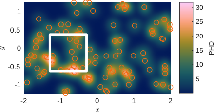
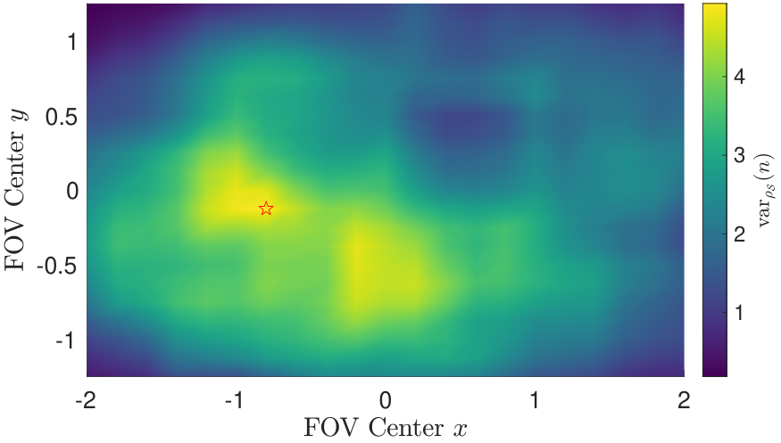
The objective of the sensor control problem is to place the fov, comprised of a square of dimensions, in the roi (Figure 9) such that the variance of object cardinality inside the fov is maximized. This objective can be interpreted as placing the fov in a region of the roi where the object cardinality is most uncertain. A related objective which minimizes the variance of the global cardinality using CB-MeMBer predictions was first proposed in [5]. For each candidate fov placement, the fov cardinality pmf is given by (90) and is efficiently computed using (92). The variance of the resulting pmf is shown as a function of the fov center location in Figure 10. The optimal fov center location is found to be .
A compelling result is that, by virtue of the bounded fov geometry, spatial information is encoded in the fov cardinality pmf. It can be seen that the optimal fov (Fig. 9) has boundary segments (lower half of left boundary and right half of lower boundary) that bisect clusters of mb components. These boundary segments divide the components’ single-object densities such that significant mass appears inside and outside the fov, increasing the overall fov cardinality variance.
VIII Conclusions
This paper presents an approach for incorporating bounded fov (fov) geometry into state density updates and object cardinality predictions via finite set statistics. Inclusion/exclusion evidence such as negative information and soft evidence is processed in state density updates via a novel Gaussian splitting algorithm that recursively refines a gm approximation near the boundaries of the discrete fov geometry. Using fisst, cardinality probability mass functions that describe the probability that a given number of objects exist inside the fov are derived. The approach is presented for representative labeled and unlabeled random finite set distributions and, thus, is applicable to a wide range of tracking, perception, and sensor planning problems.
References
- [1] R. P. Mahler, Statistical Multisource-Multitarget Information Fusion. Artech House Boston, 2007.
- [2] B.-N. Vo, B.-T. Vo, and D. Phung, “Labeled random finite sets and the Bayes multi-target tracking filter,” IEEE Transactions on Signal Processing, vol. 62, no. 24, pp. 6554–6567, 2014.
- [3] S. Reuter, B.-T. Vo, B.-N. Vo, and K. Dietmayer, “The labeled multi-Bernoulli filter,” IEEE Transactions on Signal Processing, vol. 62, no. 12, pp. 3246–3260, 2014.
- [4] Á. F. García-Fernández, Y. Xia, K. Granström, L. Svensson, and J. L. Williams, “Gaussian implementation of the multi-Bernoulli mixture filter,” in 2019 22nd International Conference on Information Fusion (FUSION), 2019.
- [5] H. G. Hoang and B.-T. Vo, “Sensor management for multi-target tracking via multi-Bernoulli filtering,” Automatica, vol. 50, no. 4, pp. 1135–1142, 2014. [Online]. Available: http://dx.doi.org/10.1016/j.automatica.2014.02.007
- [6] M. Beard, B.-T. Vo, B.-N. Vo, and S. Arulampalam, “Void probabilities and Cauchy-Schwarz divergence for generalized labeled multi-Bernoulli models,” IEEE Transactions on Signal Processing, vol. 65, no. 19, pp. 5047–5061, 2017.
- [7] X. Wang, R. Hoseinnezhad, A. K. Gostar, T. Rathnayake, B. Xu, and A. Bab-Hadiashar, “Multi-sensor control for multi-object Bayes filters,” Signal Processing, vol. 142, pp. 260–270, 2018. [Online]. Available: http://dx.doi.org/10.1016/j.sigpro.2017.07.031
- [8] S. Ferrari, R. Fierro, B. Perteet, C. Cai, and K. Baumgartner, “A geometric optimization approach to detecting and intercepting dynamic targets using a mobile sensor network,” SIAM Journal on Control and Optimization, vol. 48, no. 1, pp. 292–320, January 2009. [Online]. Available: https://doi.org/10.1137/07067934X
- [9] H. Wei and S. Ferrari, “A geometric transversals approach to sensor motion planning for tracking maneuvering targets,” IEEE Transactions on Automatic Control, vol. 60, no. 10, pp. 2773–2778, 2015.
- [10] S. Gehly, B. A. Jones, and P. Axelrad, “Search-detect-track sensor allocation for geosynchronous space objects,” IEEE Transactions on Aerospace and Electronic Systems, vol. 54, no. 6, pp. 2788–2808, 2018.
- [11] A. Buonviri, M. York, K. A. LeGrand, and J. Meub, “Survey of challenges in labeled random finite set based distributed multi-sensor multi-object tracking,” in 2019 IEEE Aerospace Conference, 2019.
- [12] K. A. LeGrand, P. Zhu, and S. Ferrari, “Cell Multi-Bernoulli (Cell-MB) Sensor Control for Multi-Object Search-While-Tracking (SWT),” IEEE Transactions on Pattern Analysis and Machine Intelligence, pp. 1–14, 2022.
- [13] ——, “A random finite set sensor control approach for vision-based multi-object search-while-tracking,” in 2021 24th International Conference on Information Fusion (FUSION), 2021.
- [14] T. Li, V. Elvira, H. Fan, and J. M. Corchado, “Local-Diffusion-Based Distributed SMC-PHD Filtering Using Sensors With Limited Sensing Range,” IEEE Sensors Journal, vol. 19, no. 4, pp. 1580–1589, 15 Feb.15, 2019.
- [15] K. Da, T. Li, Y. Zhu, and Q. Fu, “Gaussian Mixture Particle Jump-Markov-CPHD Fusion for Multitarget Tracking Using Sensors With Limited Views,” IEEE Transactions on Signal and Information Processing over Networks, vol. 6, pp. 605–616, 2020.
- [16] L. Gao, G. Battistelli, and L. Chisci, “Fusion of Labeled RFS Densities With Different Fields of View,” IEEE Transactions on Aerospace and Electronic Systems, pp. 1–16, 2022.
- [17] B. Wang, S. Li, G. Battistelli, L. Chisci, and W. Yi, “Multi-Agent Fusion With Different Limited Fields-of-View,” IEEE Transactions on Signal Processing, vol. 70, pp. 1560–1575, 2022.
- [18] W. Koch, “On exploiting ‘negative’ sensor evidence for target tracking and sensor data fusion,” Information Fusion, 2007.
- [19] I. R. Goodman, R. P. Mahler, and H. T. Nguyen, Mathematics of Data Fusion. Kluwer Academic Publishers, 1997.
- [20] A. Gning, B. Ristic, and L. Mihaylova, “Bernoulli particle/box-particle filters for detection and tracking in the presence of triple measurement uncertainty,” IEEE Transactions on Signal Processing, vol. 60, no. 5, pp. 2138–2151, 2012.
- [21] B. Ristic, Particle Filters for Random Set Models. Springer, New York, NY, 2013.
- [22] A. N. Bishop and B. Ristic, “Fusion of spatially referring natural language statements with random set theoretic likelihoods,” IEEE Transactions on Aerospace and Electronic Systems, vol. 49, no. 2, pp. 932–944, 2013.
- [23] B. Ristic, B.-T. Vo, B.-N. Vo, and A. Farina, “A tutorial on Bernoulli filters: Theory, implementation and applications,” IEEE Transactions on Signal Processing, vol. 61, no. 13, pp. 3406–3430, 2013.
- [24] M. S. Arulampalam, S. Maskell, N. Gordon, and T. Clapp, “A tutorial on particle filters for online nonlinear/non-Gaussian Bayesian tracking,” IEEE Transactions on Signal Processing, vol. 50, no. 2, pp. 174–188, 2002.
- [25] B.-N. Vo, S. Singh, and A. Doucet, “Sequential Monte Carlo methods for multitarget filtering with random finite sets,” IEEE Transactions on Aerospace and Electronic Systems, vol. 41, no. 4, pp. 1224–1245, 2005.
- [26] T. L. Song, D. Musicki, and K. D. Sol, “Target tracking with target state dependent detection,” IEEE Transactions on Signal Processing, vol. 59, no. 3, pp. 1063–1074, 2011.
- [27] N. R. Ahmed, E. M. Sample, and M. Campbell, “Bayesian multicategorical soft data fusion for human-robot collaboration,” IEEE Transactions on Robotics, vol. 29, no. 1, pp. 189–206, 2013.
- [28] B. Wei and B. Nener, “Distributed space debris tracking with consensus labeled random finite set filtering,” Sensors, vol. 18, pp. 1–26, 2018.
- [29] K. A. LeGrand and S. Ferrari, “The role of bounded fields-of-view and negative information in finite set statistics (FISST),” in Proceedings of the 2020 23rd International Conference on Information Fusion (FUSION), July 2020, pp. 1–9.
- [30] K. A. Baumgartner, S. Ferrari, and A. V. Rao, “Optimal control of an underwater sensor network for cooperative target tracking,” IEEE Journal of Oceanic Engineering, vol. 34, no. 4, pp. 678–697, 2009.
- [31] B.-N. Vo and W.-K. Ma, “The Gaussian mixture probability hypothesis density filter,” IEEE Transactions on Signal Processing, vol. 54, no. 11, pp. 4091–4104, Nov 2006.
- [32] K. A. LeGrand and K. J. DeMars, “Relative multiple space object tracking using intensity filters,” in Proceedings of the 2015 18th International Conference on Information Fusion (FUSION), 2015, pp. 1253–1261.
- [33] M. F. Huber, T. Bailey, H. Durrant-Whyte, and U. D. Hanebeck, “On entropy approximation for Gaussian mixture random vectors,” IEEE International Conference on Multisensor Fusion and Integration for Intelligent Systems, pp. 181–188, 2008.
- [34] K. J. DeMars, R. H. Bishop, and M. K. Jah, “Entropy-based approach for uncertainty propagation of nonlinear dynamical systems,” Journal of Guidance, Control, and Dynamics, vol. 36, no. 4, pp. 1047–1057, 2013. [Online]. Available: http://arc.aiaa.org/doi/10.2514/1.58987
- [35] M. F. Huber, “Adaptive Gaussian mixture filter based on statistical linearization,” in 14th International Conference on Information Fusion, 2011, pp. 1–8.
- [36] K. Tuggle and R. Zanetti, “Automated Splitting Gaussian Mixture Nonlinear Measurement Update,” Journal of Guidance, Control, and Dynamics, vol. 41, no. 3, pp. 1–10, 2018.
- [37] R. P. Mahler, Advances in Statistical Multisource-Multitarget Information Fusion. Artech House, 2014.
- [38] N. Patwari, J. N. Ash, S. Kyperountas, A. O. Hero, R. L. Moses, and N. S. Correal, “Locating the nodes: cooperative localization in wireless sensor networks,” IEEE Signal Processing Magazine, vol. 22, no. 4, pp. 54–69, 2005.
- [39] R. Tse and M. Campbell, “Human–Robot Communications of Probabilistic Beliefs via a Dirichlet Process Mixture of Statements,” IEEE Transactions on Robotics, vol. 34, no. 5, pp. 1280–1298, 2018.
- [40] D. L. Alspach and H. W. Sorenson, “Nonlinear bayesian estimation using Gaussian sum approximations,” IEEE Transactions on Automatic Control, vol. 17, no. 4, pp. 439–448, 1972.
- [41] M. West, “Approximating posterior distributions by mixtures,” Journal of the Royal Statistical Society: Series B (Methodological), vol. 55, no. 2, pp. 409–422, jan 1993.
- [42] A. R. Runnalls, “Kullback-Leibler approach to Gaussian mixture reduction,” IEEE Transactions on Aerospace and Electronic Systems, vol. 43, no. 3, pp. 989–999, 2007.
- [43] D. J. Salmond, “Mixture reduction algorithms for point and extended object tracking in clutter,” IEEE Transactions on Aerospace and Electronic Systems, vol. 45, no. 2, pp. 667–686, 2009.
- [44] D. F. Crouse, P. Willett, K. R. Pattipati, and L. Svensson, “A look at Gaussian mixture reduction algorithms,” in Proceedings of the 2011 14th International Conference on Information Fusion, 2011, pp. 1–8.
- [45] E. Delande, M. Üney, J. Houssineau, and D. E. Clark, “Regional variance for multi-object filtering,” IEEE Transactions on Signal Processing, vol. 62, no. 13, pp. 3415–3428, 2014.
- [46] E. Delande, J. Houssineau, and D. Clark, “Regional variance in target number: Analysis and application for multi-Bernoulli point processes,” in IET Conference on Data Fusion & Target Tracking 2014: Algorithms and Applications. Institution of Engineering and Technology, 2014, pp. 4.2–4.2.
- [47] K. F. Riley, M. P. Hobson, and S. J. Bence, Mathematical Methods for Physics and Engineering: A Comprehensive Guide. Cambridge University Press, 2006.
- [48] J. L. Williams, “Marginal multi-Bernoulli filters: RFS derivation of MHT, JIPDA, and association-based MeMBer,” IEEE Transactions on Aerospace and Electronic Systems, vol. 51, no. 3, pp. 1664–1687, 2015.
- [49] M. Fernandez and S. Williams, “Closed-form expression for the Poisson-Binomial probability density function,” IEEE Transactions on Aerospace and Electronic Systems, vol. 46, no. 2, pp. 803–817, 2010.
- [50] R. P. Mahler, “PHD filters of higher order in target number,” IEEE Transactions on Aerospace and Electronic Systems, vol. 43, no. 4, pp. 1523–1543, October 2007.
- [51] B.-T. Vo and B.-N. Vo, “Labeled random finite sets and multi-object conjugate priors,” IEEE Transactions on Signal Processing, vol. 61, no. 13, pp. 3460–3475, 2013.
Appendix A Inclusion Consistency Example
Consider a plane of constant –that is, and . As pictured in Fig. 11, the index denotes the ninth grid plane from the bottom. To evaluate inclusion/exclusion consistency in this plane, an arbitrary reference point is selected as (where the corresponding indices are and ). Note that this reference index tuple belongs to (depicted by the set of orange dots) and lies in the plane of constant .
It is apparent from Fig. 11 that . Thus, the corresponding component inclusion variable (25) for the selected reference point is
| (102) |
In the following inclusion/exclusion consistency check, which follows from (27), the inclusion variables are computed for all remaining points in the plane and compared to :
| (103) |
where it is noted that ranges from two to fourteen in the considered plane (in which there are thirteen corresponding orange dots). Thus, signifies that the plane is indeed consistently inside or consistently outside the fov, the latter of which is easily verified by inspecting Fig. 11.
Appendix B Taylor Series Expansion About Means
Equation (55) can be written compactly as
| (104) | ||||
| (105) |
where
| (106) |
and where the functional dependence of on the fov and measurement is omitted for brevity. The function can be approximated locally by a Taylor series expansion about a given component mean as
| (107) |
To zeroth order, , such that
| (108) |
Appendix C Proof of Proposition 3
Let . Then, (89) can be rewritten as
| (109) |
where denotes the (unordered) set and denotes the (ordered) sequence , where the -tuple index set and is a permutation of .
| (110) |
The last sum can be written in terms of label index sets as
| (111) | ||||
where the innermost sum is taken over all mutually disjoint subsets , such that . Distributing terms from the second summation,
| (112) | ||||
Because , then and the integral on becomes a product of integrals on , such that
| (113) | ||||
Now note that the result of the innermost sum does not depend the permutation order of . Thus the property [51, Lemma 12], which states that for an arbitrary symmetric function ,
| (114) |
is applied, yielding
| (115) | ||||
The term is non-zero only when the combined cardinality of and is equal to —the index of the outermost sum. Thus, the outermost sum is absorbed by the second sum to give (90).