A Supervised Tensor Dimension Reduction-Based Prognostic Model for Applications with Incomplete Imaging Data
Abstract
Imaging data-based prognostic models focus on using an asset’s degradation images to predict its time-to-failure (TTF). Most image-based prognostic models have two common limitations. First, they require degradation images to be complete (i.e., images are observed continuously and regularly over time). Second, they usually employ an unsupervised dimension reduction method to extract low-dimensional features, and then use the features for TTF prediction. Since unsupervised dimension reduction is conducted on the degradation images without the involvement of TTFs, there is no guarantee that the extracted features are effective for failure time prediction. To address these challenges, this article develops a supervised tensor dimension reduction-based prognostic model. The model first proposes a supervised dimension reduction method for tensor data. It uses historical TTFs to guide the detection of a tensor subspace to extract low-dimensional features from high-dimensional incomplete degradation imaging data. Next, the extracted features are used to construct a prognostic model based on (log)-location-scale regression. An optimization algorithm for parameter estimation is proposed and analytical solutions are discussed. Simulated data and a real-world data set are used to validate the performance of the proposed model.
Keywords: Supervised dimension reduction, missing data, tensor, failure time prediction
1 Introduction
Degradation is an irreversible process of damage accumulation that results in the failure of engineering systems/assets/components (Bogdanoff and Kozin 1985). Although it is usually challenging to observe a physical degradation process, there often are some manifestations associated with degradation processes that can be monitored by sensing technology, which yields data known as degradation data/signals. Degradation data contains the health condition of engineering assets; thus, if modeled properly, they can be used to predict the assets’ time-to-failure (TTF) via a process known as prognostic. Many prognostic models have been developed in the literature, most of which focus on using time series-based degradation data (Ye et al. 2014; Ye and Chen 2014; Hong and Meeker 2010; Hong and Meeker 2013; Shu et al. 2015; Liu et al. 2013; Gebraeel et al. 2005; Wang et al. 2022). Recently, prognostic models with imaging-based degradation data have been investigated and attracted more and more attention. This is because comparing with time-series data, imaging data usually contains much richer information of the object being monitored, and imaging sensing technologies are noncontact and thus they can usually be easily deployed. One example of imaging-based degradation data is the infrared image stream that measures the change of temperature distribution of a thrust bearing during its degradation process over time (Fang et al. 2019; Aydemir and Paynabar 2019; Dong et al. 2021; Jiang et al. 2022a; Wang et al. 2021). Another example is the images used to measure the performance degradation of infrared systems such as rotary-wing drones (Dong et al. 2021).
The existing imaging-based prognostic methods include deep learning-based models and statistical learning methods. Examples of the deep learning-based models designed for TTF prediction using imaging data include the ones developed by Aydemir and Paynabar 2019; Yang et al. 2021; Dong et al. 2021, Jiang et al. 2022a, Jiang et al. 2022b, and Jiang et al. 2023. Although these models have worked relatively well, they usually provide point estimations of failure times, and it is challenging for them to quantify the uncertainty of predicted TTFs (e.g., providing a failure time distribution). This limits their applicability since the subsequent decision-making analysis such as maintenance/inventory/logistic optimization requires prognostic models to provide a distribution of the predicted TTF. Also, deep learning-based prognostic models often require a relatively large number of historical samples for model training, which cannot be satisfied by many real-world applications with limited historical data. One example of statistical learning methods for image-based prognostic is the penalized (log)-location-scale (LLS) tensor regression proposed by Fang et al. 2019. The model first employs multilinear principal component analysis (MPCA) (Lu et al. 2008) to reduce the dimension of high-dimensional imaging-based degradation data, which yields a low-dimensional feature tensor for each asset. Next, it constructs a prognostic model by regressing an asset’s TTF against its low-dimensional feature tensor using LLS regression. In the same article, Fang et al. 2019 have also proposed several benchmarking prognostic models that use imaging-based degradation data for TTF prediction. These models also first employ a dimension reduction method such as functional principal component analysis (FPCA) (Ramsay and Silverman 2005), principal component analysis (PCA) (Abdi and Williams 2010), or B-Spline (Prautzsch et al. 2002), to reduce the dimension of degradation data and then use low-dimensional features to build an LLS regression model for prognostic. Although the aforementioned statistical learning-based prognostic models can provide a distribution for the predicted TTF, and their effectiveness have been well investigated, they share two common limitations.
The first limitation is that they assume imaging-based degradation data (including historical data for model training and real-time data for model test) are complete, which means images from all the assets should be collected continuously and regularly with the same sampling time interval (see Figure 1 (a) for an example). In reality, however, engineering assets often operate in harsh environments that significantly impact the quality of collected data due to errors in data acquisition, communication, read/write operations, etc. As a result, degradation images often contain significant levels of missing observations, which is known as incomplete/missing imaging data (see Figure 1 (b) for an example). Such data incompleteness poses a significant challenge for the parameter estimation of existing statistical learning-based prognostic models.
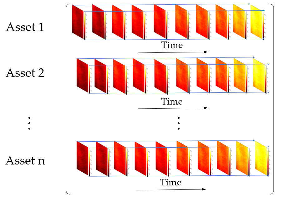
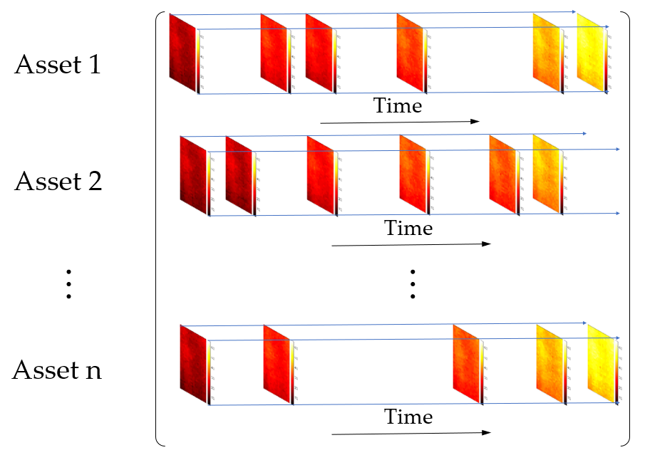
The second common limitation for the existing statistical learning-based prognostic models for applications with imaging data is that they employ unsupervised dimension reduction methods for feature extraction, so there is no guarantee that the extracted features are effective for the subsequent TTF prediction. Specifically, they first use unsupervised dimension reduction methods such as FPCA, PCA, and B Spline to extract features, which are then used to construct prognostic models. Since feature extraction and prognostic model construction are two sequential steps, and no TTF information gets involved in the feature extraction process, it is possible that the extracted features may not be most suitable for predicting TTFs.
To address the aforementioned challenges, this article proposes a supervised dimension reduction-based prognostic model that uses an asset’s incomplete degradation images to predict its TTF. Similar to the existing statistical learning-based prognostic models, the proposed model also consists of two steps: feature extraction and prognostic model construction. However, unlike the existing models, feature extraction in this article is achieved by developing a new supervised tensor dimension reduction method, which uses historical TTFs to supervise the feature extraction process such that the extracted features are more effective for the subsequent TTF prediction. In addition, unlike the existing unsupervised dimension reduction methods that only work for complete imaging data, the proposed supervised dimension reduction method works for both complete and incomplete degradation image streams.
The proposed supervised dimension reduction method works as follows: First, it detects a low-dimensional tensor subspace in which the high-dimensional degradation image streams are embedded. This is achieved by constructing an optimization criterion that comprises a feature extraction term and a regression term. The first term extracts low-dimensional features from complete/incomplete degradation image streams of training assets, and the second term builds the connection between these assets’ TTFs and the extracted features using LLS regression. LLS regression has been widely used in reliability engineering and survival analysis. It includes a variety of TTF distributions, such as (log)normal, (log)logistic, smallest extreme value, and Weibull, etc., which cover most of the TTF distributions in reality (Doray 1994). Since historical TTFs are used to supervise the feature extraction process, it is expected that the extracted features are more effective for the subsequent prognostic. Solving the optimization criterion of the proposed supervised tensor dimension reduction method yields a set of tensor basis matrices that span the low-dimensional tensor subspace for dimension reduction. We then expand both the historical degradation images in the training data set and real-time degradation images from an asset operating in the field (i.e., test data) using the set of tensor basis matrices to extract the low-dimensional tensor features of the training assets and the test asset. The TTFs of the training assets are then regressed against their tensor features using LLS regression, and the parameters are estimated using maximum likelihood estimation. After that, the tensor features of the test asset are fed into the LLS regression model, and its TTF distribution is predicted.
To solve the optimization criterion of the proposed supervised dimension reduction method, we will first transfer the criterion into a block multiconvex problem. Next, we will propose a block updating algorithm, which cyclically optimizes one block parameters while keeping other blocks fixed until convergence. In addition, we will demonstrate that when TTFs follow normal or lognormal distributions, each sub problem of the block updating algorithm has a closed-form solution, no matter the degradation image streams are complete or incomplete.
The rest of this paper is orginized as follows. Section 2 presents the supervised tensor dimension reduction-based prognostic method. Section 3 introduces the block updating algorithm and closed-form solutions when TTFs follow normal/lognormal distributions. Sections 5 and 6 validate the effectiveness of the proposed prognostic model using a simulated dataset and data from a rotating machinery, respectively. Section 7 concludes.
2 The Methodology
In this section, we will introduce the proposed supervised tensor dimension reduction-based prognostic model for applications with incomplete imaging data. In subsection 2.1, we will present some basic tensor notations and definitions. subsection 2.2 introduces the supervised tensor dimension reduction method. In subsection 2.3, we will discuss the construction of prognostic model and how to predict the TTF of an asset operating in the field using its real-time degradation imaging data.
2.1 Preliminaries
In this section, we introduce some basic notations and definitions of tensor operations that are used throughout the article. The order of a tensor is the number of dimensions, also known as ways or modes. Vectors (1 order tensors) are denoted by lowercase boldface letters, e.g., . Matrices (2 order tensors) are denoted by boldface uppercase letters, e.g., . Higher-order tensors (order is 3 or larger) are denoted by calligraphic letters, e.g., . Indices are denoted by lowercase letters whose range is from 1 to the uppercase letter of the index, e.g., . An th-order tensor is denoted as , where represents the th mode of . The th entry of is denoted by . A fiber of is a vector defined by fixing every index but one. A matrix column is a mode-1 fiber and a matrix row is a mode-2 fiber. The vectorization of , denoted by vec(), stacks all the entries of into a column vector. The mode- matricization of a tensor is denoted by , which arranges the mode- fibers to be the columns of the resulting matrix. The th mode product of a tensor and a matrix , denoted by , is a tensor whose entry is . The Kronecker product of two matrices and is an block matrix:
If and have the same number of columns , then the Khatri-Rao product is defined as the column-wise Kronecker product: . If and are vectors, then . More details about tensor notations and operators can be found in Kolda and Bader 2009.
2.2 The Supervised Tensor Dimension Reduction Method
We assume that there exists a historical data set for model training. The data set consists of the degradation image streams of failed assets along with their TTFs, which are denoted as and , respectively, where . For the convenience of introducing the dimension reduction method, we convert the 3D degradation image streams from all the assets to a 4D tensor , where the sample size is the 4th mode. Similarly, we let be the vector containing all the TTFs of the assets.
Out of the entries of , we use a subset to denote the indices of the missing ones. To model the missing data, we define a projection operator as follows:
| (1) |
where is the -th entry of the 4D tensor . To recover the missing entries in tensor , we may employ the following Tucker decomposition-based tensor completion method (Filipović and Jukić 2015; Liu et al. 2012; Xu et al. 2013):
| (2) |
where is the Frobenius norm, , , are three factor matrices, is the low-dimensional core tensor, and is the n-mode product of a tensor with a matrix. The tensor completion criterion (2) can be seen as an unsupervised dimension reduction method for tensor data with missing entries. This is because the degradation image tensor is a 4-order tensor, which resides in the tensor (multilinear) space , where are the 4 vector (linear) spaces; can be seen as a feature tensor that resides in the tensor space . Usually, we have , , and for degradation imaging data due to the high spatio-temporal correlation among pixels. This implies that the dimension of the image stream from the th asset is reduced from to , where .
Although criterion (2) can be seen as a dimension reduction method, there is no guarantee that the extracted low-dimensional feature tensor is effective for the subsequent TTF prediction. To address this challenge, we propose the following supervised dimension reduction method by combining a tensor completion term and an LLS regression term:
| (3) |
where is the vector containing all the TTFs of the assets in the training data set. The matrix is the mode-4 matricization of the low-dimensional feature tensor , the th row of which represents the vectorization of the th asset’s feature tensor, . is the intercept, and is the regression coefficient vector. is an vector whose entries are all ones. is the negative log-likelihood function of a location-scale distribution. For example, if TTFs follow normal distributions, then , where , where is the th row of , and is the TTF of asset ; if TTFs follow logistic distributions, then ; if TTFs follow small extreme value (SEV) distributions, then . For assets whose TTFs follow log-location-scale distributions, we may transfer them to the corresponding location-scale distributions by taking their logarithm such that criterion (3) can still be used. For example, log-normal, log-logistics, and Weibull distributions can be transferred to normal, logistics, and SEV distributions, respectively. is a weight and is the Frobenius norm.
In criterion (3), the first term is tensor completion from (2), which reduces the dimension of high-dimensional incomplete degradation image streams and extracts low-dimensional tensor features. The second term is LLS regression, which regresses each asset’s TTF against its tensor features extracted by the first term. By jointly optimizing the two terms, it is expected that the extracted features are effective for TTF prediction. However, it is challenging to solve criterion (3) since it is neither convex nor block multi-convex. An optimization problem is block multi-convex when its feasible set and objective function are generally non-convex but convex in each block of variables (Xu and Yin 2013). Thus, to simplify the development of optimization algorithms for model parameter estimation, we first transform criterion (3) to a block multi-convex one. Specifically, we apply the following re-parameterization: . As a result, criterion (3) can be re-expressed as follows:
| (4) |
where, for TTFs following normal distributions, and , where is the th row of and is the TTF of asset ; for TTFs following logistics distributions, and for TTFs following SEV distributions.
The optimization algorithm to solve criterion (4), the value of the weight , and the dimension of the low-dimensional tensor subspace will be discussed in Sections 3 and 4. Solving the optimization criterion (4) using historical training data yields a set of basis matrices , which contains basis vectors of the -mode linear space , basis vectors of the -mode linear space , and basis vectors of the -mode linear space , respectively. The three linear subspaces form the low-dimensional tensor subspace detected by the proposed supervised dimension reduction method.
One of the assumptions of the proposed supervised tensor dimension reduction method in criterion (4) is that the TTF of the asset follows a distribution from the LLS family. This is reasonable since the LLS family includes a variety of TTF distributions, such as (log)normal, (log)logistic, smallest extreme value, and Weibull, etc., which cover most of the TTF distributions in engineering applications (Doray 1994). Another assumption is that there is a linear relationship between the location parameter and predictors (i.e., degradation signals or their features in this article). Specifically, the location parameters in criterion (3) are expressed as , which are linear weighted combinations of the rows of ). This assumption is widely used in LLS regression (Doray 1994; Fang et al. 2019). However, if a simple linear weighted combination is not adequate to characterize the association between the location parameter and degradation signal features, a high-order polynomial relationship can be constructed (Hastie et al. 2009). By doing so, we can model a more complex association between the location parameter and features. More importantly, the incorporation of high-order polynomial terms into the proposed supervised tensor dimension reduction method does not affect the effectiveness of the optimization algorithms for parameter estimation to be discussed in Sections 3 and 4.
2.3 Prognostic Model Construction and Real-Time TTF Prediction
In this subsection, we discuss how to build a prognostic model based on the supervised dimension reduction method proposed in Section 2.2, and how to predict the TTF distribution of an asset operating in the field using its real-time degradation image data.
Similar to Section 2.2, we denote the training data set as , where is the number of failed assets in the training data set. Notice that might not be the same as for two assets and , . This is because different asset’s failure times (i.e., TTFs) are different, and usually no image data can be collected beyond an asset’s failure time since the asset is stopped for maintenance or replace once it is failed. In addition to the training data, we denote the degradation image stream of a test asset by time as . The objectives of this subsection include 1) constructing a prognostic model and estimating its parameters using in the training data set, and 2) using the estimated prognostic model to predict the TTF (denoted as ) of the test asset based on its degradation image stream .
We first use the proposed supervised dimension reduction method to extract low-dimensional features of both the training and test assets. Specifically, as discussed in Section 2.2, we first construct a 4D tensor using the degradation image streams of the training assets, where . Note that is an incomplete tensor no matter the image streams from the training assets are complete or incomplete. This is because the TTFs of training assets are different, and thus not all the training assets have images. To detect the low-dimensional tensor subspace in which the high-dimensional degradation images are embedded, we solve optimization criterion (4) by using training data , where . This yields basis matrices , which form the low-dimensional tensor subspace . To extract the low-dimensional features of the training and test assets, we expand the image streams in the low-dimensional tensor subspace using the basis matrices . This is achieved by solving the following optimization criteria:
| (5) |
| (6) |
where are the low-dimensional feature tensors of the assets in the training data set, and is the low-dimensional feature tensor of the test asset.
Next, we construct a prognostic model using the low-dimensional feature tensors of the assets in the training data set (i.e., ) along with their TTFs . Specifically, we build the following LLS regression model:
| (7) |
where is the vectorization of . and are the regression coefficients, is the scale parameter, and is the random noise term with a standard location-scale probability density function . For example, for a normal distribution and for an SEV distribution. The parameters in criterion (7) can be estimated by solving the following optimization problem:
| (8) |
where is the negative log-likelihood function of a location-scale distribution, and , and is the negative log-likelihood function. We conduct the following reparameterization to transform the optimization to be a convex one: :
| (9) |
Solving (9) provides the estimated parameters , which can be transformed back to the estimation of the parameters in the LLS regression model: , and . As a result, the fitted LLS regression model is , where and are respectively the estimated location and scale parameters.
Finally, we feed the extracted low-dimensional feature tensor of the test asset into the estimated LLS regression model to predict the asset’s TTF distribution: .
3 The Optimization Algorithm
In this section, we discuss how to solve the supervised tensor dimension reduction method proposed in section 2.2. In subsection 3.1, we develop a Block Updating Algorithm to solve criterion (4). The algorithm splits the unknown parameters in criterion (4) into several blocks, and it cyclically optimizes one block parameter while keeping other blocks fixed until convergence. The sub-optimization problem for each block is convex, so the convergence of the block updating algorithm is guaranteed. In subsection 3.2, we discuss the initialization of the proposed algorithm and hyperparameter tuning.
3.1 The Block Updating Algorithm
The Block Updating Algorithm first splits the unknown parameters in criterion (4) into 5 blocks, i.e., and . It then cyclically optimizes one block of parameters each time while keeping other blocks fixed.
Specifically, at the th iteration, is updated by solving the following optimization problem while keeping other blocks (i.e., ) fixed:
| (10) |
Similarly, the remaining blocks are updated as follows:
| (11) |
| (12) |
| (13) |
| (14) |
We summarize the Block Updating Algorithm in Algorithm 1 below. The convergence criterion can be set as , where is the value of the objective function in criterion (4), and is a small number. It is easy to show that sub problems (10), (11), and (12) are convex. For normal, logistic, and SEV distributions, their negative log-likelihood functions are also convex, so objective functions (13) and (14) are convex as well. As a result, the Block Updating Algorithm converges to a stationary point of criterion (4).
3.2 Initialization and Hyperparameter Tuning
To run Algorithm 1, we need to initialize the parameters . The initialization can be accomplished randomly or heuristically. In this article, we propose a heuristic initialization method. Specifically, if tensor has no missing entries, MPCA (Lu et al. 2008) is applied to tensor , which yields . Next, we compute by solving . Finally, are computed by solving , where is the mode-4 matricization of . If tensor has missing values, a tensor completion method (Filipović and Jukić 2015; Liu et al. 2012; Xu et al. 2013) can be conducted before applying MPCA.
In addition to the initialization, the hyperparameter parameters including the weight and the dimension of tensor subspace also need to be pre-determined. It is known that controls the weights of the feature extraction term and the regression term, and . To select an appropriate weight parameter, we will first split the range into intervals equally, which yields . Next, we employ cross-validation to select the weight that achieves the highest prediction accuracy. If the weight at the boundary is selected (i.e., or ), we further split the interval closest to the boundary and conduct cross-validation again. For example, if is chosen as the best weight, we will split into intervals equally and re-conduct the cross-validation. This process is repeated until a non-boundary weight is selected. Of course, a maximum number of repetitions needs to be set to control the computational time.
The values of can be determined using cross-validation as well. To be specific, we may try a certain number of candidate values for and run Algorithm 1 to extract low-dimensional features, which are then used to build the prognostic model discussed in Section 2.3 for TTF prediction. The values which achieve the smallest prediction error will be chosen. It is known that there usually exists high spatio-temporal correlations among degradation image streams (Fang et al. 2019), so the dimension of the tensor subspace is usually low, which helps reduce the computation intensity of model selection. The values of can also be determined heuristically. For example, if MPCA is employed for parameter initialization, then the fraction-of-variance-explained (Lu et al. 2008) can be used to determine the dimension of tensor subspace.
4 Analytical Solutions
In this section, we discuss the closed-form solutions of optimization problems (10), (11), (12), (13), and (14) in Algorithm 1. Specifically, we will discuss the solutions when degradation image streams are complete and incomplete in Sections 4.1 and 4.2, respectively. For simplicity, we will remove the superscripts and .
4.1 Analytical Solutions for Complete Data
4.1.1 Solution procedure for
When degradation image streams are complete (i.e., the 4D image tensor in criterion (4) has no missing entries), we have the following proposition, which provides the analytical solution to problem (10).
Proposition 1
If the 4D tensor has no missing values, optimization problem (10) has the following analytical solution
where is the mode-1 matricization of , , is the mode-1 matricization of , and the operator “” represents multiplication.
4.1.2 Solution procedure for
When degradation image streams are complete, the proposition below gives the analytical solution to problem (11).
Proposition 2
If the 4D tensor has no missing values, optimization problem (11) has the following analytical solution
where is the mode-2 matricization of , , and is the mode-2 matricization of .
4.1.3 Solution procedure for
When degradation image streams are complete, the proposition below provides the analytical solution to problem (12).
Proposition 3
If the 4D tensor has no missing values, optimization problem (12) has the following analytical solution
where is the mode-3 matricization of , , and is the mode-3 matricization of .
4.1.4 Solution procedure for
For general LLS distributions, there is no closed-form solution for . As a result, we may use existing algorithms (Doray 1994) or convex optimization packages to solve problem (13). However, if the TTF follows a Normal (or lognormal) distribution, we may replace the negative log-likelihood term in criterion (3) with a mean squared error-based loss function, which results in the following optimization criterion:
| (15) |
4.1.5 Solution procedure for
For general LLS distributions, there is no closed-form solution for either. Therefore, we may use existing convex optimization packages to solve problem (14). However, if the TTF follows a Normal (or lognormal) distribution, according to criterion (15), problem (14) is equivalent to
| (16) |
which has an analytical solution as suggested by Proposition 4.
Proposition 4
If the 4D tensor has no missing values, optimization problem (16) has the following analytical solution
where is the mode-4 matricization of , is the mode-4 matricization of .
The proof of Propositions 1, 2, 3, and 4 can be found in the Appendix
4.2 Analytical Solutions for Incomplete Data
In this subsection, we discuss the closed-form solutions for optimization problems (10), (11), (12), (13), and (14) when the degradation tensor in criterion (4) is incomplete. We consider the most general missing pattern, entry-wise missing, which means that any entry of can be missing. Thus, the indices of missing entries can be denoted as a subset .
4.2.1 Solution procedure for
When tensor has a general entry-wise missing structure, there is no closed-form solution for in optimization criterion (10). However, we may decompose criterion (10) into multiple sub-optimization problems, each of which has an analytical solution. To be specific, we first give the following lemma.
Lemma 1
Let , , and , the solution to criterion can be found by solving each row of separately–that is–solving as follows:
where is the th row of , is the th row of .
The proof of Lemma 1 can be found in the Appendix. Lemma 1 enables us to solve each column of matrices separately. Denote the th column of matrix as , we replace optimization problem (10) with sub problems by separately optimizing . Proposition 5 suggests that there is an analytical solution when optimizing .
Proposition 5
When optimizing the th column of in problem (10), we have the following analytical solution
where denotes the th row of , is a set consisting of the indices of available entries of , denotes a vector consisting of the available entries in the th row of , , is the mode-1 matricization of , and denotes a matrix comprises the columns of .
As mentioned earlier, when tensor has a general entry-wise missing structure, there is no closed-form solution for in optimization criterion (10). Therefore, we have to optimize each column of matrix separately using the analytical solution provided in Proposition 5. However, for image-based applications, the missing data in tensor are images but not entries, as illustrated in Figure 2(b). This yields an image-wise missing structure, which is a special case of the general entry-wise missing structure. For image streams with an image-wise missing structure, Proposition 6 suggests that in optimization criterion (10) can be estimated analytically as a whole, which means we do not have to optimize each of its columns separately.
Proposition 6
If the indices of tensor ’s missing entries can be denoted as , , where “” denotes all the indices in a dimension, then ’s mode-1 matricization has missing columns. Let be the set consisting of the indices of available columns in , then optimization problem (10) has the following analytical solution
where is a matrix consisting of the columns of , , is the mode-1 matricization of , and denotes a matrix constituting the columns of .
4.2.2 Solution procedure for
Similar to , there is no closed-form solution for in optimization criterion (11) when tensor has a general entry-wise missing structure. However, Lemma 1 implies that we may also decompose optimization problem (11) into multiple sub-criteria, each of which has a closed-form solution. Specifically, denote the th column of matrix as , we can replace optimization problem (11) with sub problems by separately optimizing . Proposition 7 shows that there is an analytical solution for .
Proposition 7
When optimizing the th column of in problem (11), we have the following analytical solution
where denotes the th row of , is a set consisting of the indices of available entries of , is a vector consisting of the available entries in the th column of , , is the mode-2 matricization of , and denotes a matrix comprises the columns of .
Similar to , when tensor has the image-wise missing structure, we do not have to optimize each of the columns of separately. Proposition 8 below gives an analytical solution to when tensor has missing images.
Proposition 8
If the indices of tensor ’s missing entries can be denoted as , , where “” denotes all the indices in a dimension, then ’s mode-2 matricization has missing columns. Let be the set consisting of the indices of available columns in , then optimization problem (11) has the following analytical solution
where is a matrix consisting of the columns of , is the mode-2 matricization of , and denotes a matrix constituting the columns of .
4.2.3 Solution procedure for
There is no closed-form solution for in optimization criterion (12) when tensor has missing entries. Based on Lemma 1, we decompose optimization problem (12) into multiple sub-criteria, each of which has a closed-form solution. Denote the th column of matrix as , we replace optimization problem (12) with sub problems by separately optimizing respectively. Proposition 9 suggests that there is an analytical solution when optimizing .
Proposition 9
When optimizing the th column of in problem (12), we have the following analytical solution
where denotes the th row of , is a set consisting of the indices of available entries of , is a vector consisting of the available entries in the th row of , , is the mode-3 matricization of , and denotes a matrix comprises the columns of .
4.2.4 Solution procedure for
Whether tensor contains missing entries does not affect the methods for , and estimation. Therefore, the estimation methods discussed in Section 4.1.4 can still be used.
4.2.5 Solution procedure for
For general LLS distributions, there is no closed-form solution for . Therefore, we may use existing convex optimization packages to solve problem (14). However, if the TTF follows a Normal (or lognormal) distribution, problem (14) is equivalent to (16) (see Section 4.1.5 for details). Based on Lemma 1, we may optimize each row of separately. We denote the th row of matrix as , , and replace optimization problem (16) with sub problems–that is–separately optimizing . Proposition 10 suggests that there is an analytical solution when optimizing .
Proposition 10
When optimizing the th row of matrix in problem (16), we have the following analytical solution
where represents the th row of , denotes the set consisting of the indices of available entries in , is a vector consisting of the available entries in the th row of , and denotes a matrix comprising the columns of matrix .
The proof of all Propositions 5, 6, 7, 8, 9, and 10 can be found in the Appendix.
5 Numerical Studies
In this section, we validate the effectiveness of our proposed supervised tensor dimension reduction-based prognostic model using simulated data.
5.1 Data Generation
We generate degradation image streams for assets. The image stream from asset , which is denoted by , is generated from the following heat transfer equation:
| (17) |
where , represents the location of each image pixel. is the thermal diffusivity coefficient, which is randomly generated from a uniform distribution . is the time index. The initial and boundary conditions are set such that and . At each time , the image is recorded at locations , resulting in an matrix. Here, we set and , which yields 150 images of size 21 21 for each asset. This implies that the degradation image stream of each asset can be represented by a 21 21 150 tensor. In addition, an independent and identically distributed random noise is added to each pixel. Figure 2 demonstrates an example of some images with and without noise from one of the assets simulated in this study.
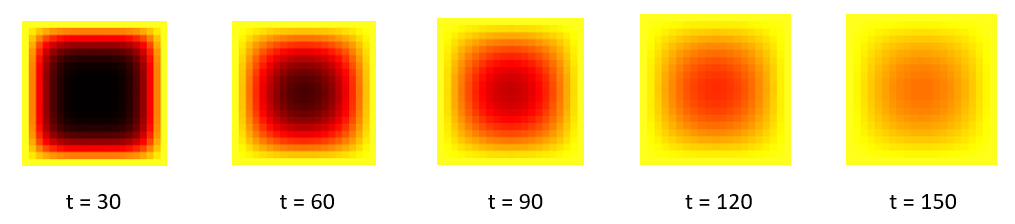
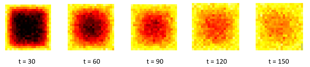
To determine the TTF of an asset, we first transform the asset’s tensor to a time series by taking the average pixel intensity of each image. The time series signal indicates how the average heat of the asset involves over time. Next, we let the TTF of the asset be the time point where the amplitude of the time series signal crosses a pre-defined soft failure threshold, which is set as in this study. Since the images of different assets are generated with different thermal diffusivity coefficients, the time points where their time series signals go beyond the threshold may be different. Thus, the TTF of different asset may also be different. To mimic reality, we truncate the image stream of each asset by keeping only the images observed before its TTF. In other words, any images observed after an asset’s TTF are removed from the image tensor of the asset. Such a truncation is normal in reality since an asset usually gets maintained or replaced once its degradation signal crosses the soft failure threshold. Consequently, the third dimension of the tensor of different assets might be different. In addition, to reduce the computation load, we keep one of every 10 images in the truncated image stream of each asset.
5.2 The Benchmark and Performance Comparison
We randomly split the generated data into a training data set consisting of assets and a test data set consisting of the remaining assets. To test the robustness of the proposed method, we consider four levels of data incompleteness: (1) missing, (2) missing, (3) missing, (4) missing. For the first scenario, (1) missing, we use all the generated data for model training and testing. Please notice that even though all the available images are used, the image tensor is still incomplete due to failure time truncation–that is–different assets may have different TTFs and thus different number of images (see the discussion in the second paragraph of Section 2.3). For the remaining scenarios, we randomly remove some images from each asset’s image stream. For example, when missing, we randomly remove of the images (rounding to the nearest integer) from the image stream of each asset.
We compare the performance of our proposed method with an unsupervised tensor dimension reduction-based benchmark. Considering image streams are incomplete, the baseline model first applies a tensor completion method known as TMac developed by Xu et al. 2013 to impute the missing values of the image tensor. Next, an unsupervised tensor dimension reduction method, MPCA (Lu et al. 2008), is employed to reduce the dimension of the imputed image tensor to reduce dimension and extract low-dimension features, which are then used to build an LLS-based prognostic model as we discussed in Section 2.3. MPCA is a widely used dimension reduction method for tensor data. It projects a high-dimensional tensor into a subspace but maximizes the total tensor scatter which is assumed to measure the variations in the original tensor objects. Lu et al. 2008 proposed a fraction-of-variation-explained (FVE) method to determine the dimension of the low-dimension tensor subspace/features, which represents the percentage of variation of the original high-dimensional tensor is preserved by the low-dimensional tensor features. Since the optimal FVE suggested by Lu et al. 2008 is , we will first set FVE as in this study, and the corresponding baseline model is designated as “MPCA (97%)”. In addition to the FVE method, we also use cross-validation (CV) to select an appropriate dimension for the tensor subspace. Specifically, we use the training data to conduct a 10-fold CV for various combinations of , where , , and . The baseline model is referred to as “MPCA_CV”. We also use 10-fold CV to determine the value of the weight parameter and the appropriate dimension of the tensor subspace of our proposed method.
We use the heuristic method discussed in Section 3.1 to initialize the block updating algorithm. In this study, we use lognormal regression to build the prognostic model. The proposed method is denoted as “Proposed_CV”. The prediction errors of our proposed method and two benchmarks are calculated by using the equation below and reported in Figures 4, 4, 6, and 6.
| (18) |
5.3 Results and analysis
Figure 4 reports the prediction errors of the two benchmarks and our proposed method when data is complete, which means no image is removed on purpose. Figure 4 shows the prediction errors when 10% entries in the 3rd mode (time) of degradation image streams are missing, while Figures 6 and 6 demonstrate the errors when 50% and 90% images are missing, respectively.
Figures 4, 4, 6, and 6 illustrate that our proposed method outperforms the benchmarks under all data missing rates. For example, when the degradation image signals are complete, the median absolute prediction errors (and the Interquartile Ranges, i.e., IQRs) of the proposed method and the two benchmarks are 0.003 (0.003), 0.027 (0.035), and 0.025 (0.033), respectively; when 10% images are missing, the median absolute prediction errors (and IQRs) of the three methods are respectively 0.019 (0.017), 0.058 (0.067), and 0.053 (0.063); when 50% of images are missing, they are 0.052 (0.084), 0.302 (0.405), and 0.104 (0.168). We believe this is because our proposed method applies historical TTFs to supervise the low-dimensional tensor dimension reduction, and thus the extracted features are more effective for failure time prediction. Unlike our method, the two baseline models use MPCA, an unsupervised tensor dimension reduction method, for feature extraction. Since the extracted features are only determined by the image streams, and no TTF gets involved, they are not as effective as the features extracted by our proposed method, and thus their failure time prediction accuracy and precision are compromised.
The figures 4, 4, 6, and 6 also suggest that the performances of all the three models deteriorate, and the superiority of our proposed method over the two benchmarks decreases, with the increase of data missing rate. For example, when data is complete, the median absolute prediction errors (and IQRs) of “Proposed_CV” and “MPCA_CV” are 0.003 (0.003) and 0.025 (0.033), respectively; when the missing rate increases to 90%, they are respectively 0.13 (0.21) and 0.16 (0.19), which are almost comparable. This is reasonable since the performance of all the models are compromised more when more data are missing. In addition, no model will perform well if a high percentage (say more than 90%) of data are missing since it implies that very limited useful degradation information is available for modeling.
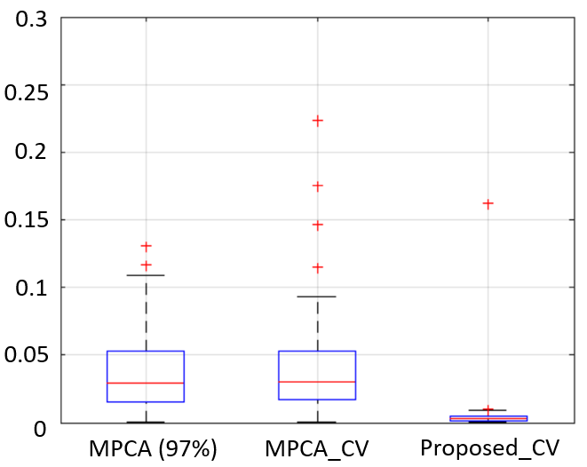


The Figures 4-6 also demonstrate that “MPCA_CV” always outperforms “MPCA (97%)”, and the superiority of “MPCA_CV” is augmented with the increase of data missing rate. For instance, when 10% images are missing, the median absolute prediction errors (and IQR) of “MPCA (97%)” and “MPCA_CV” are 0.058 (0.067) and 0.053 (0.063), respectively; when the missing rate is 50%, they are 0.302 (0.405) and 0.104 (0.168). One of the possible reasons is that “MPCA (97%)” determines the dimension of the tensor subspace by setting the “FVE” as 97%, which usually results in relatively high-dimensional features, although the dimension is smaller than that of the original image tensor. Relatively high-dimensional features implies an insufficient dimension reduction. In addition, it means the number of parameters in the subsequent LLS-based prognostic model is relatively large, which poses estimation challenges given that the number of samples (assets) for model training is limited.
6 Case Study
In this section, we use degradation image streams obtained from a rotating machinery test bed to validate the effectiveness of our proposed method. The test bed is designed to perform accelerated degradation tests on rolling entry thrust bearings. Specifically, bearings were run from brand new to failure. An FLIR T300 infrared camera was used to monitor the degradation process and collect degradation images over time. In the meanwhile, an accelerometer was mounted on the test bed to monitor the vibration of the bearing, and the failure time is defined as the time point where the amplitude of defective vibration frequencies crosses a threshold based on ISO standards for machine vibration. The data set consists of degradation image streams and their corresponding TTFs, and each image has pixels. As an illustration, a sequence of images obtained at different (ordered) time periods of one of the bearing are shown in Figure 7. More details about the experimental setup and the data set can be found in Gebraeel et al. 2009 and Fang et al. 2019.

We use 5-fold cross validation to evaluate the performance of our proposed model and the two benchmarks discussed in Section 5. Similar to the simulation study, we conduct 10-fold cross validation to determine the optimal weight parameter in criterion (4) and the most appropriate dimension of the tensor subspace. In addition, we also consider four levels of data incompleteness: (1) missing (i.e., complete), (2) missing, (3) missing, and (4) missing. Figure 9 illustrates the absolute prediction errors when degradation image streams are complete. Figure 9 shows prediction errors when 10% of the images of each bearing are missing. Figures 11 and 11 demonstrate the absolute prediction errors when the missing rate are 50% and 90%, respectively.
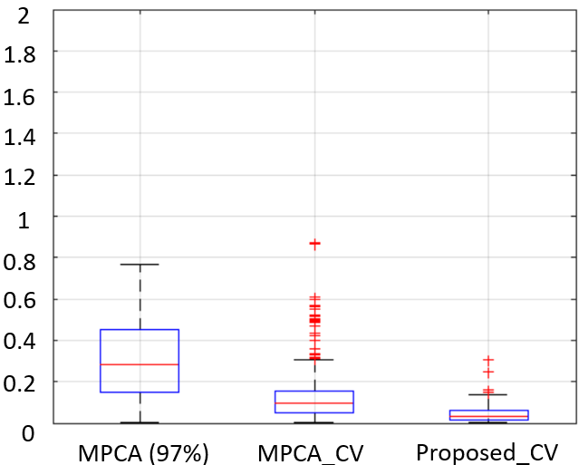


Similar to the discovery in the numerical study in Section 5, Figures 9, 9, 11, and 11 indicate that our proposed method constantly works better than the two benchmarks under all the 4 data missing rates. For example, the median absolute prediction errors (and IQRs) of our proposed method and the two benchmarks are 0.03 (0.04), 0.3 (0.24), and 0.1 (0.16), respectively, when the degradation image streams are complete. When 50% of the images are missing, the median absolute prediction errors (and IQR) of are respectively 0.09 (0.17), 0.62 (0.65), and 0.15 (0.19). We believe this is because our proposed model is a supervised dimension reduction-based method, which uses TTF information to supervise the defection of the low-dimensional tensor subspace, while the benchmarks are unsupervised dimension reduction-based methods without TTF information involved. Since our method considers TTF information when detecting the tensor subspace, the extracted features are more effective for failure time prediction.
Figure 9, 9, 11, 11 also show that the prediction errors of all the 3 methods increase with the increase of data missing rates. For example, when the missing rates are 0%, 10%, 50%, and 90%, the median absolute prediction errors (and IQRs) of “MPCA (97%)” are 0.3 (0.24), 0.49 (0.42), 0.62 (0.65), and 0.83 (0.78), respectively, while they are respectively 0.09 (0.11), 0.1 (0.16), 0.15 (0.19), and 0.31 (0.22) for “MPCA_CV”, and 0.03 (0.04), 0.05 (0.08), 0.09 (0.17), and 0.29 (0.21) for our proposed method. This is reasonable since a higher data missing rate means less useful degradation information and thus a worse model performance. In addition, we observe that the superiority of our proposed method over the two benchmarks decrease with the increase of data missing rates. For example, the prediction accuracy of our method and “MPCA (97%)” are comparable when the data missing rate is 90%. We again believe this is because not much useful information is available when data is highly incomplete and none of the two models perform well with such limited data.
We also observe that “MPCA_CV” always outperforms “MPCA (97%)”, and the superiority of “MPCA_CV” is augmented with the increase of data missing rate. For example, when 10% images are missing, the median absolute prediction errors (and IQR) of “MPCA (97%)” and MPCA_CV are 0.49 (0.42) and 0.1 (0.16), respectively; when the missing rate is 50%, the they are 0.62 (0.65) and 0.15 (0.19). We again believe this is because “MPCA (97%)” determines the dimension of the tensor subspace by setting the “FVE” as 97%, which results in relatively high-dimensional features due to the insufficient dimension reduction. Also, it results in a parameter estimation challenge since the number of parameters to be estimated in the prognostic model is relatively large comparing to the limited number of historical samples for model training. This suggests that cross validation is a better method to determine the dimension of the tensor subspace, especially when we do not have enough number of samples for model training.
7 Conclusions
This paper proposed a supervised tensor dimension reduction-based prognostic model for applications with incomplete degradation imaging data. This is achieved by first developing a new supervised tensor dimension reduction method that reduces the dimension of incomplete high-dimensional degradation image streams and provides low-dimensional tensor features, which are then used to build a prognostic model based on (log)-location-scale regression.
The supervised tensor dimension reduction method uses historical TTFs to supervise the detection of a low-dimensional tensor subspace to reduce the dimension of incomplete high-dimensional image streams. Mathematically, it is formulated as an optimization criterion that combines a feature extraction term and a regression term. The feature extraction term focuses on identifying a tensor space to extract low-dimensional tensor features from high-dimensional image streams. The regression term regresses failure times against the features extracted by the first term using LLS regression. By jointly optimizing the two terms, it is expected to detect an appropriate tensor subspace such that the extracted features are effective for TTF prediction. To estimate the parameters of the supervised dimension reduction method, we developed a Block Updating Algorithm for applications where TTFs follow distributions in the (log)-location-scale family. The algorithm works by splitting the parameters into several blocks and cyclically optimizing one block of parameters while keeping other blocks fixed until convergence. In addition, we showed that if TTFs follow normal or lognormal distributions, there is a closed-form solution when optimizing each block of the parameters, no matter the imaging data is complete or incomplete.
Simulated data as well as a data set from rotating machinery were used to validate the effectiveness of our proposed method. The results showed that our proposed prognostic method consistently outperforms the unsupervised tensor reduction-based benchmarks under various data missing rates. This validated the benefits and importance of using failure time information to supervise the dimension reduction of high-dimensional degradation image streams when building prognostic models.
The proposed prognostic model assumes that the TTFs of assets in the training dataset are known. In many real-world applications, the historical failure times might be right censored. This is because a component might be replaced before failure, so the exact TTF is unknown, and we only know that it is larger than the replacement time. How to incorporate censored TTFs into the proposed method can be an interesting future research topic.
Appendix
1 Proof of Proposition 1
The original optimization problem is
which is equivalent to the following problem when data is complete:
which is convex. Thus, it can be solved by setting the derivatives to be zeros–that is , where . This implies . According to the communication law of tensor mode multiplication, we have . Thus, , where . Furthermore, we have due to the fact that and the property of tensor mode multiplication . By taking the derivative of the Frobenius norm, we have . Thus, , which gives that . Finally, we have .
2 Proof of Proposition 2
The original optimization problem is
which is equivalent to the following problem when data is complete:
which is convex. Therefore, it can be solved by setting the derivatives to be zeros–that is , where . This implies . According to the communication law of tensor mode multiplication, we have . Thus, , where . Furthermore, we have due to the fact that and the property of tensor mode multiplicaion . By taking the derivative of the Frobenius norm, we have . Thus, which gives that . Finally we have .
3 Proof of Proposition 3
The original optimization problem is
which is equivalent to the following problem when data is complete:
which is convex. Therefore, it can be solved by setting the derivatives to be zeros–that is , where . This implies . According to the communication law of tensor mode multiplication, we have . Thus, , where . Furthermore, we have due to the fact that and the property of tensor mode multiplicaion . By taking the derivative of the Frobenius norm, we have . Thus, , which gives that . Finally, we have .
4 Proof of Proposition 4
The original optimization problem is
which is equivalent to the following problem when data is complete:
which is convex. Thus, it can be solved by setting the derivatives to be zeros–that is , where . According to the connection between Kronecker product and tensor mode multiplication (Kolda 2006), we have . By taking the derivative of the Frobenius norm, we have . Thus, . Finally, we have .
5 Proof of Lemma 1
Let denotes the th row of matrix and denotes the th row of matrix , , then we have
Based on the definition of Frobenius norm, the original objective function in Lemma 1 can be transformed as follows:
Therefore, we have the following:
where . Therefore, to solve the original objective function, we can simply solve the following sub problems:
6 Proof of Proposition 5
The original optimization problem is
which is equivalent to the following problem when data is missing:
where is the inner product, logic() denotes the logical value of –that is–if an entry is observed, its logical value is 1; otherwise, it is 0. Since the problem is convex, it can be solved by setting the derivatives to be zeros, i.e., , where . This implies . According to the communication law of tensor mode multiplication, we have . Thus, , where . Furthermore, we have since and .
Figure 12 shows the pattern of mode-1 matricization of the 4D tensor when it has missing entries whose indices can be denoted by a set . Based on Lemma 1, we can sequentially optimize each column of .

Specifically, we denote the th row in as (blue solid row of in Figure 12). The available entries in the th row of are denoted as (blue striped squares of in Figure 12). In , we choose the columns whose indices are the same as those of the available entries of (blue striped columns of in Figure 12). As a result, we have . Because we only take the derivative of , we have . By taking the derivative of the Frobenius norm, we have . Thus, , which gives that .
7 Proof of Proposition 6
The original optimization problem is
which is equivalent to the following problem when data is incomplete:
where is the inner product, logic() denotes the logical value of . Since the problem is convex, it can be solved by setting the derivatives to be zeros, i.e., , where . This implies . According to the communication law of tensor mode multiplication, we have . Thus, , where . Furthermore, we have due to the fact that and (a property of tensor mode multiplication).

As discussed earlier, for applications with missing images, the indices of tensor ’s missing entries can be denoted as , , where “” denotes all the indices in a dimension. As a result, it can be easily shown that ’s mode-1 matricization has missing columns (see Figure 13 for an illustration). Let be the set consisting of the indices of available columns in , then we need to solve , where denotes a matrix constituting the columns of . Thus, we have . Thus, , which gives that . This yields the solution .
8 Proof of Proposition 7
The original optimization problem is
which is equivalent to the following problem when data is missing:
where is the inner product, logic() denotes the logical value of . Since the problem is convex, it can be solved by setting the derivatives to be zeros, i.e., , where . This implies . According to the communication law of tensor mode multiplication, we have . Thus, , where . Furthermore, we have since and .

Figure 14 shows the pattern of mode-2 matricization of the 4D tensor when it has missing entries whose indices can be denoted by a set . Based on Lemma 1, we can sequentially optimize each column of .
Specifically, we denote the th row in as (blue solid row of in Figure 14). The available entries in the th row of are denoted as (blue striped squares of in Figure 14). In , we choose the columns whose indices are the same as those of the available entries in (blue striped columns of in Figure 14). As a result, we have . Since on the derivative of is taken, we have . By taking the derivative of the Frobenius norm, we have . Thus, , which gives that .
9 Proof of Proposition 8
The original optimization problem is
which is equivalent to the following problem when data is incomplete:
where is the inner product, logic() denotes the logical value of . Since the optimization criterion is convex, it can be solved by setting the derivatives to be zeros, i.e., , where . This implies . According to the communication law of tensor mode multiplication, we have . As a result, , where . Furthermore, we have since and .

It can be easily shown that ’s mode-2 matricization has missing columns as well (see Figure 15 for an illustration). Therefore, similar to the proof of Proposition 9, we have , where denotes the indices of available columns in , denotes a matrix constituting the columns of . As a result, we have . Thus, , which gives that . This yields the analytical solution .
10 Proof of Proposition 9
The original optimization problem is
which is equivalent to the following problem when data is missing:
where is the inner product, logic() denotes the logical value of . Since the problem is convex, it can be solved by setting the derivatives to be zeros, i.e., , where . This implies . According to the communication law of tensor mode multiplication, we have . Thus, , where . Furthermore, we have since and .

Figure 16 shows the pattern of mode-3 matricization of the 4D tensor when it has missing entries whose indices can be denoted by a set . Based on Lemma 1, we can sequentially optimize each column of . The th row in is denoted as (blue solid row of in Figure 16). The available entries in the th row of are denoted as (blue striped squares of in Figure 16). In , we choose the columns whose indices are the same as those of the available entries of (blue striped columns of in Figure 16). Thus, we have , which yields . By taking the derivative of the Frobenius norm, we have . Thus, , which gives that .
11 Proof of Proposition 10
The original optimization problem is
which is equivalent to the following problem when data is missing:
where is the inner product, logic() denotes the logical value of . Since the problem is convex, it can be solved by setting the derivative to be zeros–that is , where . According to the connection between Kronecker product and tensor mode multiplication, we have .

Figure 17 shows the pattern of mode-4 matricization of the 4D tensor when it has missing entries whose indices can be denoted by a set . Based on Lemma 1, we can sequentially optimize each column of .
The th row in is denoted as (blue solid row of in Figure 17). The available entries in the th row of are denoted as (blue striped squares of in Figure 17). In , we choose the columns whose indices are the same as those of the available entries of (blue striped columns of in Figure 17). Thus, we have , which yields . By taking the derivative of Frobenius norm, we have . Thus, , which gives that .
References
- Abdi and Williams (2010) Abdi, H. and L. J. Williams (2010). Principal component analysis. Wiley interdisciplinary reviews: computational statistics 2(4), 433–459.
- Aydemir and Paynabar (2019) Aydemir, G. and K. Paynabar (2019). Image-based prognostics using deep learning approach. IEEE Transactions on Industrial Informatics 16(9), 5956–5964.
- Bogdanoff and Kozin (1985) Bogdanoff, J. L. and F. Kozin (1985). Probabilistic models of cumulative damage(book). New York, Wiley-Interscience, 1985, 350 p.
- Dong et al. (2021) Dong, Y., T. Xia, D. Wang, X. Fang, and L. Xi (2021). Infrared image stream based regressors for contactless machine prognostics. Mechanical Systems and Signal Processing 154, 107592.
- Doray (1994) Doray, L. (1994). Ibnr reserve under a loglinear location-scale regression model. In Casualty Actuarial Society Forum, Volume 2, pp. 607–652. Citeseer.
- Fang et al. (2019) Fang, X., K. Paynabar, and N. Gebraeel (2019). Image-based prognostics using penalized tensor regression. Technometrics 61(3), 369–384.
- Filipović and Jukić (2015) Filipović, M. and A. Jukić (2015). Tucker factorization with missing data with application to low-n-rank tensor completion. Multidimensional systems and signal processing 26(3), 677–692.
- Gebraeel et al. (2009) Gebraeel, N., A. Elwany, and J. Pan (2009). Residual life predictions in the absence of prior degradation knowledge. IEEE Transactions on Reliability 58(1), 106–117.
- Gebraeel et al. (2005) Gebraeel, N. Z., M. A. Lawley, R. Li, and J. K. Ryan (2005). Residual-life distributions from component degradation signals: A bayesian approach. IiE Transactions 37(6), 543–557.
- Hastie et al. (2009) Hastie, T., R. Tibshirani, and J. Friedman (2009). The elements of statistical learnin. Cited on 33.
- Hong and Meeker (2010) Hong, Y. and W. Q. Meeker (2010). Field-failure and warranty prediction based on auxiliary use-rate information. Technometrics 52(2), 148–159.
- Hong and Meeker (2013) Hong, Y. and W. Q. Meeker (2013). Field-failure predictions based on failure-time data with dynamic covariate information. Technometrics 55(2), 135–149.
- Jiang et al. (2023) Jiang, Y., T. Xia, X. Fang, D. Wang, E. Pan, and L. Xi (2023). Sparse hierarchical parallel residual networks ensemble for infrared image stream-based remaining useful life prediction. IEEE Transactions on Industrial Informatics.
- Jiang et al. (2022a) Jiang, Y., T. Xia, D. Wang, X. Fang, and L. Xi (2022a). Adversarial regressive domain adaptation framework for infrared thermography-based unsupervised remaining useful life prediction. IEEE Transactions on Industrial Informatics.
- Jiang et al. (2022b) Jiang, Y., T. Xia, D. Wang, X. Fang, and L. Xi (2022b). Spatiotemporal denoising wavelet network for infrared thermography-based machine prognostics integrating ensemble uncertainty. Mechanical Systems and Signal Processing 173, 109014.
- Kolda (2006) Kolda, T. G. (2006). Multilinear operators for higher-order decompositions. Technical report, Citeseer.
- Kolda and Bader (2009) Kolda, T. G. and B. W. Bader (2009). Tensor decompositions and applications. SIAM review 51(3), 455–500.
- Liu et al. (2012) Liu, J., P. Musialski, P. Wonka, and J. Ye (2012). Tensor completion for estimating missing values in visual data. IEEE transactions on pattern analysis and machine intelligence 35(1), 208–220.
- Liu et al. (2013) Liu, K., N. Z. Gebraeel, and J. Shi (2013). A data-level fusion model for developing composite health indices for degradation modeling and prognostic analysis. IEEE Transactions on Automation Science and Engineering 10(3), 652–664.
- Lu et al. (2008) Lu, H., K. N. Plataniotis, and A. N. Venetsanopoulos (2008). Mpca: Multilinear principal component analysis of tensor objects. IEEE transactions on Neural Networks 19(1), 18–39.
- Prautzsch et al. (2002) Prautzsch, H., W. Boehm, and M. Paluszny (2002). Bézier and B-spline techniques, Volume 6. Springer.
- Ramsay and Silverman (2005) Ramsay, J. and B. Silverman (2005). Principal components analysis for functional data. Functional data analysis, 147–172.
- Shu et al. (2015) Shu, Y., Q. Feng, and D. W. Coit (2015). Life distribution analysis based on l évy subordinators for degradation with random jumps. Naval Research Logistics (NRL) 62(6), 483–492.
- Wang et al. (2021) Wang, F., M. R. Gahrooei, Z. Zhong, T. Tang, and J. Shi (2021). An augmented regression model for tensors with missing values. IEEE Transactions on Automation Science and Engineering.
- Wang et al. (2022) Wang, F., A. Wang, T. Tang, and J. Shi (2022). Sgl-pca: Health index construction with sensor sparsity and temporal monotonicity for mixed high-dimensional signals. IEEE Transactions on Automation Science and Engineering.
- Xu et al. (2013) Xu, Y., R. Hao, W. Yin, and Z. Su (2013). Parallel matrix factorization for low-rank tensor completion. arXiv preprint arXiv:1312.1254.
- Xu and Yin (2013) Xu, Y. and W. Yin (2013). A block coordinate descent method for regularized multiconvex optimization with applications to nonnegative tensor factorization and completion. SIAM Journal on imaging sciences 6(3), 1758–1789.
- Yang et al. (2021) Yang, Z., P. Baraldi, and E. Zio (2021). A multi-branch deep neural network model for failure prognostics based on multimodal data. Journal of Manufacturing Systems 59, 42–50.
- Ye and Chen (2014) Ye, Z.-S. and N. Chen (2014). The inverse gaussian process as a degradation model. Technometrics 56(3), 302–311.
- Ye et al. (2014) Ye, Z.-S., M. Xie, L.-C. Tang, and N. Chen (2014). Semiparametric estimation of gamma processes for deteriorating products. Technometrics 56(4), 504–513.