Self-regulation of black hole accretion via jets in early protogalaxiesSelf-regulation of black hole accretion via jets in early protogalaxies–A2021
Abstract
The early growth of black holes in high-redshift galaxies is likely regulated by their feedback on the surrounding gas. While radiative feedback has been extensively studied, the role of mechanical feedback has received comparatively less scrutiny to date. Here we use high-resolution parsec-scale hydrodynamical simulations to study jet propagation and its effect on black hole accretion onto 100 black holes in the dense, low-metallicity gas expected in early protogalaxies. As the jet propagates, it shocks the surrounding gas and forms a jet cocoon. The cocoon consists of a rapidly-cooling cold phase at the interface with the background gas and an over-pressured subsonic phase of reverse shock-heated gas filling the cocoon interior. We systematically vary the background gas density and temperature, black hole feedback efficiency, and the jet model. We found that the width of the jet cocoon roughly follows a scaling derived by assuming momentum conservation in the jet propagation direction, and energy conservation in the lateral directions. Depending on the assumed gas and jet properties, the cocoon can either stay elongated out to a large radius or isotropize before reaching the Bondi radius, forming a nearly spherical bubble. Lower jet velocities and higher background gas densities result in self-regulation to higher momentum fluxes and elongated cocoons. In all cases, the outward momentum flux of the cocoon balances the inward momentum flux of the inflowing gas near the Bondi radius, which ultimately regulates black hole accretion.We also examine the accretion variability and find that the larger the distance the jet cocoon reaches (either due to lower temperature or a more elongated jet cocoon), the longer the variability timescale of the black hole accretion rate. Overall, we find that the time-averaged accretion rate always remains below the Bondi rate, and exceeds the Eddington rate only if the ambient medium is dense and cold, and/or the jet is weak (low velocity and mass-loading). We derive the combination of jet and ambient gas parameters yielding super-Eddington growth.
Keywords:
methods: numerical — galaxies: jets — accretion, accretion discs — black hole physics — hydrodynamics1 Introduction
The origin of supermassive black holes (SMBHs) with masses of , powering bright quasars observed in the first billion years after the Big Bang (redshifts ; see, e.g. Bosman 2022 for an up-to-date compilation) remains an unsolved puzzle. Proposed explanations range from rapid, super-Eddington growth of stellar mass seed black holes (BHs), the “direct collapse” of a supermassive star, to runaway mergers between stellar-mass objects, as well as more exotic phenomena (see, e.g. Inayoshi et al. 2020; Volonteri et al. 2021, for recent comprehensive reviews).
One promising scenario is for a low-mass seed BH to grow at rates well above the fiducial Eddington rate (where is the Eddington luminosity, is the speed of light, and is a radiative efficiency). Indeed, small-scale simulations of BH accretion show that BHs surrounded by dense gas can accrete at rates up to at least (Jiang et al. 2014; Sadowski et al. 2014, e.g.,). However, feedback from the BH accretion itself poses possible obstacles to sustaining such rapid growth. Even in the presence of dense ambient gas, allowing rapid fueling, radiative feedback on large scales tends to make the accretion episodic, with a strongly suppressed time-averaged accreton rate (Milosavljević et al. 2009; Park & Ricotti 2011, e.g.). BH radiation may also outright eject gas from the shallow gravitational potential of its low-mass parent halo, preventing rapid accretion (Alvarez et al. 2009a). On the other hand, these deleterious radiative effects may be avoided in the hyper-Eddington regime, in which radiation is trapped and cannot exert large-scale feedback (Inayoshi et al. 2016; Takeo et al. 2020).
In addition to radiative feedback, mechanical feedback presents another potential obstacle to rapid and sustained BH growth. While such mechanical feedback has been less explored in the high-redshift context, it is well established to play a crucial role in galaxy formation and evolution at lower redshifts. Active galactic nucleus (AGN) feedback is known to quench star-formation in massive galaxies and clusters, keeping them “red and dead” over a significant fraction of cosmic time. Among the different forms of AGN feedback, extensive galaxy-scale simulations have shown that AGN jet models are, in principle, capable of quenching a galaxy and stopping the cooling flows (Dubois et al. 2010; Gaspari et al. 2012; Yang et al. 2012; Li & Bryan 2014; Li et al. 2015; Prasad et al. 2015; Yang & Reynolds 2016; Ruszkowski et al. 2017; Bourne & Sijacki 2017; Martizzi et al. 2019; Su et al. 2020, e.g.,). Observational studies also infer that AGN can provide an energy budget comparable to the cooling rate (Bîrzan et al. 2004). There are also observations of unambiguous cases of AGN expelling gas from galaxies, injecting thermal energy via shocks or sound waves, via photo-ionization and Compton heating, or via “stirring” the circum-galactic medium (CGM) and intra-cluster medium (ICM). This can create “bubbles” of hot plasma with non-negligible relativistic components, which are ubiquitous around massive galaxies (see, e.g., Fabian 2012; Hickox & Alexander 2018, for a detailed review). In Su et al. 2021 and Su et al. (in prep.), we carried out a broad parameter study of AGN jets in clusters and found a subset of models which inflate a sufficiently large cocoon with a long enough cooling time that these jets can quench the central galaxy.
In addition to the thoroughly studied cases of SMBHs in massive galaxies, various studies also suggested AGN feedback in much smaller dwarf galaxies and from intermediate-mass black holes (; Nyland et al. 2017; Bradford et al. 2018; Penny et al. 2018; Dickey et al. 2019; Manzano-King et al. 2019), some of which are observed in the form of AGN jets (Greene et al. 2006; Wrobel & Ho 2006; Wrobel et al. 2008; Mezcua & Lobanov 2011; Nyland et al. 2012; Reines & Deller 2012; Webb et al. 2012; Mezcua et al. 2013a; Mezcua et al. 2013b; Reines et al. 2014; Mezcua et al. 2015; Mezcua et al. 2018a; Mezcua et al. 2018b; Mezcua et al. 2019, e.g.,). Unsurprisingly, AGN feedback can also affect the growth of these smaller black holes, alter the surrounding gas properties, and play a significant role in sculping the galaxy they live in, especially in dwarfs and high-redshift galaxies (Wellons et al. 2022).
Observations also find supermassive black holes () at high-redshift () with jetted AGN quasars (Sbarrato et al. 2021; Sbarrato et al. 2022, e.g.,). It is unclear whether a 100 black hole, which can be presumed to produce jets, as well, if it is fed at super-Eddington rates, could sustain rapid growth onto a supermassive black hole. Recent work has addressed this problem in slightly different contexts, either investigating the impact of wider-angle outflows produced at larger radii in the accretion flow (Takeo et al. 2020, e.g.,), or by utilizing galaxy-scale simulations to assess the growth of larger black holes () with a jet (Regan et al. 2019; Massonneau et al. 2022, e.g.,). The present work aims to study how AGN jets affect accretion onto “seed” black holes in dense, low-metallicity gas, mimicking conditions expected in high-redshift protogalaxies. Additionally, we study in detail the physics of how jet-inflated cocoons propagate to large radii and self-regulate BH accretion, using analytic models to interpret our simulation results.
In galaxy-scale simulations, including in our own previous work (Torrey et al. 2020; Su et al. 2020; Su et al. 2021; Wellons et al. 2022, e.g,), both AGN feedback and BH accretion have been implemented with sub-grid prescriptions. Models based on Bondi-Hoyle accretion (Bondi 1952; Springel et al. 2005) and accretion via gravitational torques (Hopkins & Quataert 2011; Anglés-Alcázar et al. 2017) involve assumptions about gas properties, which might not always be valid, especially in the presence of an unresolved jet. To better address this question, in this work, we model a cloud of gas with systematically varied properties around the black hole at sufficiently high resolution (with the minimum gravitational force softening at least 1000 times less than the Bondi radius), to resolve the gravitational capture of individual gas particles (Hopkins et al. 2016; Anglés-Alcázar et al. 2021). We also implement various jet models to study how they affect BH accretion and how the jet propagates to a larger radius. Although the jets in this study are launched at a much smaller scale, the initial jet itself remains sub-grid relative to the scales we can resolve. This work also addresses how sub-grid jet models launched on different scales connect to each other. We also parameterize the results of our simulations in order to provide the effective long-term time-averaged accretion rate, given different gas properties beyond the Bondi radius and with different jet models. . We delineate the parameter space of gas and jet properties over which super-Eddington growth may occur.
The rest of this paper is organised as follows. In § 2, we summarise our initial conditions (ICs), black hole accretion model and the AGN jet parameters we survey, and we describe our numerical simulations. We present the results with different jet velocities, which show the most dramatic differences, in § 3. We develop a toy model describing the regulation of different jet models in different environments in § 4. We present a suite of additional simulations with varying model parameters and compare the results with the toy model in § 5. We compare our study to several other recent works, and summarise the implications of our findings in § 6. We enumerate our main conclusions in § 7. We include a set of simulations exploring numerical choices, as well as resolution studies, in Appendix A.
2 Methodology
We perform simulations of a box of gas under the effect of jet feedback from a 100 black hole. Our simulations use GIZMO11 1 A public version of this code is available at http://www.tapir.caltech.edu/phopkins/Site/GIZMO.html (Hopkins 2015), in its meshless finite mass (MFM) mode, which is a Lagrangian mesh-free Godunov method, capturing advantages of both grid-based and smoothed-particle hydrodynamics (SPH) methods. Numerical implementation details and extensive tests are presented in a series of methods papers for, e.g., hydrodynamics and self-gravity (Hopkins 2015). All of our simulations employ the FIRE-2 implementation of cooling (followed from K), including the effects of photo-electric and photo-ionization heating, collisional, Compton, fine-structure, recombination, atomic, and molecular cooling (Hopkins et al. 2018, following). Note that we impose a temperature floor at , which will be specified in the initial conditions (and systematically varied), assuming other feedback processes not included in these simulations keep the gas from cooling further. We assume a metallicity of , which may be expected in the protogalaxies hosting the first stellar-mass BH seeds, and which is sufficiently low that metal cooling above K (the lowest value of that we adopt) is negligible.
2.1 Initial conditions
Ideally, we would evolve the black hole accretion within the context of a cosmological simulation that resolves the gas dynamics at high redshift (Alvarez et al. 2009b, e.g., as done for minihalos by). However, given the very large uncertainties in high-redshift conditions, we instead approximate the physical conditions near the black hole as a uniform patch of gas. This allows us to systematically vary the gas properties in order to understand how these impact the black hole regulation. In particular, the initial condition we adopt is a uniform 3D-box of uniformly-distributed gas particles with constant density and temperature, which we denote and . A 100 black hole is placed at the center of the box. As mentioned above, the initial metallicity of the gas is set to a very low value ( ).
To achieve a higher resolution in the vicinity of the black hole, where the accretion occurs and the overall regulation is determined, and in the vicinity of the jet, we use a hierarchical super-Lagrangian refinement scheme (Su et al. 2020; Su et al. 2021) to reach mass resolution around the z-axis where the jet is launched, much higher than many previous global studies (Weinberger et al. 2017; Su et al. 2021, e.g.,). The mass resolution decreases as a function of distance from the z-axis (), roughly proportional to for pc. The numerical details are summarized in Table 1. The highest resolution region is where is smaller than pc unless otherwise stated. A resolution study is presented in Appendix A.
2.2 BH accretion
As discussed in the introduction, black hole accretion is not modelled with the Bondi assumption, but instead is determined by following the gravitational capture of gas (Hopkins et al. 2016; Anglés-Alcázar et al. 2021) directly, and implementing its subsequent accretion onto the black hole via an -disk prescription (see below). A gas particle is accreted if it is gravitationally bound to the black hole and the estimated apocentric radius is smaller than 22 2 This provides a scale for the sub-grid accretion model and for the -disk model.. This sink radius is set to pc according to the black hole neighborhood gas density. In more detail, the sink radius is set to be a radius from the black hole enclosing 96 “weighted” neighborhood gas particles but capped to be within ( pc).
Although we follow the gas down to distances very close to the black hole, we do not model the accretion disk itself, but instead adopt a simple -disk model. The accreted gas adds to the -disk mass (, which is initially set to zero). The mass in the -disk is then supplied to the black hole at the rate
| (1) |
We assume a constant year from an estimated viscous time scale of a Shakura & Sunyaev 1973 disk, assuming the accretion disk is at , as , where is the free fall time at and is the Mach number of gas in the -disk. In Appendix A we explore the impact of varying .
2.3 Jet models
We adopt a jet model following Su et al. 2021. In brief, a jet is launched with a particle-spawning method, which creates new gas cells (”resolution elements”) to represent the jet material. The spawned particles have a fixed initial mass, temperature, and velocity, which sets the specific energy of the jet. With this method we have better control of the jet properties, as launching using particle spawning depends less on local gas properties than when depositing energy/momentum based on the distribution of neighboring gas elements 33 3 The traditional method usually does a particle neighbor search from the black hole and dumps the designated energy and momentum into these gas particles. Therefore, the effect will depend on the local gas properties and the exact geometric distribution. See Wellons et al. 2022 for a comparison of different methods.. We can also enforce a higher resolution for the jet elements, allowing light jets to be accurately modeled. The spawned gas particles have a mass resolution as indicated in Table 1 and are forbidden to de-refine (merge into a common gas element) before they decelerate to 10% of the launch velocity. Two particles are spawned in opposite z-directions at the same time when the accumulated jet mass flux reaches twice the target spawned particle mass, so linear momentum is always exactly conserved. Initially, the spawned particle is randomly placed on a sphere with a radius of , which is either pc or half the distance between the black hole and the closest gas particle, whichever is smaller. If the particle is initialized at a position in spherical polar coordinates, and the jet opening-angle of a specific model is (say , which is the case for our jet model), the polar angle of the initial velocity direction of the jet will be set at .With this, the projected paths of any two particles will not intersect.
We parameterize the jet mass flux with a constant feedback mass fraction
| (2) |
so the feedback energy and momentum fluxes are
| (3) |
where is the adopted jet velocity and is the mean particle mass.
| Numerical details | Feedback parameters | Background gas | Resulting averaged accretion rate and fluxes | ||||||||||
| Model | Box size | ||||||||||||
| kyr | pc | km s-1 | K | cm-3 | K | ||||||||
| Fiducial | |||||||||||||
| 5e-2–j1e4–n1e5–T1e4 (I,II,III)∗ | 100 | 0.4 | 1.4e-6 | 1e-7 | 0.05 | 1e4 | 1e4 | 1e5 | 6e3 | 0.7-1.5e-7 | 2.1-4.6e-3 | 0.031-0.067 | 0.87-1.9e-5 |
| Feedback mass fraction | |||||||||||||
| 5e-3–j1e5–n1e5–T1e4 | 100 | 0.4 | 1.4e-6 | 1e-7 | 0.005 | 1e4 | 1e4 | 1e5 | 6e3 | 9.4e-7 | 2.9e-2 | 0.42 | 1.2e-5 |
| 5e-1–j1e5–n1e5–T1e4 | 100 | 0.4 | 1.4e-6 | 1e-7 | 0.5 | 1e4 | 1e4 | 1e5 | 6e3 | 1.3e-8 | 4e-4 | 5.8e-3 | 1.6e-5 |
| Jet velocity | |||||||||||||
| 5e-2–j3e3–n1e5–T1e4 | 90 | 0.8 | 1.4e-6 | 1e-7 | 0.05 | 3e3 | 1e4 | 1e5 | 6e3 | 1e-5 | 0.31 | 4.5 | 1.1e-4 |
| 5e-2–j3e4–n1e5–T1e4 | 100 | 0.4 | 1.4e-6 | 1e-7 | 0.05 | 3e4 | 1e4 | 1e5 | 6e3 | 8.9e-9 | 2.7e-4 | 4.0e-3 | 1e-5 |
| Thermal jet | |||||||||||||
| 5e-2–Tj3e9–n1e5–T1e4 | 100 | 0.4 | 1.4e-6 | 1e-7 | 0.05 | 1e4 | 3e9 | 1e5 | 6e3 | 2.4e-8 | 7.4e-4 | 0.011 | 3.0e-6 |
| Gas density | |||||||||||||
| 5e-2–j3e3–n1e2–T1e4 | 100 | 0.4 | 1.4e-9 | 1e-10 | 0.05 | 1e4 | 1e4 | 1e2 | 6e3 | 1.6e-11 | 4.9e-4 | 7.2e-6 | 2e-9 |
| 5e-2–j3e3–n1e3–T1e4 | 100 | 0.4 | 1.4e-8 | 1e-9 | 0.05 | 1e4 | 1e4 | 1e3 | 6e3 | 2.3e-10 | 7.0e-4 | 1.0e-4 | 2.9e-8 |
| 5e-2–j3e3–n1e4–T1e4 | 100 | 0.4 | 1.4e-7 | 1e-8 | 0.05 | 1e4 | 1e4 | 1e4 | 6e3 | 3.5e-9 | 1.1e-3 | 1.6e-3 | 4.4e-7 |
| 5e-2–j3e3–n1e6–T1e4 | 40 | 0.8 | 1.4e-5 | 1e-6 | 0.05 | 1e4 | 1e4 | 1e6 | 6e3 | 1.3e-5 | 4e-2 | 5.8 | 1.6e-3 |
| Gas temperature | |||||||||||||
| 5e-2–j3e3–n1e5–T1e3 | 50 | 3.2 | 1.4e-6 | 1e-7 | 0.05 | 1e4 | 1e4 | 1e4 | 6e3 | 1.9e-6 | 4.2e-3 | 0.85 | 2.4e-4 |
| 5e-2–j3e3–n1e5–T1e5 | 12 | 0.08 | 1e-8 | 8e-10 | 0.05 | 1e4 | 1e4 | 1e4 | 1e5 | 4.4e-9 | 2.9e-2 | 2.0e-3 | 5.5e-7 |
This is a partial list of simulations studied here with different jet and background gas parameters. The columns list:
(1) Model name: The naming of each model starts with the feedback mass fraction, followed by the jet velocity in km s-1 for kinetic jet or jet temperature in K for thermal dominant jet. The final 2 numbers labels the background gas density in cm-3 and background gas temperature in K.
(2) : Simulation duration (all shorter than the free-fall time for constant gas without a BH).
(3) Box size of the simulation.
(4) : The highest mass resolution.
(5) : The mass resolution of the spawned jet particles.
(6) : The feedback mass fraction.
(7) : The initial jet velocity at spawn.
(8) : The initial jet temperature at spawn.
(9) : The background gas density.
(10) : The background gas temperature.
(11) : The resulting time-averaged accretion rate.
(12) : The same value over Bondi accretion rate.
(13) : The same value over the Eddington accretion rate ().
(14) : Jet energy flux over Eddington luminosity.
∗ We run three variations of the same run with different random seeds for the stochastic injection of jet particles
(labeled as I, II, III) to characterize the impact of this stochasticity. Unless specified otherwise, in the rest of this paper we refer to run I.
3 Two modes of jet propagation
Before exploring all of the simulations that we have run, we first focus on a set of three simulations all with the same fiducial background gas properties ( and K) and feedback mass fraction (), but varying the jet velocity, ranging from 3000 - 30000 km s-1. These models are denoted as “5e-2–j3e3–n1e5–T1e4”, “5e-2–j1e4–n1e5–T1e4” (I,II,III), and “5e-1–j3e4–n1e5–T1e4”. These velocity variations result in very different jet cocoons and, as we will see, guide our development of a simple model which will explain how the jet evolves when we modify other parameters (such as the background gas properties).
3.1 Cocoon morphology
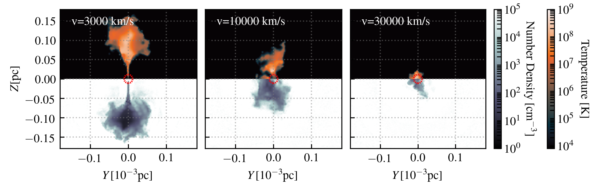
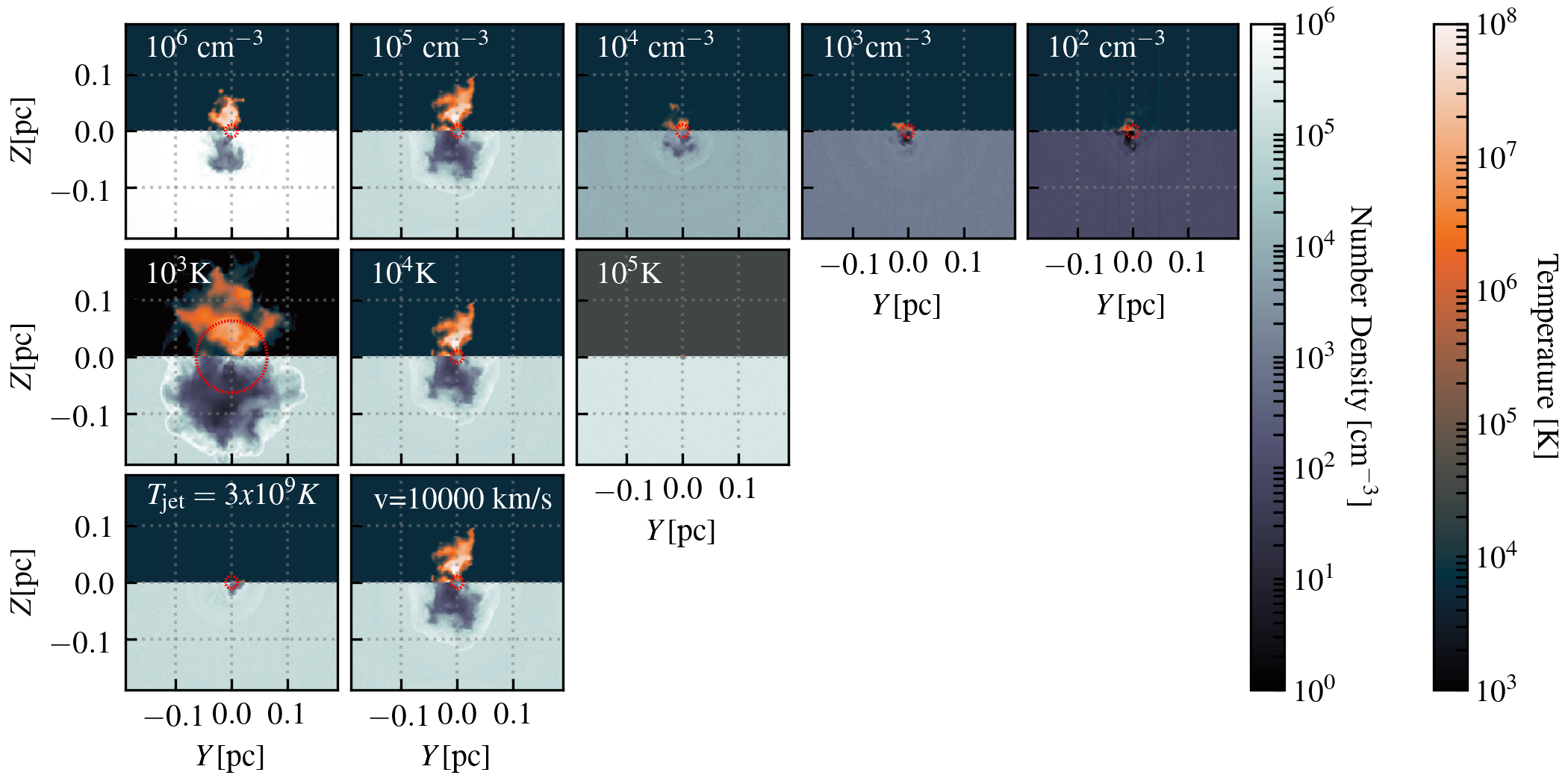
Fig. 1 shows the morphology of the cocoon for the three different jet velocities, depicting the resulting density and temperature distributions. Note that, in these figures, the hot jet gas is most clearly visible, but this is surrounded by a region of shocked ambient material. We use the term “cocoon” to refer to the combination of both regions. The black hole accretion and resulting jet are highly episodic (see Fig. 2), and as a result, the length and the width of the jet cocoon are also time-dependent. We choose a snapshot where each cocoon reaches its maximum height in order to show the differences most clearly. This figure shows that the propagation of the jet cocoon varies primarily in length. The run with a lower jet velocity has a much more elongated jet cocoon, reaching a much larger distance. On the other hand, the higher velocity runs result in a roughly isotropic bubble-shaped cocoon. The higher the velocity, the shorter the distance the jet cocoon reaches.
Qualitatively, this is primarily because a lower velocity jet with lower specific energy regulates itself to a higher mass and momentum flux (for reasons we will discuss below). The higher mass and momentum flux jet can punch through to a much larger radius, consistent with what we see in galaxy scale jet simulations (e.g., Krause 2003, Guo 2015, Su et al. 2021 and Weinberger et al. in prep.). We will provide a more quantitative scaling for the propagation of the jet cocoon with jet models and the initial external gas density and temperature in § 4.
3.2 BH Accretion Rate and Jet energy Flux
Fig. 2 shows the resulting black hole accretion rate, jet mass flux, momentum flux and energy flux as a function of time for the same set of runs. The latter quantity is the cumulative-average from the beginning of the run to the given time to reduce the noise. With a feedback mass fraction of , the black hole accretion rate roughly regulates to , , and for jet velocities of 3000, 10000, and 30000 km/s, respectively. We also see that the higher the jet velocity, the more short-term variability there is throughout the simulations, a topic we will return to in § 5.5.
Consistent with what we saw in § 3.1, a low-velocity jet regulates to a much higher mass and momentum flux, which is responsible for the more elongated cocoon. The 10000 and 30000 km s-1 runs, both of which have cocoons that isotropize at small radius, roughly regulate to a similar jet energy flux, meaning that with . The lowest velocity run (3000 km s-1), on the other hand, results in an even higher energy flux, qualitatively consistent with the much larger volume of the cocoon we see in Fig. 1. The lower velocity runs ( km s-1) roughly have , with . We will explore the reason behind the different behaviour and scalings of the high and low velocity jets in the next section.
4 A simple model for jet propagation and cocoon formation
In the previous section, we found that when we varied the jet velocity, the jets all self-regulated, but this could result either in a nearly spherical, or in a highly elongated cocoon. Here we develop a simple analytic model based on this dichotomy and then, in the next section, we will use it to understand self-regulation when other parameters, such as the background gas properties, are changed.
4.1 Jet propagation

We begin by reviewing the scaling which controls the cocoon shape before, in the next section, connecting this back to the accretion and hence overall self-regulation.
4.1.1 Elongated jet cocoon – before the cocoon isotropizes
We start by assuming the jet cocoon roughly follows a cylindrical geometry. As shown in Fig. 3, closer to where jets are launched, the propagation of the jet qualitatively follows from momentum conservation in the z-direction (Begelman & Cioffi 1989; Su et al. 2021, e.g.,),
| (4) |
where is the cross section of the pressurized cylinder (cocoon), is the expansion velocity of the cocoon in the polar directions, is the jet’s initial mass flux, and is the initial jet velocity.
The evolution in the perpendicular direction is, instead, dictated by energy conservation, as the build-up of an over-pressured cocoon drives lateral expansion. The resulting expansion then pushes the surrounding gas. The equations describing the conservation of energy and momentum flux can be written as
| (5) |
, where is the lateral surface area of the same region, is the height to which the jet reaches, is the immediate post shock velocity of the hot cocoon gas, is the expansion velocity of the cocoon in the mid-plane direction, is an order-of-unity geometric factor for the surface area of the cocoon with respect to an ideal cylindrical geometry, and is the ratio of the energy flux in the perpendicular direction (proportional to the total injected energy ) to the injected kinetic energy flux. Energy conservation is appropriate for the (initial) lateral expansion despite the strong cooling that can occur at the interface between the hot and cold gas within the cocoon. The total amount of cooling at this interface is proportional to its area (i.e. ) and so is negligible compared with the jet energy flux at early times.
In this expression, is the cocoon gas density, which we will assume depends on the jet velocity and the background gas properties as:
| (6) |
where , , and are exponents that we will determine later. Assuming the cocoon is pressurized by strong shocks (where and ), is roughly
| (7) |
Therefore, we assume is a constant for the remainder of the paper.
From the equations above, we can solve for the time dependence of and as
| (8) |
and the time dependence of and as
| (9) |
In particular, the opening angle of the resulting cocoon scales as
| (10) |
We have assumed that the jet starts such that , but as the cocoon propagates, for a fixed , eventually, it becomes (quasi-)isotropic (); this occurs at a time given by
| (11) |
and at a cocoon height of (see Fig. 3)
| (12) |
4.1.2 Isotropic bubble – after the cocoon isotropizes
After the cocoon isotropizes, the momentum no longer dominates the jet propagation as grows larger than . The whole cocoon becomes an energy-driven expanding bubble as shown in the outer part of Fig. 3. In this case,
| (13) |
where . Note that this matches Eq. (4.1.1) assuming up to an order-of-unity geometry factor, which we treat in a very approximate manner. Again assuming supersonic shocks, then . Eq. (4.1.2) has the solution:
| (14) |
4.2 Feedback self-regulation
Turning to the physics of self-regulation, we note that, at the Bondi radius , the inflowing mass flux goes as
| (15) |
and the inflowing momentum flux goes as
| (16) |
Regulation will occur when the jet cocoon produces a momentum flux which matches this. However, if the momentum flux is very anisotropic such that the component of momentum flux is much larger than the momentum flux perpendicular to the jet , the extra momentum in the z-direction is insufficient, by itself, to stop the accretion. Therefore, we argue that regulation happens when the isotropic component of the jet cocoon or bubble momentum flux matches the inflowing momentum flux at the Bondi radius.
| (17) |
where is the isotropic component of the cocoon velocity at the Bondi radius. We estimate the isotropic component of the cocoon velocity as . We explain how we estimate its value under different conditions as follows.
4.2.1
4.2.2
4.3 Cocoon or Bubble at the Bondi Radius?
The jet cocoon will be elongated at the Bondi radius if or, from Eq. 4.1.1, if
| (22) |
Otherwise, it isotropizes before reaching the Bondi radius. We next list which of these two scenarios is realized for different parameter values, as follows.
- •
- •
Gas density: If (from Eq. 6) is smaller than 1 (which is the case, as will be shown later in § 5.2), then has a super-linear dependence on for both the elongated cocoon and isotropic bubble cases. The separation between the two cases, on the other hand, has scaling linearly with (Eq. 22). From the same argument as above, the higher the background density, the more elongated the jet cocoon is.
- •
Gas temperature: If (from Eq. 6) is close to zero (which is the case as will be shown later in § 5.2), the in the elongated cocoon case will have little dependence on , while the bubble case will have a scaling of . The separation between the two cases has a negligible dependence of on , (Eq. 22). From the same argument above, if the background temperature increases, the cocoon shape either remains the same or becomes slightly more bubble-like.
5 Simulation results: Cocoon regulation and black hole accretion
Armed with a better understanding of the physics of jet regulation from the simple scalings obtained in the previous section, we next turn to a more complete examination of the simulation results. We begin by demonstrating that the isotropic momentum is key to self-regulation, before discussing first the cocoon’s properties, and then the black hole accretion rate and growth.
5.1 The self-regulation of the cocoon by its isotropic momentum flux
We first explicitly demonstrate that, in the simulations, the isotropic component of the cocoon momentum flux (as defined in Eq. 4.2.1 and Eq. 20) is roughly regulated to the inflow momentum flux, assuming a Bondi value. Each row in Fig. 4 shows the variation of a specific parameter (, , , , and ). There are three kinds of momentum flux plotted in each panel. The first is the injected jet momentum, time-averaged over the duration of each run, which is colored red.
The second kind of momentum flux is the time-averaged cocoon momentum flux. The blue line shows its total value, the pink line the isotropic component, and the cyan line the component. More specifically, we define the cocoon momentum flux by summing the gas particles as
| (23) |
where is the particle mass, is the temperature, is the particle’s 3D radial position, is the 3D radial velocity, is the -velocity, and is the lateral velocity.
The third kind of momentum flux is the estimated inflowing momentum flux assuming a Bondi density profile
| (24) |
multiplied by the . Note that does not hold far beyond , so we only plot this curve out to . We immediately see that the isotropic component of the momentum flux (pink curves) is roughly regulated to the Bondi inflowing momentum flux (green curves) at the Bondi radius (vertical line). More specifically, the runs can be separated into two categories — (cocoon-like at ) and (bubble-like at ).
Cross-referencing the morphological plots in Fig. 1 (for the simulations with jet velocity variation) and Fig. 5 (for the simulations varying , , and ), both the km s-1 and runs fall clearly in the first category (elongated cocoons). In these runs, the -direction momentum flux is roughly equivalent to the jet momentum flux, indicating a momentum-conserving propagation. Both are much larger than the isotropic component of the cocoon momentum flux until well beyond the Bondi radius, where the two components become comparable. The -direction momentum flux is also larger than the inflowing momentum flux (assuming a Bondi value) at the Bondi radius. The isotropic component of the cocoon momentum flux, on the other hand, matches the inflowing momentum flux. In fact, they not only match at the Bondi radius, but they also match until the jet cocoon isotropizes, at a several times larger distance. This is primarily because the isotropic component of the velocity roughly scales as (see Eq. 4.2.1), identical to the scaling of the free-fall velocity.
The higher-velocity runs (), lower-density runs () and thermal jet runs clearly fall in the second category (see also Fig. 1 and Fig. 5). In this scenario, the cocoon isotropizes at a radius much smaller than the Bondi radius, and the isotropic component and the component become comparable over most of the plotted range. They are both larger than the input jet momentum flux as the propagation is energy-driven (i.e. by the thermal velocity, rather than the jet’s bulk velocity; see § 4.1). However, they still match the inflowing momentum flux assuming the Bondi value.
The regulation of the isotropic component of the cocoon momentum flux to the Bondi value at is clearly reproduced in these results. When changing the background gas temperature by two orders of magnitude, the Bondi radius also differs by two orders of magnitude, and the two values still match.
5.2 Thermal phase structure of the cocoon/bubble gas
Before jumping into the implications of this regulation for black hole accretion, we will first need to understand how the cocoon phase structure depends on the jet model and gas properties. This is reflected in the power-law index in Eq. (6) and enters the regulation of the jet mass flux and accretion rate in Eq. (4.2.1) and Eq. (4.2.2).
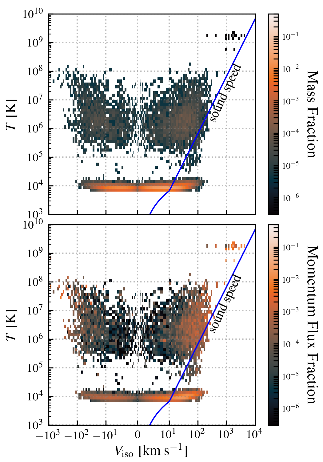
Fig. 6 shows the phase structure of the fiducial run 5e-2–j1e4–n1e5–T1e4 in the temperature – (isotropic component of cocoon velocity) plane. The top panel is mass-weighted, showing the phase distribution, while the bottom panel is momentum-flux-weighted, showing which phase contributes the most to the outflowing momentum flux. There are clearly two phases present. The first is the hot phase, which consists of the reverse-shocked hot gas filling the volume of the cocoon, and is primarily trans- to subsonic-turbulent. The second, colder, phase is roughly at the background gas temperature and density. The gas in this phase is at the “mixing layer” of the cocoon and surrounding gas, which is already cold. The second panel shows that both phases have a roughly equivalent contribution to the outflowing cocoon momentum flux, while most of the mass is in the cold phase.
Fig. 7 shows an estimate of how the cocoon gas properties depend on the background gas properties at the Bondi radius. This is represented as and in Eq. (6). We note that the dependence on the jet velocity is weak (), so we do not explicitly show it here. Given what we saw in Fig. 6, we fit for the gas properties of the whole cocoon (estimated as , shown with green lines), the cool-mixing-layer phase (; blue lines), and the hot cocoon gas (; red lines). We include only gas with . While averaging the cocoon gas properties, we volume-weighted the density and pressure while mass-weighting the temperature and entropy. We emphasize that this yields only an approximate estimate of the power law index, as each jet model goes through multiple cycles of feedback and the cocoon consists of multi-phase gas. To look at overall behaviour, we average over all times and the multi-phase cocoon gas at the Bondi radius, and fit a straight line through the results (in logarithmic quantities).
We see from the left panel that the cold-mixing-layer gas generally follows the background gas temperature and density. On the other hand, the hot cocoon gas follows a constant entropy trend, as the reverse-shock heated gas has its properties set largely by the jet model instead of the background gas properties. We find a scaling approximately with , consistent with our claim in § • ‣ 4.3 that the higher the background density, the more elongated the cocoon.
The right panel shows that the cocoon gas, in either phase, scales only weakly with the background temperature. Again, the cold-mixing-layer gas roughly matches the background gas temperature since they have both already cooled to the temperature floor (). On the other hand, the hot phase has a steeper than linear scaling with the background temperature. Overall, we find a scaling of with . This is also roughly consistent with our claim in § • ‣ 4.3 that, if is smaller than 0, the higher the background temperature, the more “isotropic” the jet cocoon (§ • ‣ 4.3).
5.3 The black hole accretion rate and jet mass flux
Having determined how the cocoon properties depend on the background gas density and temperature, we can finally see whether the implied regulation of our jet and the resulting black hole accretion rate in our simple model can qualitatively explain what we see in the simulations. Fig. 8 shows the time-averaged jet mass flux in all of the runs, with each panel showing the variation of a specific parameter. We plot only the jet mass flux for ease of comparison with our simple model, but it should be kept in mind that this is directly proportional to the black hole accretion rate (simply scaled by a constant factor , which is for most runs).
The first panel shows that the jet mass flux is independent of the feedback mass fraction. The jets in these runs have the same specific energy, so the same jet mass flux means the same momentum and energy flux, which implies a very similar cocoon propagation. With the lower feedback mass fraction, the black hole accretes more to provide an equivalent level of feedback. This holds until the required accretion rate is much larger than the Bondi accretion rate, in which case the jet model will fail to self-regulate. That scenario is not within the parameter space we simulate here.
In the second panel, we vary the kinetic fraction by varying the jet temperature and velocity while keeping the total specific energy the same. The lower kinetic fraction run has most of the energy in a thermal component, isotropizing the cocoon essentially at the launch of the jet. Moreover, since its cocoon has never been in a momentum conserving phase, it does not reach far beyond the Bondi radius. It can clearly be seen in the last rows of Fig. 4 and Fig. 5 that, although the isotropic component of the cocoon momentum flux matches the Bondi value at the Bondi radius in both the thermal and kinetic jets, the cocoon momentum flux decays more steeply beyond the Bondi radius. As a result, much less energy is “wasted” beyond the Bondi radius, so both the jet mass flux and black hole accretion rates regulate to a lower value.
In the simulations where we vary the jet velocity (center-left panel), the cocoon density depends weakly on the jet velocity, as mentioned in § 5.2. Therefore Eq. (4.2.1) () predicts a scaling of , and Eq. (4.2.2) () predicts a scaling of . These scaling relations roughly match what we see in Fig. 8. We plot the scaling relations fit to all of the runs with velocities (more elongated cocoon), and with velocities (more bubble-like). As expected, the fits for the more elongated cocoon predict a steeper jet velocity dependence than the isotropic bubble case. It is also slightly steeper than what we predict from our simple model, but we re-emphasize that we are fitting a line to a small number of points and this result should be seen as a rough estimate.
When we vary the gas temperature (center-right panel), we find a scaling relation . This is qualitatively consistent but a bit steeper than our model (Eq. 4.2.2 and Eq. 4.2.1 with ), which implies a scaling to with a power-law index of 0 to -0.18 (cocoon) or -0.5 to -0.7 (bubble).
Finally, when we vary the gas density (bottom-left panel), the cocoon gas density depends on the background gas density as with . Therefore Eq. (4.2.2) and Eq. (4.2.1) predict with . We plot the scaling relations fit to the runs with density (more elongated cocoon), and with density (more bubble-like). The first scenario has a similar scaling relation to our toy model. The latter case results in a somewhat steeper slope, which qualitatively agrees with our toy model but is steeper than predicted.
5.4 The growth of the black hole
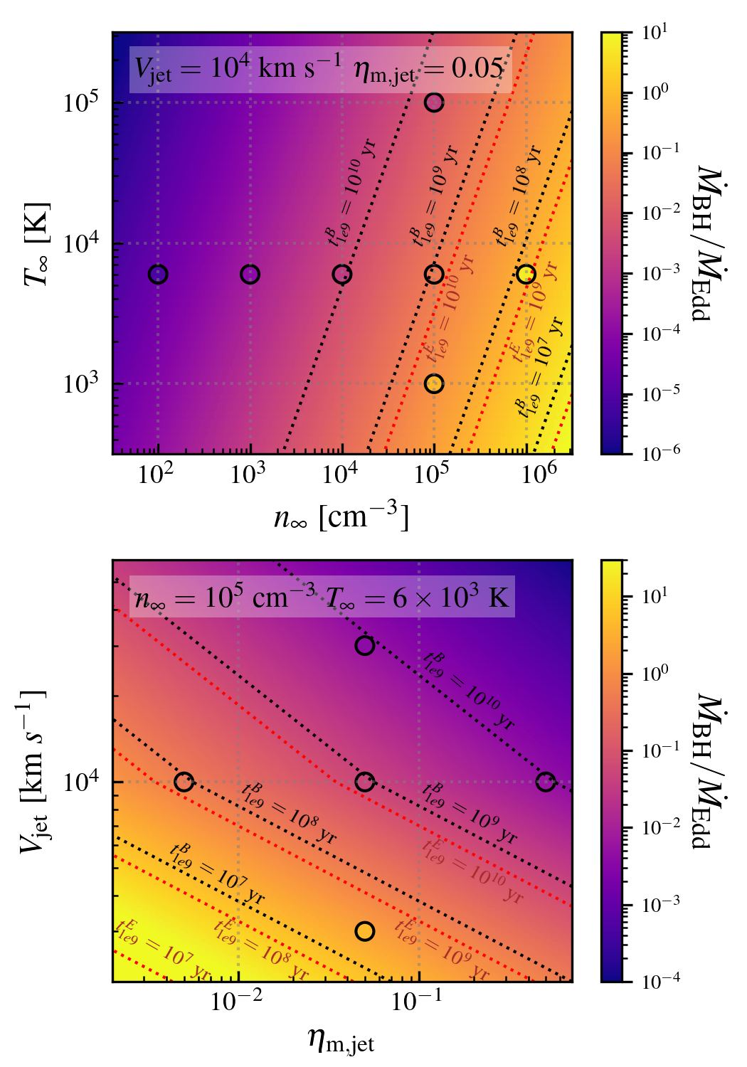
We indicate the mean time-averaged black hole accretion rate of each model in Table 1. The runs with the highest accretion rate are, unsurprisingly, the runs with the lowest feedback mass fraction (), the lowest relative specific energy (that is the lowest jet velocity, ), the highest background density (), and the lowest temperature (). They can all accrete at super-Eddington rates at their peak, reaching an accretion rate of or (0.4-6) on average, where the reference Eddington accretion rate relates to the Eddington luminosity as (although we remind readers that we are not treating radiative feedback in this work). In our surveyed parameter space, the presence of jet feedback suppresses the accretion rate below the Bondi rate by factors ranging from up to 0.7. Note that there is a strong time variability of the black hole accretion rate and the resulting jet fluxes (see Fig. 2). We only run the simulations for yr, so none of the black holes grow significantly during the short periods covered by the simulations. Nevertheless, these results indicate that, for at least some of our model parameters, the black hole could grow to very large masses in cosmologically short times if it continues to be surrounded by high density gas.
We can express the ratio using the scalings predicted by our toy model, normalized to the fiducial parameter choices, as
| (25) |
where the exponent of ranges from 2 (for ) to 3 (for ). Assuming the separation of the two cases is roughly at , we plot the estimated BH accretion rate in Fig. 9. On top of the toy-model prediction, we indicate the results from our runs with circles colored with their measured values, and they show a qualitative agreement. We also show a set of dashed lines showing the parameters for which the estimated time needed for a 100 black hole to grow to () is , , , and years. Since we only performed simulations for a single BH mass, , in this study, this requires extrapolating the time-averaged accretion rates to higher BH masses. The calculation of assumes (corresponding to a fixed fraction of the Bondi rate, with fixed background gas properties) throughout the evolution. This is motivated by the dependence of predicted in our toy model (see Eq. (4.2.1) and Eq. (4.2.2)) but will be left for future study to verify with simulations with different black hole masses. For a less optimistic estimate, the calculation of instead assumes (corresponding to a fixed fraction of the Eddington rate) throughout the evolution. Given the assumptions above and the estimated accretion rate of each case at , part of the parameter space can have a 100 black hole growing to a supermassive black hole at high redshift. We emphasize that these are crude estimations. The underlying assumptions of a fixed fraction of Bondi accretion and the constant background gas properties are subject to verification in future work.
5.5 Jet duty cycle
Besides regulating the black hole accretion rate and jet mass flux, the various jet models and background gas properties also affect the feedback cycle period. A run with a more elongated jet cocoon that propagates to a larger distance will result in longer-term variability in the accretion rate. This can be seen in the left panel of Fig. 10, where we quantify the normalized (i.e. divided by its maximum value) power spectrum of the BH accretion rate in the runs with different velocities. We clearly see that the slower the jet velocity, the more elongated the jet cocoon becomes and the more the power spectrum shifts to longer periods (lower frequencies). The reason for this behavior is simply that, when the jet reaches a larger distance, the time scale of the regulation (i.e., the free fall time) becomes longer.
Similarly, changing the gas temperature also impacts the distance that the cocoon reaches. In the right panel of Fig. 10, we see that the higher temperature run, which has the smaller Bondi radius, has a power spectrum shifted to shorter periods.
6 Discussion
6.1 Comparison with previous works
Regan et al. 2019 used the adaptive mesh refinement (AMR) hydrodynamics code ENZO to investigate feedback from bipolar jets, expected to be produced during super-Eddington accretion episodes, focusing on how the jet feedback impacts BH growth. They found that the jets periodically evacuate the central pc region, and accretion then resumes after a free-fall time. Overall, we here find a similar behaviour, although there are several differences between our setups and our results. Regan et al. 2019 utilize a cosmological simulation, and adopt an initial seed BH mass of , with an initial accretion rate of , and find that the time-averaged accretion rate always stays below the Eddington value. Also, once the gas is heated by the jet, they do not resolve the Bondi radius, and adopt a modified Bondi accretion rate. By comparison, we here use an initially uniform and static cloud, and examine a times lower BH mass, times lower accretion rate, and a times higher spatial resolution, such that the Bondi radius remains resolved at all times. We find that super-Eddington accretion is possible, which may be explained by the different parameter choices and/or differences in the details in the shapes of the jet-driven cocoons. Another difference between our studies is that we examine the cocoon evolution in greater detail and offer a physical interpretation of its shape and size, as a function of jet and background gas parameters.
Park & Ricotti 2011 studied a similar problem regarding accretion onto a low-mass black hole, but with radiative feedback instead of the mechanical jet feedback explored here. They obtain a scaling of the time-averaged black hole accretion rate with background gas properties ( for and for ), which are different from ours. The primary reason is that the radiative feedback they implemented inflates a roughly constant temperature bubble around the black hole, which is in pressure equilibrium with the surrounding cold gas. This is very different from the cocoon we see inflated by jet feedback, where the cocoon has a more complicated shape as discussed in § 4. Park & Ricotti 2011 also found a feedback cycle with a well-defined period, while we have much more complicated cycles. This can arise from the more anisotropic turbulent gas distribution due to the jetted feedback or the more complex geometry of the outflows and accretion. The fact that we are using 3D simulations, while Park & Ricotti 2011 used 1D and 2D simulations, could also contribute to the difference. Overall, the time-averaged accretion rate in Park & Ricotti 2011 was found to always remain below the Eddington rate, whereas we here find super-Eddington accretion in many cases. This suggests that jet feedback may be a lesser obstacle to BH growth than radiative feedback.
Takeo et al. 2020 also studied a similar problem with different black hole masses ( and ) and with wider AGN winds on top of radiative feedback. They focused on the ’hyper-Eddington’ regime, such that the Bondi rate exceeds the Eddington rate by several orders of magnitude. In practice, they considered either a much higher BH mass or a much higher background gas density than in our study. They showed that under these conditions, the resulting accretion rate can remain close to the Bondi accretion rate and reach the prescribed hyper-Eddington values after around a dynamical time, when the radiative feedback becomes less important. They also found that the accretion rate is insensitive to the feedback mass fraction of the mechanical feedback. These latter findings are qualitatively similar to what we see in our simulations with the AGN jet, despite different initial velocity and initial open-angle. They also see momentum conserving wind propagation (constant velocity) all the way to beyond Bondi radius, qualitatively similar to what we see in our lower velocity jets, which is also expected in our toy model. Given the difference in the feedback form, black hole mass, and run time, and background Bondi accretion rate, more quantitative comparisons would be difficult.
It is worth also comparing our results with the jets in larger-scale galaxy simulations, e.g. those presented in Su et al. 2021. A similar qualitative result was found in those galaxy scale studies, namely that heavier jets result in much narrower jet cocoons which propagate much farther. The toy model describing the jet propagation presented in § 4 also works on galaxy scales with a much more massive black hole and lower gas density. One important difference is the relative strength of radiative cooling, which operates more rapidly in the current simulations. Here, we find significant cooling at the contact discontinuity between the shocked jet material and the shocked ambient medium, whereas cooling on the cluster and galaxy scale is slower and occurs mostly in gas which is not shock-heated.
Massonneau et al. 2022 also examined the impact of jet feedback on BH growth on larger (kpc scales), in a dark matter halo and found that mildly super-Eddington accretion is possible. They found that weaker super-Eddington jets allow for more rapid BH growth through more frequent super-Eddington episodes, and also that weaker jet feedback efficiency leads to larger BH masses, which are consistent with our findings.
6.2 Connection to other scales
Part of the motivation of this work, where we perform intermediate-scale simulations, is to provide insight in connecting galaxy scale simulations and GRMHD simulations that can resolve the accretion disk. Depending on the galaxy size and the numerical method, the finest resolution of the former case is at best pc, and generally much lower (Wetzel et al. 2016; Su et al. 2018; Wheeler et al. 2019; Massonneau et al. 2022, e.g.,). The outer boundary of the latter case is at most ( is the gravitational radius; e.g. Lalakos et al. 2022), which is roughly pc, implying a order of magnitude gap for the black hole mass we model here. Our simulation, with its outer boundary at roughly pc and a maximum resolution of pc fits between these scales, although we note that we are still far from .
Unless using GRMHD simulations, which resolve the gravitational radius, AGN jets are not self-consistently launched but are implemented instead with sub-grid prescriptions. Effectively these sub-grid “jet models” attempt to inject the fluxes of a ”cocoon” inflated by a jet launched on an even smaller scale. Therefore, even identical jet energy, momentum, and mass fluxes can produce different physical behaviour when launched on different scales. This work provides a framework for coarse-graining jet models launched on a smaller scale to the resolution scale of galaxy simulations. The toy model described in § 4 and verified in our simulations describes how the cocoon energy, momentum, and mass flux should scale as a function of radius. The scalings can be incorporated into simulations on different scales for the same sub-grid jet model.
Effectively, given a certain estimated density () and temperature () around a black hole, and a jet model () on a small scale, , Eq. (22) can roughly determine whether is larger or smaller than . Depending on which side it falls, the resulting time-averaged can be estimated through Eq. (4.2.1) or Eq. (4.2.2). Note that we also need the , , and values from the fit results in Fig. 7. Assuming we want to find the effective cocoon property at a given larger radius, , the cocoon expansion either follows Eq. (4.1.1) and Eq. (4.1.1) (if ) or Eq. (4.1.2) (if ). Therefore, with the values , , , , , , and , we find the corresponding cocoon expansion velocity at a specific radius , which can be used as an “effective” coarse-grained jet model at that scale. The aforementioned implementation should, of course, be explicitly tested in galaxy-scale simulations. Indeed, besides the effective velocities, there is also the complexity of an “effective” jet model, including the temperature, time variability, gas cooling, and the exact sampling of the velocity distribution while launching the feedback. We leave a thorough investigation of these issues, and the construction of a full sub-grid jet recipe, to future work.
6.3 Limitations of this work and future prospects
We emphasize that we have deliberately considered an idealized setup, with an initially static cloud with a uniform density and temperature. In reality, the gas surrounding the black hole could be highly turbulent with a non-zero net angular momentum. We also consider only one black hole mass (see e.g., Regan et al. 2019; Takeo et al. 2020; Massonneau et al. 2022, for similar studies with larger black holes. ). Moreover, this work does not include magnetic fields, conduction, viscosity, and other plasma physics, which may be important on these scales.
For the feedback itself, we only include jet feedback in this work for simplicity, ignoring any radiative feedback (Park & Ricotti 2011; Regan et al. 2019; Takeo et al. 2020, e.g.,), which may also play an important role in the black hole’s neighborhood. Due to the limitations of non-relativistic hydrodynamics, we also limit the jet velocity to . This should be reasonable at the jet launching scale of our simulations but might not cover the whole possible parameter space in more extreme circumstances. We also did not explore models with wider opening-angle AGN winds (Takeo et al. 2020, e.g.,). Cosmic rays might be another critical aspect of AGN feedback as well (Su et al. 2020; Su et al. 2021; Wellons et al. 2022), but are not included here. We will explore these aspects in future work.
7 Conclusion
In this work, we utilized high-resolution hydrodynamic simulations of 0.4-1.6 pc boxes with uniform initial density and temperature to study jet propagation and its effect on black hole accretion onto a 100 black hole in low metallicity dense gas. We found that the isotropic component of the cocoon momentum flux regulates the black hole accretion and the mass, momentum, and energy flux from the AGN jet. We summarize our major conclusions as follows:
- •
After a jet is launched, it inflates a jet cocoon filled with a hot reverse shock-heated turbulent gas and a much cooler gas phase at the mixing layer with the surrounding gas.
- •
At launch, a jet cocoon will propagate, conserving the momentum in the jet direction while continuously broadening itself through thermal pressure in the lateral directions. Eventually, the cocoon expands laterally and the propagation in the jet direction slows down. If the jet cocoon propagates to a sufficiently large radius, it eventually evolves into a quasi-spherical bubble. After that, the cocoon propagates isotropically in an energy-driven scenario.
- •
Depending on the jet and background gas properties, the inflated cocoon either isotropizes beyond the Bondi radius (retaining an elongated shape), or inside the Bondi radius (becoming spherical bubble-like).
- •
In either case, the isotropic component of the cocoon momentum flux (roughly twice the lateral momentum flux if the cocoon is elongated) on average matches the inflow momentum flux at the Bondi radius, assuming a Bondi-accretion scenario. This, in turn, regulates the black hole accretion.
- •
We presented a toy model based on this picture which results in a scaling of the black hole accretion rate that roughly matches the rate found in the simulations.
- •
The lower the jet velocity and the higher the background gas density, the more elongated the jet cocoon.
- •
In addition to the average black hole accretion rate and jet mass flux, the different jet model and background gas properties also affect the accretion history variability. A jet model that produces an elongated cocoon propagates to a larger distance and produces longer-timescale variability, while smaller and more spherical bubble-like cocoons produce shorter-timescale variability. Higher (smaller ) also leads to more short-timescale variability.
- •
The runs with the highest accretion rates are those with the lowest feedback mass fraction (), the lowest specific energy or jet velocity (), the highest density (), or the lowest temperature (). They, on average, have super Eddington accretion, . In our surveyed parameter space, the presence of AGN jets suppresses the Bondi accretion rate by factors from to .
In summary, this work shows how different jet models (and background gas properties) result in different cocoon properties and accretion rates. Our results suggest that at least initially, stellar-mass black holes in so-called ’atomic cooling haloes’ may be able to grow at rates well above the Eddington rate. Our study also suggests a prescription to link simulations on different scales (§ 6.2). Many caveats and unanswered questions remain (see § 6.3) to be explored in future work.
Acknowledgements
Numerical calculations were run on the Flatiron Institute cluster “popeye” and “rusty” and allocations TG-PHY220027 and TG-PHY220047 granted by the Engineering Discovery Environment (XSEDE) supported by the NSF. KS acknowledges support from Simons Foundation. GLB acknowledges support from the NSF (OAC-1835509, AST-2108470), a NASA TCAN award, and the Simons Foundation. ZH acknowledges support from NSF grant AST-2006176. RSS and CCH were supported by the Simons Foundation through the Flatiron Institute. CAFG was supported by NSF through grants AST-1715216, AST-2108230, and CAREER award AST-1652522; by NASA through grants 17-ATP17-006 7 and 21-ATP21-0036; by STScI through grants HST-AR-16124.001-A and HST-GO-16730.016-A; by CXO through grant TM2-23005X; and by the Research Corporation for Science Advancement through a Cottrell Scholar Award.
Data Availability statement
The data supporting the plots within this article are available on reasonable request to the corresponding author. A public version of the GIZMO code is available at http://www.tapir.caltech.edu/phopkins/Site/GIZMO.html.
References
- Alvarez et al. (2009a) Alvarez M. A., Wise J. H., Abel T., 2009a, ApJ, 701, L133
- Alvarez et al. (2009b) Alvarez M. A., Wise J. H., Abel T., 2009b, ApJ, 701, L133
- Anglés-Alcázar et al. (2017) Anglés-Alcázar D., Davé R., Faucher-Giguère C.-A., Özel F., Hopkins P. F., 2017, MNRAS, 464, 2840
- Anglés-Alcázar et al. (2021) Anglés-Alcázar D., et al., 2021, ApJ, 917, 53
- Begelman & Cioffi (1989) Begelman M. C., Cioffi D. F., 1989, ApJ, 345, L21
- Bîrzan et al. (2004) Bîrzan L., Rafferty D. A., McNamara B. R., Wise M. W., Nulsen P. E. J., 2004, ApJ, 607, 800
- Bondi (1952) Bondi H., 1952, MNRAS, 112, 195
- Bosman (2022) Bosman S. E. I., 2022, Zenodo
- Bourne & Sijacki (2017) Bourne M. A., Sijacki D., 2017, MNRAS, 472, 4707
- Bradford et al. (2018) Bradford J. D., Geha M. C., Greene J. E., Reines A. E., Dickey C. M., 2018, ApJ, 861, 50
- Dickey et al. (2019) Dickey C. M., Geha M., Wetzel A., El-Badry K., 2019, ApJ, 884, 180
- Dubois et al. (2010) Dubois Y., Devriendt J., Slyz A., Teyssier R., 2010, MNRAS, 409, 985
- Fabian (2012) Fabian A. C., 2012, ARA&A, 50, 455
- Gaspari et al. (2012) Gaspari M., Brighenti F., Temi P., 2012, MNRAS, 424, 190
- Greene et al. (2006) Greene J. E., Ho L. C., Ulvestad J. S., 2006, ApJ, 636, 56
- Guo (2015) Guo F., 2015, ApJ, 803, 48
- Hickox & Alexander (2018) Hickox R. C., Alexander D. M., 2018, ARA&A, 56, 625
- Hopkins (2015) Hopkins P. F., 2015, MNRAS, 450, 53
- Hopkins & Quataert (2011) Hopkins P. F., Quataert E., 2011, MNRAS, 415, 1027
- Hopkins et al. (2016) Hopkins P. F., Torrey P., Faucher-Giguère C.-A., Quataert E., Murray N., 2016, MNRAS, 458, 816
- Hopkins et al. (2018) Hopkins P. F., et al., 2018, MNRAS, 480, 800
- Inayoshi et al. (2016) Inayoshi K., Haiman Z., Ostriker J. P., 2016, MNRAS, 459, 3738
- Inayoshi et al. (2020) Inayoshi K., Visbal E., Haiman Z., 2020, ARA&A, 58, 27
- Jiang et al. (2014) Jiang Y.-F., Stone J. M., Davis S. W., 2014, ApJ, 796, 106
- Krause (2003) Krause M., 2003, A&A, 398, 113
- Lalakos et al. (2022) Lalakos A., et al., 2022, arXiv e-prints, p. arXiv:2202.08281
- Li & Bryan (2014) Li Y., Bryan G. L., 2014, ApJ, 789, 54
- Li et al. (2015) Li Y., Bryan G. L., Ruszkowski M., Voit G. M., O’Shea B. W., Donahue M., 2015, ApJ, 811, 73
- Manzano-King et al. (2019) Manzano-King C. M., Canalizo G., Sales L. V., 2019, ApJ, 884, 54
- Martizzi et al. (2019) Martizzi D., Quataert E., Faucher-Giguère C.-A., Fielding D., 2019, MNRAS, 483, 2465
- Massonneau et al. (2022) Massonneau W., Volonteri M., Dubois Y., Beckmann R. S., 2022, arXiv e-prints, p. arXiv:2201.08766
- Mezcua & Lobanov (2011) Mezcua M., Lobanov A. P., 2011, Astronomische Nachrichten, 332, 379
- Mezcua et al. (2013a) Mezcua M., Farrell S. A., Gladstone J. C., Lobanov A. P., 2013a, MNRAS, 436, 1546
- Mezcua et al. (2013b) Mezcua M., Roberts T. P., Sutton A. D., Lobanov A. P., 2013b, MNRAS, 436, 3128
- Mezcua et al. (2015) Mezcua M., Roberts T. P., Lobanov A. P., Sutton A. D., 2015, MNRAS, 448, 1893
- Mezcua et al. (2018a) Mezcua M., Civano F., Marchesi S., Suh H., Fabbiano G., Volonteri M., 2018a, MNRAS, 478, 2576
- Mezcua et al. (2018b) Mezcua M., Kim M., Ho L. C., Lonsdale C. J., 2018b, MNRAS, 480, L74
- Mezcua et al. (2019) Mezcua M., Suh H., Civano F., 2019, MNRAS, 488, 685
- Milosavljević et al. (2009) Milosavljević M., Bromm V., Couch S. M., Oh S. P., 2009, ApJ, 698, 766
- Nyland et al. (2012) Nyland K., Marvil J., Wrobel J. M., Young L. M., Zauderer B. A., 2012, ApJ, 753, 103
- Nyland et al. (2017) Nyland K., et al., 2017, ApJ, 845, 50
- Park & Ricotti (2011) Park K., Ricotti M., 2011, ApJ, 739, 2
- Penny et al. (2018) Penny S. J., et al., 2018, MNRAS, 476, 979
- Prasad et al. (2015) Prasad D., Sharma P., Babul A., 2015, ApJ, 811, 108
- Regan et al. (2019) Regan J. A., Downes T. P., Volonteri M., Beckmann R., Lupi A., Trebitsch M., Dubois Y., 2019, MNRAS, 486, 3892
- Reines & Deller (2012) Reines A. E., Deller A. T., 2012, ApJ, 750, L24
- Reines et al. (2014) Reines A. E., Plotkin R. M., Russell T. D., Mezcua M., Condon J. J., Sivakoff G. R., Johnson K. E., 2014, ApJ, 787, L30
- Ruszkowski et al. (2017) Ruszkowski M., Yang H.-Y. K., Zweibel E., 2017, ApJ, 834, 208
- Sadowski et al. (2014) Sadowski A., Narayan R., McKinney J. C., Tchekhovskoy A., 2014, MNRAS, 439, 503
- Sbarrato et al. (2021) Sbarrato T., Ghisellini G., Giovannini G., Giroletti M., 2021, A&A, 655, A95
- Sbarrato et al. (2022) Sbarrato T., Ghisellini G., Tagliaferri G., Tavecchio F., Ghirlanda G., Costamante L., 2022, arXiv e-prints, p. arXiv:2203.09527
- Shakura & Sunyaev (1973) Shakura N. I., Sunyaev R. A., 1973, A&A, 500, 33
- Springel et al. (2005) Springel V., Di Matteo T., Hernquist L., 2005, MNRAS, 361, 776
- Su et al. (2018) Su K.-Y., et al., 2018, MNRAS, 480, 1666
- Su et al. (2020) Su K.-Y., et al., 2020, MNRAS, 491, 1190
- Su et al. (2021) Su K.-Y., et al., 2021, MNRAS, 507, 175
- Takeo et al. (2020) Takeo E., Inayoshi K., Mineshige S., 2020, MNRAS, 497, 302
- Torrey et al. (2020) Torrey P., et al., 2020, MNRAS, 497, 5292
- Volonteri et al. (2021) Volonteri M., Habouzit M., Colpi M., 2021, Nature Reviews Physics, 3, 732
- Webb et al. (2012) Webb N., et al., 2012, Science, 337, 554
- Weinberger et al. (2017) Weinberger R., Ehlert K., Pfrommer C., Pakmor R., Springel V., 2017, MNRAS, 470, 4530
- Wellons et al. (2022) Wellons S., et al., 2022, arXiv e-prints, p. arXiv:2203.06201
- Wetzel et al. (2016) Wetzel A. R., Hopkins P. F., Kim J.-h., Faucher-Giguère C.-A., Kereš D., Quataert E., 2016, ApJ, 827, L23
- Wheeler et al. (2019) Wheeler C., et al., 2019, MNRAS, 490, 4447
- Wrobel & Ho (2006) Wrobel J. M., Ho L. C., 2006, ApJ, 646, L95
- Wrobel et al. (2008) Wrobel J. M., Greene J. E., Ho L. C., Ulvestad J. S., 2008, ApJ, 686, 838
- Yang & Reynolds (2016) Yang H.-Y. K., Reynolds C. S., 2016, ApJ, 818, 181
- Yang et al. (2012) Yang H. Y. K., Sutter P. M., Ricker P. M., 2012, MNRAS, 427, 1614
Appendix A Resolution Study and the variations of accretion models
| Accretion model | ||||||
| Model | Box size | |||||
| kyr | pc | pc | kyr | |||
| pc | ||||||
| high res | 40-80 | 0.4 | 1.7e-7 | 3e-8 | 0.003 | No |
| low res | 100 | 0.4 | 1.4e-6 | 1e-7 | 0.003 | No |
| pc | ||||||
| high res | 100 | 0.4 | 1.7e-7 | 3e-8 | 0.03 -0.15 | No |
| low res | 100 | 0.4 | 1.4e-6 | 1e-7 | 0.03 -0.15 | No |
| pc + disk | ||||||
| 100 yr | 100 | 0.4 | 1.4e-6 | 1e-7 | 0.03-0.15 | 0.1 |
| 1000 yr | 100 | 0.4 | 1.4e-6 | 1e-7 | 0.03-0.15 | 1 |
| 10000 yr | 100 | 0.4 | 1.4e-6 | 1e-7 | 0.03-0.15 | 10 |
This is a partial list of simulations that explore resolution and numerical parameter choice. All simulations are run with (, , , and ). Columns list: (1) Model name: The naming of each model starts with the feedback mass fraction, followed by the jet velocity in km s-1 for kinetic jet or jet temperature in K for thermally dominant jets. The final two numbers label the background gas density in cm-3 and temperature in K. (2) : Simulation duration. (3) Box size of the simulation. (4) : The highest mass resolution. (5) : The mass resolution of the spawned jet particles. (6) : Sink radius in pc. (7) : Viscous time scale for alpha disk in kyr.
Fig. 11 summarizes the effects of different choices of sink radius and alpha disk model on black hole accretion rates under different resolutions. All the runs match our fiducial parameter choice (, , , and ). The first 3 rows shows the averaged value to the point at the specific time of the simulation. Most simulations are run with different variations of the random component to quantify the stochastic effect (different lines in the same color). A list of different simulations is summarized in Table 2.
With the smallest sink radius ( pc), the stochastic effects result in a factor of 2-3 span in the final results indicating a substantial stochastic effect. The higher resolution runs also result in a factor of 2-3 higher . The small sink radius also leads to the occasional formation of a disky structure right around the black hole at high resolution, which partially contributes to the more significant resolution dependence. Given that we do not have the proper resolution and physics to model the accretion disk explicitly, we shift to a larger sink radius and put in a subgrid -disk model as described in the main paper.
The runs with a larger sink radius ( pc) 44 4 The sink radius is set to be a radius from the black hole enclosing 96 “weighted” neighborhood gas particles but capped to be within ( pc). have a slightly smaller dependence on resolution and smaller stochastic effects (everything within ), partially due to the suppression of an artificial disky structure at very small radius. This level of difference (even the small sink radius runs) is smaller than the difference caused by most of the physics variations Fig. 2 and Fig. 8. In our production run, we adopt the larger sink radius ( pc). Given the smaller resolution dependence with this sink radius, we try to match the lower resolution for most of our physical variations for lower computational cost.
The models with alpha disk and different viscous time scales also result in differences within a factor of two, within the stochastic range, and roughly have the same accretion rates as the runs without an alpha disk. The final row of Fig. 11 shows the real-time of the runs with different viscous time scales. Shorter time scale results in a shorter-term variation. We adopt yr in our productive runs according to an estimate of the viscous time scale at the sink radius we choose (see § 2).