Quantum-inspired variational algorithms for partial differential equations: Application to financial derivative pricing

McLachlan’s variational principle [18] is an example of a time-dependent variational principle (TDVP) that approximates the solution of the TDSE by evolution within a space of parametrized trial functions. TDVPs for the TDSE have been devised for tensor network states [12], neural-network quantum states (NQS) [5] and parametrized quantum circuits [25, 2]. Ref. [24] studied TDVPs through the lens of information geometry providing a unified perspective applicable to variational quantum algorithms (VQAs) and variational quantum Monte Carlo with normalized neural-network quantum states. In the following section, we further generalize TDVPs to include general time-dependent PDEs and establish additional connections with the VQA and numerical analysis literature. Given a time-dependent PDE for the state variable $u(t,x)\in\mathbb{C}$ with $(t,x)\in[0,T]\times\Omega$, together with a choice of parametrized functions of the spatial variable $\{u_{\theta}:\Omega\longrightarrow\mathbb{C}\,|\,\theta\in\mathbb{R}^{p}\}$, the output of a TDVP is parametrized curve $\gamma:[0,T]\longrightarrow\mathbb{R}^{p}$ in the space of variational parameters such that $u_{\gamma(t)}$ optimally describes $u(t,\cdot)$ in some distance metric $\operatorname{dist}(\cdot,\cdot)$ for all $t\in[0,T]$. Consider the initial value problem for a general time-dependent PDE of the form,

with prescribed boundary conditions on $\partial\Omega$. In order to simplify exposition, in this section we avoid complications of boundary conditions by assuming either $\Omega=\mathbb{R}^{d}$ with suitable decay at infinity or $\Omega=\mathbb{T}^{d}$. In practice we replace the spatial domain by a mesh $\widehat{\Omega}\subset\Omega$, thereby approximating square-integrable functions by square summable vectors. The imposition of boundary conditions on the spatial mesh is then achieved via the use of source functions. Let $\Phi^{t}_{s}$ denote the time evolution map for state variable such that $\Phi^{t}_{u}\circ\Phi^{u}_{s}=\Phi^{t}_{s}$ and in particular $u(t,\cdot)=\Phi^{t}_{0}(u_{0})$. Given an initial parameter vector $\theta_{0}\in\mathbb{R}^{p}$ and a step size $\delta t>0$, define a sequence of parameter vectors $(\theta_{k})_{k\in\mathbb{N}}$ by the following iteration

In quantum physics applications, a suitable distance metric is the Fubini-Study metric, as previously argued both in VMC [5, 24] and in VQA [25, 2] literature. In this work we choose $\operatorname{dist}(\cdot,\cdot)$ to be the Euclidean norm. Rather than solving the discrete-time dynamical system (3) directly, we consider the limit of infinitesimal step size $\delta t\longrightarrow 0$ in which it reduces to the following system of ordinary differential equations (ODEs)¹¹ 1 See appendix A for a derivation. Similiar ODEs have been introduced in the neural Galerkin method [4]. with initial condition $\gamma(0)=\theta_{0}$:

where

and where $\langle\cdot|\cdot\rangle$, $\|\cdot\|_{2}$ denote the standard inner product and the induced norm for $L^{2}(\Omega,\mathbb{C})$, respectively. Although the matrix $M_{ij}$ is necessarily positive semi-definite, it may be degenerate, reflecting the possibility of multiple minima in the optimization problem (3). Thus, regularization techniques are generally required in order to obtain a well-posed system of ODEs.

Before discussing our autoregressive neural-network quantum state implementation, it is useful to orient within scientific computing literature by showing that the formalism shares close parallels with the classic finite element method applied to the linear inhomogeneous case $\mathcal{F}(t,x,u)=\mathcal{L}u(t,x)+f(t,x)$. Given a set of real basis functions $\{\varphi_{i}\}_{i=1}^{m}$, define the variational family consisting of a weighted superposition,

where $\theta\in\mathbb{R}^{m}$ is assumed here. Substituting the above into (4) one finds the following ODE determining the dynamics of the weights,

which can be recognized as the standard discrete linear systems arising in finite element methods, with $M$ and $K$ the mass- and stiffness-matrix, respectively. Recall that since finite element techniques use non-overlapping elements to discretize the spatial domain and employ basis functions with localized support, the problem size scales as $m\sim p^{d}$ in $d$ spatial dimensions, where $p$ is the average number of elements per dimension. Thus, the curse-of-dimensionality arises from need to perform increasingly high-dimensional, albeit sparse, linear algebra in order to solve the linear system (7). The approach advocated in the following section, in contrast, overcomes the curse-of-dimensionality by representing the solution vector in terms of an autoregressive neural-network quantum state.

In order to overcome the curse of dimensionality with respect to the spatial dimension $d$, which is inherent in the utilization of a $d$-dimensional mesh $\widehat{\Omega}\subset\Omega\subseteq\mathbb{R}^{d}$, we utilize stochastic estimation combined with autoregressive assumptions. In particular, we take inspiration from both the variational quantum algorithm introduced in [1] as well variational quantum Monte Carlo using autoregressive NQS [22, 14], by parametrizing the solution of the PDE as $u_{\theta}=\alpha\,\psi_{\beta}$ where $\psi_{\beta}$ is a unit-normalized NQS with variational parameters $\beta$ and $\alpha>0$ is a scale factor, whose time-dependence must be determined from the evolution equations along with $\beta$. The variational parameters thus consist of the augmented parameter vector $\theta:=(\log\alpha,\beta)\in\mathbb{R}^{p+1}$ where $\beta\in\mathbb{R}^{p}$ is an unconstrained vector representing the weights and biases of the neural network. Plugging the rescaled ansatz into the evolution equations (4), one obtains an augmented system of first-order, non-linear ordinary differential equations determining the time-dependence of the augmented vector $\theta$. The overlaps defining $M$ and $V$ are estimated using the VMC importance sampling technique, where the probability density is chosen to be the modulus-squared wavefunction $|\psi_{\beta}(x)|^{2}$.

Rather than working in the continuum, we assume spatial discretization of the function $u(t,\cdot)$ on a regular grid $\widehat{\Omega}$ embedded in the $d$-dimensional domain $\Omega=[a_{1},b_{1}]\text{\texttimes}...\text{\texttimes}[a_{d},b_{d}]$ with a total of $2^{n}$ grid points. Without loss of generality, we assume $\Omega$ is a regular hypercube satisfying $|b_{1}-a_{1}|=...=|b_{d}-a_{d}|$, and that the mesh size along each axis is $2^{n/d}$. In order to represent the state of the discretized field in terms of the state of an $n$-qubit system, we assign each computational basis state $|k_{1},\ldots,k_{n}\rangle\in\mathbb{C}^{2^{n}}$ with $(k_{1},\ldots,k_{n})\in\{0,1\}^{n}$ to a linear index defined by $k=\sum_{i=1}^{n}k_{i}2^{i}$ and then unravel the linear index to indices along each of $d$ axes yielding a $d$-tuple $(\bar{k}_{1},\ldots,\bar{k}_{d})\in\{0,\ldots,n/d-1\}^{d}$ defined by

The mesh point $\bm{x}^{k}\in\widehat{\Omega}$ corresponding to the linear index $k\in\{0,1,...,2^{n}-1\}$ is thus

where $\Delta x=|b_{1}-a_{1}|/2^{\frac{n}{d}}$. Henceforth, we do not distinguish the index $k$, the binary string $(k_{1},\ldots,k_{n})$ and the corresponding coordinate $\bm{x}^{k}\in\widehat{\Omega}$. The digitized representation of the state of the PDE at time $t$ is thus the following unnormalized $n$-qubit state

and likewise the parametrized approximation $|u_{\theta}\rangle$ of $|u(t)\rangle$ is given by,

where $u_{\theta}(\cdot)$ is a function defined on $\widehat{\Omega}\subset\Omega$.

In order to obtain an expressive family of trial functions $u_{\theta}:\widehat{\Omega}\longrightarrow\mathbb{C}$ which furthermore admits an efficient stochastic estimation procedure, we express $u_{\theta}$ as multiple of a unit-normalized neural-network quantum state $\psi_{\beta}:\widehat{\Omega}\longrightarrow\mathbb{C}$ with variational parameters $\beta\in\mathbb{R}^{p}$,

A simple method to ensure unit-normalization and efficient sampling is to follow the work of MADE [9] which exploited a masked version of a fully connected layer, where some connections in the computational path are removed in order to satisfy the autoregressive properties, In particular, if we assume a choice of variables such that the state variable is strictly positive²² 2 This can be considered as a special case of the complex-valued case [22, 14]. $u_{\theta}(x)>0$, then a suitable choice of unit-normalized function is

where $p_{\beta,i}(\cdot|k_{i-1},\ldots,k_{1})$ is the parametrized conditional probability distribution for the $i$th bit.

Before we perform the time evolution, initial variational parameters $\theta_{0}$ must be selected in order to match the variational function $u_{\theta_{0}}(x)$ with the choice of initial condition $u_{0}(x)$ for $x\in\widehat{\Omega}$ in the spatial domain. This can be achieved via optimization of the following objective function using stochastic gradient descent,

In this section we discuss the details of the stochastic estimation of $M$ and $V$ necessary to evolve the augmented parameter vector $\theta=(\log\alpha,\beta)\in\mathbb{R}^{p+1}$. For simplicity we only consider the affine case

Consider the decomposition,

It is convenient to introduce the following helper functions. In particular, define the Born probability distribution $\rho_{\beta}(x)\in[0,\infty)$, the wavefunction score $\sigma_{\beta}(x)\in\mathbb{C}^{n}$ and the local energy $l_{\theta}(t,x)\in\mathbb{C}$ as follows,

By straightforward calculus, we obtain

and

The expectation values over $x$ are approximated using Monte Carlo sampling. In practice, the batch of randomly generated samples is represented in the form of a buffer $\mathcal{B}=\{x_{i}\}_{i=1}^{B}$ that stores the unique samples in the batch and a counter $\mathcal{C}=\{c_{i}\}_{i=1}^{B}$ that records the number of occurrences of each of the corresponding samples. Expectation values are then approximated by sums of the following form,

For initialization we chose a discrete isotropic Gaussian, expressed in terms of the modified Bessel function $I_{x}(t)$ of integer order $x$,

where $t>0$ is a parameter controlling the width of the Gaussian, and $x$ ranges from 0 to $2^{n-1}$. Pre-training was performed using Adam optimizer [16] for 50k iterations with batch size $128$, $\beta_{1}=0.9$, $\beta_{2}=0.999$, and $\epsilon=10^{-8}$. The learning rate was warm-started for the first $1/10$ total training iterations, then decayed by a factor of 10 at $3/7,5/7$ of the total training iterations.

After completion of pre-training, the state was evolved for a total evolution time $T=1$ using a step size of $\delta t=5\text{\texttimes}10^{-5}$ and a batch size of $B=1024$ for Monte Carlo estimation on each iteration. The time development of the state was compared to the result of Euler time-stepping the initial condition (27) using the same step-size. Due to the exponential scaling of the matrix $\widehat{\mathcal{L}}$, we only establish this baseline for the number of qubits $n\leq 16$. All reported numerical results are averaged across exactly 5 seeds, each trained for 20k steps.

Table 1 reports the relative error between our method and forward Euler method over 20k iterations, for diffusion problem with Dirichlet boundary conditions. The relative error of the obtained solution is computed by comparing the norm of the space-time history of the variational state with the result of Euler development,

In general, the overall solution obtained using our method matches well with that obtained using forward Euler method. Their discrepancy increases as the dimensionality of the problem increases; nonetheless, within a tolerable threshold (e.g., less than $10\%$). One remedy is to simply increase the batch size, for example, we show in Section 4.4 that the relative error improves from $15\%$ to around $3\%$ with a batch size that is ten times larger.

Since we discretize the domain $\Omega$ using a grid of size $|\widehat{\Omega}|=2^{n}$, the time complexity of forward Euler method, expressed in terms of $n$ is $O(T\text{\texttimes}2^{2n})$, where $T$ is the number of iterations. The proposed VMC algorithm, in contrast, scales as $O(TB\,\text{poly}(n))$, where $B$ is the batch size. In more detail, the forward pass scales as $O(TBn^{2})$, and the sampling is $O(TBn^{3})$, due to the sequential nature of the auto-regressive sampling process. This polynomial scaling comes at a price of the approximate nature of the time evolution step, and the implicit access to entries of the state vector compared to the forward Euler method which offers $O(1)$ lookup to entries of the state.

In Table 2, we report the average running time of both forward Euler method and our method for 2k iterations (one-tenth of the total running time). The batch size $B$ of our method is fixed to be 500. Note that we cannot apply Euler for higher dimensions due to the memory constraint. Although forward Euler method is effective for small-scale problems, its complexity suffers from the exponential growth with respect to dimension $d$. The computational cost of our method originates from four sources: sampling, forward pass, per-sample gradient computation (backward pass), and extraction of matrix element information. All these sources contribute to the overhead time that causes our method to run slower in comparison with respect to forward Euler method for problems in lower dimensions. However, as the dimensionality increases, the run time of our method grows only at a polynomial rate. It can be seen from Table 2 that our method is already faster than forward Euler for problem sizes characterized by $n=16$ qubits.

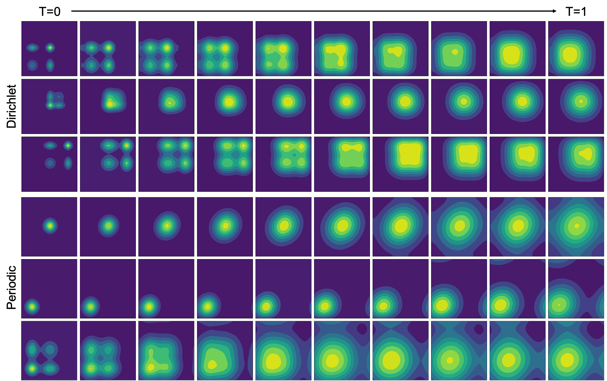
We provide snapshots of our method for 2D diffusion problems with periodic boundary conditions over 20k iterations. We run our algorithm with five distinct initializations and record the snapshot every 2k iterations. In particular we do not employ any regularization techniques to enforce that the solution satisfies the boundary condition. It can be observed in Figure 1 that our method successfully obeys the periodic boundary conditions.

Recall that $M$ and $V$ are approximated with Monte Carlo sampling using batches of unique samples. Intuitively, a larger batch size yields a better approximation to the exact expectation value, thereby providing more accurate model updates. In this section, we study the effect of batch size on the performance of our method. In the LHS of Figure 2, the running time of our algorithm increases for both larger problem sizes and batch sizes. Note that the actual running time does not grow linearly with respect to the batch size in the plot due to the cache and parallelization. In the RHS of Figure 2, we report the average relative error between the forward Euler method and the VMC method with various batch sizes. Given a fixed problem size (e.g., 4 dimensions with 4 qubits per dimension), we observe a performance improvement by increasing the batch size, which verifies our hypothesis that increasing the batch size does effectively improve the performance. Given a fixed batch size, our method performs worse as the dimensionality of the problem increases. This result implies that we need a larger batch size to guarantee good performance for problems in higher dimensions.

The Feynman-Kac stochastic representation formula links between a parabolic PDE and stochastic differential equations. Namely, consider a PDE of the form:

where $\mu:[0,T]\times\mathbb{R}^{d}\to\mathbb{R}^{d}$, $\sigma:[0,T]\times\mathbb{R}^{d}\to\mathbb{R}^{d\times d}$, $r,f:[0,T]\times\mathbb{R}^{d}\to\mathbb{R}$, and $\Phi:\mathbb{R}^{d}\to\mathbb{R}$ are given measurable functions and $H$ stands for the Hessian matrix of $u$:

Then, under a second order integrability condition, the solution to this equation takes the form:

where $(X_{t})_{t\in[0,T]}$ is the solution to the following stochastic differential equation with $(W_{t})_{t\in[0,T]}$ being a $d$-dimensional standard Wiener process:

One of the many applications of this representation is in derivative pricing. Consider multi-asset with price dynamics $(S_{t})_{t\in[0,T]}$ given by the multi-dimension geometric form:

where $\text{Diag}[x]$ is a diagonal matrix with the vector $x$ on the diagonal, $W$ is $d$-dimensional standard Wiener process, $\mu:[0,T]\times[0,\infty)\to\mathbb{R}^{d}$ and $\sigma:[0,T]\times[0,\infty)\to\mathbb{R}^{d\times d}$ are measurable and satisfy basic conditions that lead to a unique strong solution to the stochastic differential equation above. Consider also the interest rate $r:[0,T]\times[0,\infty)\to\mathbb{R}$. A risk-neutral measure is a probability measure $\mathbb{Q}$, such that the discounted price of the asset $(e^{-\int_{0}^{t}r(s,X_{s})ds}X_{t})_{t\in[0,T]}$ is a martingale under $\mathbb{Q}$. The dynamics of the multi-asset under $\mathbb{Q}$ are given by:

where $W^{\mathbb{Q}}_{\cdot}:=W_{\cdot}-\int_{0}^{\cdot}(\mu(t,S_{t})-r(t,S_{t}))dt$ is a standard Wiener process under $\mathbb{Q}$. Then, the price of a simple contingent claim with terminal payment $\Phi(S_{T})$ at any given time $t\in[0,T]$, when the multi-asset prices are $S_{t}=s$ is given by $u(t,s)$, which satisfies the PDE:

and can be expressed as the conditional $\mathbb{Q}$-expectation as follows:

The most celebrated example is the Black-Scholes model, where the dynamics of the underlying asset follows a geometric Brownian motion and the interest rate is fixed. In dimension 1, the associated PDE admits an explicit solution, which is known as the Black-Scholes formula. Aside from the fact that the solution of the PDE is the contingent claim price, its partial derivative $\partial u/\partial x$ is used in order to construct a delta-hedging portfolio. Furthermore, its partial derivatives, known as the Greeks are used to construct a robust portfolio against small changes, when moving from the continuous- to the discrete-time world.

We now demonstrate how our algorithm applied to the multidimensional heat equation can be used to price options. For this we consider the Black-Scholes model that consists of a risk-free asset with a constant risk-free return $r>0$ and $d$ risky assets whose dynamics are given by

The parameters $\mu_{i}$ and $\sigma_{i}$, $i=1,\dots,d$ are constants, and $\{W^{i}\}_{i=1}^{d}$ are Wiener processes with quadratic covariation $[W^{i}_{t},W^{j}_{t}]=\rho_{ij}t$.

Consider further a European option, whose payment at (the predetermined) expiry time $T>0$ is $\Psi(S_{T}^{1},\dots,S^{d}_{T})$, for some measurable function $\Psi$. Let $V$ be the conditional price of this option, i.e., $V(t,x_{1},\dots,x_{d})$ is the price for the option at time $t$, given that $S_{t}^{i}=x_{i}$ for $i=1,\dots,d$. It is well-known that $V$ satisfies the following Black-Scholes PDE:

Following Guillaume [10], we may reduce this $n$-dimensional equation to the $n$-dimensional standard heat equation. To this end, set

where $a_{i}$ and $b$ satisfy the following system of equations:

Then, $u$ satisfies the following heat equation

with $u(0)=\Psi(e^{\sigma_{1}y_{1}},\dots,e^{\sigma_{d}y_{d}})e^{-\sum a_{i}\sigma_{i}y_{i}}$.

In this section, we apply our algorithm to option pricing in Black-Scholes model across different settings using the numerical solution to the heat equation and the translation from the heat equation to the Black-Scholes equation from the previous subsection. We test the performance of our algorithm as well as show a calculation of the option price for higher dimensions.

In Figure 3 and Table 4 we provide examples to test the performance of our algorithm. In both we include 1D examples for the price of a European call option, whose value at the expiry time $T$ is $V(T,s)=\Psi(s)=\max\{s-K,0\}$, where $K$ is a predetermined constant, called the strike price. We vary the volatility $\sigma$, strike price $K$, interest rate $r$, expiry time $T$, and initial price of the stock $S$. In Figure 3, we compare against the forward Euler method and the ground truth Black-Scholes formula, which admits an analytical solution in 1D. Specifically, it is given by

where $N$ is the cumulative distribution function of the standard normal distribution and

Our method is robust under all settings and achieves satisfactory performance. In Table 4 we compare our accuracy against the forward Euler method, where we use the same analytical solution. Although the performance of our algorithm is inferior to that of Euler, it still achieves good accuracy and the margin can be treated as a price to pay for reducing the exponential scaling down to a polynomial one. Our approach is valuable for high dimensions, where other methods, such as the forward Euler method, suffer from the curse of dimensionality. Table 4 also includes 2D examples with four different options: Basket European call and put, rainbow max European call, and spread European put, whose payoffs are listed in Table 3. Note that as we don’t have an analytical solution for this case, the relative errors with respect to Euler solutions are reported instead. In Figure 4, we provide a graph for the price of a basket European call option with up to five underlying stocks as a function of the strike price $K$. As expected the prices are convex with $K$.

Note that the Black-Scholes PDE lives on the positive orthant of $\mathbb{R}^{d}$ while its translation to the heat equation lives on $\mathbb{R}^{d}$. Thereby, all numerical algorithms, including ours, require artificial truncation of the domain. We choose the hypercube domain to be $[s_{l},s_{u}]^{d}=[Ke^{-3\sigma_{i}\sqrt{T}},Ke^{3\sigma_{i}\sqrt{T}}]^{d}$. This choice implies that $s_{l}$ is small (close to $0+)$ and $s_{u}$ is large (close $+\infty$). On the faces of the hypercube, we use the time-discounted payoff functions, as they are reasonably accurate approximations of boundary values of the options considered. Given the number of qubits $n$ and the hypercube input domain for the heat equation $[L_{l},L_{u}]^{d}$, which is approximately $[-5,5]^{d}$, the mesh size of each axis is $(L_{u}-L_{l})/(2^{n/d}+1)$.

References

- [1] Hedayat Alghassi, Amol Deshmukh, Noelle Ibrahim, Nicolas Robles, Stefan Woerner, and Christa Zoufal. A variational quantum algorithm for the Feynman-Kac formula. arXiv preprint arXiv:2108.10846, 2021.
- [2] Stefano Barison, Filippo Vicentini, and Giuseppe Carleo. An efficient quantum algorithm for the time evolution of parameterized circuits. Quantum, 5:512, July 2021.
- [3] Christian Beck, Weinan E, and Arnulf Jentzen. Machine learning approximation algorithms for high-dimensional fully nonlinear partial differential equations and second-order backward stochastic differential equations. J. Nonlinear Sci., 29(4):1563–1619, 2019.
- [4] Joan Bruna, Benjamin Peherstorfer, and Eric Vanden-Eijnden. Neural Galerkin scheme with active learning for high-dimensional evolution equations. arXiv preprint arXiv:2203.01360, 2022.
- [5] Giuseppe Carleo and Matthias Troyer. Solving the quantum many-body problem with artificial neural networks. Science, 355(6325):602–606, 2017.
- [6] Marco Cerezo, Andrew Arrasmith, Ryan Babbush, Simon C Benjamin, Suguru Endo, Keisuke Fujii, Jarrod R McClean, Kosuke Mitarai, Xiao Yuan, Lukasz Cincio, et al. Variational quantum algorithms. Nature Reviews Physics, 3(9):625–644, 2021.
- [7] Weinan E, Jiequn Han, and Arnulf Jentzen. Deep learning-based numerical methods for high-dimensional parabolic partial differential equations and backward stochastic differential equations. Commun. Math. Stat., 5(4):349–380, 2017.
- [8] Filipe Fontanela, Antoine Jacquier, and Mugad Oumgari. A quantum algorithm for linear PDEs arising in finance. SIAM Journal on Financial Mathematics, 12(4):SC98–SC114, 2021.
- [9] Mathieu Germain, Karol Gregor, Iain Murray, and Hugo Larochelle. MADE: Masked autoencoder for distribution estimation. In International Conference on Machine Learning, pages 881–889. PMLR, 2015.
- [10] Tristan Guillaume. On the multidimensional Black-Scholes partial differential equation. Ann. Oper. Res., 281(1-2):229–251, 2019.
- [11] Irene López Gutiérrez and Christian B Mendl. Real time evolution with neural-network quantum states. Quantum, 6:627, 2022.
- [12] Jutho Haegeman, J Ignacio Cirac, Tobias J Osborne, Iztok Pižorn, Henri Verschelde, and Frank Verstraete. Time-dependent variational principle for quantum lattices. Physical review letters, 107(7):070601, 2011.
- [13] Jiequn Han, Arnulf Jentzen, and Weinan E. Solving high-dimensional partial differential equations using deep learning. Proc. Natl. Acad. Sci. USA, 115(34):8505–8510, 2018.
- [14] Mohamed Hibat-Allah, Martin Ganahl, Lauren E Hayward, Roger G Melko, and Juan Carrasquilla. Recurrent neural network wave functions. Physical Review Research, 2(2):023358, 2020.
- [15] Côme Huré, Huyên Pham, and Xavier Warin. Deep backward schemes for high-dimensional nonlinear PDEs. Math. Comp., 89(324):1547–1579, 2020.
- [16] Diederik P. Kingma and Jimmy Ba. Adam: A method for stochastic optimization. In Proc. International Conference on Learning Representations, 2015.
- [17] Zongyi Li, Nikola Kovachki, Kamyar Azizzadenesheli, Burigede Liu, Kaushik Bhattacharya, Andrew Stuart, and Anima Anandkumar. Fourier neural operator for parametric partial differential equations. arXiv preprint arXiv:2010.08895, 2020.
- [18] AD McLachlan. A variational solution of the time-dependent Schrodinger equation. Molecular Physics, 8(1):39–44, 1964.
- [19] John Preskill. Quantum computing in the nisq era and beyond. Quantum, 2:79, 2018.
- [20] Maziar Raissi, Paris Perdikaris, and George E Karniadakis. Physics-informed neural networks: A deep learning framework for solving forward and inverse problems involving nonlinear partial differential equations. Journal of Computational physics, 378:686–707, 2019.
- [21] Moritz Reh and Martin Gärttner. Variational monte carlo approach to partial differential equations with neural networks. arXiv preprint arXiv:2206.01927, 2022.
- [22] Or Sharir, Yoav Levine, Noam Wies, Giuseppe Carleo, and Amnon Shashua. Deep autoregressive models for the efficient variational simulation of many-body quantum systems. Physical review letters, 124(2):020503, 2020.
- [23] Justin Sirignano and Konstantinos Spiliopoulos. Dgm: A deep learning algorithm for solving partial differential equations. Journal of computational physics, 375:1339–1364, 2018.
- [24] James Stokes, Brian Chen, and Shravan Veerapaneni. Numerical and geometrical aspects of flow-based variational quantum monte carlo. arXiv preprint arXiv:2203.14824, 2022.
- [25] James Stokes, Josh Izaac, Nathan Killoran, and Giuseppe Carleo. Quantum natural gradient. Quantum, 4:269, 2020.
- [26] Jiangran Wang, Zhuo Chen, Di Luo, Zhizhen Zhao, Vera Mikyoung Hur, and Bryan K Clark. Spacetime neural network for high dimensional quantum dynamics. arXiv preprint arXiv:2108.02200, 2021.