Omni3D: A Large Benchmark and Model for 3D Object Detection in the Wild
Abstract
Recognizing scenes and objects in 3D from a single image is a longstanding goal of computer vision with applications in robotics and AR/VR.
For 2D recognition, large datasets and scalable solutions have led to unprecedented advances.
In 3D, existing benchmarks are small in size and approaches specialize in few object categories and specific domains, e.g. urban driving scenes.
Motivated by the success of 2D recognition, we revisit the task of 3D object detection by introducing a large benchmark, called Omni3D.
Omni3D re-purposes and combines existing datasets resulting in 234k images annotated with more than 3 million instances and 98 categories.
3D detection at such scale is challenging due to variations in camera intrinsics and the rich diversity of scene and object types.
We propose a model, called Cube R-CNN, designed to generalize across camera and scene types with a unified approach.
We show that Cube R-CNN outperforms prior works on the larger Omni3D and existing benchmarks.
Finally, we prove that Omni3D is a powerful dataset for 3D object recognition and show that it improves single-dataset performance and can accelerate learning on new smaller datasets via pre-training.11
1
We release the Omni3D benchmark and Cube R-CNN models at
https://github.com/facebookresearch/omni3d.
1 Introduction
Understanding objects and their properties from single images is a longstanding problem in computer vision with applications in robotics and AR/VR. In the last decade, 2D object recognition ren2015faster; he2017maskrcnn; tian2019fcos; law2018cornernet; redmon2016you has made tremendous advances toward predicting objects on the image plane with the help of large datasets lin2014microsoft; gupta2019lvis. However, the world and its objects are three dimensional laid out in 3D space. Perceiving objects in 3D from 2D visual inputs poses new challenges framed by the task of 3D object detection. Here, the goal is to estimate a 3D location and 3D extent of each object in an image in the form of a tight oriented 3D bounding box.
Today 3D object detection is studied under two different lenses: for urban domains in the context of autonomous vehicles chen2016monocular; mousavian20173d; brazil2019m3d; liu2020smoke; lu2021geometry or indoor scenes factored3dTulsiani17; huang2018cooperative; kulkarni2019relnet; Nie_2020_CVPR. Despite the problem formulation being shared, methods share little insights between domains. Often approaches are tailored to work only for the domain in question. For instance, urban methods make assumptions about objects resting on a ground plane and model only yaw angles for 3D rotation. Indoor techniques may use a confined depth range (e.g. up to 6m in Nie_2020_CVPR). These assumptions are generally not true in the real world. Moreover, the most popular benchmarks for image-based 3D object detection are small. Indoor SUN RGB-D song2015sun has 10k images, urban KITTI Geiger2012CVPR has 7k images; 2D benchmarks like COCO lin2014microsoft are 20 larger.
We address the absence of a general large-scale dataset for 3D object detection by introducing a large and diverse 3D benchmark called Omni3D. Omni3D is curated from publicly released datasets, SUN RBG-D song2015sun, ARKitScenes dehghan2021arkitscenes, Hypersim hypersim, Objectron objectron2021, KITTI Geiger2012CVPR and nuScenes caesar2020nuscenes, and comprises 234k images with 3 million objects annotated with 3D boxes across 98 categories including chair, sofa, laptop, table, cup, shoes, pillow, books, car, person, etc. Sec. 3 describes the curation process which involves re-purposing the raw data and annotations from the aforementioned datasets, which originally target different applications. As shown in Fig. , Omni3D is 20 larger than existing popular benchmarks used for 3D detection, SUN RGB-D and KITTI. For efficient evaluation on the large Omni3D, we introduce a new algorithm for intersection-over-union of 3D boxes which is 450 faster than previous solutions objectron2021. We empirically prove the impact of Omni3D as a large-scale dataset and show that it improves single-dataset performance by up to 5.3% AP on urban and 3.8% on indoor benchmarks.
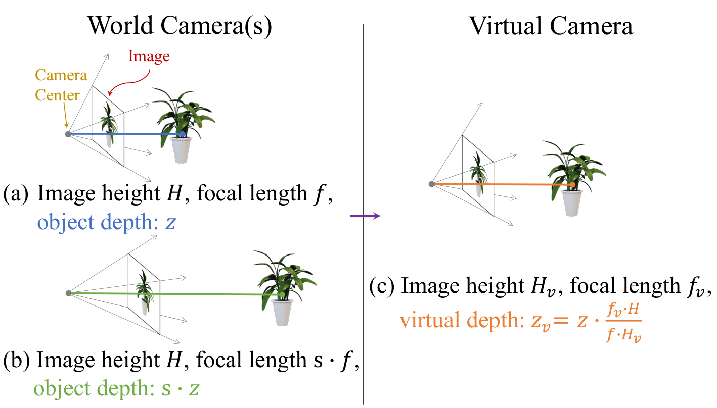
On the large and diverse Omni3D, we design a general and simple 3D object detector, called Cube R-CNN, inspired by advances in 2D and 3D recognition of recent years ren2015faster; simonelli2019disentangling; lu2021geometry; gkioxari2019mesh. Cube R-CNN detects all objects and their 3D location, size and rotation end-to-end from a single image of any domain and for many object categories. Attributed to Omni3D’s diversity, our model shows strong generalization and outperforms prior works for indoor and urban domains with one unified model, as shown in Fig. . Learning from such diverse data comes with challenges as Omni3D contains images of highly varying focal lengths which exaggerate scale-depth ambiguity (Fig. 3). We remedy this by operating on virtual depth which transforms object depth with the same virtual camera intrinsics across the dataset. An added benefit of virtual depth is that it allows the use of data augmentations (e.g. image rescaling) during training, which is a critical feature for 2D detection wu2019detectron2; mmdetection, and as we show, also for 3D. Our approach with one unified design outperforms prior best approaches in AP, ImVoxelNet rukhovich2022imvoxelnet by 4.1% on indoor SUN RGB-D, GUPNet lu2021geometry by 9.5% on urban KITTI, and PGD wang2022probabilistic by 7.9% on Omni3D.
We summarize our contributions:
- •
We introduce Omni3D, a benchmark for image-based 3D object detection sourced from existing 3D datasets, which is 20 larger than existing 3D benchmarks.
- •
We implement a new algorithm for IoU of 3D boxes, which is 450 faster than prior solutions.
- •
We design a general-purpose baseline method, Cube R-CNN, which tackles 3D object detection for many categories and across domains with a unified approach. We propose virtual depth to eliminate the ambiguity from varying camera focal lengths in Omni3D.
2 Related Work
Cube R-CNN and Omni3D draw from key research advances in 2D and 3D object detection.
2D Object Detection. Here, methods include two-stage approaches ren2015faster; he2017maskrcnn which predict object regions with a region proposal network (RPN) and then refine them via an MLP. Single-stage detectors redmon2016you; liu2016ssd; lin2017focal; zhou2019objects; tian2019fcos omit the RPN and predict regions directly from the backbone.
3D Object Detection. Monocular 3D object detectors predict 3D cuboids from single input images. There is extensive work in the urban self-driving domain where the car class is at the epicenter liu2021deep; reading2021categorical; chen2016monocular; mousavian20173d; liu2021ground; wang2021progressive; FuCVPR18DORN; gu2022homography; zhou2020iafa; ma2019accurate; he2021aug3d; simonelli2020towards; simonelli2019disentangling; huang2022monodtr; wang2021fcos3d. CenterNet zhou2019objects predicts 3D depth and size from fully-convolutional center features, and is extended by liu2020smoke; lu2021geometry; liu2021learning; zhang2021objects; zhou2021monocular; chen2020monopair; liu2021autoshape; li2020rtm3d; Ma_2021_CVPR; zhou2020iafa; kumar2022deviant. M3D-RPN brazil2019m3d trains an RPN with 3D anchors, enhanced further by ding2020learning; brazil2020kinematic; zou2021devil; wang2021depth; kumar2021groomed. FCOS3D wang2021fcos3d extends the anchorless FCOS tian2019fcos detector to predict 3D cuboids. Its successor PGD wang2022probabilistic furthers the approach with probabilistic depth uncertainty. Others use pseudo depth bao2019monofenet; you2019pseudo; wang2019pseudo; chen2022pseudo; park2021dd3d; Ma_2020_ECCV and explore depth and point-based LiDAR techniques qi2018frustum; ku2018joint. Similar to ours, chen2021monorun; simonelli2019disentangling; simonelli2020towards add a 3D head, specialized for urban scenes and objects, on two-stage Faster R-CNN. he2021aug3d; simonelli2020towards augment their training by synthetically generating depth and box-fitted views, coined as virtual views or depth. In our work, virtual depth aims at addressing varying focal lengths.
For indoor scenes, a vast line of work tackles room layout estimation hedau2009recovering; lee2009geometric; mallya2015learning; dasgupta2016delay. Huang et al huang2018cooperative predict 3D oriented bounding boxes for indoor objects. Factored3D factored3dTulsiani17 and 3D-RelNet kulkarni2019relnet jointly predict object voxel shapes. Total3D Nie_2020_CVPR predicts 3D boxes and meshes by additionally training on datasets with annotated 3D shapes. ImVoxelNet rukhovich2022imvoxelnet proposes domain-specific methods which share an underlying framework for processing volumes of 3D voxels. In contrast, we explore 3D object detection in its general form by tackling outdoor and indoor domains jointly in a single model and with a vocabulary of more categories.
3D Datasets. KITTI Geiger2012CVPR and SUN RGB-D song2015sun are popular datasets for 3D object detection on urban and indoor scenes respectively. Since 2019, 3D datasets have emerged, both for indoor objectron2021; hypersim; dehghan2021arkitscenes; dai2017scannet; avetisyan2019scan2cad and outdoor sun2020scalability; caesar2020nuscenes; houston2020one; chang2019argoverse; lyft; huang2019apolloscape; gahlert2020cityscapes. In isolation, these datasets target different tasks and applications and have unique properties and biases, e.g. object and scene types, focal length, coordinate systems, etc. In this work, we unify existing representative datasets Geiger2012CVPR; song2015sun; objectron2021; hypersim; dehghan2021arkitscenes; caesar2020nuscenes. We process the raw visual data, re-purpose their annotations, and carefully curate the union of their semantic labels in order to build a coherent large-scale benchmark, called Omni3D. Omni3D is larger than widely-used benchmarks and notably more diverse. As such, new challenges arise stemming from the increased variance in visual domain, object rotation, size, layouts, and camera intrinsics.
Omni3D SUN RGB-D KITTI COCO LVIS
 (a) Spatial statistics
(b) 2D Scale statistics
(c) Category statistics
(a) Spatial statistics
(b) 2D Scale statistics
(c) Category statistics
3 The Omni3D Benchmark
The primary benchmarks for 3D object detection are small, focus on a few categories and are of a single domain. For instance, the popular KITTI Geiger2012CVPR contains only urban scenes, has 7k images and 3 categories, with a focus on car. SUN RGB-D song2015sun has 10k images. The small size and lack of variance in 3D datasets is a stark difference to 2D counterparts, such as COCO lin2014microsoft and LVIS gupta2019lvis, which have pioneered progress in 2D recognition.
We aim to bridge the gap to 2D by introducing Omni3D, a large-scale and diverse benchmark for image-based 3D object detection consisting of 234k images, 3 million labeled 3D bounding boxes, and 98 object categories. We source from recently released 3D datasets of urban (nuScenes caesar2020nuscenes and KITTI Geiger2012CVPR), indoor (SUN RGB-D song2015sun, ARKitScenes dehghan2021arkitscenes and Hypersim hypersim), and general (Objectron objectron2021) scenes. Each of these datasets target different applications (e.g. point-cloud recognition or reconstruction in dehghan2021arkitscenes, inverse rendering in hypersim), provide visual data in different forms (e.g. videos in objectron2021; dehghan2021arkitscenes, rig captures in caesar2020nuscenes) and annotate different object types. To build a coherent benchmark, we process the varying raw visual data, re-purpose their annotations to extract 3D cuboids in a unified 3D camera coordinate system, and carefully curate the final vocabulary. More details about the benchmark creation in the Appendix.
We analyze Omni3D and show its rich spatial and semantic properties proving it is visually diverse, similar to 2D data, and highly challenging for 3D as depicted in Fig. 1. We show the value of Omni3D for the task of 3D object detection with extensive quantitative analysis in Sec. 5.
3.1 Dataset Analysis
Splits. We split the dataset into 175k/19k/39k images for train/val/test respectively, consistent with original splits when available, and otherwise free of overlapping video sequences in splits. We denote indoor and outdoor subsets as Omni3D (SUN RGB-D, Hypersim, ARKit), and Omni3D (KITTI, nuScenes). Objectron, with primarily close-up objects, is used only in the full Omni3D setting.
Layout statistics. Fig. 1(a) shows the distribution of object centers onto the image plane by projecting centroids on the XY-plane (top row), and the distribution of object depths by projecting centroids onto the XZ-plane (bottom row). We find that Omni3D’s spatial distribution has a center bias, similar to 2D datasets COCO and LVIS. Fig. 1(b) depicts the relative object size distribution, defined as the square root of object area divided by image area. Objects are more likely to be small in size similar to LVIS (Fig. 6c in gupta2019lvis) suggesting that Omni3D is also challenging for 2D detection, while objects in Omni3D are noticeably smaller.
The bottom row of Fig. 1(a) normalizes object depth in a range, chosen for visualization and satisfies of object instances; Omni3D depth ranges as far as m. We observe that the Omni3D depth distribution is far more diverse than SUN RGB-D and KITTI, which are biased toward near or road-side objects respectively. See Appendix for each data source distribution plot. Fig. 1(a) demonstrates Omni3D’s rich diversity in spatial distribution and depth which suffers significantly less bias than existing 3D benchmarks and is comparable in complexity to 2D datasets.
2D and 3D correlation. A common assumption in urban scenes is that objects rest on a ground plane and appear smaller with depth. To verify if that is true generally, we compute correlations. We find that 2D and 3D are indeed fairly correlated in Omni3D at , but significantly less in Omni3D at . Similarly, relative 2D object size () and correlation is and respectively. This confirms our claim that common assumptions in urban scenes are not generally true, making the task challenging.
Category statistics. Fig. 1(c) plots the distribution of instances across the 98 categories of Omni3D. The long-tail suggests that low-shot recognition in both 2D and 3D will be critical for performance. In this work, we want to focus on large-scale and diverse 3D recognition, which is comparably unexplored. We therefore filter and focus on categories with at least instances. This leaves 50 diverse categories including chair, sofa, laptop, table, books, car, truck, pedestrian and more, 19 of which have more than 10k instances. We provide more per-category details in the Appendix.

4 Method
Our goal is to design a simple and effective model for general 3D object detection. Hence, our approach is free of domain or object specific strategies. We design our 3D object detection framework by extending Faster R-CNN ren2015faster with a 3D object head which predicts a cuboid per each detected 2D object. We refer to our method as Cube R-CNN . Figure 2 shows an overview of our approach.
4.1 Cube R-CNN
Our model builds on Faster R-CNN ren2015faster, an end-to-end region-based object detection framework. Faster-RCNN consists of a backbone network, commonly a CNN, which embeds the input image into a higher-dimensional feature space. A region proposal network (RPN) predicts regions of interest (RoIs) representing object candidates in the image. A 2D box head inputs the backbone feature map and processes each RoI to predict a category and a more accurate 2D box. Faster R-CNN can be easily extended to tackle more tasks by adding task-specific heads, e.g. Mask R-CNN he2017maskrcnn adds a mask head to additionally output object silhouettes.
For the task of 3D object detection, we extend Faster R-CNN by introducing a 3D detection head which predicts a 3D cuboid for each detected 2D object. Cube R-CNN extends Faster R-CNN in three ways: (a) we replace the binary classifier in RPN which predicts region objectness with a regressor that predicts IoUness, (b) we introduce a cube head which estimates the parameters to define a 3D cuboid for each detected object (similar in concept to simonelli2019disentangling), and (c) we define a new training objective which incorporates a virtual depth for the task of 3D object detection.
IoUness. The role of RPN is two-fold: (a) it proposes RoIs by regressing 2D box coordinates from pre-computed anchors and (b) it classifies regions as object or not (objectness). This is sensible in exhaustively labeled datasets where it can be reliably assessed if a region contains an object. However, Omni3D combines many data sources with no guarantee that all instances of all classes are labeled. We overcome this by replacing objectness with IoUness, applied only to foreground. Similar to kim2022learning, a regressor predicts IoU between a RoI and a ground truth. Let be the predicted IoU for a RoI and be the 2D IoU between the region and its ground truth; we apply a binary cross-entropy (CE) loss . We train on regions whose IoU exceeds 0.05 with a ground truth in order to learn IoUness from a wide range of region overlaps. Thus, the RPN training objective becomes , where is the 2D box regression loss from ren2015faster. The loss is weighted by to prioritize candidates close to true objects.
Cube Head. We extend Faster R-CNN with a new head, called cube head, to predict a 3D cuboid for each detected 2D object. The cube head inputs feature maps pooled from the backbone for each predicted region and feeds them to fully-connected (FC) layers with hidden dimensions. All 3D estimations in the cube head are category-specific. The cube head represents a 3D cuboid with 13 parameters each predicted by a final FC layer:
- •
represent the projected 3D center on the image plane relative to the 2D RoI
- •
is the object’s center depth in meters transformed from virtual depth (explained below)
- •
are the log-normalized physical box dimensions in meters
- •
is the continuous 6D zhou2019continuity allocentric rotation
- •
is the predicted 3D uncertainty
The above parameters form the final 3D box in camera view coordinates for each detected 2D object. The object’s 3D center is estimated from the predicted 2D projected center and depth via
| (1) |
where is the object’s 2D box, are the camera’s known focal lengths and the principal point. The 3D box dimensions are derived from which are log-normalized with category-specific pre-computed means for width, height and length respectively, and are are arranged into a diagonal matrix via
| (2) |
Finally, we derive the object’s pose as a rotation matrix based on a 6D parameterization (2 directional vectors) of following zhou2019continuity which is converted from allocentric to egocentric rotation similar to kundu20183d, defined formally in Appendix. The final 3D cuboid, defined by corners, is
| (3) |
where are the 8 corners of an axis-aligned unit cube centered at . Lastly, denotes a learned 3D uncertainty, which is mapped to a confidence at inference then joined with the classification score from the 2D box head to form the final score for the prediction, as .
Training objective. Our training objective consists of 2D losses from the RPN and 2D box head and 3D losses from the cube head. The 3D objective compares each predicted 3D cuboid with its matched ground truth via a chamfer loss, treating the 8 box corners of the 3D boxes as point clouds, namely . Note that entangles all 3D variables via the box predictor (Eq. 3), such that that errors in variables may be ambiguous from one another. Thus, we isolate each variable group with separate disentangled losses, following simonelli2019disentangling. The disentangled loss for each variable group substitutes all but its variables with the ground truth from Eq. 3 to create a pseudo box prediction.For example, the disentangled loss for the projected center produces a 3D box with all but replaced with the true values and then compares to the ground truth box,
| (4) |
We use an loss for , and and chamfer for to account for cuboid symmetry such that rotation matrices of Euler angles modulo produce the same non-canonical 3D cuboid. Losses in box coordinates have natural advantages over losses which directly compare variables to ground truths in that their gradients are appropriately weighted by the error as shown in simonelli2019disentangling. The 3D objective is defined as, .
The collective training objective of Cube R-CNN is,
| (5) |
is the RPN loss, described above, and is the 2D box head loss from ren2015faster. The 3D loss is weighted by the predicted 3D uncertainty (inspired by lu2021geometry), such that the model may trade a penalty to reduce the 3D loss when uncertain. In practice, is helpful for both improving the 3D ratings at inference and reducing the loss of hard samples in training.
4.2 Virtual Depth
A critical part of 3D object detection is predicting an object’s depth in metric units. Estimating depth from visual cues requires an implicit mapping of 2D pixels to 3D distances, which is more ambiguous if camera intrinsics vary. Prior works are able to ignore this as they primarily train on images from a single sensor. Omni3D contains images from many sensors and thus demonstrates large variations in camera intrinsics. We design Cube R-CNN to be robust to intrinsics by predicting the object’s virtual depth , which projects the metric depth to an invariant camera space.
Virtual depth scales the depth using the (known) camera intrinsics such that the effective image size and focal length are consistent across the dataset, illustrated in Fig. 3. The effective image properties are referred to as virtual image height and virtual focal length , and are both hyperparameters. If is the true metric depth of an object from an image with height and focal length , its virtual depth is defined as . The derivation is in the Appendix.
Invariance to camera intrinsics via virtual depth also enables scale augmentations during training, since can vary without harming the consistency of . Data augmentations from image resizing tend to be critical for 2D models but are not often used in 3D methods brazil2019m3d; liu2020smoke; simonelli2019disentangling since if unaccounted for they increase scale-depth ambiguity. Virtual depth lessens such ambiguities and therefore enables powerful data augmentations in training. We empirically prove the two-fold effects of virtual depth in Sec. 5

5 Experiments
We tackle image-based 3D object detection on Omni3D and compare to prior best methods. We evaluate Cube R-CNN on existing 3D benchmarks with a single unified model. Finally, we prove the effectiveness of Omni3D as a large-scale 3D object detection dataset by showing comprehensive cross-dataset generalization and its impact for pre-training.
Implementation details. We implement Cube R-CNN using Detectron2 wu2019detectron2 and PyTorch3D ravi2020pytorch3d. Our backbone is DLA34 yu2018deep-FPN lin2017feature pretrained on ImageNet russakovsky2015imagenet. We train for 128 epochs with a batch size of 192 images across 48 V100s. We use SGD with a learning rate of 0.12 which decays by a factor of 10 after 60% and 80% of training. During training, we use random data augmentation of horizontal flipping and scales , enabled by virtual depth. Virtual camera parameters are set to . Source code and models are publicly available.
Metric. Following popular benchmarks for 2D and 3D recognition, we use average-precision (AP) as our 3D metric. Predictions are matched to ground truth by measuring their overlap using which computes the intersection-over-union of 3D cuboids. We compute a mean AP across all 50 categories in Omni3D and over a range of thresholds . The range of is more relaxed than in 2D to account for the new dimension – see the Appendix for a comparison between 3D and 2D ranges for IoU. General 3D objects may be occluded by other objects or truncated by the image border, and can have arbitrarily small projections. Following Geiger2012CVPR, we ignore objects with high occlusion () or truncation (), and tiny projected objects ( image height). Moreover, we also report AP at varying levels of depth as near: , medium: , far: .
Fast . compares two 3D cuboids by computing their intersection-over-union. Images usually have many objects and produce several predictions so computations need to be fast. Prior implementations Geiger2012CVPR approximate by projecting 3D boxes on a ground plane and multiply the top-view 2D intersection with the box heights to compute a 3D volume. Such approximations become notably inaccurate when objects are not on a planar ground or have an arbitrary orientation (e.g. with nonzero pitch or roll).Objectron objectron2021 provides an exact solution, but relies on external libraries virtanen2020scipy; barber1996quickhull implemented in C++ and is not batched. We implement a new, fast and exact algorithm which computes the intersecting shape by representing cuboids as meshes and finds face intersections – described in Appendix. Our algorithm is batched with C++ and CUDA support. Our implementation is faster than Objectron in C++, and faster in CUDA. As a result, evaluation on the large Omni3D takes only seconds instead of several hours.
5.1 Model Performance
First, we ablate the design choices of Cube R-CNN. Then, we compare to state-of-the-art methods on existing benchmarks and Omni3D and show that it performs superior or on par with prior works which are specialized for their respective domains. Our Cube R-CNN uses a single unified design to tackle general 3D object detection across domains. Fig. 4 shows qualitative predictions on the Omni3D test set.
| Cube R-CNN | AP | AP | AP | AP | AP | AP | AP | AP |
| w/o disentangled | 22.6 | 24.3 | 9.2 | 26.8 | 11.8 | 8.2 | 14.5 | 30.9 |
| w/o IoUness | 22.2 | 23.6 | 8.8 | 26.4 | 11.1 | 8.3 | 14.3 | 31.0 |
| w/o | 20.2 | 21.8 | 6.4 | 26.4 | 12.1 | 7.4 | 13.8 | 29.1 |
| w/o scale aug. | 20.2 | 21.5 | 8.0 | 23.5 | 9.8 | 6.8 | 12.3 | 28.1 |
| w/o scale virtual | 19.8 | 21.2 | 7.5 | 23.4 | 8.6 | 5.7 | 12.2 | 26.0 |
| w/o virtual depth | 17.3 | 18.4 | 4.4 | 22.7 | 7.9 | 7.1 | 13.2 | 30.3 |
| w/o uncertainty | 17.2 | 18.3 | 5.4 | 20.5 | 10.8 | 7.0 | 9.1 | 25.4 |
| ours | 23.3 | 24.9 | 9.5 | 27.9 | 12.1 | 8.5 | 15.0 | 31.9 |
| Omni3D | Omni3D | ||||
| Method | AP | AP | AP | AP | |
| M3D-RPN brazil2019m3d | ✗ | 10.4 | 17.9 | 13.7 | - |
| SMOKE liu2020smoke | ✗ | 25.4 | 20.4 | 19.5 | 9.6 |
| FCOS3D wang2021fcos3d | ✗ | 14.6 | 20.9 | 17.6 | 9.8 |
| PGD wang2022probabilistic | ✗ | 21.4 | 26.3 | 22.9 | 11.2 |
| GUPNet lu2021geometry | ✓ | 24.5 | 20.5 | 19.9 | - |
| M3D-RPN +vc | ✓ | 16.2+5.8 | 20.4+2.9 | 17.0+3.3 | - |
| ImVoxelNet rukhovich2022imvoxelnet | ✓ | 23.5 | 23.4 | 21.5 | 9.4 |
| SMOKE +vc | ✓ | 25.9+0.5 | 20.4+0.0 | 20.0+0.5 | 10.4+0.8 |
| FCOS3D +vc | ✓ | 17.8+3.2 | 25.1+4.2 | 21.3+3.7 | 10.6+0.8 |
| PGD +vc | ✓ | 22.8+1.4 | 31.2+4.9 | 26.8+3.9 | 15.4+4.2 |
| Cube R-CNN | ✓ | 36.0 | 32.7 | 31.9 | 23.3 |
Ablations. Table 1 ablates the features of Cube R-CNN on Omni3D. We report AP, performance at single IoU thresholds (0.25 and 0.50), and for near, medium and far objects. We further train and evaluate on domain-specific subsets, Omni3D (AP) and Omni3D (AP) to show how ablation trends hold for single domain scenarios. From Table 1 we draw a few standout observations:
Virtual depth is effective and improves AP by %, most noticable in the full Omni3D which has the largest variances in camera intrinsics. Enabled by virtual depth, scale augmentations during training increase AP by % on Omni3D, % on Omni3D and % on Omni3D. We find scale augmentation controlled without virtual depth to be harmful by (rows 6 - 7).
3D uncertainty boosts performance by about % on all Omni3D subsets. Intuitively, it serves as a measure of confidence for the model’s 3D predictions; removing it means that the model relies only on its 2D classification to score cuboids. If uncertainty is used only to scale samples in Eq. 5, but not at inference then AP still improves but by .
Table 1 also shows that the entangled loss from Eq. 5 boosts AP by % while disentangled losses contribute less (%). Replacing objectness with IoUness in the RPN head improves AP on Omni3D by %.
Comparison to other methods. We compare Cube R-CNN to prior best approaches. We choose representative state-of-the-art methods designed for the urban and indoor domains, and evaluate on our proposed Omni3D benchmark and single-dataset benchmarks, KITTI and SUN RGB-D.
Comparisons on Omni3D. Table 2 compares Cube R-CNN to M3D-RPN brazil2019m3d, a single-shot 3D anchor approach, FCOS3D wang2021fcos3d and its follow-up PGD wang2022probabilistic, which use a fully convolutional one-stage model, GUPNet lu2021geometry, which uses 2D-3D geometry and camera focal length to derive depth, SMOKE liu2020smoke which predicts 3D object center and offsets densely and ImVoxelNet rukhovich2022imvoxelnet, which uses intrinsics to unproject 2D image features to a 3D volume followed by 3D convolutions. These methods originally experiment on urban domains, so we compare on Omni3D and the full Omni3D. We train each method using public code and report the best of multiple runs after tuning their hyper-parameters to ensure best performance. We extend all but GUPNet and ImVoxelNet with a virtual camera to handle varying intrinsics, denoted by +vc. GUPNet and ImVoxelNet dynamically use per-image intrinsics, which can naturally account for camera variation. M3D-RPN and GUPNet do not support multi-node training, which makes scaling to Omni3D difficult and are omitted. For Omni3D, we report AP on its test set and its subparts, AP and AP.
From Table 2 we observe that our Cube R-CNN outperforms competitive methods on both Omni3D and Omni3D. The virtual camera extensions result in performance gains of varying degree for all approaches, e.g. for PGD on Omni3D, proving its impact as a general purpose feature for mixed dataset training for the task of 3D object detection. FCOS3D, SMOKE, and ImVoxelNet rukhovich2022imvoxelnet struggle the most on Omni3D, which is not surprising as they are typically tailored for dataset-specific model choices.
| AP | AP | ||||||
| Method | D | Easy | Med | Hard | Easy | Med | Hard |
| SMOKE liu2020smoke | ✗ | 14.03 | 9.76 | 7.84 | 20.83 | 14.49 | 12.75 |
| ImVoxelNet rukhovich2022imvoxelnet | ✗ | 17.15 | 10.97 | 9.15 | 25.19 | 16.37 | 13.58 |
| PGD wang2022probabilistic | ✗ | 19.05 | 11.76 | 9.39 | 26.89 | 16.51 | 13.49 |
| GUPNet lu2021geometry | ✗ | 22.26 | 15.02 | 13.12 | 30.29 | 21.19 | 18.20 |
| Cube R-CNN | ✗ | 23.59 | 15.01 | 12.56 | 31.70 | 21.20 | 18.43 |
| MonoDTR huang2022monodtr | ✓ | 21.99 | 15.39 | 12.73 | 28.59 | 20.38 | 17.14 |
| DD3D park2021dd3d | ✓ | 23.19 | 16.87 | 14.36 | 32.35 | 23.41 | 20.42 |
Comparisons on KITTI. Table 3 shows results on KITTI’s test set using their server kittiserver. We train Cube R-CNN on KITTI only. Cube R-CNN is a general purpose 3D object detector; its design is not tuned for the KITTI benchmark. Yet, it performs better or on par with recent best methods which are heavily tailored for KITTI and is only slightly worse to models trained with extra depth supervision.
| Method | Trained on | AP | |
| Total3D Nie_2020_CVPR | SUN RGB-D | 23.3 | - |
| ImVoxelNet rukhovich2022imvoxelnet | SUN RGB-D | - | 30.6 |
| Cube R-CNN | SUN RGB-D | 36.2 | 34.7 |
| Cube R-CNN | Omni3D | 37.8 | 35.4 |
KITTI’s AP is fundamentally similar to ours but sets a single threshold at 0.70, which behaves similar to a nearly perfect 2D threshold of 0.94 (see the Appendix). To remedy this, our AP is a mean over many thresholds, inspired by COCO lin2014microsoft. In contrast, nuScenes proposes a mean AP based on 3D center distance but omits size and rotation, with settings generally tailored to the urban domain (e.g. size and rotation variations are less extreme for cars). We provide more analysis with this metric in the Appendix.
Comparisons on SUN RGB-D. Table 4 compares Cube R-CNN to Total3D Nie_2020_CVPR and ImVoxelNet rukhovich2022imvoxelnet, two state-of-the-art methods on SUN RGB-D on 10 common categories. Total3D’s public model requires 2D object boxes and categories as input. Hence, for a fair comparison, we use ground truth 2D detections as input to both our and their method, each trained using a ResNet34 he2016deep backbone and report mean (3 col). We compare to ImVoxelNet in the full 3D object detection setting and report AP (4 col). We compare Cube R-CNN from two respects, first trained on SUN RGB-D identical to the baselines, then trained on Omni3D which subsumes SUN RGB-D. Our model outperforms Total3D by and ImVoxelNet by when trained on the same training set and increases the performance gap when trained on the larger Omni3D.
Zero-shot Performance. One commonly sought after property of detectors is zero-shot generalization to other datasets. Cube R-CNN outperforms all other methods at zero-shot. We find our model trained on KITTI achieves 12.7% AP on nuScenes; the second best is M3D-RPN+vc with 10.7%. Conversely, when training on nuScenes, our model achieves 20.2% on KITTI; the second best is GUPNet with 17.3%.
5.2 The Impact of the Omni3D Benchmark
Sec. 5.1 analyzes the performance of Cube R-CNN for the task of 3D object detection. Now, we turn to Omni3D and its impact as a large-scale benchmark. We show two use cases of Omni3D: (a) a universal 3D dataset which integrates smaller ones, and (b) a pre-training dataset.
Omni3D as a universal dataset. We treat Omni3D as a dataset which integrates smaller single ones and show its impact on each one. We train Cube R-CNN on Omni3D and compare to single-dataset training in Table 5, for the indoor (left) and urban (right) domain. AP is reported on the category intersection (10 for indoor, 3 for outdoor) to ensure comparability. Training on Omni3D and its domain-specific subsets, Omni3D and Omni3D, results in higher performance compared to single-dataset training, signifying that our large Omni3D generalizes better and should be preferred over single dataset training. ARKit sees a boost and KITTI %. Except for Hypersim, the domain-specific subsets tend to perform better on their domain, which is not surprising given their distinct properties (Fig. 1).
Omni3D as a pre-training dataset. Next, we demonstrate the utility of Omni3D for pre-training. In this setting, an unseen dataset is used for finetuning from a model pre-trained on Omni3D. The motivation is to determine how a large-scale 3D dataset could accelerate low-shot learning with minimum need for costly 3D annotations on a new dataset. We choose SUN RGB-D and KITTI as our unseen datasets given their popularity and small size. We pre-train Cube R-CNN on Omni3D-, which removes them from Omni3D, then finetune the models using a % of their training data. The curves in Fig. 5 show the model quickly gains its upper-bound performance at a small fraction of the training data, when pre-trained on Omni3D- vs. ImageNet, without any few-shot training tricks. A model finetuned on only 5% of its target can achieve 70% of the upper-bound performance.
| Trained on | AP | AP | AP |
| Hypersim | 15.2 | 9.5 | 7.5 |
| SUN | 5.8 | 34.7 | 13.1 |
| ARKit | 5.9 | 14.2 | 38.6 |
| Omni3D | 19.0 | 32.6 | 38.2 |
| Omni3D | 17.8 | 35.4 | 41.2 |
| Trained on | AP | AP |
| KITTI | 37.1 | 12.7 |
| nuScenes | 20.2 | 38.6 |
| Omni3D | 37.8 | 35.8 |
| Omni3D | 42.4 | 39.0 |
![[Uncaptioned image]](2207.10660v2/figures/AP_over_percent_sun.jpg)
![[Uncaptioned image]](2207.10660v2/figures/AP_over_percent_kit.jpg)
Omni3D Omni3D Omni3D SUN RGB-D ARKit Hypersim Objectron KITTI nuScenes COCO LVIS

6 Conclusion
We propose a large and diverse 3D object detection benchmark, Omni3D, and a general purpose 3D object detector, Cube R-CNN. Models and data are publicly released. Our extensive analysis (Table 1, Fig. 4, Appendix) show the strength of general 3D object detection as well as the limitations of our method, e.g. localizing far away objects, and uncommon object types or contexts. Moreover, for accurate real-world 3D predictions, our method is limited by the assumption of known camera intrinsics, which may be minimized in future work using self-calibration techniques.
Appendix
A1 Dataset Details
In this section, we provide details related to the creation of Omni3D, its sources, coordinate systems, and statistics.
Sources. For each individual dataset used in Omni3D, we use their official train, val, and test set for any datasets which have all annotations released. If no public test set is available then we use their validation set as our test set. Whenever necessary we further split the remaining training set in 10:1 ratio by sequences in order form train and val sets. The resultant image make up of Omni3D is detailed in Table 6. To make the benchmark coherent we merged semantic categories across the sources, e.g., there are 26 variants of chair including ‘chair’, ‘chairs’, ‘recliner’, ‘rocking chair’, etc. We show the category instance counts in Figure 7.
Coordinate system. We define our unified 3D coordinate system for all labels with the camera center being the origin and +x facing right, +y facing down, +z inward Geiger2012CVPR. Object pose is relative to an initial object with its bottom-face normal aligned to +y and its front-face aligned to +x (e.g. upright and facing to the right). All images have known camera calibration matrices with input resolutions varying from to and diverse focal lengths from to in pixels. Each object label contains a category label, a 2D bounding box, a 3D centroid in camera space meters, a matrix defining the object to camera rotation, and the physical dimensions (width, height, length) in meters.
Spatial Statistics. Following Section 3 of the main paper, we provide the spatial statistics for the individual data sources of SUN RGB-D song2015sun, ARKit dehghan2021arkitscenes, Hypersim hypersim, Objectron objectron2021, KITTI Geiger2012CVPR, nuScenes caesar2020nuscenes, as well as Omni3D and Omni3D in Figure 6. As we mention in the main paper, we observe that the indoor domain data, with the exception of Hypersim, have bias for close objects. Moreover, outdoor data tend to be spatially biased with projected centroids along diagonal ground planes while indoor is more central. We provide a more detailed view of density-normalized depth distributions for each dataset in Figure 8.
| Method | Total | Train | Val | Test | ||
| KITTI Geiger2012CVPR | 8 | 5 | 7,481 | 3,321 | 391 | 3,769 |
| SUN RGB-D song2015sun | 83 | 38 | 10,335 | 4,929 | 356 | 5,050 |
| nuScenes caesar2020nuscenes | 9 | 9 | 34,149 | 26,215 | 1,915 | 6,019 |
| Objectron objectron2021 | 9 | 9 | 46,644 | 33,519 | 3,811 | 9,314 |
| ARKitScenes dehghan2021arkitscenes | 15 | 14 | 60,924 | 48,046 | 5,268 | 7,610 |
| Hypersim hypersim | 32 | 29 | 74,619 | 59,543 | 7,386 | 7,690 |
| Omni3D | 14 | 11 | 41,630 | 29,536 | 2,306 | 9,788 |
| Omni3D | 84 | 38 | 145,878 | 112,518 | 13,010 | 20,350 |
| Omni3D | 98 | 50 | 234,152 | 175,573 | 19,127 | 39,452 |


A2 Model Details
In this section, we provide more details for Cube R-CNN pertaining to its 3D bounding box allocentric rotation (Sec. 4.1) and the derivation of virtual depth (Sec. 4.2).
A2.1 3D Box Rotation
Our 3D bounding box object rotation is predicted in the form of a 6D continuous parameter, which is shown in zhou2019continuity to be better suited for neural networks to regress compared to other forms of rotation. Let our predicted rotation be split into two directional vectors and be the columns of a rotational matrix . Then is mapped to via
| (6) | ||||
| (7) | ||||
| (8) |
where denote dot and cross product respectively.
is estimated in allocentric form similar to kundu20183d. Let be the known camera intrinsics, the predicted 2D projected center as in Section 4.1, and be the camera’s principal axis. Then is a ray pointing from the camera to with angle . Using standard practices of axis angle representations with an axis denoted as and angle , we compute a matrix , which helps form the final egocentric rotation matrix .
We provide examples of 3D bounding boxes at constant egocentric or allocentric rotations in Figure 9. The allocentric rotation is more aligned to the visual 2D evidence, whereas egocentric rotation entangles relative position into the prediction. In other words, identical egocentric rotations may look very different when viewed from varying spatial locations, which is not true for allocentric.
A2.2 Virtual Depth
In Section 4.2, we propose a virtual depth transformation in order to help Cube R-CNN handle varying input image resolutions and camera intrinsics. In our experiments, we show that virtual depth also helps other competing approaches, proving its effectiveness as a general purpose feature. The motivation of estimating a virtual depth instead of metric depth is to keep the effective image size and focal length consistent in an invariant camera space. Doing so enables two camera systems with nearly the same visual evidence of an object to transform into the same virtual depth as shown in Figure 4 of the main paper. Next we provide the proof for the conversion between virtual and metric depth.
Proof: Assume a 3D point projected to on an image with height and focal length .The virtual 3D point is projected to on the virtual image. The 2D points and correspond to the same pixel location in both the original and virtual image. In other words, . Recall the formula for projection as and , where is the principal point and . By substitution .
A2.3 Training Details and Efficiency
When training on subsets smaller than Omni3D, we adjust the learning rate, batch size, and number of iterations linearly until we can train for 128 epochs between 96k to 116k iterations. Cube R-CNN trains on V100 GPUs between 14 and 26 hours depending on the subset configuration when scaled to multi-node distributed training, and while training uses approximately 1.6 GB memory per image. Inference on a Cube R-CNN model processes image from KITTI Geiger2012CVPR with a wide input resolution of 5121696 at 52ms/image on average while taking up 1.3 GB memory on a Quadro GP100 GPU. Computed with an identical environment, our model efficiency is favorable to M3D-RPN brazil2019m3d and GUPNet lu2021geometry which infer from KITTI images at 191ms and 66ms on average, respectively.
A3 Evaluation
In this section we give additional context and justification for our chosen thresholds which define the ranges of 3D IoU that AP is averaged over. We further provide details on our implementation of 3D IoU.

A3.1 Thresholds for AP
We highlight the relationship between 2D and 3D IoU in Figure 10. We do so by contriving a general example between a ground truth and a predicted box, both of which share rotation and rectangular cuboid dimensions (). We then translate the 3D box along the -axis up to 1 meter (its unit length), simulating small to large errors in depth estimation. As shown in the left of Figure 10, the 3D IoU drops off significantly quicker than 2D IoU does between the projected 2D bounding boxes. As visualized in right of Figure 10, a moderate score of 0.63 IoU may result in a low IoU. Despite visually appearing to be well localized in the front view, the top view helps reveal the error. Since depth is a key error mode for 3D, we find the relaxed settings of compared to 2D (Sec. 5) to be reasonable.
A3.2 Details
We implement a fast . We provide more details for our algorithm here. Our algorithm starts from the simple observation that the intersection of two oriented 3D boxes, and , is a convex polyhedron with comprised of connected planar units. In 3D, these planar units are 3D triangular faces. Critically, each planar unit belongs strictly to either or . Our algorithm finds these units by iterating through the sides of each box, as described in Algorithm 1.
Step 2: If is not inside, then we discard it
Step 3: If is inside, then . If is partially inside, then the part of inside , call it , is added to ,
Step 4: We repeat steps 1 - 3 for
Step 5: We check and remove duplicates in (in the case of coplanar sides in and )
Step 6: We compute the volume of , which is guaranteed to be convex
A4 nuScenes Performance
In the main paper, we compare Cube R-CNN to competing methods with the popular IoU-based AP metric, which is commonly used and suitable for general purpose 3D object detection. Here, we additionally compare our Cube R-CNN to best performing methods with the nuScenes evaluation metric, which is designed for the urban domain. The released nuScenes dataset has 6 cameras in total and reports custom designed metrics of mAP and NDS as detailed in caesar2020nuscenes. Predictions from the 6 input views (each from a different camera) are fused to produce a single prediction. In contrast, our benchmark uses 1 camera (front) and therefore does not require or involve any post-processing fusion nor any dataset-specific predictions (e.g velocity and attributes). Moreover, as discussed in Section 5.1, the mAP score used in nuScenes is based on distances of 3D object centers which ignores errors in rotation and object dimensions. This is suited for urban domains as cars tend to vary less in size and orientation and is partially addressed in the NDS metric where true-positive (TP) metrics are factored in as an average over mAP and TP (Eq. 3 of caesar2020nuscenes).
| nuScenes Front Camera Only | |||||||
| Method | TTA | mAP | mATE | mASE | mAOE | NDS | AP |
| FCOS3D wang2021fcos3d | ✓ | 35.3 | 0.777 | 0.231 | 0.400 | 44.2 | 27.9 |
| PGD wang2022probabilistic | ✓ | 39.0 | 0.675 | 0.236 | 0.399 | 47.6 | 32.3 |
| Cube R-CNN | ✗ | 32.6 | 0.671 | 0.289 | 1.000 | 33.6 | 33.0 |
We compare with the current best performing methods on nuScenes, FCOS3D wang2021fcos3d and PGD wang2022probabilistic. We take their best models including fine-tuning and test-time augmentations (TTA), then modify the nuScenes evaluation metric in the following three ways:
- 1.
We evaluate on the single front camera setting.
- 2.
We merge the construction vehicle and truck categories, as in the pre-processing of Omni3D.
- 3.
We drop the velocity and attribute true-positive metrics from being included in the NDS metric. Following caesar2020nuscenes our TP {mATE, mASE, mAOE} resulting in a metric of
Table 7 reports the performance of each nuScenes metric for Cube R-CNN, FCOS3D, and PGD along with our AP. Since these methods are evaluated on the front cameras, no late-fusion of the full camera array is performed and side/back camera ground truths are not evaluated with. Cube R-CNN performs competitively but slightly worse on the mAP center-distance metric compared to FCOS3D and PGD. This is not surprising as the FCOS3D and PGD models were tuned for the nuScenes benchmark and metric and additionally use test time augmentations, while we don’t.
| Method | Trained on | table | bed | sofa | bathtub | sink | shelves | cabinet | fridge | chair | television | avg. |
| ImVoxelNet rukhovich2022imvoxelnet | SUN RGB-D | 39.5 | 68.8 | 48.9 | 33.9 | 18.7 | 2.4 | 13.2 | 17.0 | 55.5 | 8.4 | 30.6 |
| Cube R-CNN | SUN RGB-D | 39.2 | 65.7 | 58.1 | 49.0 | 32.5 | 4.3 | 16.2 | 25.2 | 54.5 | 2.7 | 34.7 |
| Cube R-CNN | Omni3D | 38.3 | 66.5 | 60.3 | 51.8 | 30.8 | 3.2 | 13.3 | 30.3 | 56.1 | 3.6 | 35.4 |
| Method | Trained on | table | bed | sofa | bathtub | sink | shelves | cabinet | fridge | chair | toilet | avg. |
| Total3D Nie_2020_CVPR | SUN RGB-D | 27.7 | 33.6 | 30.1 | 28.5 | 18.8 | 10.1 | 13.1 | 19.1 | 24.2 | 28.1 | 23.3 |
| Cube R-CNN | SUN RGB-D | 39.2 | 49.5 | 46.0 | 32.2 | 31.9 | 16.2 | 26.5 | 34.7 | 39.9 | 45.7 | 36.2 |
| Cube R-CNN | Omni3D | 40.7 | 50.1 | 50.0 | 33.8 | 31.8 | 18.2 | 29.0 | 34.6 | 41.6 | 48.2 | 37.8 |
A5 Full Category Performance on Omni3D
We train Cube R-CNN on the full categories within Omni3D, in contrast to the main paper which uses the most frequent categories with more than positive instances. As expected, the AP performance decreases when evaluating on the full categories from to , and similarly for AP from to . At the long-tails, we expect 2D and 3D object recognition will suffer since fewer positive examples are available for learning. We expect techniques related to few-shot recognition could be impactful and lend to a new avenue for exploration with Omni3D.
A6 Per-category SUN RGB-D Performance
We show per-category performance on AP for Cube R-CNN and ImVoxelNet rukhovich2022imvoxelnet’s publicly released indoor model in Table 8. We show the 10 common categories which intersect all indoor datasets as used in Table 4-5 in the main paper for fair comparisons when training categories differ.
Similarly, Table 9 shows detailed per-category performance for Cube R-CNN and Total3D Nie_2020_CVPR on 10 common categories, a summary of which was presented in Table 4 in the main paper. Note that television, in our 10 intersecting categories, is not detected by Total3D thus we replace it by toilet which is the next most common category.
A7 Regarding the Public Models Used for Omni3D Comparisons
We use publicly released code for M3D-RPN brazil2019m3d, GUPNet lu2021geometry, SMOKE liu2020smoke, FCOS3D wang2021fcos3d, PGD wang2022probabilistic, and ImVoxelNet rukhovich2022imvoxelnet and Total3D Nie_2020_CVPR in Section 5. Most of these models are implemented in the mmdetection3d mmdet3d2020 open-source repository, which critically supports many features for dataset scaling such as distributed scaling and strategic data sampling.
Most of the above methods tailor their configuration hyper-parameters in a handful of ways specifically for each dataset they were originally designed for. Since our experiments explicitly run on mixed datasets which have diverse resolutions, aspect ratios, depth distributions, etc., we opted to run each method on a variety of settings. We did our best to run each method on multiple sensible hyper-parameters settings to give each method the most fair chance. We focused primarily on the settings which are impacted by input resolution and depth distributions, as these are seemingly the biggest distinctions between datasets. When applicable, we implemented virtual depth with a custom design for each method depending on its code structure (see main paper).
Although we expect that better recipes can be found for each method, we ran more than 100 experiments and are using 17 of these runs selected based on best performance to report in the paper.
A8 Qualitative Examples
Figure 11 shows more Cube R-CNN predictions on Omni3D test. In Figure 12, we demonstrate generalization for interesting scenes in the wild from COCO lin2014microsoft images. When projecting on images with unknown camera intrinsics, as is the case for COCO, we visualize with intrinsics of , where is the input image resolution. As shown in Figure 12, this appears to result in fairly stable generalization for indoor and more common failure cases concerning unseen object or camera poses in outdoor. We note that simple assumptions of intrinsics prevent our 3D localization predictions from being real-world up to a scaling factor. This could be resolved using either real intrinsics or partially handled via image-based self-calibration hemayed2003survey; itu2020self; zhuang2019degeneracy which is itself a challenging problem in computer vision.
Lastly, we provide a demo video22 2 https://omni3d.garrickbrazil.com/#demo which further demonstrates Cube R-CNN’s generalization when trained on Omni3D and then applied to in the wild video scenes from a headset mounted camera, similar to AR/VR heasets. In the video, we apply a simple tracking algorithm which merges predictions in 3D space using 3D IoU and category cosine similarity when comparing boxes. We show the image-based boxes on the left and a static view of the room on the right. We emphasize that this video demonstrates zero-shot performance since no fine-tuning was done on the domain data.


References
- (1) KITTI server. https://www.cvlibs.net/datasets/kitti/eval_object.php?obj_benchmark=3d. Accessed: 2022-11-01.
- (2) Adel Ahmadyan, Liangkai Zhang, Artsiom Ablavatski, Jianing Wei, and Matthias Grundmann. Objectron: A large scale dataset of object-centric videos in the wild with pose annotations. CVPR, 2021.
- (3) Armen Avetisyan, Manuel Dahnert, Angela Dai, Manolis Savva, Angel X Chang, and Matthias Nießner. Scan2CAD: Learning CAD model alignment in RGB-D scans. In Proceedings of the IEEE/CVF Conference on computer vision and pattern recognition, pages 2614–2623, 2019.
- (4) Wentao Bao, Bin Xu, and Zhenzhong Chen. MonoFENet: Monocular 3D object detection with feature enhancement networks. TIP, 2019.
- (5) Bradford Barber, David Dobkin, and Hannu Huhdanpaa. The quickhull algorithm for convex hulls. ACM Transactions on Mathematical Software (TOMS), 1996.
- (6) Gilad Baruch, Zhuoyuan Chen, Afshin Dehghan, Tal Dimry, Yuri Feigin, Peter Fu, Thomas Gebauer, Brandon Joffe, Daniel Kurz, Arik Schwartz, and Elad Shulman. ARKitScenes - a diverse real-world dataset for 3D indoor scene understanding using mobile RGB-D data. In NeurIPS Datasets and Benchmarks Track, 2021.
- (7) Garrick Brazil and Xiaoming Liu. M3D-RPN: Monocular 3D region proposal network for object detection. In ICCV, 2019.
- (8) Garrick Brazil, Gerard Pons-Moll, Xiaoming Liu, and Bernt Schiele. Kinematic 3D object detection in monocular video. In ECCV, 2020.
- (9) Holger Caesar, Varun Bankiti, Alex H Lang, Sourabh Vora, Venice Erin Liong, Qiang Xu, Anush Krishnan, Yu Pan, Giancarlo Baldan, and Oscar Beijbom. nuScenes: A multimodal dataset for autonomous driving. In CVPR, 2020.
- (10) Ming-Fang Chang, John Lambert, Patsorn Sangkloy, Jagjeet Singh, Slawomir Bak, Andrew Hartnett, De Wang, Peter Carr, Simon Lucey, Deva Ramanan, et al. Argoverse: 3D tracking and forecasting with rich maps. In CVPR, 2019.
- (11) Hansheng Chen, Yuyao Huang, Wei Tian, Zhong Gao, and Lu Xiong. MonoRUn: Monocular 3D object detection by reconstruction and uncertainty propagation. In CVPR, 2021.
- (12) Kai Chen, Jiaqi Wang, Jiangmiao Pang, Yuhang Cao, Yu Xiong, Xiaoxiao Li, Shuyang Sun, Wansen Feng, Ziwei Liu, Jiarui Xu, Zheng Zhang, Dazhi Cheng, Chenchen Zhu, Tianheng Cheng, Qijie Zhao, Buyu Li, Xin Lu, Rui Zhu, Yue Wu, Jifeng Dai, Jingdong Wang, Jianping Shi, Wanli Ouyang, Chen Change Loy, and Dahua Lin. MMDetection: Open mmlab detection toolbox and benchmark. arXiv preprint arXiv:1906.07155, 2019.
- (13) Xiaozhi Chen, Kaustav Kundu, Ziyu Zhang, Huimin Ma, Sanja Fidler, and Raquel Urtasun. Monocular 3D object detection for autonomous driving. In CVPR, 2016.
- (14) Yongjian Chen, Lei Tai, Kai Sun, and Mingyang Li. MonoPair: Monocular 3D object detection using pairwise spatial relationships. In CVPR, 2020.
- (15) Yi-Nan Chen, Hang Dai, and Yong Ding. Pseudo-stereo for monocular 3D object detection in autonomous driving. In CVPR, 2022.
- (16) MMDetection3D Contributors. MMDetection3D: OpenMMLab next-generation platform for general 3D object detection. https://github.com/open-mmlab/mmdetection3d, 2020.
- (17) Angela Dai, Angel X. Chang, Manolis Savva, Maciej Halber, Thomas Funkhouser, and Matthias Nießner. ScanNet: Richly-annotated 3D reconstructions of indoor scenes. In CVPR, 2017.
- (18) Saumitro Dasgupta, Kuan Fang, Kevin Chen, and Silvio Savarese. Delay: Robust spatial layout estimation for cluttered indoor scenes. In CVPR, 2016.
- (19) Mingyu Ding, Yuqi Huo, Hongwei Yi, Zhe Wang, Jianping Shi, Zhiwu Lu, and Ping Luo. Learning depth-guided convolutions for monocular 3D object detection. In CVPRW, 2020.
- (20) Huan Fu, Mingming Gong, Chaohui Wang, Kayhan Batmanghelich, and Dacheng Tao. Deep Ordinal Regression Network for Monocular Depth Estimation. In CVPR, 2018.
- (21) Nils Gählert, Nicolas Jourdan, Marius Cordts, Uwe Franke, and Joachim Denzler. Cityscapes 3D: Dataset and benchmark for 9 DOF vehicle detection. In CVPRW, 2020.
- (22) Andreas Geiger, Philip Lenz, and Raquel Urtasun. Are we ready for autonomous driving? the KITTI vision benchmark suite. In CVPR, 2012.
- (23) Georgia Gkioxari, Jitendra Malik, and Justin Johnson. Mesh R-CNN. In ICCV, 2019.
- (24) Jiaqi Gu, Bojian Wu, Lubin Fan, Jianqiang Huang, Shen Cao, Zhiyu Xiang, and Xian-Sheng Hua. Homography loss for monocular 3D object detection. In CVPR, 2022.
- (25) Agrim Gupta, Piotr Dollar, and Ross Girshick. LVIS: A dataset for large vocabulary instance segmentation. In CVPR, 2019.
- (26) Chenhang He, Jianqiang Huang, Xian-Sheng Hua, and Lei Zhang. Aug3D-RPN: Improving monocular 3D object detection by synthetic images with virtual depth. arXiv preprint arXiv:2107.13269, 2021.
- (27) Kaiming He, Georgia Gkioxari, Piotr Dollár, and Ross Girshick. Mask R-CNN. In ICCV, 2017.
- (28) Kaiming He, Xiangyu Zhang, Shaoqing Ren, and Jian Sun. Deep residual learning for image recognition. In CVPR, 2016.
- (29) Varsha Hedau, Derek Hoiem, and David Forsyth. Recovering the spatial layout of cluttered rooms. In ICCV, 2009.
- (30) Elsayed Hemayed. A survey of camera self-calibration. In AVSS, 2003.
- (31) John Houston, Guido Zuidhof, Luca Bergamini, Yawei Ye, Long Chen, Ashesh Jain, Sammy Omari, Vladimir Iglovikov, and Peter Ondruska. One thousand and one hours: Self-driving motion prediction dataset. arXiv preprint arXiv:2006.14480, 2020.
- (32) Kuan-Chih Huang, Tsung-Han Wu, Hung-Ting Su, and Winston Hsu. MonoDTR: Monocular 3D object detection with depth-aware transformer. In CVPR, 2022.
- (33) Siyuan Huang, Siyuan Qi, Yinxue Xiao, Yixin Zhu, Ying Nian Wu, and Song-Chun Zhu. Cooperative holistic scene understanding: Unifying 3D object, layout, and camera pose estimation. In NeurIPS, 2018.
- (34) Xinyu Huang, Peng Wang, Xinjing Cheng, Dingfu Zhou, Qichuan Geng, and Ruigang Yang. The apolloscape open dataset for autonomous driving and its application. TPAMI, 2019.
- (35) Razvan Itu and Radu Danescu. A self-calibrating probabilistic framework for 3D environment perception using monocular vision. Sensors, 2020.
- (36) R. Kesten, M. Usman, J. Houston, T. Pandya, K. Nadhamuni, A. Ferreira, M. Yuan, B. Low, A. Jain, P. Ondruska, S. Omari, S. Shah, A. Kulkarni, A. Kazakova, C. Tao, L. Platinsky, W. Jiang, and V. Shet. Level 5 perception dataset 2020. https://level-5.global/level5/data/, 2019.
- (37) Dahun Kim, Tsung-Yi Lin, Anelia Angelova, In Kweon, and Weicheng Kuo. Learning open-world object proposals without learning to classify. RAL, 2022.
- (38) Jason Ku, Melissa Mozifian, Jungwook Lee, Ali Harakeh, and Steven Waslander. Joint 3D proposal generation and object detection from view aggregation. In IROS, 2018.
- (39) Nilesh Kulkarni, Ishan Misra, Shubham Tulsiani, and Abhinav Gupta. 3D-RelNet: Joint object and relational network for 3D prediction. In ICCV, 2019.
- (40) Abhinav Kumar, Garrick Brazil, Enrique Corona, Armin Parchami, and Xiaoming Liu. DEVIANT: Depth EquiVarIAnt NeTwork for monocular 3D object detection. In ECCV, 2022.
- (41) Abhinav Kumar, Garrick Brazil, and Xiaoming Liu. GrooMeD-NMS: Grouped mathematically differentiable NMS for monocular 3D object detection. In CVPR, 2021.
- (42) Abhijit Kundu, Yin Li, and James Rehg. 3D-RCNN: Instance-level 3D object reconstruction via render-and-compare. In CVPR, 2018.
- (43) Hei Law and Jia Deng. CornerNet: Detecting objects as paired keypoints. In ECCV, 2018.
- (44) David C Lee, Martial Hebert, and Takeo Kanade. Geometric reasoning for single image structure recovery. In CVPR, 2009.
- (45) Peixuan Li, Huaici Zhao, Pengfei Liu, and Feidao Cao. RTM3D: Real-time monocular 3D detection from object keypoints for autonomous driving. In ECCV, 2020.
- (46) Tsung-Yi Lin, Piotr Dollár, Ross Girshick, Kaiming He, Bharath Hariharan, and Serge Belongie. Feature pyramid networks for object detection. In CVPR, 2017.
- (47) Tsung-Yi Lin, Priya Goyal, Ross Girshick, Kaiming He, and Piotr Dollár. Focal loss for dense object detection. In ICCV, 2017.
- (48) Tsung-Yi Lin, Michael Maire, Serge Belongie, James Hays, Pietro Perona, Deva Ramanan, Piotr Dollár, and C Lawrence Zitnick. Microsoft COCO: Common objects in context. In ECCV, 2014.
- (49) Ce Liu, Shuhang Gu, Luc Van Gool, and Radu Timofte. Deep line encoding for monocular 3D object detection and depth prediction. In BMVC, 2021.
- (50) Wei Liu, Dragomir Anguelov, Dumitru Erhan, Christian Szegedy, Scott Reed, Cheng-Yang Fu, and Alexander Berg. SSD: Single shot multibox detector. In ECCV, 2016.
- (51) Xianpeng Liu, Nan Xue, and Tianfu Wu. Learning auxiliary monocular contexts helps monocular 3D object detection. In AAAI, 2022.
- (52) Yuxuan Liu, Yuan Yixuan, and Ming Liu. Ground-aware monocular 3D object detection for autonomous driving. RAL, 2021.
- (53) Zechen Liu, Zizhang Wu, and Roland Tóth. SMOKE: Single-stage monocular 3D object detection via keypoint estimation. In CVPRW, 2020.
- (54) Zongdai Liu, Dingfu Zhou, Feixiang Lu, Jin Fang, and Liangjun Zhang. Autoshape: Real-time shape-aware monocular 3D object detection. In ICCV, 2021.
- (55) Yan Lu, Xinzhu Ma, Lei Yang, Tianzhu Zhang, Yating Liu, Qi Chu, Junjie Yan, and Wanli Ouyang. Geometry uncertainty projection network for monocular 3D object detection. In ICCV, 2021.
- (56) Xinzhu Ma, Shinan Liu, Zhiyi Xia, Hongwen Zhang, Xingyu Zeng, and Wanli Ouyang. Rethinking pseudo-lidar representation. In ECCV, 2020.
- (57) Xinzhu Ma, Zhihui Wang, Haojie Li, Pengbo Zhang, Wanli Ouyang, and Xin Fan. Accurate monocular 3D object detection via color-embedded 3D reconstruction for autonomous driving. In ICCV, 2019.
- (58) Xinzhu Ma, Yinmin Zhang, Dan Xu, Dongzhan Zhou, Shuai Yi, Haojie Li, and Wanli Ouyang. Delving into localization errors for monocular 3D object detection. In CVPR, 2021.
- (59) Arun Mallya and Svetlana Lazebnik. Learning informative edge maps for indoor scene layout prediction. In ICCV, 2015.
- (60) Arsalan Mousavian, Dragomir Anguelov, John Flynn, and Jana Kosecka. 3D bounding box estimation using deep learning and geometry. In CVPR, 2017.
- (61) Yinyu Nie, Xiaoguang Han, Shihui Guo, Yujian Zheng, Jian Chang, and Jian Zhang. Total3DUnderstanding: Joint layout, object pose and mesh reconstruction for indoor scenes from a single image. In CVPR, 2020.
- (62) Dennis Park, Rares Ambrus, Vitor Guizilini, Jie Li, and Adrien Gaidon. Is pseudo-lidar needed for monocular 3D object detection? In ICCV, 2021.
- (63) Charles Qi, Wei Liu, Chenxia Wu, Hao Su, and Leonidas Guibas. Frustum pointnets for 3D object detection from RGB-D data. In CVPR, 2018.
- (64) Nikhila Ravi, Jeremy Reizenstein, David Novotny, Taylor Gordon, Wan-Yen Lo, Justin Johnson, and Georgia Gkioxari. Accelerating 3D deep learning with PyTorch3D. arXiv:2007.08501, 2020.
- (65) Cody Reading, Ali Harakeh, Julia Chae, and Steven Waslander. Categorical depth distribution network for monocular 3D object detection. In CVPR, 2021.
- (66) Joseph Redmon, Santosh Divvala, Ross Girshick, and Ali Farhadi. You only look once: Unified, real-time object detection. In CVPR, 2016.
- (67) Shaoqing Ren, Kaiming He, Ross Girshick, and Jian Sun. Faster R-CNN: Towards real-time object detection with region proposal networks. In NeurIPS, 2015.
- (68) Mike Roberts, Jason Ramapuram, Anurag Ranjan, Atulit Kumar, Miguel Bautista, Nathan Paczan, Russ Webb, and Joshua Susskind. Hypersim: A photorealistic synthetic dataset for holistic indoor scene understanding. In ICCV, 2021.
- (69) Danila Rukhovich, Anna Vorontsova, and Anton Konushin. ImVoxelNet: Image to voxels projection for monocular and multi-view general-purpose 3D object detection. In WACV, 2022.
- (70) Olga Russakovsky, Jia Deng, Hao Su, Jonathan Krause, Sanjeev Satheesh, Sean Ma, Zhiheng Huang, Andrej Karpathy, Aditya Khosla, Michael Bernstein, Alexander Berg, and Li Fei-Fei. ImageNet Large Scale Visual Recognition Challenge. IJCV, 2015.
- (71) Andrea Simonelli, Samuel Rota Bulo, Lorenzo Porzi, Manuel López-Antequera, and Peter Kontschieder. Disentangling monocular 3D object detection. In ICCV, 2019.
- (72) Andrea Simonelli, Samuel Rota Bulo, Lorenzo Porzi, Elisa Ricci, and Peter Kontschieder. Towards generalization across depth for monocular 3D object detection. In ECCV, 2020.
- (73) Shuran Song, Samuel Lichtenberg, and Jianxiong Xiao. SUN RGB-D: A RGB-D scene understanding benchmark suite. In CVPR, 2015.
- (74) Pei Sun, Henrik Kretzschmar, Xerxes Dotiwalla, Aurelien Chouard, Vijaysai Patnaik, Paul Tsui, James Guo, Yin Zhou, Yuning Chai, Benjamin Caine, Vijay Vasudevan, Wei Han, Jiquan Ngiam, Hang Zhao, Aleksei Timofeev, Scott Ettinger, Maxim Krivokon, Amy Gao, Aditya Joshi, Yu Zhang, Jonathon Shlens, Zhifeng Chen, and Dragomir Anguelov. Scalability in perception for autonomous driving: Waymo open dataset. In CVPR, 2020.
- (75) Zhi Tian, Chunhua Shen, Hao Chen, and Tong He. FCOS: Fully convolutional one-stage object detection. In ICCV, 2019.
- (76) Shubham Tulsiani, Saurabh Gupta, David Fouhey, Alexei Efros, and Jitendra Malik. Factoring shape, pose, and layout from the 2D image of a 3D scene. In CVPR, 2018.
- (77) Pauli Virtanen, Ralf Gommers, Travis Oliphant, Matt Haberland, Tyler Reddy, David Cournapeau, Evgeni Burovski, Pearu Peterson, Warren Weckesser, Jonathan Bright, et al. Scipy 1.0: fundamental algorithms for scientific computing in python. Nature methods, 2020.
- (78) Li Wang, Liang Du, Xiaoqing Ye, Yanwei Fu, Guodong Guo, Xiangyang Xue, Jianfeng Feng, and Li Zhang. Depth-conditioned dynamic message propagation for monocular 3D object detection. In CVPR, 2021.
- (79) Li Wang, Li Zhang, Yi Zhu, Zhi Zhang, Tong He, Mu Li, and Xiangyang Xue. Progressive coordinate transforms for monocular 3D object detection. In NeurIPS, 2021.
- (80) Tai Wang, Zhu Xinge, Jiangmiao Pang, and Dahua Lin. Probabilistic and geometric depth: Detecting objects in perspective. In CoRL, 2022.
- (81) Tai Wang, Xinge Zhu, Jiangmiao Pang, and Dahua Lin. FCOS3D: Fully convolutional one-stage monocular 3D object detection. In ICCVW, 2021.
- (82) Yan Wang, Wei-Lun Chao, Divyansh Garg, Bharath Hariharan, Mark Campbell, and Kilian Weinberger. Pseudo-lidar from visual depth estimation: Bridging the gap in 3D object detection for autonomous driving. In CVPR, 2019.
- (83) Yuxin Wu, Alexander Kirillov, Francisco Massa, Wan-Yen Lo, and Ross Girshick. Detectron2. https://github.com/facebookresearch/detectron2, 2019.
- (84) Yurong You, Yan Wang, Wei-Lun Chao, Divyansh Garg, Geoff Pleiss, Bharath Hariharan, Mark Campbell, and Kilian Weinberger. Pseudo-lidar++: Accurate depth for 3D object detection in autonomous driving. In ICLR, 2020.
- (85) Fisher Yu, Dequan Wang, Evan Shelhamer, and Trevor Darrell. Deep layer aggregation. In CVPR, 2018.
- (86) Yunpeng Zhang, Jiwen Lu, and Jie Zhou. Objects are different: Flexible monocular 3D object detection. In CVPR, 2021.
- (87) Dingfu Zhou, Xibin Song, Yuchao Dai, Junbo Yin, Feixiang Lu, Miao Liao, Jin Fang, and Liangjun Zhang. IAFA: Instance-aware feature aggregation for 3D object detection from a single image. In ACCV, 2020.
- (88) Xingyi Zhou, Dequan Wang, and Philipp Krähenbühl. Objects as points. In arXiv preprint arXiv:1904.07850, 2019.
- (89) Yi Zhou, Connelly Barnes, Jingwan Lu, Jimei Yang, and Hao Li. On the continuity of rotation representations in neural networks. In CVPR, 2019.
- (90) Yunsong Zhou, Yuan He, Hongzi Zhu, Cheng Wang, Hongyang Li, and Qinhong Jiang. Monocular 3D object detection: An extrinsic parameter free approach. In CVPR, 2021.
- (91) Bingbing Zhuang, Quoc-Huy Tran, Gim Lee, Loong Fah Cheong, and Manmohan Chandraker. Degeneracy in self-calibration revisited and a deep learning solution for uncalibrated SLAM. In IROS, 2019.
- (92) Zhikang Zou, Xiaoqing Ye, Liang Du, Xianhui Cheng, Xiao Tan, Li Zhang, Jianfeng Feng, Xiangyang Xue, and Errui Ding. The devil is in the task: Exploiting reciprocal appearance-localization features for monocular 3D object detection. In ICCV, 2021.