The shape of
Abstract
We examine the graphs generated by the map for various , present some results on the structure of these graphs, and compute some very cool examples.
1 Overview
For any , we consider the map
From this map, we can generate a (directed) graph whose vertices are the set and edges from to for each . We show a few examples of such graphs later in the paper — one particularly intruiging graph is shown in Figure 5, that appears as a subgraph of . Figure 7, which shows the entire graph , is also excellent. As we can see from examples, sometimes the graph is a forest (a collection of trees), sometimes it has loops, etc. In this paper we will seek to characterize all such graphs; not surprisingly, the shape of these graphs depend on the number theoretic properties of the integer .
We give a quick summary of the results below:
- 1.
(Theorem 2.1.3) We show that if where , then the graph is the Kronecker product of the graphs and (we define the Kronecker product in Definition 2.1.1 below). Using induction, we can therefore determine the graph in terms of its prime decomposition, and all that remains is to describe for all primes and . We break this up into several cases.
- 2.
(Theorem 2.2.5) Let be an odd prime. Let us denote by the set of numbers that are relatively prime to ; these are the multiplicative units modulo . We use heavily the fact that the units under multiplication modulo form a cyclic group, and this allows us to characterize (we note here that the technique for follows closely the results of [1] where they studied for prime);
- 3.
(Theorem 2.3.4) Let be an odd prime. This theorem will fully characterize , the component of that corresponds to the nilpotent elements.
- 4.
(Section 2.4) Finally, we work on the graph for , describing both and separately.
From this, we can characterize any , and we then use this characterization to compute several quantities of interest and work out many sweet examples.
A few notes: this manuscript does not contain any new theoretical results and, in fact, only uses results from elementary number theory11 1 Anyone familiar with the author’s body of research would know that any number theory appearing here is perforce extremely elementary. If the reader is so inclined, they can think of this paper as an extended pedagogical example. In fact, the author recently taught UIUC’s MATH 347 (our undergrad math major ”intro to proofs” course) and found that the students responded pretty well to visualizing the graphs of various functions that appear in a math course at this level (functions modulo some integer being a key family of examples). The author also made some videos with visualizations for the square function considered here [2], and got intrigued by the patterns that appear. This led to the current manuscript.
2 The main theory
2.0 Summary of results
As noted above, there are four main results, and the sections below address each of these in order. After we have stated the theoretical results in this section, this is sufficient to describe all — with the caveat that in many cases there is still some work to do to compute everything. We work out many concrete examples in Section 3.
2.1 Kronecker products and the Classical Remainder Theorem
In this section we show how the graphs and “combine” to form the graph of , when are relatively prime.
Definition 2.1.1.
Let and be two (directed) graphs. Let us define , the Kronecker product of and , as follows: the vertex set of is the Cartesian product , and we say that
In particular, the edge exists for the pair iff there is an edge for the first component of each and one for the second component of each.
Remark 2.1.2.
One motivation for calling this the Kronecker product is that the adjacency matrix of is the Kronecker matrix product of the adjacency matrices of and . This is also called the Cartesian product of graphs by many authors. We also note that it is straightforward to show that the Kronecker graph product is associative, and so we can define -ary Kronecker products unambiguously as well.
Theorem 2.1.3.
If , then
Furthermore, If we write
as the prime factorization of , then
namely: the graph for is just the Kronecker product of the individual graphs for each of the .
Perhaps surprisingly, the proof of Theorem 2.1.3 is more or less equivalent to the Classical Remainder Theorem (see Lemma 2.1.4 below). The basic idea goes as follows: if we consider the map , then we can naturally map this to a pair where we first consider the operation modulo , and then consider the operation modulo . (In fact, we can do this for any , not just those that are relatively prime.) However, if are relatively prime, then the CRT tells us that we can invert this process, and this is what gives us the full isomorphism.
Lemma 2.1.4.
[Classical Remainder Theorem (CRT)] [3, §7.6] Given a set of coprime numbers , then for any integers , the system
has a solution. Moreover, any two such solutions are congruent modulo .
Remark 2.1.5.
An equivalent statement of the CRT is that the map
is a ring isomorphism, which is why it respects the squaring operation.
Proof of Theorem 2.1.3.
The first claim basically boils down to the interpretation of Remark 2.1.5. Let us consider the map from the vertex set of to the vertex set of given by . By the CRT, this is a bijection of the vertex sets. Now, assume that there is an edge in — this will be true iff . But then and , and therefore there is an edge in as well. Conversely, if there is an edge in , then by CRT we have , and there is an edge in . Finally, the second claim follows directly from the first using induction. ∎
2.2 The graph of units when is an odd prime
In this section, we determine how to compute the graph containing the “units” modulo when is an odd prime. We start with a few definitions and state the main result, and then break down how we prove it.
Definition 2.2.1.
The set of multiplicative units modulo (or, more simply, the units modulo ) are those numbers in the set that are relatively prime to . This set is typically denoted and the function is called Euler’s phi function (or totient function). In this paper we will denote by the graph induced by on the set of units.
Definition 2.2.2.
Let . We define the multiplicative order of , modulo , denoted , as the smallest power such that , or .
Definition 2.2.3.
Here we define several special graphs that appear all over the place in :
- •
The (directed) cycle graph of length , denoted , is a directed graph with vertex set and arrows . Note that we also allow the cycle of length 2, given by the graph , and the directed cycle of length , which is just a single vertex labelled 1 with a loop to itself.
- •
A tree is a connected graph with no cycles. A rooted tree is a tree with a distinguished vertex, called the root. A grounded tree is a rooted tree with two properties: all edges flow towards the root (i.e. for any vertex in the tree, there is a path from that vertex to the root), and the root has a loop to itself.
- •
The flower cycle of length and flower type , denoted , is the directed graph defined in the following manner. Take copies of the grounded tree , denoted . Remove the loop at the root from each of these, and then replace it with an edge from the root of tree to the root of tree .
- •
The regular grounded tree of width and layers (denoted ) is a tree with vertices, described as follows: start with a root vertex and a loop to itself, this forms layer 0. In layer 1, there are vertices, each with an edge to the root. For any layer , and for any vertex in layer , there are vertices in layer that map to each vertex in layer . Layer is given by leaves that map to vertices in level .
Remark 2.2.4.
A few remarks:
- •
Another way to describe the flower cycle is that we start with a cycle, and then we glue copies of the tree at each vertex in the cycle.
- •
Note that the in-degree of every vertex in is either or 0.
- •
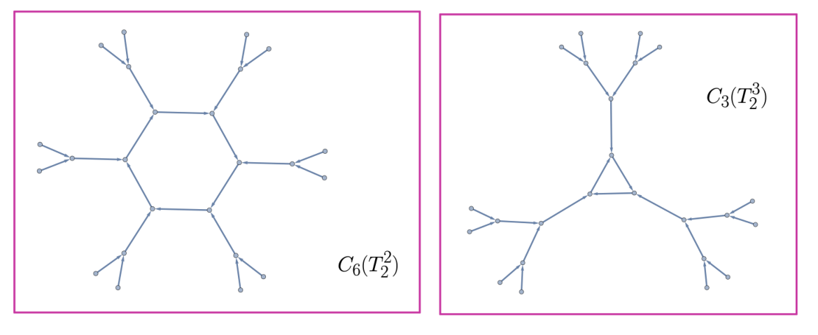
The graph appears often in the sequel (esp. with ), and we give a colloquial description here: start with a cycle of length , and then to each vertex in the cycle, “glue” a tree of type . In this picture, the nodes in the cycle itself are the periodic points, and the trees coming off each node are the preperiodic points that map into that particular orbit. See Figure 1 for a few examples.
Theorem 2.2.5.
[Structure of ] Let be an odd prime, and write . Write where is odd. (Note that is always even, so .) For each divisor of , take disjoint copies of , and is isomorphic to the disjoint union of these cycles over the divisors .
Remark 2.2.6.
Note that this implies that every vertex in has an in-degree of two or zero (note that the trees attached to the cycles are always of the form ).
To describe the result a bit more colloquially: we first compute , and pull out all possible powers of , until we obtain the odd number . From there, we enumerate all of the divisors of , and these determine all of the periodic orbits of . Then the number of powers of that we pulled out gives us the full structure of the pre-periodic points attached to these periodic orbits.
Onto the proof: we start with the following result that was proven by Gauss in [4]:
Proposition 2.2.7.
If , where is an odd prime, then is a cyclic group of order .
The fact that this group is cyclic allows us to more or less completely characterize the graph structure of . We follow the approach of [1] who completely characterized for prime in the same way (in this section the novelty is that we are extending these ideas to , but since is cyclic the same idea goes through).
We first give a definition and a lemma:
Definition 2.2.8.
We define as the graph whose vertices are the set and edges given by .
Lemma 2.2.9.
Let be any cyclic group of order (where here we denote the group operation as multiplication). Call one of its generators . We can define a function on by
This function is conjugate to the map , and so has the same dynamical structure (periodic orbits, fixed points, etc.) and its graph is isomorphic to .
Proof.
Let us define the maps with , with , and with . Since generates , the map is invertible. We see that , so and are conjugate. In particular, note that iff and moreover that iff , so that there is a one-to-one correspondence between the fixed/periodic points of and . In particular this implies that the two functions have isomorphic graphs. ∎
Basically we just need to understand . Under addition, this is a cyclic group of order , with generator . We stress here that we are now moving to additive notation for simplicity, so here the identity is and the generator is ; when we convert this back to the multiplicative group we will have an identity of and a generator of . Some standard results from group theory [3, §2.3] tell us that:
- 1.
For any dividing , the set of all elements with (additive) order is given by
- 2.
The set has elements;
- 3.
Since , these sets exhaust .
Let us first consider the case with odd:
Proposition 2.2.10.
Let be odd, and consider the map on . Then this map has a unique fixed point at , and all other elements are periodic under this map. The map leaves each of the invariant, and decomposes into a disjoint union of periodic orbits, each with period . (Note that since , there will be exactly such disjoint orbits and note that divides by Fermat’s Little Theorem.)
Proof.
We can see by inspection that no point other than is fixed by the map. Now note that since , the map is invertible, and is thus effectively a permutation. Therefore all points are periodic under repeated application of this map.
To prove the second claim in the proposition, note that is the set of points in with additive order , i.e. iff and if , . This is invariant under the map since is odd: if then , etc.
Let with , and if then for . This means that we have
which is equivalent to saying that . Since , this is true iff .
The period of is the smallest for which , which is the smallest for which , and this is by definition. ∎
We are now able to understand the cyclic group for more general .
Proposition 2.2.11.
Let where is odd, and again consider the map . Then the graph consists of flower cycles, specifically: replace every cycle of length in with a copy of .
Proof.
We first consider the basin of attraction of , which consists of the multiples of . (Note that for some iff is a multiple of .) In fact, we can see that if with and odd, then reaches 0 in exactly iterations, each passing through higher orders of . For example, all of the odd multiples of will be in the top layer (there will be exactly of these); the odd multiples of will be in the next layer (exactly of these), and so on. Note that every vertex in this tree has in-degree 2 or 0: nothing maps to the odd numbers in the top layer, but each subsequent number has two preimages: given an such that , we also have So in general, we have a tree of type with at the root, the point the single point in layer , the points in layer two (each of which map to ), the points in layer three, etc. We will call this the “tree rooted at 0” below.
We now claim that for any periodic orbit that appears in , there is a corresponding flower orbit in . Consider any period orbit in with elements . By definition, and . Now let and note that gives a periodic orbit modulo : if is a multiple of , then is a multiple of . Now pick any of the . We know that there is at least one that maps to (since it is part of a periodic orbit). Therefore there is another, that maps to , and this corresponds to the vertex in the tree rooted at 0. If is odd, then the tree terminates, but if it is even, there are two numbers that map to , namely and . As we move up the branches of this tree, each layer removes one power of two, and each vertex has exactly two vertices mapping to it, until we reach the ’th layer. Therefore there will be a attached to — and the same argument applies to any of the elements in any of the periodic orbits, and we are done.
∎
Corollary 2.2.12.
If for some power of , then the graph is a tree with layers. The th layer consists of the odd numbers, the st layer is those numbers that are two times an odd, etc. In particular, the graph is a .
One direct corollary of this is that if is a Fermat prime, then the graph is a tree.
2.3 The graph of nilpotent elements when is an odd prime
Now we can attack the case of those elements that are not units when is an odd prime.
Definition 2.3.1.
We say that is nilpotent modulo if there exists some power such that .
It is easy to see that is nilponent modulo iff . Also note that if then for any , and in particular it is true for being some power of two, so we have:
Lemma 2.3.2.
is nilpotent modulo for some . In particular, this implies that is a (connected) tree.
Now that we have established that is a tree and we want to determine its structure. It can actually have an interesting and complex structure, especially when is large. Our main result is the following.
Definition 2.3.3.
Let be an odd prime. Fix , and for each we define the tree recursively:
- 1.
If is odd: then is just a single node with no edges;
- 2.
If is even and has no preimages modulo : then then is just a single node with no edges;
- 3.
If is even and has two preimages modulo : denote these preimages by and , then is a rooted tree with trees mapping into this root:
copies of and copies of .
(Note by Remark 2.2.6 that this exhausts all possible cases.)
Theorem 2.3.4.
The graph is a rooted tree with as the root and vertices. The in-neighborhood of 0 is constructed as follows: for any and for any with , attach a tree of type , where , to 0. For any (where and ), write as the (unique) decomposition with , and the in-neighborhood of is the tree , where .
Remark 2.3.5.
Theorem 2.3.4 basically follows from the following lemma:
Lemma 2.3.6.
Consider , let (where ) and consider the equation
| (1) |
Write as the element of that is congruent to modulo . If is odd, or if is even and is a leaf in , then (1) has no solutions. If there are two numbers such that , then (1) has solutions. Half of these ( of them) are solutions of the form where and the other half are solutions of the form where .
Proof.
Let us first consider the case where as a warm-up; the general case is similar but has more details.
.Let us write , , and assume that . This tells us that
Note that we have and — this is the range of prefactors we can put in front of each of those powers.
Let us write and . If we consider the last equation modulo , this implies . This implies that if has no preimages in then there is no solution. Let us assume that has two preimages in , and pick one of them, say . If we can show that there are exactly solutions to the system of congruences
then we have established the result of the theorem for . Let us define two sets:
We can see that and , and of course maps into under the squaring map. Thus each point in is hit an average of times, but we want to show that it is exactly times. Let us parameterize by , with . We claim that as we run through these , the values of each get hit exactly times. First note that if we replace with , then we get
so we only need consider . We claim that these give distinct values modulo , and since there are of them, they must cover the set — and then shifting the arguments by gives the same values, and this gives us copies. All we need to show now is that every element of gets hit once as runs from to . We compute:
so we nowneed to show that the map has only one root on . If we assume that , then by taking modulo , this gives , and thus . From this we have , thus the same for , thus for , etc. From this we get that only can solve this equation, and we are done.
General .The argument is similar: writing , , and that . This tells us that
Note that we now have and . Again assume that has preimages in and call one . We now show that there are solutions to the system
Here we parameterize with . We obtain the same repeating argument when adding a multiple of , and so we only need to consider . But this will repeat times, so again we only need to show that every target gets hit in the cycle. But then the rest of the argument follows.
∎
Proof of Theorem 2.3.4.
The lemma does most of the work for us here. Note that implicit in the lemma that for any , if we write , then the basin of attraction of depends only on . We can go through the cases: if is odd, then has no preimages modulo by the lemma, and so it is a leaf in — and similarly for even but having no preimages modulo .
Finally, for the neighborhood of 0: note that if , then . Thus any such point maps to 0 under squaring, and the preimage of each of these points is a tree of type . ∎
Again it is worth pointing out that Lemma 2.3.6 tells us that basically all that matters is the mod value of the prefactor. We can now define a non-recursive way to compute the trees defined in Definition 2.3.3. We now describe an algorithm that will compute this tree exactly. We will state but not prove the algorithm.
Definition 2.3.7.
For any prime, and , we define the unfurled preimage of of depth , , as a directed tree. The vertices of are all sequences of the form with such that and . The edges of are
Remark 2.3.8.
It is always true that forms a tree, since each edge moves from a sequence to a strictly smaller sequence and thus cannot have loops. (The construction above is sometimes referred to as the “universal cover of the graph rooted at ”.
Proposition 2.3.9.
is always a tree with degree . If is a transient point then is a regular -tree. If is prime, and with odd, and , then is a regular -tree. Otherwise, it is not a regular -tree.
Example 2.3.10.
Assume that , so that . Let us first compute . Note that has two preimages: and , so is a regular -tree. Now, if we want to go to depth , we see that has no preimage, but again has two, so the note terminates, but the node bifurcates. Again, going to depth , we again terminate at and bifurcate at . Depending on the depth to which we want to unfurl this tree, we can continue as long as we’d like. Also note that we are labeling each node by the last term in the sequence defining the node, and not the whole sequence itself (it is useful to think of just this last value, but of course the sequence is important in the definition to give unique descriptors for each node). See Figure 2.
Now, consider any periodic . We claim that will be isomorphic to . To see this, note that since is periodic, it has two preimages: one is the periodic with , and the other is the preperiodic with , so we get a regular -tree at depth 1. To go to depth , we have that is periodic so it again bifurcates into the periodic and perperiodic , whereas is a leaf in , so it does not.
Definition 2.3.11 (Layered trees and expansions).
We say that is a layered tree with layers if can be written as the disjoint union of and every edge in the graph goes from layer to layer . (This is basically the directed version of -partite.) Note that a vertex in a layer- tree is a leaf iff it is in layer .
Given an -layer tree , and the integer vector , we define expanded by , to be the following -layer tree:
- 1.
Let be a vertex in the -th layer. Then the vectors of the form
are all in the -th later of .
- 2.
We define the edges of by
Lemma 2.3.12.
Let , and let for , and . Write , where is odd. Define as in Definition 2.3.7 and expand this graph by . Then this graph is isomorphic to the basin of attraction of in .
2.4 The graph
We have dealt with all powers of odd primes above, but still need to deal with . This will be a bit different than what has gone before, both for the units and the nilpotents, but it will be similar enough that we can reuse some earlier ideas here. First, a preliminary result that we can prove pretty simply.
Proposition 2.4.1.
Let . Then has exactly two components — one corresponding to and the other to , and they are both trees. (Equivalently, the graph has exactly two fixed points: and , and no periodic points.)
Proof.
The proof of the claim for is similar to that for odd primes. The nilpotent elements modulo are exactly the even numbers, and when these are raised to a high enough power, they will be 0 modulo . Now we consider the units, which are the odd numbers. Let with . Then , and
Since the power has increased, from this we see that any odd number will be 1 modulo in at most steps, and we are done. ∎
From this we just need to characterize each of the two trees. We consider first. One complication here is that the units modulo do not form a cyclic group under multiplication, but we get something that is close enough to make it work:
Lemma 2.4.2.
[4] The powers of 3 modulo form a cyclic group of size under multiplication. If we write as the set
then the units modulo (basically the odd numbers) can be written as .
Using Lemma 2.4.2, we can characterize :
Proposition 2.4.3.
The graph of is a tree constructed in the following manner: Start with the tree , and for every node that is not a leaf, add two leaves directly mapping into it.
Proof.
Since forms a cyclic subgroup of the units of size , the graph of these numbers can be realized as , which by Corollary 2.2.12 is . Note that all of the other units are negatives of powers of , and under squaring the negative sign cancels. So, for example, if is such that , then we also have , so that now has in-degree four. Moreover, if there is any leaf in the , i.e. a number in that is not a square modulo , then there can be no number in that squares to it, since the negative of that number would be in . Therefore if a number is a leaf in the original tree, then it remains a leaf when we add in the terms as well. ∎
See Figure 3 for an example with . We can also describe the graph intuitively as follows: Start with the node at and add a loop; add three nodes: and , which will be leaves, and the node , which will itself be a tree; to , we add four inputs: the leaves and , and two trees: and , etc.
Now onto the nilpotent elements. This case is a bit more complex than the case where is odd. The main problem here is that there is no statement analogous to Lemma 2.3.6 — the main idea there is that the basin of attraction of any point of the form depends only on the value of , whenever is odd. This is clearly not true in the case where , since this would mean that the basin of attraction for all numbers of the form would be the same, but this cannot be true since some odd numbers have square roots modulo and some do not (q.v. the discussion of units above). In particular, when computing the basin of attraction of a point , we didn’t need to pay attention to the “ambient space” , but unfortunately this breaks when . So in theory one can compute this tree for any given , but we don’t expect such a nice result as seen in Theorem 2.3.4 or Lemma 2.3.12. We do have a partial result that we state without proof.
Proposition 2.4.4.
Consider , and let , where . Let us define by the equations
where are odd. Define . Define as in Definition 2.3.3, add on the extra nodes as we did in Proposition 2.4.3, and expand it as in Definition 2.3.11, where we expand the first layer by , the second layer by , etc. Then the basin of attraction of is isomorphic to this expanded graph.
3 Specific Computations
3.1 Computing the Kronecker products in practice
As we have seen above, the type of graph structures we see for primes, or powers of primes, come in certain forms — and the graphs for composite come from Kronecker products of these. We have two main results in this section: the first is that one can compute the Kronecker product “component by component”, and the second one is a list of the typical graph products will we see in practice.
Definition 3.1.1.
If are are two graphs with disjoint vertex sets, then we define the disjoint union of and , denote , as the graph with and .
Now, let us assume that there is a path from to in . If we ignore the ’s, this gives a path from to in , and if we ignore the ’s, this gives a path from to in . Therefore if and are in the same component of , then and must be in the same component in , and and must be in the same component in . This gives the following:
Proposition 3.1.2.
Let and be graphs, and let
be the decomposition of each graph into its connected components. Then we have
where the individual terms in the union are themselves disjoint. More specifically, if there is a path from to in , then there must be a path from to in and one from to in .
Basically this means that we can compute the Kronecker product “component by component” — more specifically, when computing the Kronecker product we can just look at each component individually and not worry about the impact from other components. This is good, because we can compartmentalize. However, one caveat, as we will see below: it is possible for the product of two connected graphs to not be connected, so that some of the terms in the expansion above might not themselves be a single components, but can be multiple components. However, we do see that the number of connected components of is bounded below by the product of the numbers of connected components of and , respectively. Ok, so what do these component-by-component products actually look like?
As we learned from Theorems 2.2.5 and 2.3.4, every component of is either a flower cycle, or a looped tree (recall Definition 2.2.3). This, with Proposition 3.1.2, tells us that the natural question is what happens when we take the Kronecker product of two graphs which are each of one of these two types. We categorize all of the cases we might expect to see later in the following Proposition.
Proposition 3.1.3.
We have the following results:
- 1.
(Two looped trees) If and are looped trees, then so is — specifically, this implies that is connected, has a single root vertex, that root vertex loops to itself, and all vertices flow toward that root.
- 2.
(Degrees) Assume that and are looped trees with the property that every vertex in either has in-degree or . Then every vertex in has in-degree or .
- 3.
(Specific grounded trees) For any widths and depth , we have
(If we take two regular grounded trees of the same depth, then we get a regular grounded tree of that depth, just wider.)
- 4.
(Another description of flower cycles)
- 5.
(One looped tree and one flower cycle)
- 6.
(Two flower cycles) Let and . Let and . Then is disjoint copies of the graph .
Note the last case where two connected graphs have a disconnected product!
Proof.
- 1.
Consider the vector in , where each corresponds to the root in that tree. Then note that by definition, and we have this loop. More generally, if we take any , then there is a finite path from to in and a finite path from to in , so there is a finite path (whose length is the maximum of the two aforementioned paths) from to .
- 2.
In fact we prove something a bit more general: if has an in-degree of and has an in-degree of , then has an in-degree of . To see this, note that if for and for , then for all . The claim follows directly.
- 3.
Let us consider the case where we have two trees and . See Lemma 3.1.4 below for a parameterization of each of these trees. Then, the root of is where is the root of each . Note that it has a loop to itself. Let us define the first layer of to be any pair with but not both zero. Note that all of these map to in one step, and there are exactly of these. Now we define the th layer of : given pair where is in level of and is in level of , define . Note that any such vertex will map down to layer . Moreover, if , then each of these vertices has exactly preimages, because we can append numbers to the end of and numbers to the end of . If , then these elements are all leaves, and we are done.
- 4.
This is actually a bit trickier than it looks, since these two descriptions are isomorphic but not equal. Recall the definition of : we define the vertices of this graph to be where and . The edges in are defined as follows:
However, in (actually but who’s counting) we have
Now let us define a map as , where is the level of the vertex (in this case, the number of edges it takes to get from to ). Now, let us assume that in . This is true iff in , which if true iff in and . Now we claim that this is equivalent to in . Breaking up by cases: if , then , which would imply , and if , then , and , which would imply .
- 5.
This follows from the previous result twice and associativity, since
- 6.
Let us first note that if we consider two bare cycles, we get a similar formula: Let and . Note that we can think of these cycles as the map on and respectively, and here will be the graph of the map on . It is easy enough to see that the element has order , and so every point is on a periodic cycle of length . Since there are total vertices, and , there are exactly distinct periodic cycles.
To get the full case: we have
and we have computed above that is copies of .
∎
Lemma 3.1.4.
We can parameterize as follows: let , be the set and let
(These correspond to the “layers” in the graph, so any vertex in is “in layer ”.) Let . Now define edges as follows: for all , add an edge , and for all with , add the edge
i.e. throw out the last component. Then this graph is isomorphic to .
3.2 The same unit graph can show up in many places
A natural question is how similar the graphs can be for different . However, note that if we have two primes with , then , so they do not have isomorphic sets of units. But it is possible that we can have two primes with , and thus . For example, we have that
so . We now work both cases out. Since , we have (so the flowers on the cycle are just one node sticking out) and the divisors are . Since , there is one orbit of period , and since , there is one orbit of period . This determines the graph of units completely. For , of course, we have that is just with a loop to itself, but is more complicated. The set of points that map to zero modulo are the two points and . If we recall the graph , we see that has a preimage of , and has no preimage. Therefore is a leaf in , whereas is a tree of the form , which will be a regular tree of width and depth (there are three trees of type and three of type , which are themselves single nodes by definition, so are leaves in ). See Figure 4.

3.3 Example where we really go to town on the Kronecker products
As we proved in Proposition 3.1.3, all of the components that show up in are themselves Kronecker products of graphs that show up in the factors of other graphs. So, let’s say, for example, we want to find an that contains a copy of the graph
One way to obtain this is to find primes that contain such graphs, and then multiply these together. We know that a for prime will contain a iff is divisible by exactly powers of . For , we can pick , and for we can pick . For we cannot pick , since it’s not prime, and we don’t want to pick any even multiple of , as we’ll get too many powers of . So we can pick , and finally we can pick . Of course, , , and are relatively small since they are Fermat primes, but we need to stretch a bit for .
Now we know that the basin of attraction of in is exactly , for . We have , and therefore the basin of attraction of in is exactly , shown in Figure 5. (In fact, to generate this picture we actually just directly computed the subgraph of containing directly.) It’s a pretty wild graph: it has a radius of due to the term, but the smaller terms give it some interesting heterogeneity (e.g. each intermediate node has leaves hanging off of it, etc.).
In fact, we can completely understand the graph of using the tools above. Note that since are all Fermat primes, their graphs consist of a tree containing nodes, plus a with a loop, so is the union . For , we note that , and , so has a single loop of period in the form of a , plus a going to , plus the single loop at . There are 24 possible products in the expansion
and notice that there is only one loop that can be chosen in any of these products, so each product remains connected and there are precisely 24 components. Moreover, exactly eight of these will have a loop of period , and sixteen will not, for example for loops we can get a by choosing , but we can also get by choosing , etc.
In general, we can extrapolate directly from this example that for any flower cycle of the form , where is a tree that can be formed by taking Kronecker products of any collection of ’s, then we can find a (square-free) that contains .
3.4 Triggering divisors
Definition 3.4.1.
Given a period , we say that is a triggering divisor for if
- •
;
- •
for any that is a proper divisor of .
Remark 3.4.2.
It follows directly from the definition that iff is a multiple of a triggering divisor of .
The name “triggering divisor” comes from the fact that the presence of such a divisor of will trigger a periodic orbit of period . (It might be that other divisors of also give periodic orbits of period , but this minimal one is the one that triggers the condition…)
Corollary 3.4.3.
The graph has a flower orbit of type iff is a multiple of times a triggering divisor of .
Proof.
This follows directly from Theorem 2.2.5 and the definition of triggering divisor. ∎
We present the triggering divisors for all periods up to in Table 1, and we have also put the first for which a period appears. Note that the triggering divisors are not “unique” in some cases for certain periods — we can obtain multiple numbers, neither of which divides the other. Also note, interestingly, that these numbers might not even be relatively prime. In the table, when there are multiple triggering divisors we have bolded the one that gives rise to the first prime to have that period; for example, for period 18, the smallest prime that is is actually 191, whereas the smallest prime that is is 109.
Also, one might ask whether a composite number gives rise to a particular periodic orbit before any prime does. In theory it is possible that one could observe a (composite) period first in a composite number. For example, to obtain a period-10 orbit, we can find a prime that gets it from a triggering divisor (in this case, 47) or we could find a number with a period-2 and a period-5 and multiply them. So, for example, also has a period-10 orbit, but . In practice we never found an example where a period first shows up in a composite number but there are a lot of integers that we didn’t check. The author is agnostic on the claim as to whether a particular period length can ever show up first at a composite .
There is a lot of heterogeneity in how large the triggering divisors are. One thing that follows directly from the definitions is that
Proposition 3.4.4.
If is a Mersenne prime ( is prime and is also prime) then period- has the single triggering divisor .
One can see this markedly at in Table 1, whereas for primes that are not Mersenne primes (e.g. there is a “pretty small” triggering divisor.)
The method to obtain the values in Table 1 was as follows. For any period , we list all divisors of the number . For any that divides , we compute the multiplicative order of modulo and retain those where . (Of course, since divides , then must divide , but it could be strictly smaller.) From this retained list of divisors, we remove those divisors that are multiples of others in the list. For example, let us consider period . We have , the divisors of which are . We have and and remove those. Of the remaining three, we can compute that they satisfy . But then notice that is a multiple of (and also for that matter) so we throw out , leaving and . And also note that these divisors are independent in the sense that they give different sets of primes. For example, if we consider , then , which is not divisible by , and conversely has which is not divisible by . Note that in each of these cases, so we see that has a single period-6 orbit of type (since ) but has two disjoint such orbits (since ). See Figure 6.
| Period | Trig div | First | Period | Trig div | First |
| 1 | 1 | 1 | 26 | 2731,24573 | 60083 |
| 2 | 3 | 7 | 27 | 262657 | 2626571 |
| 3 | 7 | 29 | 28 | 29,113,215,635 | 59 |
| 4 | 5 | 11 | 29 | 233,1103,2089 | 467 |
| 5 | 31 | 311 | 30 | 77,99,279,331,453,651,1661 | 199 |
| 6 | 9, 21 | 19 | 31 | 2147483647 | ?? |
| 7 | 127 | 509 | 32 | 65537 | 917519 |
| 8 | 17 | 103 | 33 | 161,623,599479 | 967 |
| 9 | 73 | 293 | 34 | 43691,393213 | 87383 |
| 10 | 11,93 | 23 | 35 | 71,3937,122921 | 569 |
| 11 | 23,89 | 47 | 36 | 37,95,109,135,247,351,365,949 | 149 |
| 12 | 13,35,45 | 53 | 37 | 223,616318177 | 2677 |
| 13 | 8191 | 376787 | 38 | 174763,1572861 | 699053 |
| 14 | 43,381 | 173 | 39 | 79,57337,121369 | 317 |
| 15 | 151,217 | 907 | 40 | 187,425,527,697,61681 | 1123 |
| 16 | 257 | 1543 | 41 | 13367,164511353 | 106937 |
| 17 | 131071 | 1572853 | 42 | 147,301,387,1011,1143,2667,5419,14491 | 883 |
| 18 | 19,27,219 | 109 | 43 | 431,9719,2099863 | 863 |
| 19 | 524287 | 8388593 | 44 | 115,397,445,2113,3415 | 461 |
| 20 | 25,41,55,155 | 83 | 45 | 631,2263,11023,23311 | 6311 |
| 21 | 49,337,889 | 197 | 46 | 141,535443,2796203 | 283 |
| 22 | 69,267,683 | 139 | 47 | 2351,4513,13264529 | 4703 |
| 23 | 47,178481 | 283 | 48 | 97,673,1799,2313,3341,61937 | 389 |
| 24 | 119,153,221,241 | 239 | 49 | 4432676798593 | ?? |
| 25 | 601,1801 | 3607 | 50 | 251,1803,4051,5403,6611,19811 | 503 |

3.5 When cycles beget many more cycles
Consider the two numbers considered in the previous section: the primes and . These numbers were chosen as primes that give period-6 orbits, but “for different reasons”, because they derive from independent triggering divisors. Since they both have periodic orbits of the same period, if we take the Kronecker product, we will obtain many orbits of that period, from Proposition 3.1.3, since — so that the product of two period-6 cycles is actually 6 distinct period-6 cycles.
Again, we first consider . Since , we need to consider the divisors of . We already saw that we have an orbit of period , and from the divisor we get and orbit of period . Since we have attached to the graphs (just giving a “spoke”). Therefore has four components, namely
For , we have , and so we need to consider the divisors . As we computed above, the gives two period-6 orbits. Since and , the term gives two period-3 orbits, and gives one period two orbit. Therefore has 7 components:
Now let us consider . We know that the graph will contain at least components, since one of the graphs has 4 and the other 7. But in fact, it will have many more components: each time we take the product of two period-6 orbits, we actually get six period-6 orbits, etc.
For example, let us consider the component of , and multiply it against the seven components of . We get
And also note that the first two components listed above each appear twice in , so when we multiply by the components of we obtain copies of and one copy of .
When we multiply the component of against the other seven, we obtain
This gives a total of copies of , one copy of , and one copy of .
The other two components are simpler, since they are trees. Multiplying against the components of gives copies of , copies of , copy of , copy of , and finally one copy of . Multiplying against these components just copies them.
Putting this all together, we have
| Graph type | copies |
|---|---|
| 21 + 6 +2 = 29 | |
| 2 | |
| 1+1=2 | |
| 1 + 1 +1 = 3 | |
| 1 + 1 + 1 = 3 | |
| 1 + 1 + 1 = 3 | |
| 1 | |
| 1+1=2 | |
| 1 |
We can compare this against the graph given in Figure 7, which was obtained by direct computation. Note that will be a cycle of period with three leaves sticking out of each node, and will be a cycle of period with a single stem out of each node.
3.6 When the nilpotents end up chillin’ in the corner
Consider . Here we want to study the graph , and in particular, focus on .
Let us use the formula in Theorem 2.3.4. We first compute the graph . Recalling the graph , we see that has two preimages: and , and has two preimages: and . In this case the actual values of the preimages won’t be important, since is a leaf regardless of , due to the single power of .
According to the theorem, has five incoming copies of and five incoming copies of , but these are all leaves, so is just a regular tree of width , or . We get the same result for . And, of course, is just a single node.
We also have that is a node simply because is odd.
Now, the in-neighborhood of will be any numbers with 2 or 3 powers of in them. There are four such preimages with power three ( for , which are all nodes) and such preimages of power two. As we say above, half of these are trees and the other half are nodes. Putting all of this together, the in-neighborhood of is copies of and leaves. See Figure 8, where we have plotted .
Note the structure is as we say: the node has fourteen leaves leading into it: the four that come from terms: 125, 250, 375, 500, and the ten that come from terms, where the prefactor is or modulo 5: . We also see that there are ten trees that go into , coming from terms, where the prefactor is or modulo 5: .
Of course, if we want to understand the full graph we also need to consider the units. Note that . The divisors are , where we have , so one period-100 orbit, , so one period-20 orbit, , so one period-4 orbit, and of course one fixed point. Since these are all decorated with copies of , so in fact we have
so has five components, see Figure 9. (We can see that the tree is just chilling down there in the corner.)
3.7 Well, *these* nilpotents ain’t messing around
Here we are going to describe the graph when .
First we consider . We have , so we have and . The divisors of are, of course, for . In each of these cases, it turns out that , so we have exactly 11 periodic orbits: a fixed point, one of period 2, one of period 6, etc. all the way up to one of period . Since , all of these periodic orbits have a “spoke” coming out of each periodic point.
Now for . Let us first consider the neighborhood of : any of the form with will map directly into 0. If is odd, then these are leaves. If is even but , then this is also a leaf. In the other cases, we will have some more complex trees. For each even , if is we have a tree of type , giving a total of of them, and if is it is a leaf, so we have leaves. If is odd we have leaves. Therefore the total number of leaves is .
From here we see that we should have attached to :
| Tree type | leaves | |||
| Count | 1 | 9 | 81 | 151 |
Moreover, we can see that since , is just a tree of depth one, since iff with and , and there are such ’s, so is just a regular tree of width and depth . Similarly, is a tree of depth 1 and width .
The more complicated case is . Note that , so we can consider the unfurled graph of depth three , see Figure 2. According to Lemma 2.3.12, we take this graph and expand it by the powers , so that the in-neighborhood of has leaves coming in, and trees of type , which themselves have leaves coming in, and trees coming in, and those are regular trees of the form . (And of course, for any with we get an isomorphic tree, so there are of them.) See Figure 10 for a visualization of , which is also complicated and fun. (We would have liked to put a visualization of the full here but at vertices and edges, it made our computer sad.)

4 Conclusions
We have presented some basic theory and give a few nice examples. The examples were a lot of fun, and there’s no doubt that one can find a whole host of other interesting examples. I leave it to the readers of this article to explore and find more.
References
- [1] Troy Vasiga and Jeffrey Shallit. On the iteration of certain quadratic maps over GF(p). Discrete Mathematics, 277(1-3):219–240, 2004.
- [2] Lee DeVille. What does look like??? YouTube video, May 17, 2022. https://www.youtube.com/watch?v=RmqFm9HN3nw
- [3] David Dummit and Richard Foote. Abstract Algebra, volume 1999. Prentice Hall Englewood Cliffs, NJ, 1991.
- [4] Carl Friedrich Gauss. Disquisitiones Arithmeticae. English edition. translated by Arthur A. Clarke, 1986.