A micropolar shell model for hard-magnetic soft materialsJournal: JOURNAL

Magneto-active soft materials consist of magnetic particles dispersed into a soft elastomeric matrix and undergo large deformations under magnetic loading. This class of materials has been used in vibration absorbers, sensors, actuators, soft robots, flexible electronics, and isolators (see, e.g., Ren2019, Wu2020, Bastola2021, Bastola2020, Lucarini2022, Yarali2022 and references therein). Therefore, developing reliable theoretical models plays an essential role in the optimum and cost-effective design of the aforementioned devices and instruments.

Based on the type of the embedded particles, magneto-active soft materials are divided into two sub-classes, namely soft-magnetic soft materials (SMSMs) and hard-magnetic soft materials (HMSMs). The former contains particles with low coercivity, such as iron or iron oxides, and their magnetization vector varies under external magnetic loading. This sub-class has been the subject of a huge amount of research work in this century (e.g., Saxena2013, Miehe2016, Mehnert2017, Mukherjee2020, Bustamante2021, Hu2022, akbari2020). The latter sub-class is composed of particles of high coercivity, such as CoFe₂O₄ or NdFeB, so that their magnetization vector, or equivalently, their remnant magnetic flux, remains unchanged for a wide range of the applied external magnetic flux (e.g., Schumann2020, Lee2020). One of the main characteristics of HMSMs is that external magnetic induction of relatively small magnitude causes rapid finite deformations in these materials (e.g., Lum2016, Wu2019). Moreover, the 3D printing technologies have enabled the researchers to program the ferromagnetic domains in complex structures, which leads to the desired deformations Kim2018, Alapan2020, Kuang2021, Wang2021, Wu2021.

Theoretical modeling of HMSMs has been the subject of a plethora of research articles in recent years (e.g., Kalina2017, Zhao2019, Garcia2019, Mukherjee2021, rambausek2022, Zhang2020, Garcia2021a, Garcia2021b, Ye2021, DH2022IJSS). In particular, Zhao et al. Zhao2019 developed a continuum formulation with asymmetric Cauchy stress so that the external magnetic induction directly contributes to the expression of the stress tensor. Their theory has been the foundation for the analysis of hard-magnetic soft beams (HMSBs) in Yan et al. Yan2021, Wang et al. Wang2020, Rajan and Arockiarajan Rajan2021, and Chen et al. Chen2020a, Chen2021 among others. The same formulation has been employed to model the deformation of magneto-active shells by Yan et al. Reis2021. Dadgar-Rad and Hossain DH2022EML enhanced the formulation of Zhao et al. Zhao2019 to account for viscoelastic effects and analyzed the time-dependent dissipative response of HMSBs. Some researchers have developed micromechanical and lattice models for HMSMs (e.g., Refs. Zhang2020, Garcia2021a, Garcia2021b, Ye2021). From a different point of view, Dadgar-Rad and Hossain DH2022IJSS focused on the well-known phenomenon that due to the presence of the remnant magnetic induction in HMSMs, applying an external magnetic loading produces a body couple that plays the role of the main driving load to generate mechanical deformation in the body (e.g., Dorfmann2014). Moreover, the Cauchy stress losses its symmetry, as had been previously pointed out by Zhao et al. Zhao2019. However, instead of following the methodology advocated in Zhao2019, the authors developed a formulation based on micropolar continuum theory to predict the deformation of 3D hard-magnetic soft bodies. Two significant differences between the results of the formulation of Zhao et al. Zhao2019 and those based on the micropolar-enhanced formulation have been expressed by Dadgar-Rad and Hossain DH2022IJSS.

Eringen and his coworkers established the theoretical foundations of micropolar theory Kafadar1971, Eringen1976, Eringen1999. In this theory, a microstructure at each material point is considered. The microstructure can have arbitrary rigid rotations independent of the traditional motion field considered in the classical continuum. Formulations of the micropolar theory to model localized elastic-plastic deformations (e.g., Borst1993, Steinmann1994, Tsakmakis2005, Grammenoudis2007a, Grammenoudis2007b, Bauer2012a, Borst2022) and size-dependent elastic deformations (e.g., Pietraszkiewicz2009, Ramezani2008, Ramezani2009, Bauer2010, Bauer2012b, Erdelj2020) have been developed. Some formulations to model micropolar shells have been also proposed (e.g., Sargsyan2020, Eremeyev2005, Eremeyev2017). Moreover, the theory has been used in the modeling of lattice structures, crystal plasticity, phononic crystals, chiral auxetic lattices, phase-field fracture mechanics, and vertebral trabecular bone Yoder2018, Mayeur2011, Zapata2020, Spadoni2012, Goda2014, Suh2020.

The current research is essentially the continuation of the previous work of the authors, namely Dadgar-Rad and Hossain DH2022IJSS, which had been developed for three-dimensional bodies. However, most bodies made of HMSMs are thin structures, and using three-dimensional elements is computationally expensive. Accordingly, the purpose of this research is to develop a micropolar-based shell model to predict the deformation of thin HMSMs. To do so, the 7-parameter shell formulation of Sansour (e.g., Sansour98, SansKoll2000) has been extended to a 10-parameter one that involves the micro-rotation of the microstructure. On the other hand, the enhanced assumed strain method (EAS) is a widely-used strategy to eliminate locking in shell structures, e.g., SimoArmero92, Simo93, KW96, Glaser97. Therefore, this method is adopted here to circumvent locking effects in the present micropolar shell formulation.

The next sections of this paper are as follows: The basic kinematic and kinetic relations of the micropolar continuum theory are summarized in Section 2. In Section 3, the main characteristics of HMSMs are presented. In Section 4, the kinematic equations describing a 10-parameter micropolar shell model are provided. Section 5 presents the variational formulation, followed by a FE formulation in Section 6. Numerical examples are studied in Section 7, and the paper concludes in Section 8.

Notation: In this work, Greek indices take $1$ and $2$. All upper-case and lower-case Latin indices take $1$, $2$, and $3$. Upper-case indices with calligraphic font, e.g., $\mathcal{K}$ and $\mathcal{L}$, take the values specified in the corresponding equations. The repeated Latin and Greek indices obey Einstein’s summation convention. If $\mathbb{P}$ and $\mathbb{Q}$ are two 2nd-order tensors, the tensorial products defined via the symbols $\otimes$, $\odot$, and $\boxtimes$ generate 4th-order tensors so that the corresponding components are given by $(\boldsymbol{\mathcal{C}})_{ijkl}=(\mathbb{P}\otimes\mathbb{Q})_{ijkl}=P_{ij}Q_{kl}$, $(\boldsymbol{\mathcal{B}})_{ijkl}=(\mathbb{P}\odot\mathbb{Q})_{ijkl}=P_{ik}Q_{jl}$, and $(\boldsymbol{\mathcal{C}})_{ijkl}=(\mathbb{P}\boxtimes\mathbb{Q})_{ijkl}=P_{il}Q_{kj}$, respectively. For numerical simulations, the notation $\mathbbm{U}=\{U_{11},U_{22},U_{33},U_{12},U_{21},U_{13},U_{31},U_{23},U_{32}\}^{\scriptscriptstyle\mskip-1.0mu\top\mskip-2.0mu}$ will be used as the $9\times 1$ vectorial representation of the arbitrary 2nd-order tensor $\mathbb{U}$.

The purpose of this section is to introduce some concepts and relations of the micropolar theory. The interested reader may refer to the pioneering works developed in Refs. Eringen1976, Eringen1999, Steinmann1994 for more details and discussions.

In this section, two coincident Cartesian coordinates $\{X_{I}\}$ and $\{x_{i}\}$, with $\{\mathbbm{E}_{I}\}$ and $\{\mathbbm{e}_{i}\}$ as the corresponding basis vectors, are considered. The center of a macro-element in the reference configuration $\mathcal{B}_{0}$ is denoted by $\mathbbm{X}$. After deformation by the deformation mapping $\boldsymbol{\psi}$, the center of the macro-element in the current configuration $\mathcal{B}$ at the time $t$ is denoted by $\mathbbm{x}$, so that $\mathbbm{x}=\boldsymbol{\psi}(\mathbbm{X},t)$. The deformation gradient $\mathbb{F}$ is given by

which can be uniquely decomposed as $\mathbb{F}=\mathbb{R}\mathbb{U}=\mathbb{V}\mathbb{R}$. Here, $\mathbb{R}$ is the macro-rotation tensor, and $\mathbb{U}$ and $\mathbb{V}$ are the symmetric positive definite right and the left stretch tensors, respectively. For later use, the variation of the deformation gradient is written as follows:

Moreover, $\hat{\mathbbm{u}}=\mathbbm{x}-\mathbbm{X}$ and $\delta\hat{\mathbbm{u}}=\delta\mathbbm{x}$ are the actual and virtual displacement fields, respectively.

As a basic assumption in the micropolar theory, there exists a microstructure inside each macro-element so that it experiences rigid micro-rotations independent of the macro-motion $\mathbbm{x}$. Let $\boldsymbol{\theta}=\theta_{i}\mathbbm{e}_{i}$ denote the micro-rotation pseudo-vector, and $\theta=(\theta_{i}\theta_{i})^{1/2}$ be its magnitude. The corresponding micro-rotation tensor, denoted by $\tilde{\mathbb{R}}$, can be expressed via the Euler–Rodriguez formula, namely (e.g., Steinmann1994, Ramezani2009)

where $\hat{\boldsymbol{\theta}}=-\boldsymbol{\mathcal{E}}\boldsymbol{\theta}$, or $\hat{\theta}_{ij}=-\epsilon_{ijk}\theta_{k}$, is the skew-symmetric tensor corresponding to $\boldsymbol{\theta}$. Moreover, $\epsilon_{ijk}$ are the components of the alternating symbol $\boldsymbol{\mathcal{E}}$. By defining $\delta\boldsymbol{\theta}$ as the virtual micro-rotation pseudo-vector, the variation of $\tilde{\mathbb{R}}$ may be expressed via the following relations Ramezani2009, DH2022IJSS

The deformation gradient, in the micropolar theory, is decomposed as $\mathbb{F}=\tilde{\mathbb{R}}\tilde{\mathbb{U}}=\tilde{\mathbb{V}}\tilde{\mathbb{R}}$, from which it follows that (e.g., Steinmann1994):

To take the gradient of the micro-rotation into account, the material wryness tensor $\boldsymbol{\Gamma}$ and its spacial counterpart $\boldsymbol{\gamma}$, are defined by Eringen1976, Eringen1999, Steinmann1994, Pietraszkiewicz2009

The deformation measures $\tilde{\mathbb{U}}$ and $\boldsymbol{\Gamma}$ are the main kinematic tensors to develop a formulation in material framework (see also, Refs. Eringen1976, Steinmann1994). Combinations of Eqs. (2), (4), (5)₁, and (6)₁, furnishes the following relations for the virtual kinematic tensors $\delta\tilde{\mathbb{U}}$ and $\delta\boldsymbol{\Gamma}$ DH2022IJSS:

where $\delta\hat{{\boldsymbol{\omega}}}=-\boldsymbol{\mathcal{E}}\delta{\boldsymbol{\omega}}$ is the skew-symmetric tensor corresponding to $\delta{{\boldsymbol{\omega}}}$.

Next, in the current configuration $\mathcal{B}$, let $\text{d}\mathcal{A}$ and $\mathbbm{n}$ be an infinitesimal area element and its corresponding outward unit normal vector, respectively. In the micropolar theory, the traction $\mathbbm{t}^{(\mathbbm{n})}$ and the couple vector $\mathbbm{s}^{(\mathbbm{n})}$ (as the moment per unit area) act on $\text{d}\mathcal{A}$. Let $\boldsymbol{\sigma}$ and $\mathbb{m}$ be the asymmetric Cauchy stress and the asymmetric couple stress corresponding to $\mathbbm{t}^{(\mathbbm{n})}$ and $\mathbbm{s}^{(\mathbbm{n})}$, respectively. Accordingly, the well-known Cauchy’s stress principle is extended as follows (e.g., DH2022IJSS, Eringen1976):

For later use, the first Piola–Kirchoff stress $\mathbb{P}$, the material stress $\tilde{\mathbb{P}}$, the first Piola–Kirchoff couple stress $\mathbb{M}$, and the material couple stress $\tilde{\mathbb{M}}$ are defined by

The main property of hard-magnetic soft materials is the existence of a remnant magnetic flux density, that remains almost unchanged under a wide range of the applied external magnetic flux $\mathbbm{B}^{\text{ext}}$ (e.g., Lum2016, Wu2019, Zhao2019). Let $\tilde{\mathbbm{B}}^{\text{rem}}$ and ${\mathbbm{B}}^{\text{rem}}$ be the remnant magnetic flux in the reference and current configurations, respectively. The relation between $\tilde{\mathbbm{B}}^{\text{rem}}$ and ${\mathbbm{B}}^{\text{rem}}$ is as follows Zhao2019:

The action of $\mathbbm{B}^{\text{ext}}$ on ${\mathbbm{B}}^{\text{rem}}$ leads to a body couple (moment per unit volume) in HMSMs. The relations for the body couple per unit current volume $\mathbbm{p}$, and the body couple per unit reference volume $\mathbbm{p}^{\ast}$ may be written as (e.g., Zhao2019, Dorfmann2014)

where the constant $\mu_{0}=4\pi\times 10^{-7}\frac{N}{A^{2}}$ is the free space magnetic permeability. For HMSMs, the external magnetic flux density $\mathbbm{B}^{\text{ext}}$ is often assumed to remain constant in space (e.g., Refs. Zhao2019, Wang2020, Chen2020a, Chen2021, Rajan2021). Using this point, it has been proven that the following Maxwell equations are satisfied in HMSMs (e.g., Zhao2019, Dorfmann2014):

where $\mathbbm{B}$ is the referential magnetic flux density, $\mathbbm{H}$ is the referential magnetic field, $\mathbbm{E}_{I}$ is the basis vector of the referential coordinate system $\{X_{I}\}$ defined in the previous section, and "Curl" is the referential curl operator.

The geometry of a part $\mathcal{P}$ of a shell in the reference and current configurations is displayed in Fig. 1. Let $\mathcal{S}_{0}$ be the mid-surface of the shell in the reference configuration, which deforms into the surface $\mathcal{S}$ in the current one. As shown in Fig. 1, in addition to the two common-frame Cartesian coordinates $\{X_{I}\}$ and $\{x_{i}\}$, described in the previous section, the convective coordinate system $\{\zeta^{i}\}$ at each material particle $q$ of the reference mid-surface $\mathcal{S}_{0}$ is also constructed. The coordinate lines $\zeta^{i}$ deform during the motion of the shell in space so that the coordinated lines $\zeta^{1}$ and $\zeta^{2}$ are tangent to both $\mathcal{S}_{0}$ and $\mathcal{S}$. Moreover, the coordinated line $\zeta^{3}\in[-{\textstyle{\frac{1}{2}}}h,{\textstyle{\frac{1}{2}}}h]$, with $h$ as the initial thickness of the shell, is considered to be perpendicular to $\mathcal{S}_{0}$ in the reference configuration. However, it does not remain perpendicular to $\mathcal{S}$ in the current configuration, in general. In the sequel, for the sake of simplicity, the coordinate $\zeta^{3}$ may be replaced by $z$.

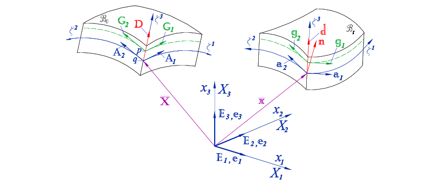
The position of the material particle $q$ on the mid-surface $\mathcal{S}_{0}$ may be described by the vector $\mkern 1.5mu\overline{\mkern-1.5mu\mathbbm{X}\mkern-1.5mu}\mkern 1.5mu(\zeta^{1},\zeta^{2})$. Let $\{\mathbbm{A}_{\alpha},\mathbbm{A}^{\alpha},A_{\alpha\beta},A^{\alpha\beta},\mathbbm{D},\mathbb{B}\}$ be, respectively, the covariant and contravariant basis vectors, covariant and contravariant components of the metric tensor, outward unit normal vector, and the curvature tensor on the undeformed mid-surface $\mathcal{S}_{0}$. Then the following relations from the differential geometry of surfaces hold (e.g., I19):

where $\delta_{\alpha}^{\beta}$ is the two-dimensional Kronecker delta. For later use, the surface contravariant basis vectors may be written as $\mathbbm{A}^{\alpha}=A^{\ast\alpha J}\mathbbm{E}_{J}$, where $A^{\ast\alpha J}$ are the Cartesian components of $\mathbbm{A}^{\alpha}$. The position of the material particle $p$ located at the elevation $z$ with respect to $\mathcal{S}_{0}$ is described by

from which the covariant basis vectors $\mathbbm{G}_{i}$ are obtained to be

Motivated by Eqs. (13)₈ and (15), the symmetric shifter tensor $\mathbb{Q}=\mathbb{Q}^{\scriptscriptstyle\mskip-1.0mu\top\mskip-2.0mu}=\mathbbm{G}_{i}\otimes\mathbbm{A}^{i}=\mathbb{I}-z\mathbb{B}$, with ${\mathbb{I}}$ as the identity tensor, is defined. The shifter tensor can be used to map the covariant and contravariant basis vectors from $z\neq 0$ to the mid-surface with $z=0$, and vice versa. More precisely, the following relations hold:

where $\mathbbm{G}^{i}$ are the contravariant basis vectors at $\mathbbm{X}$, and use has been made of the symmetry property of $\mathbb{Q}$. For later use, the three-dimensional material gradient operator $\text{Grad}_{\boldsymbol{\zeta}}$, with respect to the convective coordinates $\{\zeta^{i}\}$ in the reference configuration, and the material surface gradient operator $\text{Grad}_{\mathcal{S}_{0}}$ with respect to $\{\zeta^{\alpha}\}$ are defined as follows:

By assuming that a straight material fiber perpendicular to $\mathcal{S}_{0}$ remains straight during deformation, the following macro deformation field is considered (e.g., Sansour98, SansKoll2000):

where $\mkern 1.5mu\overline{\mkern-1.5mu\mathbbm{x}\mkern-1.5mu}\mkern 1.5mu$ is the image of $\mkern 1.5mu\overline{\mkern-1.5mu\mathbbm{X}\mkern-1.5mu}\mkern 1.5mu$ on $\mathcal{S}$, and $\mathbbm{d}$ is a director vector along the deformed $z$-axis. Moreover, the scalar field $\phi$ describes through the thickness stretching of the shell. Similar to the quantities defined on $\mathcal{S}_{0}$ in Eq. (13), let $\{\mathbbm{a}_{\alpha},\mathbbm{a}^{\alpha},a_{\alpha\beta},a^{\alpha\beta},\mathbbm{n},\mathbb{b}\}$ be the surface quantities defined on $\mathcal{S}$. It then follows that

Moreover, based on Eq. (18), the covariant basis vectors $\mathbbm{g}_{i}$ at $\mathbbm{x}$ are as follows:

It is observed from Eq. (20)₂ that the director $\mathbbm{d}$ and the basis vector $\mathbbm{g}_{3}$ are in the same direction. However, the normal vector $\mathbbm{n}$ and $\mathbbm{g}_{3}$ are not in the same direction, in general. Next, the vectors $\mathbbm{u}=u_{i}\mathbbm{e}_{i}$ and $\mathbbm{w}=w_{i}\mathbbm{e}_{i}$ are defined as the mid-surface and the director displacements, respectively. This allows one to write

From Eqs. (16) and (17)₁, the deformation gradient tensor $\mathbb{F}$, described in the convective coordinate system $\{\zeta^{i}\}$, takes the form

In the present shell model, using Eqs. (15), (16)₃, (20), and (22), and neglecting the higher-order terms involving $z^{2}$, the deformation gradient is approximated as follows:

and the tensors $\mathbb{F}^{[0]}$ and $\mathbb{F}^{[1]}$, with the aid of Eqs. (13)₈ and (21), are given by

To circumvent numerical difficulties in finite element solution, the in-plane deformation gradient term $\mathbb{F}^{[0]}$ is enhanced by the second-order tensor $\bar{\mathbb{F}}$, to be introduced in Section 6. Accordingly, the term $\mathbb{F}^{[0]}$ in Eq. (23)₂ is replaced by $\mathbb{F}^{[0]}+\bar{\mathbb{F}}$. Moreover, following Ramezani and Naghadabadi RamezBeam in the context of the micropolar Timoshenko beam model, it is assumed that the micro-rotation pseudo-vector is constant along the shell thickness, namely $\boldsymbol{\theta}=\tilde{\boldsymbol{\theta}}(\zeta^{1},\zeta^{2})$. Accordingly, the micro-rotation tensor $\tilde{\mathbb{R}}(\boldsymbol{\theta})$ is independent of the $z$ coordinate. Keeping this in mind and using Eqs. (5)₁, (6)₁, (16)₃, (17)₂, and (23), the micropolar deformation measures $\tilde{\mathbb{U}}$ and $\boldsymbol{\Gamma}$, in the present shell formulation, may be written as

where $\mathbb{F}^{\ast}=\tilde{\mathbb{F}}+\bar{\mathbb{F}}$ is the enhanced form of $\tilde{\mathbb{F}}$. The present formulation with $\{\mathbbm{u},\mathbbm{w},\phi,\boldsymbol{\theta}\}$ as the unknown field variables may be regarded as a 10-parameter micropolar shell model. In other words, the present formulation is the extension of the classical 7-parameter shell model, with $\{\mathbbm{u},\mathbbm{w},\phi\}$ as its unknowns, introduced by Sansour (e.g., Sansour98, SansKoll2000).

Let $\delta\mathcal{U}$ be the virtual internal energy and $\delta\mathcal{W}$ denote the virtual work of external loads. The principle of virtual work states that $\delta\mathcal{U}-\delta\mathcal{W}=0$ Wriggers2008. In what follows, the expressions for $\delta\Psi$ and $\delta\hat{\mathcal{W}}$, as, respectively, $\delta\mathcal{U}$ and $\delta\mathcal{W}$ per unit reference volume, are derived. Moreover, for the linearization purpose to be used in the next section, the increments of $\delta\Psi$ and $\delta\hat{\mathcal{W}}$ are also calculated.

By neglecting thermal effects, assuming that the material is hyperelastic, and to develop a material formulation, the internal energy per unit reference volume may be written as $\Psi=\tilde{\Psi}(\tilde{\mathbb{U}},\boldsymbol{\Gamma})$ Eringen1976, Steinmann1994. Using this point and Eq. (7) furnishes

Moreover, the constitutive equations for the pairs $\{\tilde{\mathbb{P}},\tilde{\mathbb{M}}\}$ and $\{\mathbb{P},\mathbb{M}\}$ are as follows DH2022IJSS:

It is noted that Eqs. (26) and (27) hold for all three-dimensional micropolar hyperelastic solids. For the present shell model, first the quantities denoted by $\delta\boldsymbol{\Upsilon}^{[\mathcal{J}]}$ ($\mathcal{J}=1,2$) are defined by

Next, after replacing $\tilde{\mathbb{F}}$ by the enhanced form $\mathbb{F}^{\ast}$, combination of Eqs. (25), (26)₁, (27)_1,2, and (28) leads to the following expression for $\delta\Psi$:

For linearization purpose, the increment of $\delta\Psi$ under the increment of the field variables $\Delta\mathbbm{u}$, $\Delta\mathbbm{w}$, $\Delta\phi$, and $\Delta\boldsymbol{\theta}$ is needed. Accordingly, from Eqs. (26)₁, (27), and (29) it is deduced that

where $\Delta\delta\mathbb{H}^{[1]}$ and $\Delta\delta\mathbb{H}^{[2]}$ are as follows:

Moreover, the fourth-order tensors $\boldsymbol{\mathcal{C}}^{[\mathcal{I}]}$ ($\mathcal{I}=1,2,3,4$) have the following components:

and $\tilde{\mathcal{C}}^{[\mathcal{I}]}_{PJQL}$ are the components of the following fourth-order tensors:

In this work, the micropolar-enhanced neo-Hookean constitutive model proposed in Ref. DH2022IJSS is employed, according to which the free energy density is given by

where $\eta$ is a material constant, and $l$ is the well-known material length-scale parameter. From Eqs. (27)₁ and (34), the expressions for $\tilde{\mathbb{P}}$ and $\tilde{\mathbb{M}}$ are then calculated to be DH2022IJSS

Moreover, Eqs. (33) and (34) lead to the following 4th-order tensors $\tilde{\boldsymbol{\mathcal{C}}}^{[\mathcal{I}]}$:

Next, it is recalled that $\mathbbm{B}^{\text{ext}}$ induces the body couple density $\mathbbm{p}^{\ast}$ on an HMSM (c.f. Eq. (11)₂). Since $\mathbbm{p}^{\ast}$ and $\boldsymbol{\theta}$ are work-conjugate quantities, the virtual external work density $\delta\hat{\mathcal{W}}$ and its increment may be written as

As will be shown in the next section, Eq. (37)₂ leads to the expression for the load stiffness matrix. The expressions for $\delta\Psi$, $\Delta\delta\Psi$, $\delta\hat{\mathcal{W}}$, and $\Delta\delta\hat{\mathcal{W}}$ given in Eqs. (29), (30), and (37) are the basic relations for the FE formulation presented in the next section.

A nonlinear finite element formulation for the present shell model is developed in this section. Let $\mathcal{S}_{0}^{\mathfrak{e}}$ be a typical element in the referential mid-surface $\mathcal{S}_{0}^{\mathfrak{e}}$. To perform numerical integration, the typical element is mapped to the two-dimensional parent square element $\square=[-1,1]\times[-1,1]$ in the $\{\xi,\eta\}$ space, with $\xi,\eta\in[-1,1]$. The field variables $\{u_{i},w_{i},\theta_{i},\phi\}$, over the parent element $\mathcal{S}_{0}^{\mathfrak{e}}$, are interpolated as follows:

where $\mathbbm{N}_{u}=\{N_{u}^{1},N_{u}^{2},...,N_{u}^{n_{u}}\}$ is a row vector containing the shape functions that interpolate the mid-surface displacement $u_{i}$ over the element. Here, $n_{u}$ is the number of nodes of the element that possess the $u_{i}$-DOF. Let $U_{i}^{\mathcal{I}}$ be the displacement component $u_{i}$ at the $\mathcal{I}$’th node ($\mathcal{I}=1,2,...,n_{u}$) of the element. Accordingly, $\mathbbm{U}_{i}=\{U_{i}^{1},U_{i}^{2},...,U_{i}^{n_{u}}\}^{\scriptscriptstyle\mskip-1.0mu\top\mskip-2.0mu}$ is a column vector that involves all $U_{i}^{\mathcal{I}}$’s over the element. Similar definitions hold for the other quantities in Eq. (38). Moreover, similar relations hold for the increment $\{\Delta u_{i},\Delta w_{i},\Delta\theta_{i},\Delta\phi\}$ and variation $\{\delta u_{i},\delta w_{i},\delta\theta_{i},\delta\phi\}$ of the field variables. The generalized displacement vector ${\mathbbm{v}}^{\mathfrak{e}}$ involving all nodal DOFs of the typical element may be written as

where $n^{\mathfrak{e}}=3(n^{u}+n^{w}+n^{\theta})+n^{\phi}$ is the number of nodal DOFs. Based on Esq. (2), (24), (28), and (38), the following relations hold:

Here, the last equality in each relation indicates that all components can be expressed in terms of the generalized virtual displacement vector $\delta{\mathbbm{v}}^{\mathfrak{e}}$. Next, the enhanced deformation gradient tensor $\bar{\mathbb{F}}$ is considered. Let $\boldsymbol{\alpha}=\{\alpha_{1},\alpha_{2},...,\alpha_{\mathcal{P}^{\ast}}\}^{\scriptscriptstyle\mskip-1.0mu\top\mskip-2.0mu}$ be the column vector of enhanced parameters $\alpha_{\mathcal{P}}$’s ($\mathcal{P}=1,2,...,\mathcal{P}^{\ast}$), where $\mathcal{P}^{\ast}$ is the total number of enhanced parameters. The components of $\bar{\mathbb{F}}$ and its variation/increment depend linearly on $\alpha_{\mathcal{P}}$’s (see, e.g., Refs. SimoArmero92, Simo93, KW96, Glaser97). Here, following the notation used in Eq. (40), one may write

where $\bar{\mathbbm{b}}_{iJ}$ are the $\mathcal{P}^{\ast}\times 1$ row vectors, $\bar{\mathbbm{F}}$ is the $9\times 1$ vectorial representation of $\bar{\mathbb{F}}$, and $\bar{\mathbbm{B}}$ is a $9\times\mathcal{P}^{\ast}$ matrix the rows of which are $\bar{\mathbbm{b}}_{iJ}$.

Now, let $\mathbbm{B}^{(\mathcal{N})}$ ($\mathcal{N}=0,1,2$) and $\mathbbm{B}^{[\omega F]}$ be the $9\times n^{\mathfrak{e}}$ matrices whose rows are $\mathbbm{b}^{(\mathcal{N})}_{iJ}$ and $\mathbbm{b}^{[\omega F]}_{iJ}$, respectively. From Eqs. (28), (40), and (41) it then follows that

The differential volume element $\text{d}\mathcal{V}^{\mathfrak{e}}_{0}$ located at the elevation $z$ with respect to the typical element $\mathcal{S}^{\mathfrak{e}}_{0}$ is given by (e.g., Sansour98)

Now, the element virtual internal energy is given by $\delta\mathcal{U}^{\mathfrak{e}}=\int_{\mathcal{V}_{0}^{\mathfrak{e}}}\Psi\text{d}\mathcal{V}_{0}^{\mathfrak{e}}$. Similarly, the expression for the virtual work over the element can be calculated via $\delta\mathcal{W}^{\mathfrak{e}}=\int_{\mathcal{V}_{0}^{\mathfrak{e}}}\hat{\mathcal{W}}\text{d}\mathcal{V}_{0}^{\mathfrak{e}}$. Using Eqs. (28) and (42), the expressions for $\delta\mathcal{U}^{\mathfrak{e}}$ and $\delta\mathcal{W}^{\mathfrak{e}}$ may be written as

where the internal force vectors $\mathbbm{F}^{\text{int}v}$ and $\mathbbm{F}^{\text{int}\alpha}$ are as follows:

Moreover, the external force vector $\mathbbm{F}^{\theta}_{\text{ext}i}$, work conjugate to $\boldsymbol{\Theta}_{i}$, is given by

Next, the linearized equations resulting from Eqs. (30), (37)₂, and (44) may be written as

The system of algebraic equations extracted from Eq. (47) may be written as

where the subscripts "mat", "geo", and "load", represent the material, geometric, and load part of the element stiffness matrix. In particular, the material sub-matrices $\mathbbm{K}^{vv}_{\text{mat}}$, $\mathbbm{K}^{v\alpha}_{\text{mat}}$, and $\mathbbm{K}^{\alpha\alpha}_{\text{mat}}$ in Eq. (48) are as follows:

where $\mathbbm{C}^{[\mathcal{J}]}$ are the matrix forms of $\boldsymbol{\mathcal{C}}^{[\mathcal{J}]}$. Moreover, the load sub-matrices $\mathbbm{K}^{vv}_{\text{load}}$, $\mathbbm{K}^{v\alpha}_{\text{load}}$ are given by

References

- [1] Ren Z, Hu W, Dong X, Sitti M. Multi-functional soft-bodied jellyfish-like swimming. Nature Commun. 2019;10:2703.
- [2] Wu S, Hu W, Ze Q, Sitti M, Zhao R. Multifunctional magnetic soft composites: a review. Multifuct Mater. 2020;3:042003.
- [3] Bastola AK, Paudel M, Li L, Li W. Recent progress of magnetorheological elastomers: a review. Smart Mater Struct. 2020;29:123002.
- [4] Bastola AK, Hossain M. The shape-morphing performance of magnetoactive soft materials. Mat Des. 2021;211:110172.
- [5] Lucarini S, Hossain M, Garcia-Gonzalez D. Recent advances in hard-magnetic soft composites: synthesis, characterisation, computational modelling, and applications. Compos Struct. 2022;200:210001.
- [6] Yarali E, Banishadi M, Zolfagharian A, Chavoshi M, Arefi F, Hossain M, Bastola B, Ansari M, Foyouzat A, Dabbagh A, Ebrahimi M, Mirzaali MJ, Bodaghi M. Magneto/electroresponsive polymers toward manufacturing, characterization, and biomedical/soft robotic applications. Appl Mater Today. 2022;26:101306.
- [7] Saxena P, Hossain M, Steinmann P. A theory of finite deformation magneto-viscoelasticity. Int J Solids Struct. 2013;50:3886–3897.
- [8] Ethiraj G, Miehe C. Multiplicative magneto-elasticity of magnetosensitive polymers incorporating micromechanically-based network kernels. Int J Eng Sci. 2016;102;93–119.
- [9] Mehnert M, Hossain M, Steinmann P. Towards a thermo-magneto-mechanical coupling framework for magneto-rheological elastomers. Int J Solids Struct. 2017;128:117–132.
- [10] Mukherjee D, Bodelot L, Danas K. Microstructurally-guided explicit continuum models for isotropic magnetorheological elastomers with iron particles. Int J Non-Linear Mech. 2020;120:103380.
- [11] Bustamante R, Shariff MHBM, Hossain M. Mathematical formulations for elastic magneto-electrically coupled soft materials at finite strains: Time-independent processes. Int J Eng Sci. 2021;159:103429.
- [12] Hu X, Zhu H, Chen S, Yu H, Qu S. Magnetomechanical behavior of soft magnetoactive membranes. Int J Solids Struct. 2022;234–235:111310.
- [13] Akbari E, Khajehsaeid H. A continuum magneto-mechanical model for magnetorheological elastomers. Smart Mater Struct. 2020;30:015008.
- [14] Schümann M, Borin DY, Morich J, Odenbach S. Reversible and non-reversible motion of NdFeB-particles in magnetorheological elastomers. J Intell Mater Syst Struct. 2020;32:3–15.
- [15] Lee M, Park T, Kim C, Park SM, Characterization of a magneto-active membrane actuator comprising hard magnetic particles with varying crosslinking degrees. Mater Des. 2020;195:108921.
- [16] Lum GZ, Ye Z, Dong X, Marvi H, Erin O, Hu W, Sitti M. Shape-programmable magnetic soft matter. Proc Natl Acad Sci. 2016;113:6007–6015.
- [17] Wu S, Ze Q, Zhang R, Hu N, Cheng Y, Yang F, Zhao R. Symmetry-breaking actuation mechanism for soft robotics and active metamaterials. ACS Appl Mater Interfaces. 2019;11:41649–41658.
- [18] Kim Y, Yuk H, Zhao R, Chester SA, Zhao X. Printing ferromagnetic domains for untethered fast-transforming soft materials. Nature, 2018;558:274–279.
- [19] Alapan Y, Karacakol AC, Guzelhan SN, Isik I, Sitti M. Reprogrammable shapemorphing of magnetic soft machines. Sci Adv. 2020;6:eabc6414.
- [20] Kuang X, Wu S, Ze Q, Yue L, Jin Y, Montgomery SM, Yang F, Qi HJ, Zhao R. Magnetic dynamic polymers for modular assembling and reconfigurable morphing architectures. Adv Mater. 2021;2102113.
- [21] Wang L, Zheng D, Harker P, Patel AB, Guo CF, Zhao X. Evolutionary design of magnetic soft continuum robots. Proc Natl Acad Sci. 2021;118:21.
- [22] Wu S, Hamel CM, Ze Q, Yang F, Qi HJ, Zhao R. Evolutionary algorithm-guided voxel-encoding printing of functional hard-magnetic soft active materials. Adv Intell Syst. 2021;2:2000060.
- [23] Kalina KA, Brummund J, Metsch P, Kaestner M, Borin DY, Linke JM, Odenbach S. Modeling of magnetic hystereses in soft MREs filled with NdFeB particles. Smart Mater Struct. 2017;26:105019.
- [24] Zhao R, Kim Y, Chester AS, Sharma P, Zhao X. Mechanics of hard-magnetic soft materials. J Mech Phys Solids. 2019;124:244–263.
- [25] Garcia-Gonzalez D. Magneto-visco-hyperelasticity for hard-magnetic soft materials: theory and numerical applications. Smart Mater Struct. 2019;28:085020.
- [26] Mukherjee D, Rambausek M, Danas K. An explicit dissipative model for isotropic hard magnetorheological elastomers. J Mech Phys Solids. 2021;151:104361.
- [27] Rambausek M, Mukherjee D, Danas K. A computational framework for magnetically hard and soft viscoelastic magnetorheological elastomers. Comput Methods Appl Mech Eng. 2021;391:114500.
- [28] Zhang R, Wu S, Qiji Z, Zhao Z. Micromechanics study on actuation efficiency of hard-magnetic soft active materials. J Appl Mech. 2020;87:091008.
- [29] Garcia-Gonzalez D, Hossain M. A microstructural-based approach to model magneto-viscoelastic materials at finite strains. Int J Solids Struct. 2021;208–209:119–132.
- [30] Garcia-Gonzalez D, Hossain M. Microstructural modelling of hard-magnetic soft materials: Dipole–dipole interactions versus Zeeman effect. Extreme Mech Lett. 2021;48:101382.
- [31] Ye H, Li Y, Zhang T. Magttice: A lattice model for hard-magnetic soft materials. Soft Matter. 2021;17:3560–3568.
- [32] Dadgar-Rad F, Hossain M. Finite deformation analysis of hard-magnetic soft materials based on micropolar continuum theory. Int J Solids Struct. 2022;251:111747.
- [33] Yan D, Abbasi A, Reis PM. A comprehensive framework for hard-magnetic beams: reduced-order theory, 3D simulations, and experiments. Int J Solids Struct. 2021; https://doi.org/10.1016/j.ijsolstr.2021.111319.
- [34] Wang L, Kim Y, Guo GF, Zhao X. Hard-magnetic elastica. J Mech Phys Solids. 2020;142:104045.
- [35] Rajan A, Arockiarajan A. Bending of hard-magnetic soft beams: A finite elasticity approach with anticlastic bending. Eur J Mech A/Sol. 2021;90:104374.
- [36] Chen W, Yan Z, Wang L. Complex transformations of hard-magnetic soft beams by designing residual magnetic flux density. Soft Matter, 2020;16:6379–6388.
- [37] Chen W, Wang L, Yan Z, Luo B. Three-dimensional large-deformation model of hard-magnetic soft beams. Compos Struct. 2021;266:113822.
- [38] Yan D, Pezzulla M, Cruveiller L, Abbasi A, Reis PM. Magneto-active elastic shells with tunable buckling strength. Nature Commun. 2021;12:2831.
- [39] Dadgar-Rad F, Hossain M. Large viscoelastic deformation of hard-magnetic soft beams. Extreme Mech Lett. 2022;54:101773.
- [40] Dorfmann A, Ogden RW. Nonlinear Theory of Electroelastic and Magnetoelastic Interactions. Springer; 2014.
- [41] Kafadar CB, Eringen AC. Micropolar media–I the classical theory. Int J Eng Sci. 1971;9:271–307.
- [42] Eringen AC, Kafadar CB. Polar field theories. In: Eringen AC (Ed.), Continuum Physics, vol. IV. Academic Press; 1976; 1–73.
- [43] Eringen AC. Microcontinuum Field Theories, vol. I, Foundations and Solids. Springer; 1999.
- [44] de Borst R. A generalization of -flow theory for polar continua. Comput Methods Appl Mech Eng. 1993;103:347–362.
- [45] Steinmann P. A micropolar theory of finite deformation and finite rotation multiplicative elastoplasticity. Int J Solids Struct. 1994;31:1063–1084.
- [46] Grammenoudis P, Tsakmakis C. Finite element implementation of large deformation micropolar plasticity exhibiting isotropic and kinematic hardening effects. Int J Numer Meth Eng. 2005;62:1691–1720.
- [47] Grammenoudis P, Tsakmakis C. Micropolar plasticity theories and their classical limits. Part I: Resulting model. Acta Mech. 2007;189:151–175.
- [48] Grammenoudis P, Sator C, Tsakmakis C. Micropolar plasticity theories and their classical limits. Part II: Comparison of responses predicted by the limiting and a standard classical model. Acta Mech. 2007;189:177–191.
- [49] Bauer S, Dettmer WG, Peric D, Schäfer M. Micropolar hyper-elastoplasticity: constitutive model, consistent linearization, and simulation of 3D scale effects. Int J Numer Meth Eng. 2012;91:39–66.
- [50] de Borst R, Alizede Sabet S, Hageman T. Non-associated Cosserat plasticity. Int J Mech Sci. 2022; https://doi.org/10.1016/j.ijmecsci.2022.107535.
- [51] Ramezani S, Naghdabadi R, Sohrabpour S. Non-linear finite element implementation of micropolar hypo-elastic materials. Comput Methods Appl Mech Eng. 2008;197:4149–4159.
- [52] Ramezani S, Naghdabadi R, Sohrabpour S. Constitutive equations for micropolar hyper-elastic materials. Int J Solids Struct. 2009;46:2765–2773.
- [53] Pietraszkiewicz W, Eremeyev VA. On natural strain measures of the non-linear micropolar continuum. Int J Solids Struct. 2009;46:774–787.
- [54] Bauer S, Schäfer M, Grammenoudis P, Tsakmakis C. Three-dimensional finite elements for large deformation micropolar elasticity. Comput Methods Appl Mech Eng. 2010;199:2643–2654.
- [55] Bauer S, Dettmer WG, Peric D, Schäfer M. Micropolar hyper-elasticity: constitutive model, consistent linearization and simulation of 3D scale effects. Comput Mech. 2012;50:383–396.
- [56] Erdelj SG, Jelenić G, Ibrahimbegović A. Geometrically non-linear 3D finite-element analysis of micropolar continuum. Int J Solids Struct. 2020;202:745–764.
- [57] Eremeyev VA. Nonlinear micropolar shells: Theory and applications. In: Pietraszkiewicz W, Szymczak C. (Eds.), Shell structures: Theory and Applications. Taylor & Francis; 2005; 11–18.
- [58] V.A. Eremeyev, H. Altenbach, Basics of mechanics of micropolar shells. In: Altenbach H, Eremeyev VA. (Eds.), Shell-like Structures. Springer; 2017; 63–111.
- [59] Sargsyan A, Sargsyan S. Geometrically nonlinear models of static deformation of micropolar elastic thin plates and shallow shells. Z Angew Math Mech. 2020;e202000148.
- [60] Yoder M, Thompson L, Summers J. Size effects in lattice structures and a comparison to micropolar elasticity. Int J Solids Struct. 2018;143:245–261.
- [61] Mayeur JR, McDowell DL, Bammann DJ. Dislocation-based micropolar single crystal plasticity: Comparison of multi- and single criterion theorie. J Mech Phys Solids. 2011;59:398–422.
- [62] Guarín-Zapata N, Gomez J, Valencia C, Dargush GF, Hadjesfandiari AR. Finite element modeling of micropolar-based phononic crystals. Wave Motion 2020;92:102406.
- [63] Spadoni A, Ruzzene M. Elasto-static micropolar behavior of a chiral auxetic lattice. J Mech Phys Solids. 2012;60:156–171.
- [64] Goda I, Assidi M, Ganghoffer GF. A 3D elastic micropolar model of vertebral trabecular bone from lattice homogenization of the bone microstructure. Biomech Model Mechanobiol. 2014;13:53–83.
- [65] Suh SS, Sun W-C, O’Connor DT. A phase field model for cohesive fracture in micropolar continua. Comput Methods Appl Mech Eng. 2020;369:113181.
- [66] Sansour C. Large strain deformations of elastic shells, constitutive modelling and finite element analysis. Comput Methods Appl Mech Eng. 1998;161:1–18.
- [67] Sansour C, Kollmann FG. Families of 4-node and 9-node finite elements for a finite deformation shell theory, an assessment of hybrid stress, hybrid strain and enhanced strain elements. Comput Mech. 2000;24:435–447.
- [68] Simo JC, Armero F. Geometrically non-linear enhanced strain mixed methods and the method of incompatible modes. Int J Numer Methods Eng. 1992;33:1413–1449.
- [69] Simo JC, Armero F, Taylor RL. Improved versions of assumed enhanced strain tri-linear elements for 3D finite deformation problems. Comput Methods Appl Mech Eng. 1993;110:359–386.
- [70] Korelc J, Wriggers P. Consistent gradient formulation for a stable enhanced strain method for large deformations, Eng Comput. 1996;13:103–123.
- [71] Glaser S, Armero F. On the formulation of enhanced strain finite elements in finite deformations. Eng Comput. 1997;14:759–791.
- [72] Itskov M. Tensor Algebra and Tensor Analysis for Engineers. Springer; 2019.
- [73] Ramezani S, Naghdabadi R, Sohrabpour S. Analysis of micropolar elastic beams. Eur J Mech A/Sol. 2009;28:202–208.
- [74] Wriggers P. Nonlinear Finite Element Methods. Springer; 2008.
- [75] Argyris J. An excursion into large rotations. Comput Methods Appl Mech Eng. 1982;32:85–155.
- [76] Yan B, Li B, Kunecke F, Gu Z, Guo L. Polypyrrole-based implantable electroactive pump for controlled drug microinjection. ACS Appl Mater Interfaces. 2018;7:14563–14568.
- [77] Ju Y, Hu R, Xie Y, Yao J, Li X, Lv Y, Han X, Cao Q, Li L. Reconfigurable magnetic soft robots with multimodal locomotion. Nano Energy. 2021;87:106169.
- [78] Carpenter JA, Eberle TB, Schuerle S, Rafsanjani A, Studart AR. Facile manufacturing route for magneto-responsive soft actuators. Adv Intell Syst. 2021;3:20000283.
- [79] Kadapa C, Hossain M. A unified numerical approach for soft to hard magneto-viscoelastically coupled polymers. Mech Mat. 2022;166:104207.