跳到论文正文
W Papers独立论文阅读器 arXiv:2207.10239 论文正文 计算阅读时间 · 0%
引用这篇论文根据当前论文元数据生成,正式投稿前建议核对。


License: CC BY 4.0
arXiv:2207.10239v3 [math.ST] 21 Feb 2023

Fixed-domain Posterior Contraction Rates for Spatial Gaussian Process Model with Nugget

Cheng Li Thanks: stalic@nus.edu.sg Affiliation: Department of Statistics and Data Science, National University of Singapore    Saifei Sun Thanks: sunsf1015@163.com Affiliation: Department of Statistics and Data Science, National University of Singapore    Yichen Zhu Thanks: yichen.zhu@duke.edu Affiliation: Department of Statistical Science, Duke University
Abstract

Spatial Gaussian process regression models typically contain finite dimensional covariance parameters that need to be estimated from the data. We study the Bayesian estimation of covariance parameters including the nugget parameter in a general class of stationary covariance functions under fixed-domain asymptotics, which is theoretically challenging due to the increasingly strong dependence among spatial observations. We propose a novel adaptation of the Schwartz’s consistency theorem for showing posterior contraction rates of the covariance parameters including the nugget. We derive a new polynomial evidence lower bound, and propose consistent higher-order quadratic variation estimators that satisfy concentration inequalities with exponentially small tails. Our Bayesian fixed-domain asymptotics theory leads to explicit posterior contraction rates for the microergodic and nugget parameters in the isotropic Matérn covariance function under a general stratified sampling design. We verify our theory and the Bayesian predictive performance in simulation studies and an application to sea surface temperature data.

Keywords: Bayesian inference, Matérn covariance function, Evidence lower bound, Higher-order quadratic variation.

1 Introduction

Gaussian process has been widely used in spatial statistics for modeling spatial and spatiotemporal correlations. This paper studies the parameter estimation in the following spatial Gaussian process regression model:

Y⁡(𝐬)=f​(𝐬)T​β+X⁡(𝐬)+ε⁡(𝐬), for ​𝐬∈[0,1]d,\displaystyle Y(\mathbf{s})=\mathrm{f}(\mathbf{s})^{\mathrm{\scriptscriptstyle T}}\beta+X(\mathbf{s})+\varepsilon(\mathbf{s}),\text{ for }\mathbf{s}\in[0,1]^{d}, (1)

where dd is the dimension of domain, f⁡(⋅)=(f1​(⋅),…,fp​(⋅))T∈ℝp\mathrm{f}(\cdot)=(\mathrm{f}_{1}(\cdot),\ldots,\mathrm{f}_{p}(\cdot))^{\mathrm{\scriptscriptstyle T}}\in\mathbb{R}^{p} is a pp-dimensional vector of deterministic known functions on [0,1]d[0,1]^{d}, and β∈ℝp\beta\in\mathbb{R}^{p} is the regression coefficient vector. In applications, f1,…,fp\mathrm{f}_{1},\ldots,\mathrm{f}_{p} can include the constant function 11, and hence β\beta can include an intercept term. The term X⁡(⋅)X(\cdot) is a Gaussian process X={X⁡(𝐬):𝐬∈[0,1]d}X=\left\{X(\mathbf{s}):\mathbf{s}\in[0,1]^{d}\right\}, and {ε⁡(𝐬):𝐬∈[0,1]d}\{\varepsilon(\mathbf{s}):\mathbf{s}\in[0,1]^{d}\} is a Gaussian white noise process independent of X⁡(⋅)X(\cdot) that satisfies ε⁡(𝐬)∼𝒩⁡(0,τ)\varepsilon(\mathbf{s})\sim\Ncal(0,\tau) for all 𝐬∈[0,1]d\mathbf{s}\in[0,1]^{d}. In practice, we observe the process Y⁡(⋅)Y(\cdot) and the functions f⁡(⋅)\mathrm{f}(\cdot) on a set of distinct sampling points Sn={𝐬1,…,𝐬n}⊆[0,1]dS_{n}=\{\mathbf{s}_{1},\ldots,\mathbf{s}_{n}\}\subseteq[0,1]^{d}. The observed data from the model (1) are Yn=(Y⁡(𝐬1),…,Y⁡(𝐬n))TY_{n}=(Y(\mathbf{s}_{1}),\ldots,Y(\mathbf{s}_{n}))^{\mathrm{\scriptscriptstyle T}} and Fn=(f​(𝐬1)T,…,f​(𝐬n)T)∈ℝn×pF_{n}=(\mathrm{f}(\mathbf{s}_{1})^{\mathrm{\scriptscriptstyle T}},\ldots,\mathrm{f}(\mathbf{s}_{n})^{\mathrm{\scriptscriptstyle T}})\in\mathbb{R}^{n\times p}. All statistical inference is based on the data (Yn,Fn)(Y_{n},F_{n}).

Model (1) is one of the most important models in spatial statistics and can be used as building blocks for other more sophisticated models. Besides the regression term f​(𝐬)T​β\mathrm{f}(\mathbf{s})^{\mathrm{\scriptscriptstyle T}}\beta, the Gaussian process term X⁡(⋅)X(\cdot) captures the spatial association and explains the spatial random effects from unmeasured or unobserved covariates with spatial pattern (Banerjee et al. 2008). The noise ε⁡(⋅)\varepsilon(\cdot) captures the measurement error, whose variance parameter τ\tau is also known as the nugget parameter.

It remains to specify the Gaussian process for X⁡(⋅)X(\cdot). We assume that the mean function of X⁡(⋅)X(\cdot) is zero, and the covariance function of X⁡(⋅)X(\cdot) can be written as Cov(X⁡(𝐬),X⁡(𝐭))=θ​Kα,ν​(𝐬−𝐭)\Cov(X(\mathbf{s}),X(\mathbf{t}))=\theta K_{\alpha,\nu}(\mathbf{s}-\mathbf{t}) for 𝐬,𝐭∈[0,1]d\mathbf{s},\mathbf{t}\in[0,1]^{d}, where θ>0\theta>0 is the microergodic parameter that will be defined later, Kα,ν​(⋅):ℝd→ℝK_{\alpha,\nu}(\cdot):\mathbb{R}^{d}\to\mathbb{R} is a positive definite function, α\alpha is the spatial range parameter, and ν\nu is the smoothness parameter. We will give several examples of covariance functions with this form in Section 2. For example, one popular choice in spatial statistics is the Matérn covariance function (Stein 1999)

Cov(X⁡(𝐬),X⁡(𝐭))=σ2​21−νΓ⁡(ν)​(α​‖𝐬−𝐭‖)ν​𝒦ν⁡(α​‖𝐬−𝐭‖),\displaystyle\Cov(X(\mathbf{s}),X(\mathbf{t}))=\sigma^{2}\frac{2^{1-\nu}}{\Gamma(\nu)}\left(\alpha\|\mathbf{s}-\mathbf{t}\|\right)^{\nu}\Kcal_{\nu}\left(\alpha\|\mathbf{s}-\mathbf{t}\|\right), (2)

where ν>0\nu>0 is the smoothness parameter, σ2>0\sigma^{2}>0 is the variance (partial sill) parameter, α>0\alpha>0 is the inverse range (or length-scale) parameter, Γ⁡(⋅)\Gamma(\cdot) is the gamma function, 𝒦ν⁡(⋅)\Kcal_{\nu}(\cdot) is the modified Bessel function of the second kind, and ∥⋅∥\|\cdot\| is the Euclidean norm. If we let θ=σ2​α2​ν\theta=\sigma^{2}\alpha^{2\nu} and K⁡(x)={21−ν/Γ⁡(ν)}​(‖x‖/α)ν​𝒦ν⁡(α​‖x‖)K(x)=\{2^{1-\nu}/\Gamma(\nu)\}\left(\|x\|/\alpha\right)^{\nu}\Kcal_{\nu}\left(\alpha\|x\|\right) for x∈ℝdx\in\mathbb{R}^{d}, then (2) can be written as θ​Kα,ν​(𝐬−𝐭)\theta K_{\alpha,\nu}(\mathbf{s}-\mathbf{t}) for 𝐬,𝐭∈[0,1]d\mathbf{s},\mathbf{t}\in[0,1]^{d}. For the Gaussian processes XX and YY in Model (1), we write X∼𝒢(0,θ​Kα,ν)X\sim\gp(0,\theta K_{\alpha,\nu}) and Y∼𝒢(βT​f,θ​Kα,ν+τ​δ0)Y\sim\gp(\beta^{\mathrm{\scriptscriptstyle T}}\mathrm{f},\theta K_{\alpha,\nu}+\tau\delta_{0}), respectively, where δ0\delta_{0} denotes the Dirac delta function at zero.

We study the Bayesian inference of Model (1) (Handcock and Stein 1993, De Oliveira et al. 1997), where the common practice is to assign prior distributions on the regression coefficients β\beta, the nugget parameter τ\tau, and the parameters in the covariance function of X⁡(⋅)X(\cdot) such as θ\theta and α\alpha. Bayesian posterior inference, including the prediction of Y⁡(s∗)Y(s^{*}) at a new location s∗∈[0,1]ds^{*}\in[0,1]^{d}, is fully based on the posterior distribution of these model parameters. In application, these parameters are randomly drawn from their posterior using sampling algorithms such as Markov chain Monte Carlo. Therefore, the behavior of their posterior distributions will heavily affect the Bayesian posterior predictive performance. However, despite the routine practice of using them in spatial statistics, there is a severe lack of theoretical understanding of Bayesian parameter estimation in the general spatial Gaussian process regression model with nugget (1), especially on the asymptotic behavior of the posterior distribution of model parameters when the number of observations becomes large. Such theory becomes increasingly important given the advance in high-resolution remote sensing technology, and the research on Gaussian process with massive spatial datasets is prevalent in Bayesian spatial statistics, such as Banerjee et al. 2008, Sang and Huang 2012, Datta et al. 2016, Heaton et al. 2019, Katzfuss and Guinness 2021, Peruzzi et al. 2022, Guhaniyogi et al. 2022, etc.

We consider the Bayesian fixed-domain asymptotics (or infill asymptotics) framework (Stein 1999, Zhang 2004). For the first time in the literature, we derive the fixed-domain Bayesian posterior contraction rates of model parameters in the general spatial Gaussian process regression model (1) with both the regression term f​(𝐬)T​β\mathrm{f}(\mathbf{s})^{\mathrm{\scriptscriptstyle T}}\beta and the measurement error (with the nugget τ\tau). In the fixed-domain asymptotics regime, the spatial domain [0,1]d[0,1]^{d}, as we have assumed, always remains fixed and bounded. This implies that as nn increases, the sampling locations in SnS_{n} become increasingly dense in the domain [0,1]d[0,1]^{d}, leading to increasingly stronger dependence between adjacent observations in the data YnY_{n}. The fixed-domain asymptotics has several advantages over other regimes such as increasing-domain asymptotics (Mardia and Marshall 1984). First, a fixed domain matches up with the reality in many spatial applications. For instance, the advances in remote sensing technology enable routine collection of spatial data in larger volume and higher resolution from a given region (Sun et al. 2018). Second, the stationarity assumption on the Gaussian process X⁡(⋅)X(\cdot) is more likely to hold on a fixed domain rather than an expanding domain. Therefore, the fixed-domain asymptotics regime is more suitable for interpolation of spatial processes (Section 3.3 of Stein 1999). Third, fixed-domain asymptotics has better parameter estimation performance than the increasing-domain asymptotics (Zhang and Zimmerman 2005).

On the other hand, fixed-domain asymptotics also poses several significant theoretical challenges. We take the isotropic Matérn covariance function for example. The first challenge comes from the lack of identification for the covariance parameters (σ2,α)(\sigma^{2},\alpha) in (2) when the domain dimension d=1,2,3d=1,2,3, due to the increasingly stronger dependence in the data YnY_{n}. We briefly review some basic results in equivalence of Gaussian processes. If two Gaussian processes are defined on a fixed domain, then by the result in Ibragimov and Rozanov 1978 and Chapter 4 of Stein 1999, they must be either equivalent or orthogonal to each other, where the equivalence means that their Gaussian measures are mutually absolutely continuous. In particular, Zhang 2004 has shown the well-known result that when the spatial domain has the dimension d=1,2,3d=1,2,3, for two isotropic Matérn with parameters (σ12,α1)(\sigma^{2}_{1},\alpha_{1}) and (σ22,α2)(\sigma^{2}_{2},\alpha_{2}) and the same smoothness ν\nu, their Gaussian measures are equivalent if σ12​α12​ν=σ22​α22​ν\sigma_{1}^{2}\alpha_{1}^{2\nu}=\sigma_{2}^{2}\alpha_{2}^{2\nu}, and they are orthogonal otherwise. This equivalence result for d=1,2,3d=1,2,3 is a consequence of the integral test for the spectral densities of two covariance functions; see for example, Theorem A.1 of Stein 2004. On the other hand, when d≥5d\geq 5, Anderes 2010 has proposed consistent moment estimators for both σ2\sigma^{2} and α\alpha with a given ν\nu under fixed-domain asymptotics. Recently Bolin and Kirchner 2023 have shown that for any d≥4d\geq 4, two Gaussian measures are equivalent if and only if they have the same parameters (σ2,α,ν)(\sigma^{2},\alpha,\nu), though finding the consistent estimators of (σ2,α)(\sigma^{2},\alpha) for d=4d=4 under fixed-domain asymptotics requires further study.

A direct consequence of the theory on equivalence of Gaussian processes is that for the domain dimension d=1,2,3d=1,2,3, which is of primary interest to spatial statistics, only the microergodic parameter θ=σ2​α2​ν\theta=\sigma^{2}\alpha^{2\nu} and continuous functions of θ\theta can be consistently estimated from the data under fixed-domain asymptotics. However, the individual variance parameter σ2\sigma^{2} and range parameter α\alpha have no consistent estimators when d=1,2,3d=1,2,3, and therefore they cannot have Bayesian posterior consistency. In general, the microergodic parameter is defined to be the parameter that uniquely determines the equivalence class of Gaussian processes; see Section 6.2 of Stein 1999 for a detailed explanation on the microergodic parameter. Besides Matérn, the exact form of microergodic parameter θ\theta for d=1,2,3d=1,2,3 has been identified in several other families, such as generalized Wendland (Bevilacqua et al. 2019) and confluent hypergeometric covariance functions (Ma and Bhadra 2022); see Examples 3 and 4 in Section 2. The microergodic parameter has been further studied for covariance functions on non-Euclidean domains, such as spheres (Arafat et al. 2018) and Riemannian manifolds (Li et al. 2021), where Li et al. 2021 have discovered a similar phenomenon for the Matérn covariogram when d=1,2,3d=1,2,3. Consequently, statistical inference for fixed-domain asymptotics when d=1,2,3d=1,2,3 differs completely from that of regular parametric models with independent or weakly dependent data. For example, instead of increasing with the sample size, the Fisher information for the non-microergodic parameters (σ2,α)(\sigma^{2},\alpha) has a finite limit in the case d=1,2,3d=1,2,3 under fixed-domain asymptotics (Zhang and Zimmerman 2005, Loh 2005).

The second main challenge comes from the impact of the regression terms f​(𝐬)T​β\mathrm{f}(\mathbf{s})^{\mathrm{\scriptscriptstyle T}}\beta and the nugget parameter τ\tau on the asymptotics of other parameters, in particular the microergodic parameter θ\theta when d=1,2,3d=1,2,3. In real spatial applications, typically one assumes that YnY_{n} from Model (1) contains some regression terms and measurement error, though most existing frequentist fixed-domain asymptotics works have only considered estimation in a Gaussian process without regression terms and measurement error (Ying 1991, Zhang 2004, Du et al. 2009, Wang and Loh 2011, Kaufman and Shaby 2013, Bevilacqua et al. 2019, Ma and Bhadra 2022, etc.) In these works, the maximum likelihood estimator (MLE) of the microergodic parameter θ\theta is asymptotically normal with a parametric n−1/2n^{-1/2} convergence rate. The cross-validation estimator (Bachoc et al. 2017) and the composite likelihood estimator (Bachoc et al. 2019) have the same parametric rate for Matérn with ν=1/2\nu=1/2 and d=1d=1. This is no longer true for the microergodic parameter θ\theta in Model (1). Although the nugget τ\tau is also identifiable in Model (1) (Stein 1999, Tang et al. 2021), it will dramatically change the convergence rate for the estimators of θ\theta. For example, Chen et al. 2000 have studied a special case of Model (1) without regression terms, with d=1d=1, ν=1/2\nu=1/2, and SnS_{n} being the equispaced grid in [0,1][0,1]. The convergence rate for the MLE of θ\theta slows down from n−1/2n^{-1/2} in the model without τ\tau to n−1/4n^{-1/4} in the model with τ\tau. Under the assumptions of equispaced grid and exact decaying rate of eigenvalues of the Matérn covariance matrix, Tang et al. 2021 have shown that the asymptotic normality for the MLE of θ\theta, whose convergence rate is n−1/(2+4ν/d)n^{-1/(2+4\nu/d)}. This deterioration is mainly caused by the convolution of X⁡(⋅)X(\cdot) with the Gaussian noise ε⁡(⋅)\varepsilon(\cdot) in Model (1). As a consequence, the Bayesian fixed-domain asymptotic theory for the model with nugget (1) becomes much more challenging than the Bayesian theory for the model without nugget (Li 2022).

The main contribution of this work is to devise a general theoretical framework for studying the Bayesian fixed-domain posterior contraction rates of the microergodic parameter θ\theta and the nugget parameter τ\tau in Model (1) where X⁡(⋅)X(\cdot) has the covariance function θ​Kα,ν​(𝐬−𝐭)\theta K_{\alpha,\nu}(\mathbf{s}-\mathbf{t}), which covers a wide range of stationary covariance functions in spatial statistics; see our Examples 1-4 in Section 2. In Bayesian asymptotic theory, the posterior contraction rate describes how fast the posterior distribution of certain parameters contracts to their true values. General Bayesian theory of posterior consistency and contraction rates has been extensively studied; see Chapters 6–9 in Ghosal and van der Vaart 2017 for a thorough treatment. The main idea in establishing such Bayesian asymptotic results is to adapt the posterior consistency theorem from Schwartz 1965. That is, for models with independent data, one only needs to verify two conditions: (a) the prior distribution contains a Kullback-Leibler support of the target parameter or nonparametric function, and (b) the existence of an exponentially consistent test. Our theoretical framework resembles the Schwartz’s consistency framework, but with two key adaptations to the spatial Gaussian process regression model (1) under fixed-domain asymptotics.

First, we establish a new polynomial lower bound for the denominator of the posterior density given the strongly dependent data YnY_{n} under fixed-domain asymptotics, based on the spectral analysis of covariance function. This is vastly different from the lower bound of denominator for independent data where the lower bound is established by the law of large numbers in the original Schwartz’s theorem. Based on this new evidence lower bound, we establish a general posterior contraction rate theorem for the microergodic parameter and the nugget parameter in Model (1) under fixed-domain asymptotics.

Second, we propose new exponentially consistent tests for the microergodic parameter θ\theta and the nugget parameter τ\tau using higher-order quadratic variation estimators. We illustrate this using the isotropic Matérn covariance function in Example 1. Higher-order quadratic variation has been successfully applied to parameter estimation in frequentist fixed-domain asymptotics for Gaussian process models without nugget (Loh 2015, Loh et al. 2021). We further generalize this powerful tool to Model (1) with nugget, similar to the recent work Loh and Sun 2023.

Our new techniques allow us to bypass the difficult problem of expanding the likelihood function for (θ,τ)(\theta,\tau) in the presence of nonidentifiable parameters such as the range parameter α\alpha. For a fixed value of range parameter α\alpha, the MLE of (θ,τ)(\theta,\tau) in Model (1) without the regression terms f​(𝐬)T​β\mathrm{f}(\mathbf{s})^{\mathrm{\scriptscriptstyle T}}\beta satisfies the frequentist asymptotic normality (Theorem 5 of Tang et al. 2021). However, these MLEs do not have any closed-form expression or even first-order approximation except for a few special cases (such as ν=1/2\nu=1/2, d=1d=1, SnS_{n} being an equispaced grid in Chen et al. 2000), which makes it technically highly challenging to construct exponentially consistent tests based on these MLEs. Our higher-order quadratic variation estimators are constructive, explicit, and completely circumvent the difficulty caused by the complicated likelihood function. They can be directly applied to Model (1) with the regression terms f​(𝐬)T​β\mathrm{f}(\mathbf{s})^{\mathrm{\scriptscriptstyle T}}\beta. More importantly, they satisfy concentration inequalities with exponentially small tails which work uniformly well for the range parameter α\alpha in a wide expanding interval and for a large class of stratified sampling designs without requiring the sampling points SnS_{n} to be on an equispaced grid. Details will be discussed in Section 3.

The rest of the paper is organized as follows. Section 2 presents a new general framework for deriving posterior contraction rates for model parameters under fixed-domain asymptotics. Section 3 presents the details of our high-order quadratic variation estimators and the explicit posterior contraction rates for the isotropic Matérn covariance function. Section 4 contains simulation studies and a real data example that verify our theory. Section 5 includes some discussion. The technical proofs of all theorems and propositions as well as additional simulation results can be found in the Supplementary Material.

2 General Theory for Fixed-Domain Posterior
Contraction Rates

We first provide some examples of the assumed covariance function θ​Kα,ν​(𝐬−𝐭)\theta K_{\alpha,\nu}(\mathbf{s}-\mathbf{t}) for 𝐬,𝐭∈[0,1]d\mathbf{s},\mathbf{t}\in[0,1]^{d}. This format of covariance function is very general and includes several classes of covariance functions used in spatial statistics.

Example 1.

The isotropic Matérn covariance function defined in (2) takes the form θ​Kα,ν\theta K_{\alpha,\nu} with θ=σ2​α2​ν\theta=\sigma^{2}\alpha^{2\nu} and Kα,ν​(x)={21−ν/Γ⁡(ν)}​(‖x‖/α)ν​𝒦ν⁡(α​‖x‖)K_{\alpha,\nu}(x)=\{2^{1-\nu}/\Gamma(\nu)\}\left(\|x\|/\alpha\right)^{\nu}\Kcal_{\nu}\left(\alpha\|x\|\right) for x∈ℝdx\in\mathbb{R}^{d}.

Example 2.

The tapered isotropic Matérn covariance function (Kaufman et al. 2008) is θ​K~α,ν​(𝐬−𝐭)=θ​Kα,ν​(𝐬−𝐭)×Ktap​(𝐬−𝐭)\theta\tilde{K}_{\alpha,\nu}(\mathbf{s}-\mathbf{t})=\theta K_{\alpha,\nu}(\mathbf{s}-\mathbf{t})\times K_{\tap}(\mathbf{s}-\mathbf{t}) for any 𝐬,𝐭∈[0,1]d\mathbf{s},\mathbf{t}\in[0,1]^{d}, where θ​Kα,ν​(𝐬−𝐭)\theta K_{\alpha,\nu}(\mathbf{s}-\mathbf{t}) is the isotropic Matérn covariance function in Example 1, and Ktap:ℝd→ℝK_{\tap}:\mathbb{R}^{d}\to\mathbb{R} is a positive definite function, whose spectral density ftap​(w)=(2​π)−d​∫ℝdexp⁡(−ı​wT​x)​Ktap​(x)​𝑑xf_{\tap}(w)=(2\pi)^{-d}\int_{\mathbb{R}^{d}}\exp\left(-\imath w^{\mathrm{\scriptscriptstyle T}}x\right)K_{\tap}(x)\mathrm{d}x satisfies 0<ftap​(w)≤Ctap​(1+‖w‖2)−(ν+d/2+ηtap)0<f_{\tap}(w)\leq C_{\tap}(1+\|w\|^{2})^{-(\nu+d/2+\eta_{\tap})} for some constants Ctap>0,ηtap>0C_{\tap}>0,\eta_{\tap}>0 and all w∈ℝdw\in\mathbb{R}^{d}, where ı2=−1\imath^{2}=-1.

Example 3.

The isotropic generalized Wendland covariance function (Bevilacqua et al. 2019) is θ​Kα,ν​(𝐬−𝐭)\theta K_{\alpha,\nu}(\mathbf{s}-\mathbf{t}) for any 𝐬,𝐭∈[0,1]d\mathbf{s},\mathbf{t}\in[0,1]^{d}, where θ=σ2​α2​ν\theta=\sigma^{2}\alpha^{2\nu},

Kα,ν​(x)=ℐ⁡(0≤‖x‖<1/α)α2​ν​B​(2​ν,μ)​∫α​‖x‖1(t2−α2​‖x‖2)ν−1/2​(1−t)μ−1​𝑑t, for ​x∈ℝd,\displaystyle K_{\alpha,\nu}(x)=\frac{\Ical(0\leq\|x\|<1/\alpha)}{\alpha^{2\nu}B(2\nu,\mu)}\int_{\alpha\|x\|}^{1}\big(t^{2}-\alpha^{2}\|x\|^{2}\big)^{\nu-1/2}(1-t)^{\mu-1}\mathrm{d}t,\quad\text{ for }x\in\mathbb{R}^{d}, (3)

and σ2>0\sigma^{2}>0, α>0\alpha>0, ν≥1/2\nu\geq 1/2, μ>ν+d\mu>\nu+d, B⁡(⋅,⋅)B(\cdot,\cdot) is the Beta function, ℐ⁡(⋅)\Ical(\cdot) is the indicator function. We assume that μ\mu is known and suppress the dependence of Kα,ν​(⋅)K_{\alpha,\nu}(\cdot) on μ\mu.

Example 4.

The isotropic confluent hypergeometric covariance function (Ma and Bhadra 2022) is θ​Kα,ν​(𝐬−𝐭)\theta K_{\alpha,\nu}(\mathbf{s}-\mathbf{t}) for any 𝐬,𝐭∈[0,1]d\mathbf{s},\mathbf{t}\in[0,1]^{d}, where θ=σ2​α2​ν​Γ​(ν+μ)/Γ⁡(μ)\theta=\sigma^{2}\alpha^{2\nu}\Gamma(\nu+\mu)/\Gamma(\mu),

Kα,ν(x)=1Γ⁡(ν)∫0∞tν−1(α2t+1)−(ν+μ)exp(−ν∥x∥2/t)dt, for x∈ℝd,\displaystyle K_{\alpha,\nu}(x)=\frac{1}{\Gamma(\nu)}\int_{0}^{\infty}t^{\nu-1}\big(\alpha^{2}t+1\big)^{-(\nu+\mu)}\exp\left(-\nu\|x\|^{2}/t\right)\mathrm{d}t,\quad\text{ for }x\in\mathbb{R}^{d}, (4)

where σ2>0\sigma^{2}>0, α>0\alpha>0, ν>0\nu>0 and μ>0\mu>0. We assume that μ\mu is known and suppress the dependence of Kα,ν​(⋅)K_{\alpha,\nu}(\cdot) on μ\mu, though μ\mu can also be estimated as in Ma and Bhadra 2022.

Among these examples, the Matérn covariance function is of central importance since the other three can be viewed as its generalizations. The tapered Matérn and the generalized Wendland covariance functions have compact supports and hence computationally more efficient, while the confluent hypergeometric is suitable for modeling polynomially decaying spatial dependence.

Throughout the paper, we assume that the smoothness parameter ν>0\nu>0 is fixed and known. Estimation of ν\nu is an important and technically challenging problem for spatial statistics, with some recent advances in the frequentist fixed-domain asymptotics (Loh 2015, Loh et al. 2021, Loh and Sun 2023); see our detailed discussion in Section 5. Our main goal is to perform Bayesian inference on the parameters (θ,α,τ,β)(\theta,\alpha,\tau,\beta) in Model (1) based on the observed data (Yn,Fn)(Y_{n},F_{n}). We assume that the true parameters are (θ0,α0,τ0,β0)(\theta_{0},\alpha_{0},\tau_{0},\beta_{0}). We use ℙ(θ,α,τ,β)\mathbb{P}_{(\theta,\alpha,\tau,\beta)} to denote the probability measure of 𝒢(βT​f,σ02​Kα0,ν+τ​δ0)\gp(\beta^{\mathrm{\scriptscriptstyle T}}\mathrm{f},\sigma_{0}^{2}K_{\alpha_{0},\nu}+\tau\delta_{0}), and hence ℙ(θ0,α0,τ0,β0)\mathbb{P}_{(\theta_{0},\alpha_{0},\tau_{0},\beta_{0})} is the true probability measure of the observed process Y⁡(⋅)Y(\cdot).

The log-likelihood function based on the data (Yn,Fn)(Y_{n},F_{n}) is

ℒn⁡(θ,α,τ,β)\displaystyle\Lcal_{n}(\theta,\alpha,\tau,\beta) =−12​(Yn−Fn​β)T​{θ​Kα,ν​(Sn)+τ​In}−1​(Yn−Fn​β)\displaystyle=-\frac{1}{2}(Y_{n}-F_{n}\beta)^{\mathrm{\scriptscriptstyle T}}\left\{\theta K_{\alpha,\nu}(S_{n})+\tau I_{n}\right\}^{-1}(Y_{n}-F_{n}\beta)
−12​log⁡det{θ​Kα,ν​(Sn)+τ​In},\displaystyle\quad-\frac{1}{2}\log\dett\left\{\theta K_{\alpha,\nu}(S_{n})+\tau I_{n}\right\}, (5)

where Kα,ν​(Sn)K_{\alpha,\nu}(S_{n}) is the n×nn\times n covariance matrix whose (i,j)(i,j)-entry is Kα,ν​(𝐬i−𝐬j)K_{\alpha,\nu}(\mathbf{s}_{i}-\mathbf{s}_{j}), InI_{n} is the n×nn\times n identity matrix, det(A)\dett(A) is the determinant of a matrix AA, and c​AcA denotes the matrix of AA with all entries multiplied by the number cc.

For Bayesian inference, we impose a prior distribution with the density π⁡(θ,α,τ,β)\pi(\theta,\alpha,\tau,\beta) on the parameters. Let ℝ+=(0,+∞)\mathbb{R}_{+}=(0,+\infty) and ℤ+\mathbb{Z}_{+} be the set of all positive integers. Then the posterior density of (θ,α,τ,β)(\theta,\alpha,\tau,\beta) is

π(θ,α,τ,β|Yn,Fn)\displaystyle\pi(\theta,\alpha,\tau,\beta~|~Y_{n},F_{n}) =exp⁡{ℒn⁡(θ,α,τ,β)}​π​(θ,α,τ,β)∫ℝ+3×ℝpexp⁡{ℒn⁡(θ′,α′,τ′,β′)}​π​(θ′,α′,τ′,β′)​d​θ′​d​τ′​d​α′​d​β′.\displaystyle=\frac{\exp\left\{\Lcal_{n}(\theta,\alpha,\tau,\beta)\right\}\pi(\theta,\alpha,\tau,\beta)}{\int_{\mathbb{R}_{+}^{3}\times\mathbb{R}^{p}}\exp\left\{\Lcal_{n}(\theta^{\prime},\alpha^{\prime},\tau^{\prime},\beta^{\prime})\right\}\pi(\theta^{\prime},\alpha^{\prime},\tau^{\prime},\beta^{\prime})\mathrm{d}\theta^{\prime}\mathrm{d}\tau^{\prime}\mathrm{d}\alpha^{\prime}\mathrm{d}\beta^{\prime}}. (6)

We use Π⁡(⋅)\Pi(\cdot) and Π(⋅∣Yn,Fn)\Pi(\cdot\mid Y_{n},F_{n}) to denote the prior and posterior measures, respectively.

Our general framework requires a few assumptions on the model setup.

Assumption 1.

The data (Yn,Fn)(Y_{n},F_{n}) are observed on the distinct sampling points Sn={𝐬i:i=1,…,n}S_{n}=\{\mathbf{s}_{i}:i=1,\ldots,n\} in a fixed domain [0,1]d[0,1]^{d} following the model (1). The sequence of SnS_{n} is getting dense in [0,1]d[0,1]^{d} as n→∞n\to\infty, in the sense that sup𝐬∗∈[0,1]dmin1≤i≤n⁡‖𝐬∗−𝐬i‖→0\sup_{\mathbf{s}^{*}\in[0,1]^{d}}\min_{1\leq i\leq n}\|\mathbf{s}^{*}-\mathbf{s}_{i}\|\to 0 as n→∞n\to\infty. There exists a constant Cf>0C_{\mathrm{f}}>0 such that |fl​(𝐬)|≤Cf|\mathrm{f}_{l}(\mathbf{s})|\leq C_{\mathrm{f}} for all l=1,…,pl=1,\ldots,p and all 𝐬∈[0,1]d\mathbf{s}\in[0,1]^{d}.

Assumption 2.

Let fθ,α,ν​(w)=(2​π)−d​∫ℝdexp⁡(−ı​wT​x)​θ​Kα,ν​(x)​𝑑xf_{\theta,\alpha,\nu}(w)=(2\pi)^{-d}\int_{\mathbb{R}^{d}}\exp(-\imath w^{\mathrm{\scriptscriptstyle T}}x)\theta K_{\alpha,\nu}(x)\mathrm{d}x be the spectral density of the covariance function θ​Kα,ν\theta K_{\alpha,\nu}, where ı2=−1\imath^{2}=-1 and α∈ℝ+\alpha\in\mathbb{R}_{+}. Then
(i) There exist constants L>0,r0∈(0,1/2),κ>0L>0,r_{0}\in(0,1/2),\kappa>0 that may depend on θ0,α0,ν,d\theta_{0},\alpha_{0},\nu,d, such that for all α\alpha that satisfies |α/α0−1|≤r0|\alpha/\alpha_{0}-1|\leq r_{0},

supw∈ℝd|fθ0,α,ν​(w)/fθ0,α0,ν​(w)−1|≤L​|α/α0−1|κ.\displaystyle\sup_{w\in\mathbb{R}^{d}}\left|f_{\theta_{0},\alpha,\nu}(w)/f_{\theta_{0},\alpha_{0},\nu}(w)-1\right|\leq L|\alpha/\alpha_{0}-1|^{\kappa}.

(ii) For any given θ>0\theta>0 and w∈ℝdw\in\mathbb{R}^{d}, fθ,α,ν​(w)f_{\theta,\alpha,\nu}(w) is a non-increasing function in α\alpha.

Proposition 1.

All the four covariance functions in Examples 1–4 satisfy Assumption 2.

Assumption 2 imposes mild and general conditions on the spectral density fθ,α,νf_{\theta,\alpha,\nu}. For example, the spectral density of the isotropic Matérn in Example 1 is fθ,ν(w)=Γ(ν+d/2)/Γ(ν)×π−d/2θ(α2+∥w∥2)ν+d/2f_{\theta,\nu}(w)=\Gamma(\nu+d/2)/\Gamma(\nu)\times\pi^{-d/2}\theta(\alpha^{2}+\|w\|^{2})^{\nu+d/2}, which is both Lipschitz continuous (κ=1\kappa=1) and decreasing in α\alpha. The same can be proved for Examples 2–4. Assumption 2 makes our Bayesian fixed-domain asymptotic theory much more general and works far beyond the popular Matérn covariance function. The proof of Proposition 1 is in the Supplementary Material.

Assumption 3.

The prior probability measure Π⁡(⋅)\Pi(\cdot) does not depend on nn and has a proper density π⁡(θ,α,τ,β)\pi(\theta,\alpha,\tau,\beta) that is continuous in a neighborhood of (θ0,α0,τ0,β0)(\theta_{0},\alpha_{0},\tau_{0},\beta_{0}), and satisfies π⁡(θ0,α0,τ0,β0)>0\pi(\theta_{0},\alpha_{0},\tau_{0},\beta_{0})>0. The marginal prior of τ\tau satisfies ∫0∞τ−n/2π(τ)dτ<∞\int_{0}^{\infty}\tau^{-n/2}\pi(\tau)\mathrm{d}\tau<\infty for any n∈ℤ+n\in\mathbb{Z}_{+}.

Assumption 3 requires that the prior distribution has some positive probability mass around the true parameter (θ0,α0,τ0,β0)(\theta_{0},\alpha_{0},\tau_{0},\beta_{0}). This is a mild condition and necessary for showing posterior consistency. The finite integral condition on π⁡(τ)\pi(\tau) is to ensure the propriety of the posterior density defined in (6), and is satisfied by the commonly used inverse gamma prior on τ\tau; see Proposition 2 in Section 3.2 below.

To formulate the posterior contraction, for any ϵ1>0,ϵ2>0\epsilon_{1}>0,\epsilon_{2}>0, we define the neighborhood

ℬ0(ϵ1,ϵ2)={(θ,α,τ,β):|θ/θ0−1|<ϵ1,|τ/τ0−1|<ϵ2,α∈ℝ+,β∈ℝp}.\Bcal_{0}(\epsilon_{1},\epsilon_{2})=\{(\theta,\alpha,\tau,\beta):|\theta/\theta_{0}-1|<\epsilon_{1},|\tau/\tau_{0}-1|<\epsilon_{2},\alpha\in\mathbb{R}_{+},\beta\in\mathbb{R}^{p}\}.

This is an open neighborhood for the microergodic parameter θ\theta and the nugget parameter τ\tau, but with the range parameter α\alpha and the regression coefficient β\beta unconstrained. We will focus on showing that the posterior probability of this neighborhood converges to one and characterize the dependence of ϵ1,ϵ2\epsilon_{1},\epsilon_{2} on the sample size nn under the fixed-domain asymptotics regime.

Our posterior contraction results will exclude the range parameter α\alpha and the regression coefficient β\beta. This is because they are in general inconsistent under fixed-domain asymptotics following the general frequentist theory of Zhang 2004 when the domain dimension d=1,2,3d=1,2,3. This will be proved rigorously in Section S3 of the Supplementary Material. In general, their inconsistency is not likely to affect the asymptotic prediction performance of Model (1) as long as (θ,τ)(\theta,\tau) are consistent (Stein 1990b).

In the original Schwartz’s consistency theorem, one important step is to show that the denominator of the posterior density has a lower bound. In the regular parametric models with independent observations, this is achieved by applying concentration inequalities to the log-likelihood ratio together with Jensen’s inequality and Fubini’s theorem; see for example, the proof of Theorem 6.17 and Lemma 8.10 in Ghosal and van der Vaart 2017. This lower bound of denominator is also known as the evidence lower bound, which plays a key role in determining the posterior contraction rates.

Our first result is the following theorem that characterizes the evidence lower bound based on the strongly dependent data YnY_{n} observed from Model (1) under fixed-domain asymptotics.

Theorem 1 (Fixed-domain Evidence Lower Bound).

Suppose that Assumptions 1, 2 and 3 hold. There exists a constant D>0D>0 and a large integer N1N_{1} that only depend on ν,d,p\nu,d,p, θ0,τ0,α0\theta_{0},\tau_{0},\alpha_{0}, Cf,L,r0,κC_{\mathrm{f}},L,r_{0},\kappa and π⁡(θ0,τ0,α0,β0)\pi(\theta_{0},\tau_{0},\alpha_{0},\beta_{0}), such that for all n>N1n>N_{1}, with probability at least 1−3​exp⁡(−log2⁡n)1-3\exp(-\log^{2}n),

∫exp⁡{ℒn⁡(θ,α,τ,β)−ℒn⁡(θ0,α0,τ0,β0)}⋅π⁡(θ,α,τ,β)​𝑑θ​𝑑τ​𝑑α​𝑑β≥D​n−(3​p+2+2/κ).\displaystyle\int\exp\left\{\Lcal_{n}(\theta,\alpha,\tau,\beta)-\Lcal_{n}(\theta_{0},\alpha_{0},\tau_{0},\beta_{0})\right\}\cdot\pi(\theta,\alpha,\tau,\beta)~\mathrm{d}\theta\mathrm{d}\tau\mathrm{d}\alpha\mathrm{d}\beta\geq Dn^{-(3p+2+2/\kappa)}.

Theorem 1 shows a polynomially decaying evidence lower bound for the posterior distribution, which can be used for showing posterior contraction together with some exponentially consistent tests. The major difference between the proof of Theorem 1 and that of regular parametric models with independent data is that our data YnY_{n} are strongly dependent and our likelihood ratio depends heavily on the covariance matrix θ​Kα,ν​(Sn)+τ​In\theta K_{\alpha,\nu}(S_{n})+\tau I_{n}, where θ​Kα,ν​(Sn)\theta K_{\alpha,\nu}(S_{n}) becomes increasingly singular as SnS_{n} becomes denser in the domain [0,1]d[0,1]^{d}. Thus the standard techniques for showing evidence lower bound with independent data such as Lemma 8.10 of Ghosal and van der Vaart 2017 cannot be directly applied here. Fortunately, the structure of this covariance matrix can be related to the spectral density fθ,α,νf_{\theta,\alpha,\nu}, such that under Assumption 2, the likelihood ratio can be lower bounded when (θ,α,τ,β)(\theta,\alpha,\tau,\beta) is in a shrinking neighborhood of (θ0,α0,τ0,β0)(\theta_{0},\alpha_{0},\tau_{0},\beta_{0}).

The next two assumptions are on the existence of consistent estimators for (θ,τ)(\theta,\tau) and the prior distribution. We define the function φ⁡(x)=min⁡(x2,x)\varphi(x)=\min(x^{2},x) for x>0x>0, and ℰc\Ecal^{c} to be the complement of a generic set ℰ\Ecal.

Assumption 4.

There exist estimators θ^n\widehat{\theta}_{n} and τ^n\widehat{\tau}_{n}, positive constants b1,b2,c1,c2b_{1},b_{2},c_{1},c_{2}, and a parameter set ℰn⊆ℝ+3×ℝp\Ecal_{n}\subseteq\mathbb{R}_{+}^{3}\times\mathbb{R}^{p}, such that for any ϵ1,ϵ2∈(0,1/2)\epsilon_{1},\epsilon_{2}\in(0,1/2), for all n>n0n>n_{0} where n0n_{0} depends on ϵ1,ϵ2\epsilon_{1},\epsilon_{2},

ℙ(θ0,α0,τ0,β0)​(|θ^n/θ0−1|≥ϵ1/2)\displaystyle\mathbb{P}_{(\theta_{0},\alpha_{0},\tau_{0},\beta_{0})}\left(|\widehat{\theta}_{n}/\theta_{0}-1|\geq\epsilon_{1}/2\right) ≤exp⁡{−c1​φ​(nb1​ϵ1)},\displaystyle\leq\exp\left\{-c_{1}\varphi\left(n^{b_{1}}\epsilon_{1}\right)\right\}, (7)
ℙ(θ0,α0,τ0,β0)​(|τ^n/τ0−1|≥ϵ2/2)\displaystyle\mathbb{P}_{(\theta_{0},\alpha_{0},\tau_{0},\beta_{0})}\left(|\widehat{\tau}_{n}/\tau_{0}-1|\geq\epsilon_{2}/2\right) ≤exp⁡{−c2​φ​(nb2​ϵ2)},\displaystyle\leq\exp\left\{-c_{2}\varphi\left(n^{b_{2}}\epsilon_{2}\right)\right\}, (8)
supℬ0⁡(ϵ1,ϵ2)c∩ℰnℙ(θ,α,τ,β)​(|θ^n/θ0−1|≤ϵ1/2)\displaystyle\sup_{\Bcal_{0}(\epsilon_{1},\epsilon_{2})^{c}\cap\Ecal_{n}}\mathbb{P}_{(\theta,\alpha,\tau,\beta)}\left(|\widehat{\theta}_{n}/\theta_{0}-1|\leq\epsilon_{1}/2\right) ≤exp⁡{−c1​φ​(nb1​ϵ1)},\displaystyle\leq\exp\left\{-c_{1}\varphi\left(n^{b_{1}}\epsilon_{1}\right)\right\}, (9)
supℬ0⁡(ϵ1,ϵ2)c∩ℰnℙ(θ,α,τ,β)​(|τ^n/τ0−1|≤ϵ2/2)\displaystyle\sup_{\Bcal_{0}(\epsilon_{1},\epsilon_{2})^{c}\cap\Ecal_{n}}\mathbb{P}_{(\theta,\alpha,\tau,\beta)}\left(|\widehat{\tau}_{n}/\tau_{0}-1|\leq\epsilon_{2}/2\right) ≤exp⁡{−c2​φ​(nb2​ϵ2)},\displaystyle\leq\exp\left\{-c_{2}\varphi\left(n^{b_{2}}\epsilon_{2}\right)\right\}, (10)

where the supremum is taken over (θ,α,τ,β)(\theta,\alpha,\tau,\beta).

Assumption 5.

For the parameter set ℰn\Ecal_{n} in Assumption 4, the prior satisfies Π⁡(ℰnc)≤n−(3​p+4+2/κ)\Pi(\Ecal_{n}^{c})\leq n^{-(3p+4+2/\kappa)} for all sufficiently large nn, where κ\kappa is given in Assumption 2.

Assumption 4 assumes the existence of consistent estimators θ^n\widehat{\theta}_{n} and τ^n\widehat{\tau}_{n} with exponential tail probabilities for large values of ϵ1,ϵ2\epsilon_{1},\epsilon_{2} and sub-Gaussian tails for small values of ϵ1,ϵ2\epsilon_{1},\epsilon_{2}, which are reasonable given the normality assumption on both X⁡(⋅)X(\cdot) and ε⁡(⋅)\varepsilon(\cdot) and can usually be derived from the Hanson-Wright inequality (Rudelson and Vershynin 2013). The four inequalities are used for constructing uniformly consistent tests in the Schwartz’s theorem; see for example, Proposition 6.22 in Ghosal and van der Vaart 2017. In particular, the set ℰn\Ecal_{n} is a sieve parameter space, which typically expands as nn increases and eventually covers the whole parameter space. Furthermore, we require in Assumption 5 that the prior probability of the sieve space ℰn\Ecal_{n} converges to one faster than the evidence lower bound in Theorem 1. This puts a mild restriction on the tail behavior of the prior distribution, which is generally weaker than assuming a prior tail probability exponentially small in nn as used in the Bayesian nonparametrics literature; see for example, Condition (iii) in Theorems 8.9 and 8.11 in Ghosal and van der Vaart 2017. In Section 3, we will show that the higher-order quadratic variation estimators of θ\theta and τ\tau satisfy Assumption 4, and will discuss the concrete prior tail conditions that satisfy Assumption 5.

The following theorem provides the general posterior contraction rates for θ\theta and τ\tau.

Theorem 2 (General Fixed-domain Posterior Contraction Rates).

Suppose that Assumptions 1, 2, 3, 4, and 5 hold. Then the posterior distribution Π(⋅∣Yn,Fn)\Pi(\cdot\mid Y_{n},F_{n}) with the density given in (6) exists and contracts to the true parameters (θ0,τ0)(\theta_{0},\tau_{0}) at the rate (n−b1​log⁡n,n−b2​log⁡n)(n^{-b_{1}}\log n,n^{-b_{2}}\log n) with b1b_{1} and b2b_{2} given in Assumption 4, in the sense that for any positive sequence Mn→∞M_{n}\to\infty as n→∞n\to\infty,

Π⁡(|θ/θ0−1|<Mn​n−b1​log⁡n​ and ​|τ/τ0−1|<Mn​n−b2​log⁡n∣Yn,Fn)→1,\displaystyle\Pi\left(|\theta/\theta_{0}-1|<M_{n}n^{-b_{1}}\log n\text{ and }|\tau/\tau_{0}-1|<M_{n}n^{-b_{2}}\log n\mid Y_{n},F_{n}\right)\to 1,

almost surely ℙ(θ0,α0,τ0,β0)\mathbb{P}_{(\theta_{0},\alpha_{0},\tau_{0},\beta_{0})} as n→∞n\to\infty.

Theorem 2 is an adapted version of the Schwartz’s theorem and is established based on our new evidence lower bound in Theorem 1, as well as the uniformly consistent tests constructed from the estimators θ^n\widehat{\theta}_{n} and τ^n\widehat{\tau}_{n} in Assumption 4. Theorem 2 essentially translates the complicated problem of finding Bayesian posterior contraction rates under fixed-domain asymptotics to the more direct problem of finding the frequentist consistent estimators θ^n\widehat{\theta}_{n} and τ^n\widehat{\tau}_{n} that satisfy Assumption 4. The provable rates n−b1​log⁡nn^{-b_{1}}\log n for the microergodic parameter θ\theta and n−b2​log⁡nn^{-b_{2}}\log n for the nugget parameter τ\tau are completely determined by how efficient the frequentist estimators of θ\theta and τ\tau are inside the four inequalities of Assumption 4. We find b1b_{1} and b2b_{2} explicitly in Section 3.

3 Higher-Order Quadratic Variation Estimators for
Isotropic Matérn

For the isotropic Matérn covariance function in Example 1, we verify Assumptions 4 and 5 by proposing the higher-order quadratic variation estimators of the microergodic parameter θ\theta and the nugget parameter τ\tau. We explicitly find the rates n−b1​log⁡nn^{-b_{1}}\log n and n−b2​log⁡nn^{-b_{2}}\log n in Theorem 2, and thus provide the posterior contraction rates for θ\theta and τ\tau in Model (1) under fixed-domain asymptotics. To focus on the main idea and also due to the space limit, we will only show the rates for isotropic Matérn which can be compared directly with the existing frequentist fixed-domain asymptotic results. Our techniques can also be extended to the three covariance functions in Examples 2, 3 and 4 with additional technical adjustment.

Higher-order quadratic variation has been adopted in recent theoretical works of spatial Gaussian processes (Loh 2015, Loh et al. 2021, Loh and Sun 2023). The basic idea is to use a carefully designed series of constants (c𝐢,d,ℓ(k1,…,kd)c_{\mathbf{i},d,\ell}^{(k_{1},\ldots,k_{d})} and cd,ℓ(k1,…,kd)c_{d,\ell}^{(k_{1},\ldots,k_{d})} in Lemma 1), such that finite differencing the observations YnY_{n} weighted by these constants can approximately solve for both the microergodic and nugget parameters. This method has at least two major technical advantages. First, as a frequentist estimator, it is simple to implement in practice and does not involve any numerical optimization such as the maximum likelihood estimator. Second, it does not require the observations YnY_{n} to be made strictly on an equispaced grid and hence is applicable to a much wider range of sampling designs. The previous works Loh 2015 and Loh et al. 2021 have considered such estimators for the model without measurement error and nugget parameter τ\tau, while our version of higher-order quadratic variation estimators are similar to those in Loh and Sun 2023 which work for the general spatial model (1) with measurement error and the nugget τ\tau.

3.1 Construction of Estimators

We consider the stratified sampling design, in which the domain [0,1]d[0,1]^{d} is divided into cells with the same size and observations are made inside each cell, but not necessarily on the grid points. Without loss of generality, we let n=mdn=m^{d} for an integer mm since we only study the asymptotics in nn. We rewrite the set Sn={𝐬1,…,𝐬n}S_{n}=\{\mathbf{s}_{1},\ldots,\mathbf{s}_{n}\} using the ordering in each coordinate:

Sn={𝐬(𝐢)=(s1(𝐢),…,sd(𝐢))T:𝐢=(i1,…,id),1≤i1,…,id≤m},\displaystyle S_{n}=\left\{\mathbf{s}(\mathbf{i})=(s_{1}(\mathbf{i}),\ldots,s_{d}(\mathbf{i}))^{\mathrm{\scriptscriptstyle T}}:~\mathbf{i}=(i_{1},\ldots,i_{d}),1\leq i_{1},\ldots,i_{d}\leq m\right\}, (11)

and for k=1,…,dk=1,\ldots,d, sk​(𝐢)s_{k}(\mathbf{i}) satisfies

sk​(𝐢)\displaystyle s_{k}(\mathbf{i}) =ik−1m+δ𝐢;km,\displaystyle=\frac{i_{k}-1}{m}+\frac{\delta_{\mathbf{i};k}}{m}, (12)

where 0≤δ𝐢;k<10\leq\delta_{\mathbf{i};k}<1 is arbitrary for all k=1,…,dk=1,\ldots,d. We make the following assumption on the stratified sampling design.

Assumption 6.

Suppose that the sampling points SnS_{n} satisfies (11) and (12), where all δ𝐢;k\delta_{\mathbf{i};k}’s can take arbitrary values in [0,1)[0,1). Then for any 1≤i1,…,id≤m1\leq i_{1},\ldots,i_{d}\leq m,

𝐬⁡(𝐢)∈[i1−1m,i1m)×…×[id−1m,idm).\displaystyle\mathbf{s}(\mathbf{i})\in\left[\frac{i_{1}-1}{m},\frac{i_{1}}{m}\right)\times\ldots\times\left[\frac{i_{d}-1}{m},\frac{i_{d}}{m}\right).

This stratified sampling design is much more relaxed than assuming sampling locations strictly on equispaced grid points. We allow the perturbations δ𝐢;k\delta_{\mathbf{i};k} to be arbitrary in [0,1)[0,1), so there is little restriction other than that the sampling locations need to be roughly evenly distributed across the domain.

Assumption 7.

For the regression functions f1,…,fp\mathrm{f}_{1},\ldots,\mathrm{f}_{p}, there exists a constant Cf′>0C_{\mathrm{f}}^{\prime}>0 such that their partial derivatives satisfy |𝖣𝗃​fl​(𝐬)|≤Cf′\left|\mathsf{D}^{\mathsf{j}}~\mathrm{f}_{l}(\mathbf{s})\right|\leq C_{\mathrm{f}}^{\prime} for all l=1,…,pl=1,\ldots,p, all 𝐬∈[0,1]d\mathbf{s}\in[0,1]^{d}, and all index vector 𝗃=(j1,…,jd)∈ℕd\mathsf{j}=(j_{1},\ldots,j_{d})\in\mathbb{N}^{d} that satisfies j1+…+jd≤⌈ν+d/2⌉j_{1}+\ldots+j_{d}\leq\lceil\nu+d/2\rceil, where ⌈x⌉\lceil x\rceil is the smallest integer greater than or equal to xx, and 𝖣𝗃\mathsf{D}^{\mathsf{j}} is the partial differentiation operator of order 𝗃\mathsf{j}.

Assumption 7 requires the regression functions f1,…,fp\mathrm{f}_{1},\ldots,\mathrm{f}_{p} to have bounded derivatives up to the order of ⌈ν+d/2⌉\lceil\nu+d/2\rceil. Because the sample path X⁡(⋅)X(\cdot) of the Matérn covariance function (2) are only mean square differentiable up to the order of ν\nu, we essentially assume that the functions f1,…,fp\mathrm{f}_{1},\ldots,\mathrm{f}_{p} are smoother than the sample path X⁡(⋅)X(\cdot). Furthermore, the order ⌈ν+d/2⌉\lceil\nu+d/2\rceil implies that the functions f1,…,fp\mathrm{f}_{1},\ldots,\mathrm{f}_{p} all lie in the reproducing kernel Hilbert space of θ​Kα,ν\theta K_{\alpha,\nu}, which is known to be norm equivalent to the Sobolev space of order ν+d/2\nu+d/2 (Corollary 10.48 of Wendland 2005), and therefore satisfy Assumption 7.

Let ⌊x⌋\lfloor x\rfloor be the largest integer less than or equal to xx. Define ωm=⌊mγ⌋\omega_{m}=\lfloor m^{\gamma}\rfloor for a positive constant max⁡{1−d/(4​ν),0}<γ<1\max\big\{1-d/(4\nu),0\big\}<\gamma<1 and assume that ωm\omega_{m} is an even integer without loss of generality. The higher-order quadratic variation method relies on the following sequence of mm-dependent (and so nn-dependent) constants c𝐢,d,ℓ(k1,…,kd)c_{\mathbf{i},d,\ell}^{(k_{1},\ldots,k_{d})} and cd,ℓ(k1,…,kd)c_{d,\ell}^{(k_{1},\ldots,k_{d})} described in Loh et al. 2021.

Lemma 1.

(Corollary 1 and Lemma 2 of Loh et al. 2021) Let d,ℓ∈ℤ+d,\ell\in\mathbb{Z}_{+}. Let 𝐢=(i1,…,id)T\mathbf{i}=(i_{1},\ldots,i_{d})^{\mathrm{\scriptscriptstyle T}} where 1≤i1,…,id≤m−ℓ​ωm1\leq i_{1},\ldots,i_{d}\leq m-\ell\omega_{m}. Then there exists a sequence of constants

{c𝐢,d,ℓ(k1,…,kd):0≤k1,…,kd≤ℓ,and 𝐢=(i1,…,id),1≤i1,…,id≤m},\left\{c_{\mathbf{i},d,\ell}^{(k_{1},\ldots,k_{d})}:0\leq k_{1},\ldots,k_{d}\leq\ell,\text{and }\mathbf{i}=(i_{1},\ldots,i_{d}),1\leq i_{1},\ldots,i_{d}\leq m\right\},

such that for any 𝐬⁡(𝐢)=(s1​(𝐢),…,sd​(𝐢))T∈[0,1]d\mathbf{s}(\mathbf{i})=(s_{1}(\mathbf{i}),\ldots,s_{d}(\mathbf{i}))^{\mathrm{\scriptscriptstyle T}}\in[0,1]^{d}, for all integers l1,…,ldl_{1},\ldots,l_{d} satisfying 0≤l1,…,ld−1≤ℓ0\leq l_{1},\ldots,l_{d-1}\leq\ell, 0≤ld≤ℓ−10\leq l_{d}\leq\ell-1, and 0≤l1+…+ld≤ℓ0\leq l_{1}+\ldots+l_{d}\leq\ell,

∑0≤k1,…,kd≤ℓc𝐢,d,ℓ(k1,…,kd)⋅sd​(i1+k1​ωm,…,id+kd​ωm)ℓ=ℓ!​(ωm/m)ℓ,\displaystyle\textstyle\sum_{0\leq k_{1},\ldots,k_{d}\leq\ell}c_{\mathbf{i},d,\ell}^{(k_{1},\ldots,k_{d})}\cdot s_{d}(i_{1}+k_{1}\omega_{m},\ldots,i_{d}+k_{d}\omega_{m})^{\ell}=\ell!\left(\omega_{m}/m\right)^{\ell},
and ∑0≤k1,…,kd≤ℓc𝐢,d,ℓ(k1,…,kd)⋅∏j=1dsj​(i1+k1​ωm,…,id+kd​ωm)lj=0.\displaystyle\textstyle\sum_{0\leq k_{1},\ldots,k_{d}\leq\ell}c_{\mathbf{i},d,\ell}^{(k_{1},\ldots,k_{d})}\cdot\textstyle\prod_{j=1}^{d}s_{j}(i_{1}+k_{1}\omega_{m},\ldots,i_{d}+k_{d}\omega_{m})^{l_{j}}=0.

Furthermore, there exists a sequence of mm-independent constants cd,ℓ(k1,…,kd)c_{d,\ell}^{(k_{1},\ldots,k_{d})}, such that

c𝐢,d,ℓ(k1,…,kd)=cd,ℓ(k1,…,kd)+O(ωm−1),for all 0≤k1,…,kd≤ℓ,\displaystyle c_{\mathbf{i},d,\ell}^{(k_{1},\ldots,k_{d})}=c_{d,\ell}^{(k_{1},\ldots,k_{d})}+O(\omega_{m}^{-1}),\quad\text{for all }0\leq k_{1},\ldots,k_{d}\leq\ell,

as m→∞m\to\infty, where the term O⁡(ωm−1)O(\omega_{m}^{-1}) is uniform over all 1≤i1,…,id≤m−ℓ​ωm1\leq i_{1},\ldots,i_{d}\leq m-\ell\omega_{m} and any δ𝐢;k∈[0,1)\delta_{\mathbf{i};k}\in[0,1) for k=1,…,dk=1,\ldots,d.

For d,ℓ∈ℤ+d,\ell\in\mathbb{Z}_{+} and 𝐢=(i1,…,id)T\mathbf{i}=(i_{1},\ldots,i_{d})^{\mathrm{\scriptscriptstyle T}} such that 1≤i1,…,id≤m−ℓ​ωm1\leq i_{1},\ldots,i_{d}\leq m-\ell\omega_{m}, we define the following differencing operator

∇d,ℓY​(𝐬⁡(𝐢))=∑0≤k1,…,kd≤ℓc𝐢,d,ℓ(k1,…,kd)​Y​(𝐬⁡(i1+k1​ωm,…,id+kd​ωm)),\displaystyle\nabla_{d,\ell}Y\left(\mathbf{s}(\mathbf{i})\right)=\textstyle\sum_{0\leq k_{1},\ldots,k_{d}\leq\ell}c_{\mathbf{i},d,\ell}^{(k_{1},\ldots,k_{d})}Y\left(\mathbf{s}(i_{1}+k_{1}\omega_{m},\ldots,i_{d}+k_{d}\omega_{m})\right),

and we define the ℓ\ellth-order quadratic variation Vu,d,ℓ=Vu,d,ℓ​(m)V_{u,d,\ell}=V_{u,d,\ell}(m) by

Vu,d,ℓ=∑𝐢∈Ξu,m{∇d,ℓY​(𝐬⁡(𝐢))}​{∇d,ℓY​(𝐬⁡(𝐢+u​𝐞1))},\displaystyle V_{u,d,\ell}=\textstyle\sum_{\mathbf{i}\in\Xi_{u,m}}\left\{\nabla_{d,\ell}Y\left(\mathbf{s}(\mathbf{i})\right)\right\}\left\{\nabla_{d,\ell}Y\left(\mathbf{s}(\mathbf{i}+u\mathbf{e}_{1})\right)\right\}, (13)

where 𝐞1=(1,0,…,0)T∈ℝd\mathbf{e}_{1}=(1,0,\ldots,0)^{\mathrm{\scriptscriptstyle T}}\in\mathbb{R}^{d}, u∈{0,1}u\in\{0,1\} and Ξu,m={𝐢:1≤i1+u,i1,…,id≤m−2ℓωm}\Xi_{u,m}=\left\{\mathbf{i}:~1\leq i_{1}+u,i_{1},\ldots,i_{d}\leq m-2\ell\omega_{m}\right\}. The cardinality of the set Ξu,m\Xi_{u,m}, denoted by |Ξu,m||\Xi_{u,m}|, has the same order as mdm^{d}.

We set ℓ⋆=⌈ν+d/2⌉\ell_{\star}=\lceil\nu+d/2\rceil. Our higher-order quadratic variation estimators for τ\tau and θ\theta are defined as follows:

τ^n\displaystyle\widehat{\tau}_{n} =V0,d,ℓ⋆/CV,0,θ^n=V1,d,ℓ⋆/gℓ⋆,ν,\displaystyle=V_{0,d,\ell_{\star}}/C_{V,0},\qquad\widehat{\theta}_{n}=V_{1,d,\ell_{\star}}/g_{\ell_{\star},\nu}, (14)
where ​CV,0\displaystyle\text{where }C_{V,0} =∑𝐢∈Ξ0,m∑0≤k1,…,kd≤ℓ⋆{c𝐢,d,ℓ⋆(k1,…,kd)}2,gℓ⋆,ν=(ωm/m)2​ν​|Ξ1,m|​ξν∗​Hℓ⋆,ν,\displaystyle=\textstyle\sum_{\mathbf{i}\in\Xi_{0,m}}\textstyle\sum_{0\leq k_{1},\ldots,k_{d}\leq\ell_{\star}}\left\{c_{\mathbf{i},d,\ell_{\star}}^{(k_{1},\ldots,k_{d})}\right\}^{2},\quad g_{\ell_{\star},\nu}=\left(\omega_{m}/m\right)^{2\nu}|\Xi_{1,m}|\xi^{*}_{\nu}H_{\ell_{\star},\nu},
Hℓ⋆,ν\displaystyle H_{\ell_{\star},\nu} =∑0≤k1,…,k2​d≤ℓ⋆cd,ℓ⋆(k1,…,kd)​cd,ℓ⋆(kd+1,…,k2​d)​Gν​(‖(k1,…,kd)T−(kd+1,…,k2​d)T‖),\displaystyle=\textstyle\sum_{0\leq k_{1},\ldots,k_{2d}\leq\ell_{\star}}c_{d,\ell_{\star}}^{(k_{1},\ldots,k_{d})}c_{d,\ell_{\star}}^{(k_{d+1},\ldots,k_{2d})}G_{\nu}\left(\big\|(k_{1},\ldots,k_{d})^{\mathrm{\scriptscriptstyle T}}-(k_{d+1},\ldots,k_{2d})^{\mathrm{\scriptscriptstyle T}}\big\|\right),
and ​Gν​(t)\displaystyle\text{and }G_{\nu}(t) =t2​ν,ξν∗=−π/{22​νΓ(ν+1)Γ(ν)sin(νπ)}, if ν∉ℤ,\displaystyle=t^{2\nu},~~\xi^{*}_{\nu}=-\pi/\{2^{2\nu}\Gamma(\nu+1)\Gamma(\nu)\sin(\nu\pi)\},\text{ if }\nu\notin\mathbb{Z},
Gν​(t)\displaystyle G_{\nu}(t) =t2​ν​log⁡(t),ξν∗=(−1)ν+1/{22​ν−1​ν!​(ν−1)!}, if ​ν∈ℤ+.\displaystyle=t^{2\nu}\log(t),~~\xi^{*}_{\nu}=(-1)^{\nu+1}/\{2^{2\nu-1}\nu!(\nu-1)!\},\text{ if }\nu\in\mathbb{Z}_{+}. (15)

We also define the set ℰn\Ecal_{n} in Assumption 4 as

ℰn={(θ,α,τ,β)∈ℝ+3×ℝp:‖β‖2θ≤nρ1,τθ∈[n−ρ21,nρ22],α∈[n−ρ31,nρ32]},\displaystyle\Ecal_{n}=\left\{(\theta,\alpha,\tau,\beta)\in\mathbb{R}_{+}^{3}\times\mathbb{R}^{p}:\frac{\|\beta\|^{2}}{\theta}\leq n^{\rho_{1}},\frac{\tau}{\theta}\in[n^{-\rho_{21}},n^{\rho_{22}}],\alpha\in[n^{-\rho_{31}},n^{\rho_{32}}]\right\}, (16)

where the constants ρ1,ρ21,ρ22,ρ31,ρ32\rho_{1},\rho_{21},\rho_{22},\rho_{31},\rho_{32} satisfy the following relations:

0<ρ1<1−γ,0<ρ21<2​ν​(1−γ)/d,\displaystyle 0<\rho_{1}<1-\gamma,\quad 0<\rho_{21}<2\nu(1-\gamma)/d,
0<ρ22<1/2−2​(1−γ)​ν/d,ρ31>0,0<ρ32<(1−γ)/d.\displaystyle 0<\rho_{22}<1/2-2(1-\gamma)\nu/d,\quad\rho_{31}>0,\quad 0<\rho_{32}<(1-\gamma)/d. (17)

In the next theorem, we show that the estimators of τ^n\widehat{\tau}_{n} and θ^n\widehat{\theta}_{n} in (14) together with the set ℰn\Ecal_{n} in (16) satisfy Assumption 4.

Theorem 3.

Suppose that X⁡(⋅)X(\cdot) in Model (1) has the isotropic Matérn covariance function in (2). Suppose that Assumptions 1, 6 and 7 hold. Let ωm=⌊mγ⌋\omega_{m}=\lfloor m^{\gamma}\rfloor be an even number for a constant max⁡{1−d/(4​ν),0}<γ<1\max\big\{1-d/(4\nu),0\big\}<\gamma<1. Let ℰn\Ecal_{n} in Assumption 4 be defined in (16) with ρ1,ρ21,ρ22,ρ31,ρ32\rho_{1},\rho_{21},\rho_{22},\rho_{31},\rho_{32} satisfying (3.1). Then uniform over all δ𝐢;k∈[0,1)\delta_{\mathbf{i};k}\in[0,1) with 𝐢=(i1,…,id)T\mathbf{i}=(i_{1},\ldots,i_{d})^{\mathrm{\scriptscriptstyle T}} for all 1≤i1,…,id≤m1\leq i_{1},\ldots,i_{d}\leq m and 1≤k≤d1\leq k\leq d, for any d∈ℤ+d\in\mathbb{Z}_{+},

  • (i)

    θ^n\widehat{\theta}_{n} in (14) satisfies (7) and (9) in Assumption 4, where b1b_{1} is

    b1\displaystyle b_{1} =min{12−2​(1−γ)​νd−ρ22,1−γ2−ς,14+(1−γ)​(ℓ⋆−2​ν)d−ρ1+ρ222,\displaystyle=\min\Bigg\{\frac{1}{2}-\frac{2(1-\gamma)\nu}{d}-\rho_{22},~\frac{1-\gamma}{2}-\varsigma,~\frac{1}{4}+\frac{(1-\gamma)(\ell_{\star}-2\nu)}{d}-\frac{\rho_{1}+\rho_{22}}{2},
    1−γ4+(1−γ)​(ℓ⋆−ν)d−ρ12−ς},\displaystyle\qquad\qquad\frac{1-\gamma}{4}+\frac{(1-\gamma)(\ell_{\star}-\nu)}{d}-\frac{\rho_{1}}{2}-\varsigma\Bigg\}, (18)

    for an arbitrarily small constant ς>0\varsigma>0.

  • (ii)

    τ^n\widehat{\tau}_{n} in (14) satisfies (8) and (10) in Assumption 4, where b2b_{2} is

    b2\displaystyle b_{2} =min{12,(1−γ)​(4​ν+d)2​d−ρ21−ς,14+(1−γ)​ℓ⋆d−ρ1+ρ212,\displaystyle=\min\Bigg\{\frac{1}{2},~\frac{(1-\gamma)(4\nu+d)}{2d}-\rho_{21}-\varsigma,~\frac{1}{4}+\frac{(1-\gamma)\ell_{\star}}{d}-\frac{\rho_{1}+\rho_{21}}{2},~
    (1−γ)​(4​ν+d+4​ℓ⋆)4​d−ρ1+2​ρ212−ς},\displaystyle\qquad\qquad\frac{(1-\gamma)(4\nu+d+4\ell_{\star})}{4d}-\frac{\rho_{1}+2\rho_{21}}{2}-\varsigma\Bigg\}, (19)

    for an arbitrarily small constant ς>0\varsigma>0.

Theorem 3 shows that the higher-order quadratic variation estimators θ^n\widehat{\theta}_{n} and τ^n\widehat{\tau}_{n} satisfy Assumption 4. We explicitly give the values of b1b_{1} and b2b_{2} in the four exponential tail inequalities in Assumption 4, which directly determine the posterior contraction rates for θ\theta and τ\tau in Theorem 2. Further simplified values of b1b_{1} and b2b_{2} will be given in Section 3.2.

Theorem 3 demonstrates several advantages of the higher-order quadratic variation estimators θ^n\widehat{\theta}_{n} and τ^n\widehat{\tau}_{n} for constructing the exponentially consistent tests needed for our Bayesian theory. First, they satisfy Assumption 4 with the sieve ℰn\Ecal_{n} defined in (16), where the range parameter α\alpha lies in an expanding interval [n−ρ31,nρ32][n^{-\rho_{31}},n^{\rho_{32}}] which eventually covers the entire ℝ+\mathbb{R}_{+} as n→∞n\to\infty. Though varying α\alpha is technically challenging in studying frequentist estimators (Chen et al. 2000 and Tang et al. 2021), we do not need to fix α\alpha at a given value and we can assign a general prior on α\alpha. Second, the inequalities in Assumption 4 hold uniformly over all possible stratified sampling designs in Assumption 6, for arbitrary values of δ𝐢;k∈[0,1)\delta_{\mathbf{i};k}\in[0,1). This generality significantly broadens the applicability of our results to real-world spatial data, as we do not need the sampling locations SnS_{n} to be exactly on equispaced grids as in many frequentist fixed-domain asymptotics works. Third, Theorem 3 holds for any domain dimension d∈ℤ+d\in\mathbb{Z}_{+}, which includes both the case of d∈{1,2,3}d\in\{1,2,3\} when the range parameter α\alpha cannot be consistently estimated (Zhang 2004), and the case of d≥5d\geq 5 when α\alpha can be consistently estimated (Anderes 2010).

3.2 Explicit Posterior Contraction Rates for Isotropic Matérn

We recall that if Assumptions 1-5 hold, then Theorem 2 shows that the posterior contraction rates for θ\theta and τ\tau are n−b1​log⁡nn^{-b_{1}}\log n and n−b2​log⁡nn^{-b_{2}}\log n, respectively. Theorem 3 provides the explicit values for b1b_{1} and b2b_{2} based on the higher-order quadratic variation estimators in (14). In the following, we simplify their general expressions in ((i)) and ((ii)). The positive constants ρ1,ρ21,ρ22,ρ31,ρ32\rho_{1},\rho_{21},\rho_{22},\rho_{31},\rho_{32} need to satisfy (3.1), but can be all taken as arbitrarily small and close to zero. The condition on γ\gamma in Theorem 3 is equivalent to 1−γ∈(0,min⁡{d/(4​ν),1})1-\gamma\in\big(0,\min\{d/(4\nu),1\}\big), and γ\gamma is related to the cell size ωm=⌊mγ⌋\omega_{m}=\lfloor m^{\gamma}\rfloor of the higher-order quadratic variation estimators. We also emphasize that the value of γ\gamma can be chosen differently for the two estimators θ^n\widehat{\theta}_{n} and τ^n\widehat{\tau}_{n}, since in Assumption 4, the inequalities (7) and (9) for θ^n\widehat{\theta}_{n} and (8) and (10) for τ^n\widehat{\tau}_{n} are fully separate and do not affect one another.

First we consider b1b_{1} defined in ((i)), which is related to the posterior contraction rate of the microergodic parameter θ\theta. When the constants ρ1,ρ21,ρ22,ρ31,ρ32,ς\rho_{1},\rho_{21},\rho_{22},\rho_{31},\rho_{32},\varsigma are very close to zero, we can show that the first two terms in the minimum are smaller than the last two terms, i.e., b1≈min⁡{0.5−2​(1−γ)​ν/d,(1−γ)/2}b_{1}\approx\min\big\{0.5-2(1-\gamma)\nu/d,(1-\gamma)/2\big\}. We can choose γ\gamma to balance the two terms by setting 1−γ=1/(4​ν/d+1)1-\gamma=1/(4\nu/d+1), such that b1≈1/{2​(4​ν/d+1)}b_{1}\approx 1/\{2(4\nu/d+1)\}. From our general Theorem 2, the posterior contraction rate of θ\theta then becomes n−b1logn≈n−1/{2(4ν/d+1)}lognn^{-b_{1}}\log n\approx n^{-1/\{2(4\nu/d+1)\}}\log n. This rate seems to be slightly slower than the rate n−1/{2(2ν/d+1)}n^{-1/\{2(2\nu/d+1)\}} for the MLE in Theorem 5 of Tang et al. 2021, where the observations YnY_{n} are assumed to be made on an equispaced grid. Our stratified sampling design in Assumption 6 does not require the equispaced grid. Meanwhile, it is completely unknown whether the faster rate n−1/{2(2ν/d+1)}n^{-1/\{2(2\nu/d+1)\}} for θ\theta can still hold under our stratified sampling design. We emphasize that the implied posterior contraction rate for θ\theta (Theorem 4 below) is the first of its kind in the Bayesian literature, and the optimal convergence rate for such stratified sampling design in Assumption 6 remains an open problem.

Next, we consider b2b_{2} defined in ((ii)), which is related to the posterior contraction rate of the nugget parameter τ\tau. Again, we set the constants ρ1,ρ21,ρ22,ρ31,ρ32,ς\rho_{1},\rho_{21},\rho_{22},\rho_{31},\rho_{32},\varsigma to be very close to zero. For γ\gamma, we choose it to be very close to its lower bound max⁡{0,1−d/(4​ν)}\max\{0,1-d/(4\nu)\}, such that the minimum in ((ii)) is equal to 1/21/2. As a result, from our general Theorem 2, the largest possible posterior contraction rate for the nugget parameter τ\tau implied by our Theorem 3 is n−1/2lognn^{-1/2}\log n. This is almost the same rate (up to the logarithm factor) as the parametric rate n−1/2n^{-1/2} for the MLE of τ\tau as shown for the special case of d=1,ν=1/2d=1,\nu=1/2 in Chen et al. 2000 and for the general cases in Theorem 5 of Tang et al. 2021.

We summarize the analysis above for the posterior contraction rates in the following theorem, which works for the general stratified sampling design in Assumption 6 and for any domain dimension d∈ℤ+d\in\mathbb{Z}_{+}.

Theorem 4 (Explicit Posterior Contraction Rates for Isotropic Matérn).

Suppose that X⁡(⋅)X(\cdot) in Model (1) has the isotropic Matérn covariance function in Example 1. Suppose that Assumptions 1, 3, 5, 6 and 7 hold with κ=1\kappa=1, ℰn\Ecal_{n} defined in (16) and ρ1,ρ21,ρ22,ρ31,ρ32\rho_{1},\rho_{21},\rho_{22},\rho_{31},\rho_{32} satisfying

0<ρ1<d4​ν+d,0<ρ21<min⁡(2​ν4​ν+d,d8​ν),0<ρ22<d2​(4​ν+d),\displaystyle 0<\rho_{1}<\frac{d}{4\nu+d},~~0<\rho_{21}<\min\left(\frac{2\nu}{4\nu+d},\frac{d}{8\nu}\right),~~0<\rho_{22}<\frac{d}{2(4\nu+d)},
ρ31>0,0<ρ32<14​ν+d,ρ1+ρ21<min⁡(12+2​νd,d4​ν).\displaystyle\rho_{31}>0,~~0<\rho_{32}<\frac{1}{4\nu+d},~~\rho_{1}+\rho_{21}<\min\left(\frac{1}{2}+\frac{2\nu}{d},\frac{d}{4\nu}\right). (20)

Then uniform over all δ𝐢;k∈[0,1)\delta_{\mathbf{i};k}\in[0,1) with 𝐢=(i1,…,id)T\mathbf{i}=(i_{1},\ldots,i_{d})^{\mathrm{\scriptscriptstyle T}} for all 1≤i1,…,id≤m1\leq i_{1},\ldots,i_{d}\leq m and 1≤k≤d1\leq k\leq d, for any positive sequence Mn→∞M_{n}\to\infty as n→∞n\to\infty,

Π(|θ/θ0−1|<Mnn−12​(4​ν/d+1)+ϱlogn, and |τ/τ0−1|<Mnn−12logn∣Yn,Fn)→1,\Pi\left(|\theta/\theta_{0}-1|<M_{n}n^{-\frac{1}{2(4\nu/d+1)}+\varrho}\log n,\text{ and }|\tau/\tau_{0}-1|<M_{n}n^{-\frac{1}{2}}\log n\mid Y_{n},F_{n}\right)\to 1,

almost surely ℙ(θ0,α0,τ0,β0)\mathbb{P}_{(\theta_{0},\alpha_{0},\tau_{0},\beta_{0})} as n→∞n\to\infty, where ϱ=max⁡(ρ1/2,ρ22)\varrho=\max(\rho_{1}/2,\rho_{22}) and ρ1,ρ22\rho_{1},\rho_{22} are as defined in (16) and (4).

We remark on the prior Assumptions 3 and 5. They can be verified by many commonly used priors on (θ,α,τ,β)(\theta,\alpha,\tau,\beta), such as the priors in the following proposition. Let IG​(a,b)\text{IG}(a,b) be the inverse gamma distribution with shape parameter a>0a>0 and rate parameter b>0b>0. Let IGauss​(μ,λ)\text{IGauss}(\mu,\lambda) be the inverse Gaussian distribution with mean parameter μ>0\mu>0 and shape parameter λ>0\lambda>0. Then we have the following proposition.

Proposition 2.

Suppose that X⁡(⋅)X(\cdot) in Model (1) has the isotropic Matérn covariance function in Example 1. Suppose that the independent priors are assigned on θ,α,τ,β\theta,\alpha,\tau,\beta, where β∼𝒩⁡(0,a0​Ip)\beta\sim\Ncal(0,a_{0}I_{p}), θ∼IG​(a1,b1)\theta\sim\textup{IG}(a_{1},b_{1}), τ∼IG​(a2,b2)\tau\sim\textup{IG}(a_{2},b_{2}), α∈IGauss​(μ,λ)\alpha\in\textup{IGauss}(\mu,\lambda), for some positive constant hyperparameters a0,a1,b1,a2,b2,μ,λa_{0},a_{1},b_{1},a_{2},b_{2},\mu,\lambda that satisfy a1>2​(3​p+6)/ρ21a_{1}>2(3p+6)/\rho_{21} and a2>2​(3​p+6)/ρ22a_{2}>2(3p+6)/\rho_{22}. Then Assumption 3 is satisfied, and Assumption 5 is satisfied by the set ℰn\Ecal_{n} defined in (16) with κ=1\kappa=1.

4 Numerical Experiments

We investigate the posterior contraction behavior for the posterior distribution of parameters in Model (1). In particular, we focus on how fast the marginal posteriors of the microergodic parameter θ\theta and the nugget parameter τ\tau contracts towards their true values as we increase the sample size nn. Simulation studies for the frequentist properties of the proposed higher-order quadratic variation estimators θ^n\widehat{\theta}_{n} and τ^n\widehat{\tau}_{n} in Section 3 can be found in the PhD thesis Sun 2021. The simulations below will focus exclusively on the Bayesian posterior contraction for θ\theta and τ\tau as well as the Bayesian posterior predictive performance.

4.1 Simulations

We present the results for Model (1) with domain dimension d=2d=2 with the isotropic Matérn covariance function in (2). We also have additional simulation results for d=1d=1 in Section S8 of the Supplementary Material. We consider two values of the smoothness parameter ν=1/2\nu=1/2 and ν=1/4\nu=1/4, characterizing different smoothness of the Gaussian process sample paths. The true covariance parameters are set to be θ0=5,α0=1,τ0=0.5\theta_{0}=5,\alpha_{0}=1,\tau_{0}=0.5 for both ν=1/2\nu=1/2 and ν=1/4\nu=1/4. For d=2d=2 and the domain [0,1]2[0,1]^{2}, we choose the sampling points SnS_{n} to be the regular grid ((2​i−1)/(2​m),(2​j−1)/(2​m))\left((2i-1)/(2m),(2j-1)/(2m)\right) for i,j=1,…,mi,j=1,\ldots,m, where we choose m=20,22,25,28,31,35,39,44,49,55m=20,22,25,28,31,35,39,44,49,55 such that the sample size roughly follows the geometric sequence n=m2≈400×1.25k−1n=m^{2}\approx 400\times 1.25^{k-1} for k=1,…,10k=1,\ldots,10. For the regression functions, we let f⁡(𝐬)=(1,s1,s2,s12,s1​s2,s22)T\mathrm{f}(\mathbf{s})=\left(1,s_{1},s_{2},s_{1}^{2},s_{1}s_{2},s_{2}^{2}\right)^{\mathrm{\scriptscriptstyle T}} for 𝐬=(s1,s2)∈[0,1]2\mathbf{s}=(s_{1},s_{2})\in[0,1]^{2} and β0=(1,−1.5,−1.5,2,1,2)T\beta_{0}=(1,-1.5,-1.5,2,1,2)^{\mathrm{\scriptscriptstyle T}}.

For Bayesian inference, we assign the prior specified in Proposition 2 on (θ,α,τ,β)(\theta,\alpha,\tau,\beta), with hyperparameters a0=106a_{0}=10^{6}, a1=b1=a2=b2=0.1a_{1}=b_{1}=a_{2}=b_{2}=0.1, and μ=λ=1\mu=\lambda=1. Such values of a1,a2a_{1},a_{2} are small and do not satisfy the sufficient conditions in Proposition 2, but we show that this does not affect the convergence results. We integrate out β\beta given the conjugate normal prior and then use the random walk Metropolis algorithm to draw 20002000 samples of (θ,α,τ)(\theta,\alpha,\tau) after 10001000 burnins from the posterior density π⁡(θ,α,τ|Yn)\pi(\theta,\alpha,\tau|Y_{n}). We simulate Model (1) for 40 independent copies of the dataset (Yn,Fn)(Y_{n},F_{n}) and find their posterior distributions. The results are summarized in Figure 1 for ν=1/2\nu=1/2 and Figure 2 for ν=1/4\nu=1/4. The boxplots are the marginal posterior distributions of θ\theta and τ\tau, obtained by averaging over the 40 macro replications of posterior distributions using the Wasserstein-2 barycenter (Li et al. 2017). Clearly in both ν=1/2\nu=1/2 and ν=1/4\nu=1/4 cases, the posterior distribution contracts to the true parameter θ0=5,τ0=0.5\theta_{0}=5,\tau_{0}=0.5 as nn increases. The right panels of Figures 1 and Figure 2 are the means of absolute differences from all posterior draws of (θ,τ)(\theta,\tau) to the true parameters (θ0,τ0)(\theta_{0},\tau_{0}) versus the sample size on the logarithm scale. We can see that they approximately decrease in straight lines on the logarithm scale after nn becomes larger. These linear trends indicate that the posterior contractions for both θ\theta and τ\tau happen at polynomial rates and hence corroborate our theory.

Figure 1: Posterior contraction for ν=1/2\nu=1/2. Left column: Boxplots for the marginal posterior densities of θ\theta and τ\tau versus the increasing sample size nn. The grey dashed lines are the true parameters θ0=5\theta_{0}=5 and τ0=0.5\tau_{0}=0.5. Right column: Posterior means of |θ−θ0||\theta-\theta_{0}| and |τ−τ0||\tau-\tau_{0}| versus the increasing sample size nn, on the logarithm scale. The dashed lines are the linear regression fits, and the grey shaded areas are the 95% confidence bands. All posterior summaries are averaged over 40 macro Monte Carlo replications.
Figure 2: Posterior contraction for ν=1/4\nu=1/4. Left column: Boxplots for the marginal posterior densities of θ\theta and τ\tau versus the increasing sample size nn. The grey dashed lines are the true parameters θ0=5\theta_{0}=5 and τ0=0.5\tau_{0}=0.5. Right column: Posterior means of |θ−θ0||\theta-\theta_{0}| and |τ−τ0||\tau-\tau_{0}| versus the increasing sample size nn, on the logarithm scale. The dashed lines are the linear regression fits, and the grey shaded areas are the 95% confidence bands. All posterior summaries are averaged over 40 macro Monte Carlo replications.

We further investigate the Bayesian posterior prediction performance and compare with the best possible prediction. We draw another N=2500N=2500 points 𝐬1∗,…,𝐬N∗\mathbf{s}_{1}^{*},\ldots,\mathbf{s}_{N}^{*} uniformly from the domain [0,1]2[0,1]^{2} as the testing locations, and compute the prediction mean squared error

𝔼Yn{N−1∑l=1NMpost(𝐬l∗)}=𝔼Yn{N−1∑l=1N𝔼θ,α,τ,β|Yn,Fn{(Y~(𝐬l∗)−Y0(𝐬l∗)}2},\mathbb{E}_{Y_{n}}\Bigg\{N^{-1}\sum_{l=1}^{N}M_{\text{post}}(\mathbf{s}_{l}^{*})\Bigg\}=\mathbb{E}_{Y_{n}}\Bigg\{N^{-1}\sum_{l=1}^{N}\mathbb{E}_{\theta,\alpha,\tau,\beta\mid Y_{n},F_{n}}\big\{(\tilde{Y}(\mathbf{s}_{l}^{*})-Y_{0}(\mathbf{s}_{l}^{*})\big\}^{2}\Bigg\},

where Y~​(𝐬l∗)\tilde{Y}(\mathbf{s}_{l}^{*}) is a draw from the Bayesian predictive posterior distribution of Y⁡(⋅)Y(\cdot) at 𝐬l∗\mathbf{s}_{l}^{*} given a random draw (θ,α,τ,β)(\theta,\alpha,\tau,\beta) from the posterior distribution Π(⋅∣Yn,Fn)\Pi(\cdot\mid Y_{n},F_{n}), Y0​(𝐬∗)=β0T​f​(𝐬∗)+X⁡(𝐬∗)Y_{0}(\mathbf{s}^{*})=\beta_{0}^{\mathrm{\scriptscriptstyle T}}\mathrm{f}(\mathbf{s}^{*})+X(\mathbf{s}^{*}) is the true mean function at 𝐬∗\mathbf{s}^{*} without measurement error, and the two layers of expectations are with respect to both the posterior distribution and the distribution of YnY_{n} given the true parameters (θ0,α0,τ0,β0)(\theta_{0},\alpha_{0},\tau_{0},\beta_{0}). The oracle prediction mean squared error for Model (1) is calculated as 𝔼Yn{N−1∑l=1NM0(𝐬l∗)}=𝔼Yn[N−1∑l=1N{(Y~0(𝐬l∗)−Y0(𝐬l∗)}2]\mathbb{E}_{Y_{n}}\big\{N^{-1}\sum_{l=1}^{N}M_{0}(\mathbf{s}_{l}^{*})\big\}=\mathbb{E}_{Y_{n}}\big[N^{-1}\sum_{l=1}^{N}\big\{(\tilde{Y}_{0}(\mathbf{s}_{l}^{*})-Y_{0}(\mathbf{s}_{l}^{*})\big\}^{2}\big] where Y~0​(⋅)\tilde{Y}_{0}(\cdot) is the best linear unbiased predictor of Y⁡(⋅)Y(\cdot) given the true parameters (θ0,α0,τ0,β0)(\theta_{0},\alpha_{0},\tau_{0},\beta_{0}) (Stein 1999). The exact formulas to calculate Y~​(𝐬l∗),Mpost​(𝐬l∗),Y~0​(𝐬l∗),M0​(𝐬l∗)\tilde{Y}(\mathbf{s}_{l}^{*}),M_{\text{post}}(\mathbf{s}_{l}^{*}),\tilde{Y}_{0}(\mathbf{s}_{l}^{*}),M_{0}(\mathbf{s}_{l}^{*}) for Model (1) can be found in Section S8 of the Supplementary Material.

In the left panel of Figure 3, we plot the prediction mean squared errors for both ν=1/2\nu=1/2 and ν=1/4\nu=1/4 together with those from (θ0,α0,τ0,β0)(\theta_{0},\alpha_{0},\tau_{0},\beta_{0}) on the logarithm scale. Clearly the Bayesian predictive posterior has almost the same mean square errors as the oracle prediction. We further take the ratio of the two prediction mean squared errors and plot 𝔼Yn​{N−1​∑l=1NMpost​(𝐬l∗)/M0​(𝐬l∗)}\mathbb{E}_{Y_{n}}\big\{N^{-1}\sum_{l=1}^{N}M_{\text{post}}(\mathbf{s}_{l}^{*})/M_{0}(\mathbf{s}_{l}^{*})\big\} in the right panel of Figure 3, which characterizes the relative efficiency of Bayesian prediction. Stein 1988; Stein 1990a; Stein 1990b; Stein 1993 have developed the frequentist theory of posterior asymptotic efficiency for Gaussian processes without regression terms and nugget. The decreasing trend of the ratio towards 1 in the right panel of Figure 3 indicates a possibly similar phenomenon that the Bayesian posterior prediction is asymptotically efficient even for the more general spatial model (1) under the fixed-domain asymptotics framework.

Figure 3: Prediction mean squared errors for ν=1/2\nu=1/2 and ν=1/4\nu=1/4. Left panel: The prediction mean squared errors under both the Bayesian posterior prediction and the oracle prediction based on the true parameters. Right panel: Ratios of the Bayesian prediction mean squared error and the oracle prediction mean squared error. All posterior summaries are averaged over 2500 testing locations in [0,1]2[0,1]^{2} and 40 macro Monte Carlo replications.

4.2 Sea Surface Temperature Data

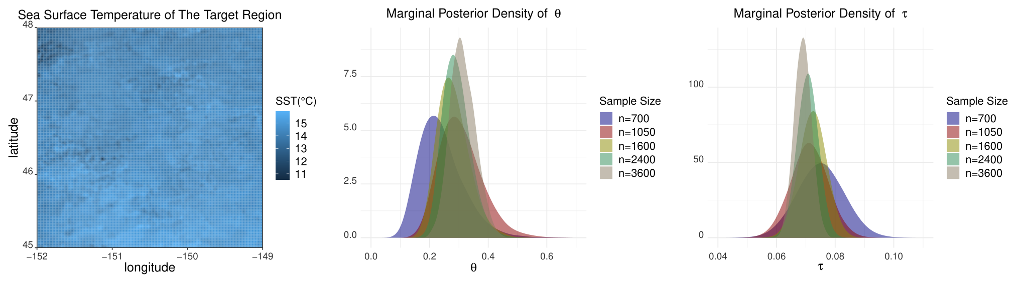
For a real data analysis, we fit Model (1) and the isotropic Matérn covariance function (2) with ν=1/2\nu=1/2 to the sea surface temperature data on the Pacific Ocean between 45∘45^{\circ}–48∘48^{\circ} north latitudes and 149∘149^{\circ}–152∘152^{\circ} west longitudes on August 16, 2016. The data were collected from remote sensing satellites with a high-resolution on a 0.025∘×0.025∘0.025^{\circ}\times 0.025^{\circ} grid, and can be obtained from National Oceanographic Data Centres (NODC) World Ocean Database (https://www.ncei.noaa.gov/products/world-ocean-database). For Bayesian estimation, we use a total of 3600 observations on the 0.05∘×0.05∘0.05^{\circ}\times 0.05^{\circ} grid, and set the sample size n=700,1050,1600,2400,3600n=700,1050,1600,2400,3600. For each nn smaller than 3600, we randomly choose 10 subsets of data YnY_{n}. We set the regressors f⁡(𝐬)=(1,s1,s2)T\mathrm{f}(\mathbf{s})=(1,s_{1},s_{2})^{\mathrm{\scriptscriptstyle T}} for the latitude s1s_{1} and the longitude s2s_{2}. We assign the same prior as in Proposition 2 with hyperparameters a0=106a_{0}=10^{6}, a1=b1=a2=b2=0.1a_{1}=b_{1}=a_{2}=b_{2}=0.1, and μ=λ=1\mu=\lambda=1. We draw 40004000 posterior samples of (θ,α,τ)(\theta,\alpha,\tau) after 10001000 burnins for each of the 10 subsets, and then average the 10 marginal posterior distributions into one summary posterior distribution using the Wasserstein-2 barycenter (Li et al. 2017). Figure 4 presents the summary marginal posterior densities of θ\theta and τ\tau for n∈{700,1050,1600,2400,3600}n\in\{700,1050,1600,2400,3600\}. As nn increases, we can see the clear trend of posterior contraction for both θ\theta and τ\tau, and the posterior of τ\tau seems to contract faster than that of θ\theta.

Refer to caption
Figure 4: Sea surface temperature data. Left panel: Temperature in the target region. Middle panel: Marginal posterior densities of θ\theta with various sample size nn. Right panel: Marginal posterior densities of τ\tau with various sample size nn.

5 Discussion

The general fixed-domain posterior contraction theory developed in this paper can be potentially applied to many stationary covariance functions in spatial statistics. With the new evidence lower bound, we have effectively transformed the problem of finding posterior contraction rates to the problem of finding efficient frequentist estimators that satisfy the concentration inequalities with exponentially small tails as in Assumption 4.

There are many potential directions to extend the current work. First, for isotropic Matérn, our higher-order quadratic variation estimators deliver the explicit posterior contraction rates, though it remains unclear what is the optimal rate for the microergodic parameter θ\theta under our flexible stratified sampling design. It would be of further interest to find the limiting Bayesian posterior distribution of (θ,α,τ,β)(\theta,\alpha,\tau,\beta) and establish the posterior asymptotic normality for both θ\theta and the nugget τ\tau, similar to the Bayesian fixed-domain asymptotic theory for the model without nugget in Li 2022.

Second, we have assumed that the smoothness parameter ν\nu is fixed and known in our theory. Because the smoothness parameter ν\nu determines the degree of mean square differentiability of the random field, estimation of ν\nu has been an important and meanwhile challenging problem in the spatial literature. Recently, using the new higher-order quadratic variation method, Loh 2015, Loh et al. 2021, and Loh and Sun 2023 have proposed consistent estimators of ν\nu for irregularly spaced spatial data under fixed-domain asymptotics. In fact, our estimator of the microergodic parameter θ\theta in Section 3.1 is the same as the estimator in Loh et al. 2021 and Loh and Sun 2023 when ν\nu is assumed to be known. It requires further study whether we can include ν\nu as part of the unknown parameters in the Bayesian framework, and establish the posterior contraction for ν\nu based on the new estimators.

Third, the isotropic covariance function considered in this paper leads to the simplest spatial Gaussian process model for real data. To extend our method to anisotropic covariance functions or even nonstationary spatial processes, we need to both establish the evidence lower bound similar to Theorem 1 and find some consistent frequentist estimators for the microergodic parameters in these more general covariance functions under fixed-domain asymptotics. From the technical perspective, it seems that finding consistent estimators will be a more challenging task than deriving the evidence lower bound, though both of them may require a case-by-case analysis for different spatial covariance functions. Meanwhile, it is possible to adapt the current proof techniques to a general nonparametric class of covariance functions based the principal irregular terms in their Taylor expansions (see Section 2.7 of Stein 1999), in a similar spirit to the recent work Bachoc and Lagnoux 2020.

Fourth, given the frequentist asymptotic efficiency in Stein 1990a; Stein 1990b for Gaussian processes without nugget as well as our promising simulation results, it would be of theoretical interest to show that the asymptotic efficiency can still be preserved even in the Bayesian posterior prediction for the true mean function Y0​(𝐬)=β0T​f​(𝐬)+X⁡(𝐬)Y_{0}(\mathbf{s})=\beta_{0}^{\mathrm{\scriptscriptstyle T}}\mathrm{f}(\mathbf{s})+X(\mathbf{s}) in the more general model (1) with both regression terms and nugget.

These potential developments will together provide strong theoretical justification for the existing Bayesian spatial inference based on the Gaussian process regression model, including parameter estimation, uncertainty quantification, and prediction. We leave these directions for future research.

Acknowledgements

The authors thank Professor Wei-Liem Loh for helpful discussion. This work was supported by Singapore Ministry of Education Academic Research Funds Tier 1 Grant A-0004822-00-00.

Supplementary Material

Supplementary Material for “Fixed-domain Posterior Contraction Rates for Spatial Gaussian Process Model with Nugget”: Technical proofs of all theorems, propositions, and additional simulation results.

Supplementary Material for “Fixed-domain Posterior Contraction Rates for Spatial Gaussian Process Model with Nugget”

This supplementary material contains the technical proofs of the theorems and propositions in the main paper as well as additional simulation results. Section S1 contains the proof of Theorem 2. Section S2 contains the proof of Theorem 1 and auxiliary technical results on spectral analysis. Section S3 proves a proposition on the posterior inconsistency of the range parameter α\alpha and the regression coefficient vector β\beta. Sections S4, S5, and S6 include the proofs of Proposition 1, Theorem 4, and Proposition 2, respectively. Section S7 contains the lengthy proof of Theorem 3. Section S8 includes the formulas for calculating the Bayesian and oracle prediction mean squared errors for Model (1) in the main text and additional simulation results for the case of domain dimension d=1d=1.

We define some universal notation that will be used throughout the proof. Let ℝ+=(0,+∞)\mathbb{R}_{+}=(0,+\infty), ℤ+\mathbb{Z}_{+} be the set of all positive integers, and ℕ=ℤ+∪{0}\mathbb{N}=\mathbb{Z}_{+}\cup\{0\}. For any x∈ℝx\in\mathbb{R}, ⌈x⌉\lceil x\rceil and ⌊x⌋\lfloor x\rfloor denote the smallest integer ≥x\geq x and the largest integer ≤x\leq x. For any x=(x1,…,xd)T∈ℝdx=(x_{1},\ldots,x_{d})^{\mathrm{\scriptscriptstyle T}}\in\mathbb{R}^{d}, we let ‖x‖=(∑i=1dxi2)1/2\|x\|=\big(\sum_{i=1}^{d}x_{i}^{2}\big)^{1/2}, ‖x‖1=∑i=1d|xi|\|x\|_{1}=\sum_{i=1}^{d}|x_{i}|, and ‖x‖∞=max⁡(x1,…,xd)\|x\|_{\infty}=\max(x_{1},\ldots,x_{d}). For a generic set ℰ\Ecal, we use ℰc\Ecal^{c} to denote its complement. If ℰ\Ecal contains finitely many elements, then |ℰ||\Ecal| denotes its cardinality.

For two positive sequences ana_{n} and bnb_{n}, we use an≺bna_{n}\prec b_{n} and bn≻anb_{n}\succ a_{n} to denote the relation limn→∞an/bn=0\lim_{n\to\infty}a_{n}/b_{n}=0. an=O⁡(bn)a_{n}=O(b_{n}), an⪯bna_{n}\preceq b_{n} and bn⪰anb_{n}\succeq a_{n} denote the relation lim supn→∞an/bn<+∞\limsup_{n\to\infty}a_{n}/b_{n}<+\infty. an≍bna_{n}\asymp b_{n} denotes the relation an⪯bna_{n}\preceq b_{n} and an⪰bna_{n}\succeq b_{n}.

For any integers k,mk,m, we let IkI_{k} be the k×kk\times k identity matrix, 0k0_{k} be the kk-dimensional column vectors of all zeros, 0k×m0_{k\times m} be the k×mk\times m zero matrix, and diag{c1,…,ck}\diag\{c_{1},\ldots,c_{k}\} be the diagonal matrix with diagonal entries c1,…,ck∈ℝc_{1},\ldots,c_{k}\in\mathbb{R}. For any generic matrix AA, c​AcA denotes the matrix of AA with all entries multiplied by the number cc, and det(A)\dett(A) denotes the determinant of AA. For a square matrix AA, tr(A)\tr(A) denotes the trace of AA. If AA is symmetric positive semidefinite, then 𝗌min​(A)\mathsf{s}_{\min}(A) and 𝗌max​(A)\mathsf{s}_{\max}(A) denote the smallest and largest eigenvalues of AA, and A1/2A^{1/2} denotes a symmetric positive semidefinite square root of AA. For two symmetric matrices AA and BB, we use A⪯BA\preceq B and B⪰AB\succeq A to denote the relation that B−AB-A is symmetric positive semidefinite, and use A≺BA\prec B and B≻AB\succ A to denote the relation that B−AB-A is symmetric positive definite. For any matrix AA, ‖A‖op={𝗌max​(AT​A)}1/2={𝗌max​(A​AT)}1/2\|A\|_{\op}=\big\{\mathsf{s}_{\max}(A^{\mathrm{\scriptscriptstyle T}}A)\big\}^{1/2}=\big\{\mathsf{s}_{\max}(AA^{\mathrm{\scriptscriptstyle T}})\big\}^{1/2} denotes the operator norm of AA, and ‖A‖F={tr(AT​A)}1/2\|A\|_{F}=\big\{\tr\left(A^{\mathrm{\scriptscriptstyle T}}A\right)\big\}^{1/2} denotes the Frobenius norm of AA. We use Pr(⋅)\pr(\cdot) to denote the probability under the probability measure ℙ(θ0,α0,τ0,β0)\mathbb{P}_{(\theta_{0},\alpha_{0},\tau_{0},\beta_{0})}.

S1 Proof of Theorem 2

Proof.

We first show the propriety of the posterior distribution defined in Equation (6) of the main text, which is equivalent to showing that the integral in the denominator on the right-hand side of (6) is finite. Since for two positive definite matrices AA and BB, det(A+B)≥det(A)\dett(A+B)\geq\dett(A), we have that for any given n∈ℤ+n\in\mathbb{Z}_{+},

∫ℝ+3×ℝpexp⁡{ℒn⁡(θ,α,τ,β)}​π​(θ,α,τ,β)​𝑑θ​𝑑τ​𝑑α​𝑑β\displaystyle\quad~\int_{\mathbb{R}_{+}^{3}\times\mathbb{R}^{p}}\exp\left\{\Lcal_{n}(\theta,\alpha,\tau,\beta)\right\}\pi(\theta,\alpha,\tau,\beta)\mathrm{d}\theta\mathrm{d}\tau\mathrm{d}\alpha\mathrm{d}\beta
=∫ℝ+3×ℝp1[det{θ​Kα,ν​(Sn)+τ​In}]1/2​exp⁡{−12​(Yn−Fn​β)T​{θ​Kα,ν​(Sn)+τ​In}−1​(Yn−Fn​β)}\displaystyle=\int_{\mathbb{R}_{+}^{3}\times\mathbb{R}^{p}}\frac{1}{\left[\dett\left\{\theta K_{\alpha,\nu}(S_{n})+\tau I_{n}\right\}\right]^{1/2}}\exp\left\{-\frac{1}{2}(Y_{n}-F_{n}\beta)^{\mathrm{\scriptscriptstyle T}}\left\{\theta K_{\alpha,\nu}(S_{n})+\tau I_{n}\right\}^{-1}(Y_{n}-F_{n}\beta)\right\}
×π⁡(θ,α,τ,β)​d​θ​d​τ​d​α​d​β\displaystyle\qquad\times\pi(\theta,\alpha,\tau,\beta)\mathrm{d}\theta\mathrm{d}\tau\mathrm{d}\alpha\mathrm{d}\beta
≤∫ℝ+3×ℝp1{det(τ​In)}1/2⋅1⋅π⁡(θ,α,τ,β)​𝑑θ​𝑑τ​𝑑α​𝑑β\displaystyle\leq\int_{\mathbb{R}_{+}^{3}\times\mathbb{R}^{p}}\frac{1}{\left\{\dett(\tau I_{n})\right\}^{1/2}}\cdot 1\cdot\pi(\theta,\alpha,\tau,\beta)\mathrm{d}\theta\mathrm{d}\tau\mathrm{d}\alpha\mathrm{d}\beta
=∫0∞τ−n/2π(τ)dτ<∞,\displaystyle=\int_{0}^{\infty}\tau^{-n/2}\pi(\tau)\mathrm{d}\tau<\infty,

where the last integral is finite following Assumption 3. This proves that the joint posterior density π(θ,α,τ,β|Yn,Fn)\pi(\theta,\alpha,\tau,\beta~|~Y_{n},F_{n}) in Equation (6) is well defined.

Next, we prove the posterior contraction rates for θ\theta and τ\tau in Theorem 2. We follow the classical proof of the Schwartz’s theorem for posterior consistency (Schwartz 1965); see for example, Theorem 6.17 in Ghosal and van der Vaart 2017. Let ε1​n=Mn​n−b1​log⁡n\varepsilon_{1n}=M_{n}n^{-b_{1}}\log n and ε2​n=Mn​n−b2​log⁡n\varepsilon_{2n}=M_{n}n^{-b_{2}}\log n. Define the testing function

ϕn\displaystyle\phi_{n} =ℐ⁡(|θ^n/θ0−1|≥ε1​n/2, or ​|τ^n/τ0−1|≥ε2​n/2),\displaystyle=\Ical\left(|\widehat{\theta}_{n}/\theta_{0}-1|\geq\varepsilon_{1n}/2,\text{ or }|\widehat{\tau}_{n}/\tau_{0}-1|\geq\varepsilon_{2n}/2\right), (S.1)

where θ^n\widehat{\theta}_{n} and τ^n\widehat{\tau}_{n} are from Assumption 4.

We start with the decomposition

Π⁡(ℬ0⁡(ε1​n,ε2​n)c|Yn,Fn)=∫ℬ0⁡(ε1​n,ε2​n)cexp⁡{ℒn⁡(θ,α,τ,β)}​π​(θ,α,τ,β)​𝑑θ​𝑑τ​𝑑α​𝑑β∫ℝ+3×ℝpexp⁡{ℒn⁡(θ′,α′,τ′,β′)}​π​(θ′,α′,τ′,β′)​d​θ′​d​τ′​d​α′​d​β′\displaystyle\Pi\left(\Bcal_{0}(\varepsilon_{1n},\varepsilon_{2n})^{c}~|~Y_{n},F_{n}\right)=\frac{\int_{\Bcal_{0}(\varepsilon_{1n},\varepsilon_{2n})^{c}}\exp\left\{\Lcal_{n}(\theta,\alpha,\tau,\beta)\right\}\pi(\theta,\alpha,\tau,\beta)\mathrm{d}\theta\mathrm{d}\tau\mathrm{d}\alpha\mathrm{d}\beta}{\int_{\mathbb{R}_{+}^{3}\times\mathbb{R}^{p}}\exp\left\{\Lcal_{n}(\theta^{\prime},\alpha^{\prime},\tau^{\prime},\beta^{\prime})\right\}\pi(\theta^{\prime},\alpha^{\prime},\tau^{\prime},\beta^{\prime})\mathrm{d}\theta^{\prime}\mathrm{d}\tau^{\prime}\mathrm{d}\alpha^{\prime}\mathrm{d}\beta^{\prime}}
≤ϕn+(1−ϕn)​∫ℬ0⁡(ε1​n,ε2​n)cexp⁡{ℒn⁡(θ,α,τ,β)}​π​(θ,α,τ,β)​𝑑θ​𝑑τ​𝑑α​𝑑β∫ℝ+3×ℝpexp⁡{ℒn⁡(θ′,α′,τ′,β′)}​π​(θ′,α′,τ′,β′)​d​θ′​d​τ′​d​α′​d​β′.\displaystyle\leq\phi_{n}+\frac{(1-\phi_{n})\int_{\Bcal_{0}(\varepsilon_{1n},\varepsilon_{2n})^{c}}\exp\left\{\Lcal_{n}(\theta,\alpha,\tau,\beta)\right\}\pi(\theta,\alpha,\tau,\beta)\mathrm{d}\theta\mathrm{d}\tau\mathrm{d}\alpha\mathrm{d}\beta}{\int_{\mathbb{R}_{+}^{3}\times\mathbb{R}^{p}}\exp\left\{\Lcal_{n}(\theta^{\prime},\alpha^{\prime},\tau^{\prime},\beta^{\prime})\right\}\pi(\theta^{\prime},\alpha^{\prime},\tau^{\prime},\beta^{\prime})\mathrm{d}\theta^{\prime}\mathrm{d}\tau^{\prime}\mathrm{d}\alpha^{\prime}\mathrm{d}\beta^{\prime}}. (S.2)

By Assumption 4, we have that for some large positive constant N0N_{0}, for all n>N0n>N_{0},

𝔼(θ0,α0,τ0,β0)​(ϕn)\displaystyle{\mathbb{E}}_{(\theta_{0},\alpha_{0},\tau_{0},\beta_{0})}(\phi_{n}) ≤exp⁡{−c1​φ​(nb1​ε1​n)}+exp⁡{−c2​φ​(nb2​ε2​n)}\displaystyle\leq\exp\left\{-c_{1}\varphi\left(n^{b_{1}}\varepsilon_{1n}\right)\right\}+\exp\left\{-c_{2}\varphi\left(n^{b_{2}}\varepsilon_{2n}\right)\right\}
≤exp⁡(−c1​Mn​log⁡n)+exp⁡(−c2​Mn​log⁡n)→0,\displaystyle\leq\exp\left(-c_{1}M_{n}\log n\right)+\exp\left(-c_{2}M_{n}\log n\right)\to 0,

where the last step follows from Mn→+∞M_{n}\to+\infty as n→∞n\to\infty. Notice that for any constant c>0c>0 and an arbitrary c′>1c^{\prime}>1, exp⁡(−c​Mn​log⁡n)≤exp⁡(−c′​log⁡n)=n−c′\exp\left(-cM_{n}\log n\right)\leq\exp(-c^{\prime}\log n)=n^{-c^{\prime}} for all sufficiently large nn and hence the sequence exp⁡(−c​Mn​log⁡n)\exp\left(-cM_{n}\log n\right) is summable over nn. Therefore, by the Markov’s inequality and the Borel-Cantelli lemma, ϕn→0\phi_{n}\to 0 almost surely ℙ(θ0,α0,τ0)\mathbb{P}_{(\theta_{0},\alpha_{0},\tau_{0})} as n→∞n\to\infty.

We now turn to the second term in (S1). It can be further decomposed into two terms:

(1−ϕn)​∫ℬ0⁡(ε1​n,ε2​n)cexp⁡{ℒn⁡(θ,α,τ,β)}​π​(θ,α,τ,β)​𝑑θ​𝑑τ​𝑑α​𝑑β∫ℝ+3×ℝpexp⁡{ℒn⁡(θ′,α′,τ′,β′)}​π​(θ′,α′,τ′,β′)​d​θ′​d​τ′​d​α′​d​β′=T1+T2, where\displaystyle\frac{(1-\phi_{n})\int_{\Bcal_{0}(\varepsilon_{1n},\varepsilon_{2n})^{c}}\exp\left\{\Lcal_{n}(\theta,\alpha,\tau,\beta)\right\}\pi(\theta,\alpha,\tau,\beta)\mathrm{d}\theta\mathrm{d}\tau\mathrm{d}\alpha\mathrm{d}\beta}{\int_{\mathbb{R}_{+}^{3}\times\mathbb{R}^{p}}\exp\left\{\Lcal_{n}(\theta^{\prime},\alpha^{\prime},\tau^{\prime},\beta^{\prime})\right\}\pi(\theta^{\prime},\alpha^{\prime},\tau^{\prime},\beta^{\prime})\mathrm{d}\theta^{\prime}\mathrm{d}\tau^{\prime}\mathrm{d}\alpha^{\prime}\mathrm{d}\beta^{\prime}}=T_{1}+T_{2},\quad\text{ where }
T1=(1−ϕn)​∫ℬ0⁡(ε1​n,ε2​n)c∩ℰnexp⁡{ℒn⁡(θ,α,τ,β)−ℒn⁡(θ0,α0,τ0,β0)}​π​(θ,α,τ,β)​𝑑θ​𝑑τ​𝑑α​𝑑β∫ℝ+3×ℝpexp⁡{ℒn⁡(θ′,α′,τ′,β′)−ℒn⁡(θ0,α0,τ0,β0)}​π​(θ′,α′,τ′,β′)​d​θ′​d​τ′​d​α′​d​β′,\displaystyle T_{1}=\frac{(1-\phi_{n})\int_{\Bcal_{0}(\varepsilon_{1n},\varepsilon_{2n})^{c}\cap\Ecal_{n}}\exp\left\{\Lcal_{n}(\theta,\alpha,\tau,\beta)-\Lcal_{n}(\theta_{0},\alpha_{0},\tau_{0},\beta_{0})\right\}\pi(\theta,\alpha,\tau,\beta)\mathrm{d}\theta\mathrm{d}\tau\mathrm{d}\alpha\mathrm{d}\beta}{\int_{\mathbb{R}_{+}^{3}\times\mathbb{R}^{p}}\exp\left\{\Lcal_{n}(\theta^{\prime},\alpha^{\prime},\tau^{\prime},\beta^{\prime})-\Lcal_{n}(\theta_{0},\alpha_{0},\tau_{0},\beta_{0})\right\}\pi(\theta^{\prime},\alpha^{\prime},\tau^{\prime},\beta^{\prime})\mathrm{d}\theta^{\prime}\mathrm{d}\tau^{\prime}\mathrm{d}\alpha^{\prime}\mathrm{d}\beta^{\prime}},
T2=(1−ϕn)​∫ℬ0⁡(ε1​n,ε2​n)c∩ℰncexp⁡{ℒn⁡(θ,α,τ,β)−ℒn⁡(θ0,α0,τ0,β0)}​π​(θ,α,τ,β)​𝑑θ​𝑑τ​𝑑α​𝑑β∫ℝ+3×ℝpexp⁡{ℒn⁡(θ′,α′,τ′,β′)−ℒn⁡(θ0,α0,τ0,β0)}​π​(θ′,α′,τ′,β′)​d​θ′​d​τ′​d​α′​d​β′.\displaystyle T_{2}=\frac{(1-\phi_{n})\int_{\Bcal_{0}(\varepsilon_{1n},\varepsilon_{2n})^{c}\cap\Ecal_{n}^{c}}\exp\left\{\Lcal_{n}(\theta,\alpha,\tau,\beta)-\Lcal_{n}(\theta_{0},\alpha_{0},\tau_{0},\beta_{0})\right\}\pi(\theta,\alpha,\tau,\beta)\mathrm{d}\theta\mathrm{d}\tau\mathrm{d}\alpha\mathrm{d}\beta}{\int_{\mathbb{R}_{+}^{3}\times\mathbb{R}^{p}}\exp\left\{\Lcal_{n}(\theta^{\prime},\alpha^{\prime},\tau^{\prime},\beta^{\prime})-\Lcal_{n}(\theta_{0},\alpha_{0},\tau_{0},\beta_{0})\right\}\pi(\theta^{\prime},\alpha^{\prime},\tau^{\prime},\beta^{\prime})\mathrm{d}\theta^{\prime}\mathrm{d}\tau^{\prime}\mathrm{d}\alpha^{\prime}\mathrm{d}\beta^{\prime}}. (S.3)

For the first term T1T_{1} in (S1), by Assumption 4 and the Fubini’s theorem, the numerator has expectation

𝔼(θ0,α0,τ0,β0)(1−ϕn)∫ℬ0⁡(ε1​n,ε2​n)c∩ℰnexp{ℒn(θ,α,τ,β)\displaystyle{\mathbb{E}}_{(\theta_{0},\alpha_{0},\tau_{0},\beta_{0})}(1-\phi_{n})\int_{\Bcal_{0}(\varepsilon_{1n},\varepsilon_{2n})^{c}\cap\Ecal_{n}}\exp\Big\{\Lcal_{n}(\theta,\alpha,\tau,\beta)
−ℒn(θ0,α0,τ0,β0)}π(θ,α,τ,β)dθdτdαdβ\displaystyle~~-\Lcal_{n}(\theta_{0},\alpha_{0},\tau_{0},\beta_{0})\Big\}\pi(\theta,\alpha,\tau,\beta)\mathrm{d}\theta\mathrm{d}\tau\mathrm{d}\alpha\mathrm{d}\beta
=\displaystyle={} ∫ℬ0⁡(ε1​n,ε2​n)c∩ℰn𝔼(θ,α,τ,β)​(1−ϕn)​π​(θ,α,τ,β)​𝑑θ​𝑑τ​𝑑α​𝑑β\displaystyle\int_{\Bcal_{0}(\varepsilon_{1n},\varepsilon_{2n})^{c}\cap\Ecal_{n}}{\mathbb{E}}_{(\theta,\alpha,\tau,\beta)}(1-\phi_{n})\pi(\theta,\alpha,\tau,\beta)\mathrm{d}\theta\mathrm{d}\tau\mathrm{d}\alpha\mathrm{d}\beta
≤\displaystyle\leq{} supℬ0⁡(ε1​n,ε2​n)c∩ℰn𝔼(θ,α,τ,β)​{(1−ϕn)⋅∫ℬ0⁡(ϵ1,ϵ2)c∩ℰnπ⁡(θ,α,τ,β)​𝑑θ​𝑑τ​𝑑α​𝑑β}\displaystyle\sup_{\Bcal_{0}(\varepsilon_{1n},\varepsilon_{2n})^{c}\cap\Ecal_{n}}{\mathbb{E}}_{(\theta,\alpha,\tau,\beta)}\left\{(1-\phi_{n})\cdot\int_{\Bcal_{0}(\epsilon_{1},\epsilon_{2})^{c}\cap\Ecal_{n}}\pi(\theta,\alpha,\tau,\beta)\mathrm{d}\theta\mathrm{d}\tau\mathrm{d}\alpha\mathrm{d}\beta\right\}
≤\displaystyle\leq{} supℬ0⁡(ε1​n,ε2​n)c∩ℰn𝔼(θ,α,τ,β)​(1−ϕn)\displaystyle\sup_{\Bcal_{0}(\varepsilon_{1n},\varepsilon_{2n})^{c}\cap\Ecal_{n}}{\mathbb{E}}_{(\theta,\alpha,\tau,\beta)}(1-\phi_{n})
≤\displaystyle\leq{} supℬ0⁡(ε1​n,ε2​n)c∩ℰnℙ(θ,α,τ,β)​(|θ^n/θ0−1|≤ε1​n/2)+supℬ0⁡(ε1​n,ε2​n)c∩ℰnℙ(θ,α,τ,β)​(|τ^n/τ0−1|≤ε2​n/2)\displaystyle\sup_{\Bcal_{0}(\varepsilon_{1n},\varepsilon_{2n})^{c}\cap\Ecal_{n}}\mathbb{P}_{(\theta,\alpha,\tau,\beta)}\left(|\widehat{\theta}_{n}/\theta_{0}-1|\leq\varepsilon_{1n}/2\right)+\sup_{\Bcal_{0}(\varepsilon_{1n},\varepsilon_{2n})^{c}\cap\Ecal_{n}}\mathbb{P}_{(\theta,\alpha,\tau,\beta)}\left(|\widehat{\tau}_{n}/\tau_{0}-1|\leq\varepsilon_{2n}/2\right)
≤\displaystyle\leq{} exp⁡{−c1​φ​(nb1​ε1​n)}+exp⁡{−c2​φ​(nb2​ε2​n)}\displaystyle\exp\left\{-c_{1}\varphi\left(n^{b_{1}}\varepsilon_{1n}\right)\right\}+\exp\left\{-c_{2}\varphi\left(n^{b_{2}}\varepsilon_{2n}\right)\right\}
=\displaystyle={} exp⁡(−c1​Mn​log⁡n)+exp⁡(−c2​Mn​log⁡n).\displaystyle\exp\left(-c_{1}M_{n}\log n\right)+\exp\left(-c_{2}M_{n}\log n\right). (S.4)

Therefore, by applying the Markov’s inequality and the Borel-Cantelli Lemma to (S1), the numerator of T1T_{1} in (S1) is smaller than exp{−min(c1,c2)Mnlogn/2}\exp\left\{-\min(c_{1},c_{2})M_{n}\log n/2\right\} almost surely ℙ(θ0,α0,τ0,β0)\mathbb{P}_{(\theta_{0},\alpha_{0},\tau_{0},\beta_{0})} as n→∞n\to\infty. On the other hand, Theorem 1 shows that almost surely ℙ(θ0,α0,τ0,β0)\mathbb{P}_{(\theta_{0},\alpha_{0},\tau_{0},\beta_{0})} as n→∞n\to\infty, for all d∈ℤ+d\in\mathbb{Z}_{+}, the denominator in T1T_{1} in (S1) is lower bounded by

∫ℝ+3×ℝpexp⁡{ℒn⁡(θ′,α′,τ′,β′)−ℒn⁡(θ0,α0,τ0,β0)}\displaystyle\int_{\mathbb{R}_{+}^{3}\times\mathbb{R}^{p}}\exp\left\{\Lcal_{n}(\theta^{\prime},\alpha^{\prime},\tau^{\prime},\beta^{\prime})-\Lcal_{n}(\theta_{0},\alpha_{0},\tau_{0},\beta_{0})\right\}
×π⁡(θ′,α′,τ′,β′)​d​θ′​d​τ′​d​α′​d​β′≥D​n−(3​p+2+2/κ),\displaystyle~~\times\pi(\theta^{\prime},\alpha^{\prime},\tau^{\prime},\beta^{\prime})\mathrm{d}\theta^{\prime}\mathrm{d}\tau^{\prime}\mathrm{d}\alpha^{\prime}\mathrm{d}\beta^{\prime}\geq Dn^{-(3p+2+2/\kappa)}, (S.5)

for some constant D>0D>0. Hence for all sufficiently large nn, the first term T1T_{1} in (S1) is upper bounded by

T1\displaystyle T_{1} ≤D−1n(3​p+2+2/κ)exp{−min(c1,c2)Mnlogn/2}≤exp(−c′logn)→0,\displaystyle\leq D^{-1}n^{(3p+2+2/\kappa)}\exp\left\{-\min(c_{1},c_{2})M_{n}\log n/2\right\}\leq\exp(-c^{\prime}\log n)\to 0, (S.6)

for an arbitrary c′>1c^{\prime}>1, almost surely ℙ(θ0,α0,τ0,β0)\mathbb{P}_{(\theta_{0},\alpha_{0},\tau_{0},\beta_{0})}.

For the second term T2T_{2} in (S1), by Assumption 4 and the Fubini’s theorem, the numerator has expectation

𝔼(θ0,α0,τ0,β0)(1−ϕn)∫ℬ0⁡(ε1​n,ε2​n)c∩ℰncexp{ℒn(θ,α,τ,β)\displaystyle{\mathbb{E}}_{(\theta_{0},\alpha_{0},\tau_{0},\beta_{0})}(1-\phi_{n})\int_{\Bcal_{0}(\varepsilon_{1n},\varepsilon_{2n})^{c}\cap\Ecal_{n}^{c}}\exp\Big\{\Lcal_{n}(\theta,\alpha,\tau,\beta)
−ℒn(θ0,α0,τ0,β0)}π(θ,α,τ,β)dθdτdαdβ\displaystyle\quad-\Lcal_{n}(\theta_{0},\alpha_{0},\tau_{0},\beta_{0})\Big\}\pi(\theta,\alpha,\tau,\beta)\mathrm{d}\theta\mathrm{d}\tau\mathrm{d}\alpha\mathrm{d}\beta
=\displaystyle={} ∫ℬ0⁡(ε1​n,ε2​n)c∩ℰnc𝔼(θ0,α0,τ0,β0)(1−ϕn)exp{ℒn(θ,α,τ,β)\displaystyle\int_{\Bcal_{0}(\varepsilon_{1n},\varepsilon_{2n})^{c}\cap\Ecal_{n}^{c}}{\mathbb{E}}_{(\theta_{0},\alpha_{0},\tau_{0},\beta_{0})}(1-\phi_{n})\exp\Big\{\Lcal_{n}(\theta,\alpha,\tau,\beta)
−ℒn(θ0,α0,τ0,β0)}π(θ,α,τ,β)dθdτdαdβ\displaystyle\quad-\Lcal_{n}(\theta_{0},\alpha_{0},\tau_{0},\beta_{0})\Big\}\pi(\theta,\alpha,\tau,\beta)\mathrm{d}\theta\mathrm{d}\tau\mathrm{d}\alpha\mathrm{d}\beta
=\displaystyle={} ∫ℬ0⁡(ε1​n,ε2​n)c∩ℰnc𝔼(θ,α,τ,β)​(1−ϕn)​π​(θ,α,τ,β)​𝑑θ​𝑑τ​𝑑α​𝑑β\displaystyle\int_{\Bcal_{0}(\varepsilon_{1n},\varepsilon_{2n})^{c}\cap\Ecal_{n}^{c}}{\mathbb{E}}_{(\theta,\alpha,\tau,\beta)}(1-\phi_{n})\pi(\theta,\alpha,\tau,\beta)\mathrm{d}\theta\mathrm{d}\tau\mathrm{d}\alpha\mathrm{d}\beta
≤\displaystyle\leq{} ∫ℰnc1⋅π⁡(θ,α,τ,β)​𝑑θ​𝑑τ​𝑑α​𝑑β=Π⁡(ℰnc)≤n−(3​p+4+2/κ).\displaystyle\int_{\Ecal_{n}^{c}}1\cdot\pi(\theta,\alpha,\tau,\beta)\mathrm{d}\theta\mathrm{d}\tau\mathrm{d}\alpha\mathrm{d}\beta=\Pi(\Ecal_{n}^{c})\leq n^{-(3p+4+2/\kappa)}. (S.7)

Therefore, by applying the Markov’s inequality to (S1), the numerator of T2T_{2} in (S1) is smaller than n−(3​p+52+2κ)n^{-\left(3p+\frac{5}{2}+\frac{2}{\kappa}\right)} with probability at least 1−n−3/21-n^{-3/2}. Since the sequence {n−3/2:n≥1}\{n^{-3/2}:n\geq 1\} is summable over nn, by the Borel-Cantelli Lemma, we have that the numerator of T2T_{2} in (S1) is smaller than n−(3​p+52+2κ)n^{-\left(3p+\frac{5}{2}+\frac{2}{\kappa}\right)} almost surely ℙ(θ0,α0,τ0,β0)\mathbb{P}_{(\theta_{0},\alpha_{0},\tau_{0},\beta_{0})} as n→∞n\to\infty. We combine this with the lower bound in (S1) to conclude that almost surely ℙ(θ0,α0,τ0,β0)\mathbb{P}_{(\theta_{0},\alpha_{0},\tau_{0},\beta_{0})} as n→∞n\to\infty, the second term T2T_{2} in (S1) is upper bounded by

T2\displaystyle T_{2} ≤D−1n3​p+2+2/κ⋅n−(3​p+52+2κ)=D−1n−1/2→0.\displaystyle\leq D^{-1}n^{3p+2+2/\kappa}\cdot n^{-\left(3p+\frac{5}{2}+\frac{2}{\kappa}\right)}=D^{-1}n^{-1/2}\to 0. (S.8)

Finally, we combine (S1), (S1), (S.6), and (S.8) to conclude that the right-hand side of (S1) converges to zero almost surely ℙ(θ0,α0,τ0,β0)\mathbb{P}_{(\theta_{0},\alpha_{0},\tau_{0},\beta_{0})} as n→∞n\to\infty, which completes the proof of Theorem 2. ∎

S2 Proof of Theorems 1 and Auxiliary Technical Lemmas

S2.1 Proof of Theorem 1

Proof.

Define the sets 𝒜n\Acal_{n} and 𝒟n\Dcal_{n} as

𝒜n={(θ,α,τ,β)∈ℝ+3×ℝp:|α/α0−1|≤n−2/κ},\displaystyle\Acal_{n}=\left\{(\theta,\alpha,\tau,\beta)\in\mathbb{R}_{+}^{3}\times\mathbb{R}^{p}:~|\alpha/\alpha_{0}-1|\leq n^{-2/\kappa}\right\},
𝒟n={(θ,α,τ,β)∈ℝ+3×ℝp:‖β−β0‖≤n−3}.\displaystyle\Dcal_{n}=\left\{(\theta,\alpha,\tau,\beta)\in\mathbb{R}_{+}^{3}\times\mathbb{R}^{p}:~\|\beta-\beta_{0}\|\leq n^{-3}\right\}.

By the continuity of the prior density in Assumption 3, we have that for all sufficiently large nn, π⁡(θ,τ,α,β)>π⁡(θ0,τ0,α0,β0)/2>0\pi(\theta,\tau,\alpha,\beta)>\pi(\theta_{0},\tau_{0},\alpha_{0},\beta_{0})/2>0 for all (θ,τ,α,β)∈ℬ0⁡(n−1,n−1)∩𝒜n∩𝒟n(\theta,\tau,\alpha,\beta)\in\Bcal_{0}(n^{-1},n^{-1})\cap\Acal_{n}\cap\Dcal_{n}. Therefore,

Π⁡(ℬ0⁡(n−1,n−1)∩𝒜n∩𝒟n)\displaystyle\Pi\left(\Bcal_{0}(n^{-1},n^{-1})\cap\Acal_{n}\cap\Dcal_{n}\right) ≥π⁡(θ0,τ0,α0,β0)2⋅(2θ0n−1)⋅(2τ0n−1)⋅(2α0n−2/κ)⋅v0n−3​p\displaystyle\geq\frac{\pi(\theta_{0},\tau_{0},\alpha_{0},\beta_{0})}{2}\cdot(2\theta_{0}n^{-1})\cdot(2\tau_{0}n^{-1})\cdot(2\alpha_{0}n^{-2/\kappa})\cdot v_{0}n^{-3p}
=4​v0​θ0​τ0​α0​π​(θ0,τ0,α0,β0)​n−(3​p+2+2/κ),\displaystyle=4v_{0}\theta_{0}\tau_{0}\alpha_{0}\pi(\theta_{0},\tau_{0},\alpha_{0},\beta_{0})n^{-(3p+2+2/\kappa)}, (S.9)

where v0=πp/2/Γ⁡(p/2+1)v_{0}=\pi^{p/2}/\Gamma(p/2+1). Using the definition of log-likelihood in (2), the exponent in Theorem 1 can be written as

ℒn⁡(θ,α,τ,β)−ℒn⁡(θ0,α0,τ0,β0)\displaystyle\Lcal_{n}(\theta,\alpha,\tau,\beta)-\Lcal_{n}(\theta_{0},\alpha_{0},\tau_{0},\beta_{0})
=\displaystyle={} −12​{tr[{θ​Kα,ν​(Sn)+τ​In}−1​Y~n​Y~nT]−tr[{θ0​Kα0,ν​(Sn)+τ0​In}−1​Y~n​Y~nT]}\displaystyle-\frac{1}{2}\left\{\tr\left[\left\{\theta K_{\alpha,\nu}(S_{n})+\tau I_{n}\right\}^{-1}\widetilde{Y}_{n}\widetilde{Y}_{n}^{\mathrm{\scriptscriptstyle T}}\right]-\tr\left[\left\{\theta_{0}K_{\alpha_{0},\nu}(S_{n})+\tau_{0}I_{n}\right\}^{-1}\widetilde{Y}_{n}\widetilde{Y}_{n}^{\mathrm{\scriptscriptstyle T}}\right]\right\}
−12​log⁡det{θ​Kα,ν​(Sn)+τ​In}det{θ0​Kα0,ν​(Sn)+τ0​In}\displaystyle-\frac{1}{2}\log\frac{\dett\left\{\theta K_{\alpha,\nu}(S_{n})+\tau I_{n}\right\}}{\dett\left\{\theta_{0}K_{\alpha_{0},\nu}(S_{n})+\tau_{0}I_{n}\right\}}
+Y~nT​[{θ​Kα,ν​(Sn)+τ​In}−1−{θ0​Kα0,ν​(Sn)+τ0​In}−1]​Fn​(β−β0)\displaystyle+\widetilde{Y}_{n}^{\mathrm{\scriptscriptstyle T}}\left[\left\{\theta K_{\alpha,\nu}(S_{n})+\tau I_{n}\right\}^{-1}-\left\{\theta_{0}K_{\alpha_{0},\nu}(S_{n})+\tau_{0}I_{n}\right\}^{-1}\right]F_{n}(\beta-\beta_{0})
−12​(β−β0)T​FnT​[{θ​Kα,ν​(Sn)+τ​In}−1−{θ0​Kα0,ν​(Sn)+τ0​In}−1]​Fn​(β−β0).\displaystyle-\frac{1}{2}(\beta-\beta_{0})^{\mathrm{\scriptscriptstyle T}}F_{n}^{\mathrm{\scriptscriptstyle T}}\left[\left\{\theta K_{\alpha,\nu}(S_{n})+\tau I_{n}\right\}^{-1}-\left\{\theta_{0}K_{\alpha_{0},\nu}(S_{n})+\tau_{0}I_{n}\right\}^{-1}\right]F_{n}(\beta-\beta_{0}).

Using the lower bounds in Part (i) of Lemma S.5 and Lemma S.6 in Section S2.2 below, we obtain that there exists a large integer N1N_{1} that depends on ν,d,Cf,α0,θ0\nu,d,C_{\mathrm{f}},\alpha_{0},\theta_{0}, τ0,L,r0,κ\tau_{0},L,r_{0},\kappa, such that for any ϵ1,ϵ2∈(0,1/2)\epsilon_{1},\epsilon_{2}\in(0,1/2), for all n>N1n>N_{1}, with probability at least 1−3​exp⁡(−log2⁡n)1-3\exp(-\log^{2}n),

∫ℬ0⁡(ϵ1,ϵ2)∩𝒜n∩𝒟nexp⁡{ℒn⁡(θ,α,τ,β)−ℒn⁡(θ0,α0,τ0,β0)}⋅π⁡(θ,α,τ,β)​𝑑θ​𝑑τ​𝑑α​𝑑β\displaystyle\int_{\Bcal_{0}(\epsilon_{1},\epsilon_{2})\cap\Acal_{n}\cap\Dcal_{n}}\exp\left\{\Lcal_{n}(\theta,\alpha,\tau,\beta)-\Lcal_{n}(\theta_{0},\alpha_{0},\tau_{0},\beta_{0})\right\}\cdot\pi(\theta,\alpha,\tau,\beta)~\mathrm{d}\theta\mathrm{d}\tau\mathrm{d}\alpha\mathrm{d}\beta
≥Π(ℬ0(ϵ1,ϵ2)∩𝒜n∩𝒟n)⋅exp{−(52nϵ1∨2+5Ln−1)\displaystyle\geq\Pi(\Bcal_{0}(\epsilon_{1},\epsilon_{2})\cap\Acal_{n}\cap\Dcal_{n})\cdot\exp\Big\{-\left(\frac{5}{2}n\epsilon_{1\vee 2}+5Ln^{-1}\right)
−[8Cfp1/2{θ0Kα0,ν(0)+τ0}1/2τ0−1n−1+2Cf2pτ0−1n−4]},\displaystyle\quad-\left[8C_{\mathrm{f}}p^{1/2}\left\{\theta_{0}K_{\alpha_{0},\nu}(0)+\tau_{0}\right\}^{1/2}\tau_{0}^{-1}n^{-1}+2C_{\mathrm{f}}^{2}p\tau_{0}^{-1}n^{-4}\right]\Big\}, (S.10)

where ϵ1∨2=max⁡(ϵ1,ϵ2)\epsilon_{1\vee 2}=\max(\epsilon_{1},\epsilon_{2}). We can take ϵ1=ϵ2=n−1\epsilon_{1}=\epsilon_{2}=n^{-1} in (S2.1), so ϵ1∨2=n−1\epsilon_{1\vee 2}=n^{-1}. We then combine (S2.1) and (S2.1) to obtain that for all sufficiently large n>N1n>N_{1}, with probability at least 1−3​exp⁡(−log2⁡n)1-3\exp(-\log^{2}n),

∫exp⁡{ℒn⁡(θ,α,τ,β)−ℒn⁡(θ0,α0,τ0,β0)}⋅π⁡(θ,α,τ,β)​𝑑θ​𝑑τ​𝑑α​𝑑β\displaystyle\int\exp\left\{\Lcal_{n}(\theta,\alpha,\tau,\beta)-\Lcal_{n}(\theta_{0},\alpha_{0},\tau_{0},\beta_{0})\right\}\cdot\pi(\theta,\alpha,\tau,\beta)~\mathrm{d}\theta\mathrm{d}\tau\mathrm{d}\alpha\mathrm{d}\beta
≥\displaystyle\geq{} ∫ℬ0⁡(n−1,n−1)∩𝒜n∩𝒟nexp⁡{ℒn⁡(θ,α,τ,β)−ℒn⁡(θ0,α0,τ0,β0)}⋅π⁡(θ,α,τ,β)​𝑑θ​𝑑τ​𝑑α​𝑑β\displaystyle\int_{\Bcal_{0}(n^{-1},n^{-1})\cap\Acal_{n}\cap\Dcal_{n}}\exp\left\{\Lcal_{n}(\theta,\alpha,\tau,\beta)-\Lcal_{n}(\theta_{0},\alpha_{0},\tau_{0},\beta_{0})\right\}\cdot\pi(\theta,\alpha,\tau,\beta)~\mathrm{d}\theta\mathrm{d}\tau\mathrm{d}\alpha\mathrm{d}\beta
≥\displaystyle\geq{} Π(ℬ0(n−1,n−1)∩𝒜n∩𝒟n)⋅exp{−(52n⋅n−1+5Ln−1)\displaystyle\Pi\left(\Bcal_{0}\big(n^{-1},n^{-1}\big)\cap\Acal_{n}\cap\Dcal_{n}\right)\cdot\exp\Big\{-\Big(\frac{5}{2}n\cdot n^{-1}+5Ln^{-1}\Big)
−[8Cfp1/2{θ0Kα0,ν(0)+τ0}1/2τ0−1n−1+2Cf2pτ0−1n−4]}\displaystyle\quad-\left[8C_{\mathrm{f}}p^{1/2}\left\{\theta_{0}K_{\alpha_{0},\nu}(0)+\tau_{0}\right\}^{1/2}\tau_{0}^{-1}n^{-1}+2C_{\mathrm{f}}^{2}p\tau_{0}^{-1}n^{-4}\right]\Big\}
≥\displaystyle\geq{} Π⁡(ℬ0⁡(n−1,n−1)∩𝒜n∩𝒟n)​exp⁡[−2.5−5​L−8​Cf​p1/2​{θ0​Kα0,ν​(0)+τ0}1/2​τ0−1−2​Cf2​p​τ0−1]\displaystyle\Pi\left(\Bcal_{0}\big(n^{-1},n^{-1}\big)\cap\Acal_{n}\cap\Dcal_{n}\right)\exp\left[-2.5-5L-8C_{\mathrm{f}}p^{1/2}\left\{\theta_{0}K_{\alpha_{0},\nu}(0)+\tau_{0}\right\}^{1/2}\tau_{0}^{-1}-2C_{\mathrm{f}}^{2}p\tau_{0}^{-1}\right]
≥\displaystyle\geq{} D​n−(3​p+2+2/κ),\displaystyle Dn^{-(3p+2+2/\kappa)}, (S.11)

where

D=4​v0​θ0​τ0​α0​π​(θ0,τ0,α0,β0)⋅exp⁡[−2.5−5​L−8​Cf​p1/2​{θ0​Kα0,ν​(0)+τ0}1/2​τ0−1−2​Cf2​p​τ0−1]D=4v_{0}\theta_{0}\tau_{0}\alpha_{0}\pi(\theta_{0},\tau_{0},\alpha_{0},\beta_{0})\cdot\exp\left[-2.5-5L-8C_{\mathrm{f}}p^{1/2}\left\{\theta_{0}K_{\alpha_{0},\nu}(0)+\tau_{0}\right\}^{1/2}\tau_{0}^{-1}-2C_{\mathrm{f}}^{2}p\tau_{0}^{-1}\right]

is a positive constant. This completes the proof of Theorem 1. ∎

S2.2 Spectral Analysis of Covariance Functions

We present a series of results for the spectral analysis of the covariance function θ​Kα,ν\theta K_{\alpha,\nu} for the Gaussian process X⁡(⋅)X(\cdot), which is used in the proof of Theorem 1.

For w∈ℝdw\in\mathbb{R}^{d}, let

fθ,α,ν​(w)\displaystyle f_{\theta,\alpha,\nu}(w) =1(2​π)d​∫ℝdexp⁡(−ı​wT​x)​θ​Kα,ν​(x)​𝑑x\displaystyle=\frac{1}{(2\pi)^{d}}\int_{\mathbb{R}^{d}}\exp\left(-\imath w^{\mathrm{\scriptscriptstyle T}}x\right)\theta K_{\alpha,\nu}(x)\mathrm{d}x (S.12)

be the spectral density of the covariance function θ​Kα,ν\theta K_{\alpha,\nu}. For any given pair (θ,α)(\theta,\alpha), let ‖h‖fθ,α,ν2=⟨h,h⟩fθ,α,ν=∫ℝd|h⁡(w)|2​fθ,α,ν​(w)​𝑑w\|h\|_{f_{\theta,\alpha,\nu}}^{2}=\langle h,h\rangle_{f_{\theta,\alpha,\nu}}=\int_{\mathbb{R}^{d}}|h(w)|^{2}f_{\theta,\alpha,\nu}(w)\mathrm{d}w be the norm of a generic function hh in the Hilbert space L2​(fθ,α,ν)L_{2}(f_{\theta,\alpha,\nu}), with inner product ⟨h1,h2⟩fθ,α,ν=∫ℝdh1​(w)​h2​(w)¯​fθ,α,ν​(w)​𝑑w\langle h_{1},h_{2}\rangle_{f_{\theta,\alpha,\nu}}=\int_{\mathbb{R}^{d}}h_{1}(w)\overline{h_{2}(w)}f_{\theta,\alpha,\nu}(w)\mathrm{d}w for any functions h1,h2∈L2​(fθ,α,ν)h_{1},h_{2}\in L_{2}(f_{\theta,\alpha,\nu}).

The following lemma is important for our spectral analysis.

Lemma S.1.

Let Kα,ν​(Sn)K_{\alpha,\nu}(S_{n}) be the n×nn\times n covariance matrix whose (i,j)(i,j)-entry is Kα,ν​(𝐬i−𝐬j)K_{\alpha,\nu}(\mathbf{s}_{i}-\mathbf{s}_{j}). Then for any α∈ℝ+\alpha\in\mathbb{R}_{+}, there exists an n×nn\times n invertible matrix UαU_{\alpha} that depends on α,α0,θ0,ν,Sn\alpha,\alpha_{0},\theta_{0},\nu,S_{n}, such that

θ0UαTKα0,ν(Sn)Uα=In,θ0UαTKα,ν(Sn)Uα=Λn(α)=diag{λk,n(α):k=1,…,n},\displaystyle\theta_{0}U_{\alpha}^{\mathrm{\scriptscriptstyle T}}K_{\alpha_{0},\nu}(S_{n})U_{\alpha}=I_{n},\qquad\theta_{0}U_{\alpha}^{\mathrm{\scriptscriptstyle T}}K_{\alpha,\nu}(S_{n})U_{\alpha}=\Lambda_{n}(\alpha)=\diag\{\lambda_{k,n}(\alpha):k=1,\ldots,n\}, (S.13)

where {λk,n​(α),k=1,…,n}\{\lambda_{k,n}(\alpha),k=1,\ldots,n\} are the positive diagonal entries of the diagonal matrix Λn​(α)\Lambda_{n}(\alpha).

Furthermore, there exist orthonormal basis functions ψ1,…,ψn∈L2​(fθ0,α0,ν)\psi_{1},\ldots,\psi_{n}\in L_{2}(f_{\theta_{0},\alpha_{0},\nu}), such that for any j,k∈{1,…,n}j,k\in\{1,\ldots,n\},

⟨ψj,ψk⟩fθ0,α0,ν=ℐ⁡(j=k),⟨ψj,ψk⟩fθ,α,ν=λj,n​(α)​ℐ⁡(j=k),\displaystyle\langle\psi_{j},\psi_{k}\rangle_{f_{\theta_{0},\alpha_{0},\nu}}=\Ical(j=k),\qquad\langle\psi_{j},\psi_{k}\rangle_{f_{\theta,\alpha,\nu}}=\lambda_{j,n}(\alpha)\Ical(j=k), (S.14)

where ℐ⁡(⋅)\Ical(\cdot) is the indicator function.

Proof of Lemma S.1.

The existence of such an invertible UαU_{\alpha} is guaranteed by Theorem 7.6.4 and Corollary 7.6.5 on page 465–466 of Horn and Johnson 1985. For completeness, we directly prove the existence of such an invertible matrix in the following general claim.

Claim: Suppose that AA and BB are two generic n×nn\times n symmetric positive definite matrices. Then there always exists an invertible matrix UU, such that

UT​A​U=In,UT​B​U=Λ,\displaystyle U^{\mathrm{\scriptscriptstyle T}}AU=I_{n},\qquad U^{\mathrm{\scriptscriptstyle T}}BU=\Lambda, (S.15)

where InI_{n} is the n×nn\times n identity matrix and Λ\Lambda is an n×nn\times n diagonal matrix whose diagonal entries are all positive.

Proof of the Claim: Since BB is symmetric positive definite, let B=L​LTB=LL^{\mathrm{\scriptscriptstyle T}} be the Cholesky decomposition of BB, where LL is an n×nn\times n lower triangular matrix with all positive diagonal entries and LL is invertible. Let G=L−1​A​L−TG=L^{-1}AL^{-{\mathrm{\scriptscriptstyle T}}}. Then obviously GG is also a symmetric positive definite matrix with GT=GG^{\mathrm{\scriptscriptstyle T}}=G. Suppose that GG has the spectral decomposition G=P​D​P−1G=PDP^{-1} where PP is an n×nn\times n orthogonal matrix (P−1=PTP^{-1}=P^{\mathrm{\scriptscriptstyle T}}) and DD is a n×nn\times n diagonal matrix whose diagonal entries are all eigenvalues of GG and they are all positive. Then PT​G​P=DP^{\mathrm{\scriptscriptstyle T}}GP=D. We let U=L−TPD−1/2U=L^{-{\mathrm{\scriptscriptstyle T}}}PD^{-1/2}. It follows that

UT​A​U\displaystyle U^{\mathrm{\scriptscriptstyle T}}AU =D−1/2PTL−1AL−TPD−1/2\displaystyle=D^{-1/2}P^{\mathrm{\scriptscriptstyle T}}L^{-1}AL^{-{\mathrm{\scriptscriptstyle T}}}PD^{-1/2}
=D−1/2PTGPD−1/2=D−1/2DD−1/2=In,\displaystyle=D^{-1/2}P^{\mathrm{\scriptscriptstyle T}}GPD^{-1/2}=D^{-1/2}DD^{-1/2}=I_{n},
UT​B​U\displaystyle U^{\mathrm{\scriptscriptstyle T}}BU =D−1/2PTL−1BL−TPD−1/2\displaystyle=D^{-1/2}P^{\mathrm{\scriptscriptstyle T}}L^{-1}BL^{-{\mathrm{\scriptscriptstyle T}}}PD^{-1/2}
=D−1/2PTL−1LLTL−TPD−1/2=D−1/2PTPD−1/2=D−1.\displaystyle=D^{-1/2}P^{\mathrm{\scriptscriptstyle T}}L^{-1}LL^{\mathrm{\scriptscriptstyle T}}L^{-{\mathrm{\scriptscriptstyle T}}}PD^{-1/2}=D^{-1/2}P^{\mathrm{\scriptscriptstyle T}}PD^{-1/2}=D^{-1}.

We set Λ=D−1\Lambda=D^{-1} which is an n×nn\times n diagonal matrix whose diagonal entries are all positive. This proves the claim.

Based on the claim, if we set A=θ0​Kα0,ν​(Sn)A=\theta_{0}K_{\alpha_{0},\nu}(S_{n}) and B=θ0​Kα,ν​(Sn)B=\theta_{0}K_{\alpha,\nu}(S_{n}), then we can find an invertible matrix UU such that (S.15) holds. Because θ0,α0,ν\theta_{0},\alpha_{0},\nu are assumed to be fixed numbers, we can see that UU only changes with α\alpha and therefore we can write it as UαU_{\alpha}. Similarly, we can write Λn​(α)\Lambda_{n}(\alpha) to highlight its dependence on α\alpha and nn. Correspondingly, we have θ0​UαT​Kα0,ν​(Sn)​Uα=In\theta_{0}U_{\alpha}^{\mathrm{\scriptscriptstyle T}}K_{\alpha_{0},\nu}(S_{n})U_{\alpha}=I_{n} and θ0UαTKα,ν(Sn)Uα=diag{λk,n(α):k=1,…,n}=Λn(α)\theta_{0}U_{\alpha}^{\mathrm{\scriptscriptstyle T}}K_{\alpha,\nu}(S_{n})U_{\alpha}=\diag\{\lambda_{k,n}(\alpha):k=1,\ldots,n\}=\Lambda_{n}(\alpha). This proves (S.13). The existence of orthonormal basis functions ψ1,…,ψn∈L2​(fθ0,α0,ν)\psi_{1},\ldots,\psi_{n}\in L_{2}(f_{\theta_{0},\alpha_{0},\nu}) is proved in Section 4 of Wang and Loh 2011, which does not involve the specific forms of covariance functions. This completes the proof of Lemma S.1. ∎

Lemma S.2.

Suppose that Assumption 2 holds. Then for {λk,n(α):k=1,…,n}\{\lambda_{k,n}(\alpha):k=1,\ldots,n\} defined in Lemma S.1 and any α∈ℝ+\alpha\in\mathbb{R}_{+},

sup|α/α0−1|≤r0λk,n​(α)≤1+L​|α/α0−1|κ,\displaystyle\sup_{|\alpha/\alpha_{0}-1|\leq r_{0}}\lambda_{k,n}(\alpha)\leq 1+L|\alpha/\alpha_{0}-1|^{\kappa}, (S.16)
inf|α/α0−1|≤r0λk,n​(α)≥1−L​|α/α0−1|κ,\displaystyle\inf_{|\alpha/\alpha_{0}-1|\leq r_{0}}\lambda_{k,n}(\alpha)\geq 1-L|\alpha/\alpha_{0}-1|^{\kappa}, (S.17)

for all k=1,…,nk=1,\ldots,n. Furthermore, if α≤α0\alpha\leq\alpha_{0}, then λk,n​(α)≥1\lambda_{k,n}(\alpha)\geq 1 for all k=1,…,nk=1,\ldots,n; if α≥α0\alpha\geq\alpha_{0}, then 0≤λk,n​(α)≤10\leq\lambda_{k,n}(\alpha)\leq 1 for all k=1,…,nk=1,\ldots,n.

Proof of Lemma S.2.

For (S.16) and (S.17), we use the relation

λk,n​(α)=∫ℝd|ψk​(w)|2​fθ0,α0,ν​(w)⋅fθ0,α,ν​(w)fθ0,α0,ν​(w)​𝑑w\lambda_{k,n}(\alpha)=\int_{\mathbb{R}^{d}}|\psi_{k}(w)|^{2}f_{\theta_{0},\alpha_{0},\nu}(w)\cdot\frac{f_{\theta_{0},\alpha,\nu}(w)}{f_{\theta_{0},\alpha_{0},\nu}(w)}\mathrm{d}w

for k=1,…,nk=1,\ldots,n together with the bounds in Assumption 2 (i) to obtain that for all α\alpha satisfying |α/α0−1|≤r0|\alpha/\alpha_{0}-1|\leq r_{0},

λk,n​(α)\displaystyle\lambda_{k,n}(\alpha) ≤supw∈ℝdfθ0,α,ν​(w)fθ0,α0,ν​(w)⋅∫ℝd|ψk​(w)|2​fθ0,α0,ν​(w)​𝑑w≤1+L​|α/α0−1|κ,\displaystyle\leq\sup_{w\in\mathbb{R}^{d}}\frac{f_{\theta_{0},\alpha,\nu}(w)}{f_{\theta_{0},\alpha_{0},\nu}(w)}\cdot\int_{\mathbb{R}^{d}}|\psi_{k}(w)|^{2}f_{\theta_{0},\alpha_{0},\nu}(w)\mathrm{d}w\leq 1+L|\alpha/\alpha_{0}-1|^{\kappa},
λk,n​(α)\displaystyle\lambda_{k,n}(\alpha) ≥infw∈ℝdfθ0,α,ν​(w)fθ0,α0,ν​(w)⋅∫ℝd|ψk​(w)|2​fθ0,α0,ν​(w)​𝑑w≥1−L​|α/α0−1|κ.\displaystyle\geq\inf_{w\in\mathbb{R}^{d}}\frac{f_{\theta_{0},\alpha,\nu}(w)}{f_{\theta_{0},\alpha_{0},\nu}(w)}\cdot\int_{\mathbb{R}^{d}}|\psi_{k}(w)|^{2}f_{\theta_{0},\alpha_{0},\nu}(w)\mathrm{d}w\geq 1-L|\alpha/\alpha_{0}-1|^{\kappa}. (S.18)

This proves (S.16) and (S.17).

By the non-increasing property of fθ,α,ν​(w)f_{\theta,\alpha,\nu}(w) in α\alpha in Assumption 2 (ii), we have that if α≤α0\alpha\leq\alpha_{0}, fθ0,α,ν​(w)≥fθ0,α0,ν​(w)f_{\theta_{0},\alpha,\nu}(w)\geq f_{\theta_{0},\alpha_{0},\nu}(w) for all w∈ℝdw\in\mathbb{R}^{d}, and for all k=1,…,nk=1,\ldots,n,

λk,n​(α)\displaystyle\lambda_{k,n}(\alpha) =∫ℝd|ψk​(w)|2​fθ0,α,ν​(w)​𝑑w≥∫ℝd|ψk​(w)|2​fθ0,α0,ν​(w)​𝑑w=1.\displaystyle=\int_{\mathbb{R}^{d}}|\psi_{k}(w)|^{2}f_{\theta_{0},\alpha,\nu}(w)\mathrm{d}w\geq\int_{\mathbb{R}^{d}}|\psi_{k}(w)|^{2}f_{\theta_{0},\alpha_{0},\nu}(w)\mathrm{d}w=1.

The conclusion for α≥α0\alpha\geq\alpha_{0} follows similarly. ∎

Lemma S.3.

Suppose that Assumption 2 (ii) holds. For any α,α′∈ℝ+\alpha,\alpha^{\prime}\in\mathbb{R}_{+} such that α≤α′\alpha\leq\alpha^{\prime}, we have that Kα,ν​(Sn)⪰Kα′,ν​(Sn)K_{\alpha,\nu}(S_{n})\succeq K_{\alpha^{\prime},\nu}(S_{n}), for any set Sn={s1,…,sn}S_{n}=\{s_{1},\ldots,s_{n}\} of nn distinct locations in [0,1]d[0,1]^{d}.

Proof of Lemma S.3.

The proof of Lemma S.3 is motivated by the proof of Lemma 1 in Kaufman and Shaby 2013. We define the matrix Ω†=Kα,ν​(Sn)−Kα′,ν​(Sn)\Omega^{\dagger}=K_{\alpha,\nu}(S_{n})-K_{\alpha^{\prime},\nu}(S_{n}). Then the entries of Ω†\Omega^{\dagger} can be expressed in terms of a function K~Ω†:ℝd→ℝ\widetilde{K}_{\Omega^{\dagger}}:\mathbb{R}^{d}\to\mathbb{R}, with its (i,j)(i,j)-entry

Ωi​j†\displaystyle\Omega^{\dagger}_{ij} =K~Ω†​(𝐬i−𝐬j)=Kα,ν​(𝐬i−𝐬j)−Kα′,ν​(𝐬i−𝐬j),\displaystyle=\widetilde{K}_{\Omega^{\dagger}}(\mathbf{s}_{i}-\mathbf{s}_{j})=K_{\alpha,\nu}(\mathbf{s}_{i}-\mathbf{s}_{j})-K_{\alpha^{\prime},\nu}(\mathbf{s}_{i}-\mathbf{s}_{j}),

for i,j∈{1,…,n}i,j\in\{1,\ldots,n\}. The matrix Ω†\Omega^{\dagger} is positive definite if K~Ω†\widetilde{K}_{\Omega^{\dagger}} is a positive semidefinite function.

By the non-increasing property of fθ,α,ν​(w)f_{\theta,\alpha,\nu}(w) in α\alpha for any given θ>0\theta>0 and w∈ℝdw\in\mathbb{R}^{d} as in Assumption 2 (ii), we have that for α≤α′\alpha\leq\alpha^{\prime},

fθ,α,ν​(w)\displaystyle f_{\theta,\alpha,\nu}(w) ≥fθ,α′,ν​(w).\displaystyle\geq f_{\theta,\alpha^{\prime},\nu}(w). (S.19)

Therefore, we can compute the spectral density of the function K~Ω†\widetilde{K}_{\Omega^{\dagger}}:

fΩ†​(w)\displaystyle f_{\Omega^{\dagger}}(w) =1(2​π)d​∫ℝdexp⁡(−ı​wT​x)​K~Ω†​(x)​𝑑x\displaystyle=\frac{1}{(2\pi)^{d}}\int_{\mathbb{R}^{d}}\exp\left(-\imath w^{\mathrm{\scriptscriptstyle T}}x\right)\widetilde{K}_{\Omega^{\dagger}}(x)\mathrm{d}x
=f1,α,ν​(w)−f1,α′,ν​(w)≥0, for all ​w∈ℝd,\displaystyle=f_{1,\alpha,\nu}(w)-f_{1,\alpha^{\prime},\nu}(w)\geq 0,\text{ for all }w\in\mathbb{R}^{d}, (S.20)

where the last step follows from (S.19). This has shown that K~Ω†\widetilde{K}_{\Omega^{\dagger}} is indeed a positive semidefinite function. Therefore, Ω†\Omega^{\dagger} is a positive semidefinite matrix and the conclusion follows. ∎

Lemma S.4.

Suppose that Assumption 2 holds. Let 𝒜n†={α∈ℝ+:|α/α0−1|≤n−2/κ}\Acal_{n}^{\dagger}=\left\{\alpha\in\mathbb{R}_{+}:|\alpha/\alpha_{0}-1|\leq n^{-2/\kappa}\right\} where κ\kappa is as defined in Assumption 2. There exists a large integer N2N_{2} that only depends on ν,d,α0,L,r0,κ\nu,d,\alpha_{0},L,r_{0},\kappa, such that for all n>N2n>N_{2},

supα∈𝒜n†{∑k=1n|λk,n​(α)−1|}≤L​n−1,supα∈𝒜n†{∑k=1n|λk,n​(α)−1|2}≤L2​n−3,\displaystyle\sup_{\alpha\in\Acal_{n}^{\dagger}}\left\{\sum_{k=1}^{n}\left|\lambda_{k,n}(\alpha)-1\right|\right\}\leq Ln^{-1},\qquad\sup_{\alpha\in\Acal_{n}^{\dagger}}\left\{\sum_{k=1}^{n}\left|\lambda_{k,n}(\alpha)-1\right|^{2}\right\}\leq L^{2}n^{-3},
supα∈𝒜n†{∑k=1n|λk,n​(α)−1−1|}≤2​L​n−1,supα∈𝒜n†{∑k=1n|λk,n​(α)−1−1|2}≤4​L2​n−3.\displaystyle\sup_{\alpha\in\Acal_{n}^{\dagger}}\left\{\sum_{k=1}^{n}\left|\lambda_{k,n}(\alpha)^{-1}-1\right|\right\}\leq 2Ln^{-1},\qquad\sup_{\alpha\in\Acal_{n}^{\dagger}}\left\{\sum_{k=1}^{n}\left|\lambda_{k,n}(\alpha)^{-1}-1\right|^{2}\right\}\leq 4L^{2}n^{-3}. (S.21)
Proof of Lemma S.4.

For all sufficiently large nn, n−2/κ<r0n^{-2/\kappa}<r_{0} for r0r_{0} in Assumption 2. By Lemma S.2, we have that for any k=1,…,nk=1,\ldots,n, for all α∈𝒜n†\alpha\in\Acal_{n}^{\dagger},

|λk,n​(α)−1|≤L​|α/α0−1|κ.\displaystyle\quad~\left|\lambda_{k,n}(\alpha)-1\right|\leq L|\alpha/\alpha_{0}-1|^{\kappa}.

Therefore, uniformly over all α∈𝒜n†\alpha\in\Acal_{n}^{\dagger},

∑k=1n|λk,n​(α)−1|≤n⋅L​|α/α0−1|κ≤L​n−1,\displaystyle\sum_{k=1}^{n}\left|\lambda_{k,n}(\alpha)-1\right|\leq n\cdot L|\alpha/\alpha_{0}-1|^{\kappa}\leq Ln^{-1},
∑k=1n|λk,n​(α)−1|2≤n⋅L2​|α/α0−1|2​κ≤L2​n−3,\displaystyle\sum_{k=1}^{n}\left|\lambda_{k,n}(\alpha)-1\right|^{2}\leq n\cdot L^{2}|\alpha/\alpha_{0}-1|^{2\kappa}\leq L^{2}n^{-3}, (S.22)

which has proved the first two inequalities in (S.4).

For all α∈𝒜n†\alpha\in\Acal_{n}^{\dagger}, for all sufficiently large nn,

1−L​|α/α0−1|κ≥1−L​n−2≥12.1-L|\alpha/\alpha_{0}-1|^{\kappa}\geq 1-Ln^{-2}\geq\frac{1}{2}.

Therefore, using (S.17) in Lemma S.2 and (S2.2), we have that uniformly for all α∈𝒜n†\alpha\in\Acal_{n}^{\dagger}, for all sufficiently large nn,

min1≤k≤n⁡λk,n​(α)≥1/2,max1≤k≤n⁡λk,n​(α)−1≤2,\displaystyle\min_{1\leq k\leq n}\lambda_{k,n}(\alpha)\geq 1/2,\quad\max_{1\leq k\leq n}\lambda_{k,n}(\alpha)^{-1}\leq 2,
∑k=1n|λk,n​(α)−1−1|=∑k=1n|λk,n​(α)−1|min1≤k≤n⁡λk,n​(α)≤2​L​n−1,\displaystyle\sum_{k=1}^{n}\left|\lambda_{k,n}(\alpha)^{-1}-1\right|=\frac{\sum_{k=1}^{n}\left|\lambda_{k,n}(\alpha)-1\right|}{\min_{1\leq k\leq n}\lambda_{k,n}(\alpha)}\leq 2Ln^{-1},
∑k=1n|λk,n​(α)−1−1|2=∑k=1n|λk,n​(α)−1|min1≤k≤n⁡λk,n​(α)2≤4​L2​n−3.\displaystyle\sum_{k=1}^{n}\left|\lambda_{k,n}(\alpha)^{-1}-1\right|^{2}=\frac{\sum_{k=1}^{n}\left|\lambda_{k,n}(\alpha)-1\right|}{\min_{1\leq k\leq n}\lambda_{k,n}(\alpha)^{2}}\leq 4L^{2}n^{-3}.

which proves the last two inequalities in (S.4). ∎

S2.3 Technical Lemmas for Evidence Lower Bound

Let Y~n=Yn−Fn​β0\widetilde{Y}_{n}=Y_{n}-F_{n}\beta_{0}. Then Y~n∼𝒩⁡(0,θ0​Kα0,ν​(Sn)+τ0​In)\widetilde{Y}_{n}\sim\Ncal(0,\theta_{0}K_{\alpha_{0},\nu}(S_{n})+\tau_{0}I_{n}), and Yn−Fn​β=Y~n−Fn​(β−β0)Y_{n}-F_{n}\beta=\widetilde{Y}_{n}-F_{n}(\beta-\beta_{0}).

Lemma S.5.

Suppose that Assumptions 1 and 2 hold. Let 𝒜n={(θ,α,τ,β)∈ℝ+3×ℝp:\Acal_{n}=\big\{(\theta,\alpha,\tau,\beta)\in\mathbb{R}_{+}^{3}\times\mathbb{R}^{p}: |α/α0−1|≤n−2/κ}|\alpha/\alpha_{0}-1|\leq n^{-2/\kappa}\big\}. There exists a large integer N3N_{3} that only depends on ν,d,θ0,α0,L,r0,κ\nu,d,\theta_{0},\alpha_{0},L,r_{0},\kappa, such that for any ϵ1,ϵ2∈(0,1/2)\epsilon_{1},\epsilon_{2}\in(0,1/2), for all n>N3n>N_{3}, with probability at least 1−2​exp⁡(−log2⁡n)1-2\exp(-\log^{2}n),

infℬ0⁡(ϵ1,ϵ2)∩𝒜n{−12(tr[{θKα,ν(Sn)+τIn}−1Y~nY~nT]−tr[{θ0Kα0,ν(Sn)+τ0In}−1Y~nY~nT])\displaystyle\inf_{\Bcal_{0}(\epsilon_{1},\epsilon_{2})\cap\Acal_{n}}\Bigg\{-\frac{1}{2}\left(\tr\left[\left\{\theta K_{\alpha,\nu}(S_{n})+\tau I_{n}\right\}^{-1}\widetilde{Y}_{n}\widetilde{Y}_{n}^{\mathrm{\scriptscriptstyle T}}\right]-\tr\left[\left\{\theta_{0}K_{\alpha_{0},\nu}(S_{n})+\tau_{0}I_{n}\right\}^{-1}\widetilde{Y}_{n}\widetilde{Y}_{n}^{\mathrm{\scriptscriptstyle T}}\right]\right)
−12logdet{θ​Kα,ν​(Sn)+τ​In}det{θ0​Kα0,ν​(Sn)+τ0​In}}\displaystyle\qquad-\frac{1}{2}\log\frac{\dett\left\{\theta K_{\alpha,\nu}(S_{n})+\tau I_{n}\right\}}{\dett\left\{\theta_{0}K_{\alpha_{0},\nu}(S_{n})+\tau_{0}I_{n}\right\}}\Bigg\}
≥−(52​n​ϵ1∨2+5​L​n−1),\displaystyle\geq-\left(\frac{5}{2}n\epsilon_{1\vee 2}+5Ln^{-1}\right), (S.23)

where ϵ1∨2=max⁡(ϵ1,ϵ2)\epsilon_{1\vee 2}=\max(\epsilon_{1},\epsilon_{2}).

Proof of Lemma S.5.

There are two terms inside the infimum in (S.5). We provide lower bounds for each of them. For notational simplicity, we define

Ωα=θ0​Kα,ν​(Sn)+τ0​In,Ω0=θ0​Kα0,ν​(Sn)+τ0​In.\displaystyle\Omega_{\alpha}=\theta_{0}K_{\alpha,\nu}(S_{n})+\tau_{0}I_{n},\quad\Omega_{0}=\theta_{0}K_{\alpha_{0},\nu}(S_{n})+\tau_{0}I_{n}. (S.24)

Lower bound for the first term in (S.5):

In the set ℬ0⁡(ϵ1,ϵ2)\Bcal_{0}(\epsilon_{1},\epsilon_{2}), θ>(1−ϵ1∨2)​θ0\theta>(1-\epsilon_{1\vee 2})\theta_{0} and τ>(1−ϵ1∨2)​τ0\tau>(1-\epsilon_{1\vee 2})\tau_{0}. Since Kα,ν​(Sn)K_{\alpha,\nu}(S_{n}) is positive definite, we have that θ​Kα,ν​(Sn)+τ​In⪰(1−ϵ1∨2)​{θ0​Kα,ν​(Sn)+τ0​In}\theta K_{\alpha,\nu}(S_{n})+\tau I_{n}\succeq(1-\epsilon_{1\vee 2})\left\{\theta_{0}K_{\alpha,\nu}(S_{n})+\tau_{0}I_{n}\right\}, and hence {θ​Kα,ν​(Sn)+τ​In}−1⪯(1−ϵ1∨2)−1​{θ0​Kα,ν​(Sn)+τ0​In}−1\left\{\theta K_{\alpha,\nu}(S_{n})+\tau I_{n}\right\}^{-1}\preceq(1-\epsilon_{1\vee 2})^{-1}\left\{\theta_{0}K_{\alpha,\nu}(S_{n})+\tau_{0}I_{n}\right\}^{-1}. Therefore, for Y~n=Yn−Fn​β0∼𝒩⁡(0,θ0​Kα0,ν​(Sn)+τ0​In)\widetilde{Y}_{n}=Y_{n}-F_{n}\beta_{0}\sim\Ncal(0,\theta_{0}K_{\alpha_{0},\nu}(S_{n})+\tau_{0}I_{n}), by Lemma S.7 Part (ii), we have that

tr[{θ​Kα,ν​(Sn)+τ​In}−1​Y~n​Y~nT]−tr[{θ0​Kα0,ν​(Sn)+τ0​In}−1​Y~n​Y~nT]\displaystyle\tr\left[\left\{\theta K_{\alpha,\nu}(S_{n})+\tau I_{n}\right\}^{-1}\widetilde{Y}_{n}\widetilde{Y}_{n}^{\mathrm{\scriptscriptstyle T}}\right]-\tr\left[\left\{\theta_{0}K_{\alpha_{0},\nu}(S_{n})+\tau_{0}I_{n}\right\}^{-1}\widetilde{Y}_{n}\widetilde{Y}_{n}^{\mathrm{\scriptscriptstyle T}}\right]
≤\displaystyle\leq{} (1−ϵ1∨2)−1tr[{θ0Kα,ν(Sn)+τ0In}−1Y~nY~nT]−tr[{θ0Kα0,ν(Sn)+τ0In}−1Y~nY~nT]\displaystyle(1-\epsilon_{1\vee 2})^{-1}\tr\left[\left\{\theta_{0}K_{\alpha,\nu}(S_{n})+\tau_{0}I_{n}\right\}^{-1}\widetilde{Y}_{n}\widetilde{Y}_{n}^{\mathrm{\scriptscriptstyle T}}\right]-\tr\left[\left\{\theta_{0}K_{\alpha_{0},\nu}(S_{n})+\tau_{0}I_{n}\right\}^{-1}\widetilde{Y}_{n}\widetilde{Y}_{n}^{\mathrm{\scriptscriptstyle T}}\right]
=\displaystyle={} (1−ϵ1∨2)−1{tr(Ωα−1Y~nY~nT)−tr(Ω0−1Y~nY~nT)}+ϵ1∨21−ϵ1∨2tr(Ω0−1Y~nY~nT).\displaystyle(1-\epsilon_{1\vee 2})^{-1}\left\{\tr\left(\Omega_{\alpha}^{-1}\widetilde{Y}_{n}\widetilde{Y}_{n}^{\mathrm{\scriptscriptstyle T}}\right)-\tr\left(\Omega_{0}^{-1}\widetilde{Y}_{n}\widetilde{Y}_{n}^{\mathrm{\scriptscriptstyle T}}\right)\right\}+\frac{\epsilon_{1\vee 2}}{1-\epsilon_{1\vee 2}}\tr\left(\Omega_{0}^{-1}\widetilde{Y}_{n}\widetilde{Y}_{n}^{\mathrm{\scriptscriptstyle T}}\right). (S.25)

We derive an upper bound for the first term inside the bracket in (S2.3). Using (S.13) in Lemma S.1, we have that θ0​Kα,ν​(Sn)=Uα−T​Λn​(α)​Uα−1\theta_{0}K_{\alpha,\nu}(S_{n})=U_{\alpha}^{-{\mathrm{\scriptscriptstyle T}}}\Lambda_{n}(\alpha)U_{\alpha}^{-1} and θ0​Kα0,ν​(Sn)=Uα−T​Uα−1\theta_{0}K_{\alpha_{0},\nu}(S_{n})=U_{\alpha}^{-{\mathrm{\scriptscriptstyle T}}}U_{\alpha}^{-1}. Therefore, we repeatedly apply the Sherman-Morrison-Woodbury formula for inverse matrices to obtain that

Ωα−1−Ω0−1\displaystyle~~\Omega_{\alpha}^{-1}-\Omega_{0}^{-1}
=\displaystyle={} (Uα−T​Λn​(α)​Uα−1+τ0​In)−1−Ω0−1\displaystyle\left(U_{\alpha}^{-{\mathrm{\scriptscriptstyle T}}}\Lambda_{n}(\alpha)U_{\alpha}^{-1}+\tau_{0}I_{n}\right)^{-1}-\Omega_{0}^{-1}
=\displaystyle={} {Uα−T​(Λn​(α)−In)​Uα−1+Ω0}−1−Ω0−1\displaystyle\left\{U_{\alpha}^{-{\mathrm{\scriptscriptstyle T}}}\left(\Lambda_{n}(\alpha)-I_{n}\right)U_{\alpha}^{-1}+\Omega_{0}\right\}^{-1}-\Omega_{0}^{-1}
=\displaystyle={} Ω0−1−Ω0−1​Uα−T​[{Λn​(α)−In}−1+Uα−1​Ω0−1​Uα−T]−1​Uα−1​Ω0−1−Ω0−1\displaystyle\Omega_{0}^{-1}-\Omega_{0}^{-1}U_{\alpha}^{-{\mathrm{\scriptscriptstyle T}}}\left[\left\{\Lambda_{n}(\alpha)-I_{n}\right\}^{-1}+U_{\alpha}^{-1}\Omega_{0}^{-1}U_{\alpha}^{-{\mathrm{\scriptscriptstyle T}}}\right]^{-1}U_{\alpha}^{-1}\Omega_{0}^{-1}-\Omega_{0}^{-1}
=\displaystyle={} Ω0−1​Uα−T​[{In−Λn​(α)}−1−Uα−1​Ω0−1​Uα−T]−1​Uα−1​Ω0−1.\displaystyle\Omega_{0}^{-1}U_{\alpha}^{-{\mathrm{\scriptscriptstyle T}}}\left[\left\{I_{n}-\Lambda_{n}(\alpha)\right\}^{-1}-U_{\alpha}^{-1}\Omega_{0}^{-1}U_{\alpha}^{-{\mathrm{\scriptscriptstyle T}}}\right]^{-1}U_{\alpha}^{-1}\Omega_{0}^{-1}. (S.26)

Next we focus on the matrix Tα≡[{In−Λn​(α)}−1−Uα−1​Ω0−1​Uα−T]−1T_{\alpha}\equiv\left[\left\{I_{n}-\Lambda_{n}(\alpha)\right\}^{-1}-U_{\alpha}^{-1}\Omega_{0}^{-1}U_{\alpha}^{-{\mathrm{\scriptscriptstyle T}}}\right]^{-1}. Obviously Uα−1​Ω0−1​Uα−TU_{\alpha}^{-1}\Omega_{0}^{-1}U_{\alpha}^{-{\mathrm{\scriptscriptstyle T}}} is positive definite. Using the definition of Ω0\Omega_{0} in (S.24), it follows from Lemma S.7 Part (i) that

0n×n≺Uα−1​Ω0−1​Uα−T\displaystyle 0_{n\times n}\prec U_{\alpha}^{-1}\Omega_{0}^{-1}U_{\alpha}^{-{\mathrm{\scriptscriptstyle T}}} =Uα−1​(Uα−T​Uα−1+τ0​In)−1​Uα−T\displaystyle=U_{\alpha}^{-1}\left(U_{\alpha}^{-{\mathrm{\scriptscriptstyle T}}}U_{\alpha}^{-1}+\tau_{0}I_{n}\right)^{-1}U_{\alpha}^{-{\mathrm{\scriptscriptstyle T}}}
⪯Uα−1​(Uα−T​Uα−1)−1​Uα−T=In.\displaystyle\preceq U_{\alpha}^{-1}\left(U_{\alpha}^{-{\mathrm{\scriptscriptstyle T}}}U_{\alpha}^{-1}\right)^{-1}U_{\alpha}^{-{\mathrm{\scriptscriptstyle T}}}=I_{n}. (S.27)

Therefore, all the eigenvalues of Uα−1​Ω0−1​Uα−TU_{\alpha}^{-1}\Omega_{0}^{-1}U_{\alpha}^{-{\mathrm{\scriptscriptstyle T}}} are between 0 and 1. Meanwhile, if α>α0\alpha>\alpha_{0}, then by Lemma S.3, Kα,ν​(Sn)⪯Kα0,ν​(Sn)K_{\alpha,\nu}(S_{n})\preceq K_{\alpha_{0},\nu}(S_{n}), and hence Ωα−1⪰Ω0−1\Omega_{\alpha}^{-1}\succeq\Omega_{0}^{-1}. From (S2.3), this implies that TαT_{\alpha} is positive definite when α>α0\alpha>\alpha_{0}. Similarly, TαT_{\alpha} is negative definite when α<α0\alpha<\alpha_{0}. Let Tα=Pα−1diag{a1,…,an}PαT_{\alpha}=P_{\alpha}^{-1}\diag\{a_{1},\ldots,a_{n}\}P_{\alpha} be the eigendecomposition of TαT_{\alpha}, where PαP_{\alpha} is an n×nn\times n orthogonal matrix consisting of eigenvectors, and a1,…,ana_{1},\ldots,a_{n} are the eigenvalues of TαT_{\alpha}. Then a1−1,…,an−1a_{1}^{-1},\ldots,a_{n}^{-1} are the eigenvalues of Tα−1T_{\alpha}^{-1}. When α>α0\alpha>\alpha_{0}, since Tα−1,{In−Λn​(α)}−1,Uα−1​Ω0−1​Uα−TT_{\alpha}^{-1},\left\{I_{n}-\Lambda_{n}(\alpha)\right\}^{-1},U_{\alpha}^{-1}\Omega_{0}^{-1}U_{\alpha}^{-{\mathrm{\scriptscriptstyle T}}} are all positive definite, by applying the Weyl’s inequality to the relation Tα−1={In−Λn​(α)}−1−Uα−1​Ω0−1​Uα−TT_{\alpha}^{-1}=\left\{I_{n}-\Lambda_{n}(\alpha)\right\}^{-1}-U_{\alpha}^{-1}\Omega_{0}^{-1}U_{\alpha}^{-{\mathrm{\scriptscriptstyle T}}}, we have that up to a permutation of aka_{k}’s, {1−λk,n​(α)}−1−1≤ak−1≤{1−λk,n​(α)}−1\{1-\lambda_{k,n}(\alpha)\}^{-1}-1\leq a_{k}^{-1}\leq\{1-\lambda_{k,n}(\alpha)\}^{-1} for k=1,…,nk=1,\ldots,n. Similarly, when α<α0\alpha<\alpha_{0}, Tα−1T_{\alpha}^{-1} is negative definite, and {In−Λn​(α)}−1\left\{I_{n}-\Lambda_{n}(\alpha)\right\}^{-1} is also negative definite since all λk,n​(α)≥1\lambda_{k,n}(\alpha)\geq 1 by Lemma S.2. We can apply the Weyl’s inequality to the relation (−Tα)−1={Λn​(α)−In}−1+Uα−1​Ω0−1​Uα−T(-T_{\alpha})^{-1}=\left\{\Lambda_{n}(\alpha)-I_{n}\right\}^{-1}+U_{\alpha}^{-1}\Omega_{0}^{-1}U_{\alpha}^{-{\mathrm{\scriptscriptstyle T}}} to obtain that {λk,n​(α)−1}−1≤−ak−1≤{λk,n​(α)−1}−1+1\{\lambda_{k,n}(\alpha)-1\}^{-1}\leq-a_{k}^{-1}\leq\{\lambda_{k,n}(\alpha)-1\}^{-1}+1, or equivalently {1−λk,n​(α)}−1−1≤ak−1≤{1−λk,n​(α)}−1\{1-\lambda_{k,n}(\alpha)\}^{-1}-1\leq a_{k}^{-1}\leq\{1-\lambda_{k,n}(\alpha)\}^{-1} for k=1,…,nk=1,\ldots,n.

On the other hand, from Lemma S.2, we have that uniformly over all α∈𝒜n\alpha\in\Acal_{n}, for all sufficiently large nn, max1≤k≤n⁡|λk,n​(α)−1|≤L​n−2<1/2\max_{1\leq k\leq n}|\lambda_{k,n}(\alpha)-1|\leq Ln^{-2}<1/2, i.e., {1−λk,n​(α)}−1∈[−∞,−2]∪[2,+∞]\{1-\lambda_{k,n}(\alpha)\}^{-1}\in[-\infty,-2]\cup[2,+\infty] for all k=1,…,nk=1,\ldots,n. Therefore, we have that for both the cases of α>α0\alpha>\alpha_{0} and α<α0\alpha<\alpha_{0}, the eigenvalues of TαT_{\alpha} satisfy

|ak|≤max⁡{|1{1−λk,n​(α)}−1|,|1{1−λk,n​(α)}−1−1|}\displaystyle|a_{k}|\leq\max\left\{\left|\frac{1}{\{1-\lambda_{k,n}(\alpha)\}^{-1}}\right|,\left|\frac{1}{\{1-\lambda_{k,n}(\alpha)\}^{-1}-1}\right|\right\}
=max⁡{|λk,n​(α)−1|,|λk,n​(α)−1−1|}≤|λk,n​(α)−1|+|λk,n​(α)−1−1|,\displaystyle=\max\left\{|\lambda_{k,n}(\alpha)-1|,\left|\lambda_{k,n}(\alpha)^{-1}-1\right|\right\}\leq|\lambda_{k,n}(\alpha)-1|+\left|\lambda_{k,n}(\alpha)^{-1}-1\right|, (S.28)

for k=1,…,nk=1,\ldots,n. This also holds for the case α=α0\alpha=\alpha_{0} since both sides of (S2.3) are equal to zero.

We define the n×nn\times n diagonal matrix Qn​(α)Q_{n}(\alpha):

Qn​(α)\displaystyle Q_{n}(\alpha) =diag{|λ1,n​(α)−1|+|λ1,n​(α)−1−1|,…,|λn,n​(α)−1|+|λn,n​(α)−1−1|}.\displaystyle=\diag\left\{|\lambda_{1,n}(\alpha)-1|+\left|\lambda_{1,n}(\alpha)^{-1}-1\right|,\ldots,|\lambda_{n,n}(\alpha)-1|+\left|\lambda_{n,n}(\alpha)^{-1}-1\right|\right\}. (S.29)

Then by Lemma S.7 Part (i), (S2.3) and the eigendecomposition Tα=Pα−1diag{a1,…,an}PαT_{\alpha}=P_{\alpha}^{-1}\diag\{a_{1},\ldots,a_{n}\}P_{\alpha} imply that

Tα\displaystyle T_{\alpha} =[{In−Λn​(α)}−1−Uα−1​Ω0−1​Uα−T]−1⪯Pα−1​Qn​(α)​Pα.\displaystyle=\left[\left\{I_{n}-\Lambda_{n}(\alpha)\right\}^{-1}-U_{\alpha}^{-1}\Omega_{0}^{-1}U_{\alpha}^{-{\mathrm{\scriptscriptstyle T}}}\right]^{-1}\preceq P_{\alpha}^{-1}Q_{n}(\alpha)P_{\alpha}.

This together with (S2.3) implies that for all α∈𝒜n\alpha\in\Acal_{n},

Ωα−1−Ω0−1⪯Ω0−1​Uα−T​Pα−1​Qn​(α)​Pα​Uα−1​Ω0−1.\displaystyle\Omega_{\alpha}^{-1}-\Omega_{0}^{-1}\preceq\Omega_{0}^{-1}U_{\alpha}^{-{\mathrm{\scriptscriptstyle T}}}P_{\alpha}^{-1}Q_{n}(\alpha)P_{\alpha}U_{\alpha}^{-1}\Omega_{0}^{-1}.

Hence the first term in (S2.3) can be upper bounded by

(1−ϵ1∨2)−1​[tr{(θ0​Kα,ν​(Sn)+τ0​In)−1​Y~n​Y~nT}−tr{(θ0​Kα0,ν​(Sn)+τ0​In)−1​Y~n​Y~nT}]\displaystyle(1-\epsilon_{1\vee 2})^{-1}\left[\tr\left\{\left(\theta_{0}K_{\alpha,\nu}(S_{n})+\tau_{0}I_{n}\right)^{-1}\widetilde{Y}_{n}\widetilde{Y}_{n}^{\mathrm{\scriptscriptstyle T}}\right\}-\tr\left\{\left(\theta_{0}K_{\alpha_{0},\nu}(S_{n})+\tau_{0}I_{n}\right)^{-1}\widetilde{Y}_{n}\widetilde{Y}_{n}^{\mathrm{\scriptscriptstyle T}}\right\}\right]
≤\displaystyle\leq{} (1−ϵ1∨2)−1​Y~nT​Ω0−1​Uα−T​Pα−1​Qn​(α)​Pα​Uα−1​Ω0−1​Y~n.\displaystyle(1-\epsilon_{1\vee 2})^{-1}\widetilde{Y}_{n}^{\mathrm{\scriptscriptstyle T}}\Omega_{0}^{-1}U_{\alpha}^{-{\mathrm{\scriptscriptstyle T}}}P_{\alpha}^{-1}Q_{n}(\alpha)P_{\alpha}U_{\alpha}^{-1}\Omega_{0}^{-1}\widetilde{Y}_{n}. (S.30)

Since Ω0\Omega_{0} is positive definite, there exists an invertible matrix V0V_{0} such that V0T​Ω0​V0=InV_{0}^{\mathrm{\scriptscriptstyle T}}\Omega_{0}V_{0}=I_{n} (V0V_{0} depends on α0\alpha_{0} and τ0\tau_{0}) and hence Ω0−1=V0​V0T\Omega_{0}^{-1}=V_{0}V_{0}^{\mathrm{\scriptscriptstyle T}}. Define the random vector Zn=V0T​Y~nZ_{n}=V_{0}^{{\mathrm{\scriptscriptstyle T}}}\widetilde{Y}_{n}. Since Y~n∼𝒩⁡(0,Ω0)\widetilde{Y}_{n}\sim\mathcal{N}(0,\Omega_{0}), we have that Zn∼𝒩⁡(0,In)Z_{n}\sim\mathcal{N}(0,I_{n}). Therefore, we can rewrite the right-hand side of (S2.3) as

Y~nT​Ω0−1​Uα−T​Pα−1​Qn​(α)​Pα​Ω0−1​Y~n=ZnT​V0T​Uα−T​Pα−1​Qn​(α)​Pα​Uα−1​V0​Zn.\displaystyle\widetilde{Y}_{n}^{\mathrm{\scriptscriptstyle T}}\Omega_{0}^{-1}U_{\alpha}^{-{\mathrm{\scriptscriptstyle T}}}P_{\alpha}^{-1}Q_{n}(\alpha)P_{\alpha}\Omega_{0}^{-1}\widetilde{Y}_{n}=Z_{n}^{\mathrm{\scriptscriptstyle T}}V_{0}^{\mathrm{\scriptscriptstyle T}}U_{\alpha}^{-{\mathrm{\scriptscriptstyle T}}}P_{\alpha}^{-1}Q_{n}(\alpha)P_{\alpha}U_{\alpha}^{-1}V_{0}Z_{n}. (S.31)

Then we apply the Hanson-Wright inequality in Lemma S.8 to the quadratic form in (S.31) to obtain that for any number z>0z>0 and any α∈𝒜n\alpha\in\Acal_{n},

Pr{ZnTΣαZn≥tr(Σα)+2{tr(Σα2)z}1/2+2∥Σα∥opz}≤e−z,\displaystyle\pr\left\{Z_{n}^{\mathrm{\scriptscriptstyle T}}\Sigma_{\alpha}Z_{n}\geq\tr(\Sigma_{\alpha})+2\left\{\tr(\Sigma_{\alpha}^{2})z\right\}^{1/2}+2\|\Sigma_{\alpha}\|_{\op}z\right\}\leq\mathrm{e}^{-z}, (S.32)

where we define Σα=V0T​Uα−T​Pα−1​Qn​(α)​Pα​Uα−1​V0\Sigma_{\alpha}=V_{0}^{\mathrm{\scriptscriptstyle T}}U_{\alpha}^{-{\mathrm{\scriptscriptstyle T}}}P_{\alpha}^{-1}Q_{n}(\alpha)P_{\alpha}U_{\alpha}^{-1}V_{0}.

We continue to find upper bounds for each term related to Σα\Sigma_{\alpha} in (S.32), using the definition of Qn​(α)Q_{n}(\alpha) in (S.29):

tr(Σα)\displaystyle\tr(\Sigma_{\alpha}) =tr{V0T​Uα−T​Pα−1​Qn​(α)​Pα​Uα−1​V0}=tr{Pα−1​Qn​(α)​Pα​Uα−1​V0​V0T​Uα−T}\displaystyle=\tr\left\{V_{0}^{\mathrm{\scriptscriptstyle T}}U_{\alpha}^{-{\mathrm{\scriptscriptstyle T}}}P_{\alpha}^{-1}Q_{n}(\alpha)P_{\alpha}U_{\alpha}^{-1}V_{0}\right\}=\tr\left\{P_{\alpha}^{-1}Q_{n}(\alpha)P_{\alpha}U_{\alpha}^{-1}V_{0}V_{0}^{\mathrm{\scriptscriptstyle T}}U_{\alpha}^{-{\mathrm{\scriptscriptstyle T}}}\right\}
=tr{Pα−1​Qn​(α)​Pα​Uα−1​Ω0−1​Uα−T}≤(i)tr{Pα−1​Qn​(α)​Pα}=tr{Qn​(α)}\displaystyle=\tr\left\{P_{\alpha}^{-1}Q_{n}(\alpha)P_{\alpha}U_{\alpha}^{-1}\Omega_{0}^{-1}U_{\alpha}^{-{\mathrm{\scriptscriptstyle T}}}\right\}\stackrel{{\scriptstyle(i)}}{{\leq}}\tr\left\{P_{\alpha}^{-1}Q_{n}(\alpha)P_{\alpha}\right\}=\tr\left\{Q_{n}(\alpha)\right\}
=∑k=1n|λ1​(α)−1|+∑k=1n|λ1​(α)−1−1|.\displaystyle=\sum_{k=1}^{n}|\lambda_{1}(\alpha)-1|+\sum_{k=1}^{n}\left|\lambda_{1}(\alpha)^{-1}-1\right|. (S.33)
tr(Σα2)\displaystyle\tr(\Sigma_{\alpha}^{2}) =tr[{V0T​Uα−T​Pα−1​Qn​(α)​Pα​Uα−1​V0}2]\displaystyle=\tr\left[\left\{V_{0}^{\mathrm{\scriptscriptstyle T}}U_{\alpha}^{-{\mathrm{\scriptscriptstyle T}}}P_{\alpha}^{-1}Q_{n}(\alpha)P_{\alpha}U_{\alpha}^{-1}V_{0}\right\}^{2}\right]
=tr{V0T​Uα−T​Pα−1​Qn​(α)​Pα​Uα−1​V0​V0T​Uα−T​Pα−1​Qn​(α)​Pα​Uα−1​V0}\displaystyle=\tr\left\{V_{0}^{\mathrm{\scriptscriptstyle T}}U_{\alpha}^{-{\mathrm{\scriptscriptstyle T}}}P_{\alpha}^{-1}Q_{n}(\alpha)P_{\alpha}U_{\alpha}^{-1}V_{0}V_{0}^{\mathrm{\scriptscriptstyle T}}U_{\alpha}^{-{\mathrm{\scriptscriptstyle T}}}P_{\alpha}^{-1}Q_{n}(\alpha)P_{\alpha}U_{\alpha}^{-1}V_{0}\right\}
=tr{Pα−1​Qn​(α)​Pα​Uα−1​Ω0−1​Uα−T​Pα−1​Qn​(α)​Pα​Uα−1​Ω0−1​Uα−T}\displaystyle=\tr\left\{P_{\alpha}^{-1}Q_{n}(\alpha)P_{\alpha}U_{\alpha}^{-1}\Omega_{0}^{-1}U_{\alpha}^{-{\mathrm{\scriptscriptstyle T}}}P_{\alpha}^{-1}Q_{n}(\alpha)P_{\alpha}U_{\alpha}^{-1}\Omega_{0}^{-1}U_{\alpha}^{-{\mathrm{\scriptscriptstyle T}}}\right\}
≤(i​i)tr{Pα−1​Qn​(α)​Pα​Uα−1​Ω0−1​Uα−T​Pα−1​Qn​(α)​Pα}\displaystyle\stackrel{{\scriptstyle(ii)}}{{\leq}}\tr\left\{P_{\alpha}^{-1}Q_{n}(\alpha)P_{\alpha}U_{\alpha}^{-1}\Omega_{0}^{-1}U_{\alpha}^{-{\mathrm{\scriptscriptstyle T}}}P_{\alpha}^{-1}Q_{n}(\alpha)P_{\alpha}\right\}
=tr{Pα−1​Qn​(α)2​Pα​Uα−1​Ω0−1​Uα−T}≤(i​i​i)tr{Pα−1​Qn​(α)2​Pα}=tr{Qn​(α)2}\displaystyle=\tr\left\{P_{\alpha}^{-1}Q_{n}(\alpha)^{2}P_{\alpha}U_{\alpha}^{-1}\Omega_{0}^{-1}U_{\alpha}^{-{\mathrm{\scriptscriptstyle T}}}\right\}\stackrel{{\scriptstyle(iii)}}{{\leq}}\tr\left\{P_{\alpha}^{-1}Q_{n}(\alpha)^{2}P_{\alpha}\right\}=\tr\left\{Q_{n}(\alpha)^{2}\right\}
=∑k=1n{|λk,n​(α)−1|+|λk,n​(α)−1−1|}2\displaystyle=\sum_{k=1}^{n}\left\{\left|\lambda_{k,n}(\alpha)-1\right|+\left|\lambda_{k,n}(\alpha)^{-1}-1\right|\right\}^{2}
≤(i​v)2​∑k=1n|λk,n​(α)−1|2+2​∑k=1n|λk,n​(α)−1−1|2,\displaystyle\stackrel{{\scriptstyle(iv)}}{{\leq}}2\sum_{k=1}^{n}\left|\lambda_{k,n}(\alpha)-1\right|^{2}+2\sum_{k=1}^{n}\left|\lambda_{k,n}(\alpha)^{-1}-1\right|^{2}, (S.34)
‖Σα‖op2\displaystyle\|\Sigma_{\alpha}\|_{\op}^{2} =𝗌max​[{V0T​Uα−T​Pα−1​Qn​(α)​Pα​Uα−1​V0}2]≤tr[{V0T​Uα−T​Pα−1​Qn​(α)​Pα​Uα−1​V0}2]\displaystyle=\mathsf{s}_{\max}\left[\left\{V_{0}^{\mathrm{\scriptscriptstyle T}}U_{\alpha}^{-{\mathrm{\scriptscriptstyle T}}}P_{\alpha}^{-1}Q_{n}(\alpha)P_{\alpha}U_{\alpha}^{-1}V_{0}\right\}^{2}\right]\leq\tr\left[\left\{V_{0}^{\mathrm{\scriptscriptstyle T}}U_{\alpha}^{-{\mathrm{\scriptscriptstyle T}}}P_{\alpha}^{-1}Q_{n}(\alpha)P_{\alpha}U_{\alpha}^{-1}V_{0}\right\}^{2}\right]
≤2​∑k=1n|λk,n​(α)−1|2+2​∑k=1n|λk,n​(α)−1−1|2,\displaystyle\leq 2\sum_{k=1}^{n}\left|\lambda_{k,n}(\alpha)-1\right|^{2}+2\sum_{k=1}^{n}\left|\lambda_{k,n}(\alpha)^{-1}-1\right|^{2}, (S.35)

where (i), (ii) and (iii) follow from Lemma S.7 and (S2.3), (iv) follows from the inequality (a+b)2≤2​(a2+b2)(a+b)^{2}\leq 2(a^{2}+b^{2}) for any a,b∈ℝa,b\in\mathbb{R}.

If we take z=(log⁡n)2z=(\log n)^{2}, using the upper bounds in Lemma S.4 (noticing that 𝒜n†\Acal_{n}^{\dagger} and 𝒜n\Acal_{n} have the same condition on α\alpha), we can obtain from (S.33)-(S.35) that for all sufficiently large nn,

supα∈𝒜n{tr(Σα)+2​{tr(Σα2)}1/2​log⁡n+2​‖Σα‖op​log2​n}\displaystyle\sup_{\alpha\in\Acal_{n}}\left\{\tr(\Sigma_{\alpha})+2\left\{\tr(\Sigma_{\alpha}^{2})\right\}^{1/2}\log n+2\|\Sigma_{\alpha}\|_{\op}\log^{2}n\right\}
≤L​n−1+2​L​n−1+4​(L2​n−3+4​L2​n−3)1/2​log⁡n+4​(L2​n−3+4​L2​n−3)1/2​log2​n≤4​L​n−1.\displaystyle\leq Ln^{-1}+2Ln^{-1}+4\left(L^{2}n^{-3}+4L^{2}n^{-3}\right)^{1/2}\log n+4\left(L^{2}n^{-3}+4L^{2}n^{-3}\right)^{1/2}\log^{2}n\leq 4Ln^{-1}. (S.36)

Because the matrix Kα,ν​(Sn)K_{\alpha,\nu}(S_{n}) is non-increasing in α\alpha by Lemma S.3, we can see from the definition of Ωα\Omega_{\alpha} in (S.24) that the first term in (S2.3) is an increasing function in α\alpha. Let α¯n=α0(1+n−2/κ)\overline{\alpha}_{n}=\alpha_{0}(1+n^{-2/\kappa}). Then the first term in (S2.3) attains its supremum at α¯n\overline{\alpha}_{n}. We combine (S2.3), (S.31), (S.32) and (S2.3) to obtain that

Pr{sup𝒜n(1−ϵ1∨2)−1[tr{(θ0Kα,ν(Sn)+τ0In)−1Y~nY~nT}\displaystyle\pr\Bigg\{\sup_{\Acal_{n}}(1-\epsilon_{1\vee 2})^{-1}\Big[\tr\left\{\left(\theta_{0}K_{\alpha,\nu}(S_{n})+\tau_{0}I_{n}\right)^{-1}\widetilde{Y}_{n}\widetilde{Y}_{n}^{\mathrm{\scriptscriptstyle T}}\right\}
−tr{(θ0Kα0,ν(Sn)+τ0In)−1Y~nY~nT}]≥(1−ϵ1∨2)−14Ln−1}\displaystyle\quad-\tr\left\{\left(\theta_{0}K_{\alpha_{0},\nu}(S_{n})+\tau_{0}I_{n}\right)^{-1}\widetilde{Y}_{n}\widetilde{Y}_{n}^{\mathrm{\scriptscriptstyle T}}\right\}\Big]\geq(1-\epsilon_{1\vee 2})^{-1}4Ln^{-1}\Bigg\}
=\displaystyle={} Pr{(1−ϵ1∨2)−1(tr[{θ0Kα¯n,ν(Sn)+τ0In}−1Y~nY~nT]\displaystyle\pr\Bigg\{(1-\epsilon_{1\vee 2})^{-1}\Big(\tr\left[\left\{\theta_{0}K_{\overline{\alpha}_{n},\nu}(S_{n})+\tau_{0}I_{n}\right\}^{-1}\widetilde{Y}_{n}\widetilde{Y}_{n}^{\mathrm{\scriptscriptstyle T}}\right]
−tr{(θ0Kα0,ν(Sn)+τ0In)−1Y~nY~nT})≥(1−ϵ1∨2)−14Ln−1}\displaystyle\quad-\tr\left\{\left(\theta_{0}K_{\alpha_{0},\nu}(S_{n})+\tau_{0}I_{n}\right)^{-1}\widetilde{Y}_{n}\widetilde{Y}_{n}^{\mathrm{\scriptscriptstyle T}}\right\}\Big)\geq(1-\epsilon_{1\vee 2})^{-1}4Ln^{-1}\Bigg\}
≤\displaystyle\leq{} Pr{Y~nTΩ0−1Uα¯n−TPα¯n−1Qn(α¯n)Pα¯nUα¯n−1Ω0−1Y~n≥4Ln−1}\displaystyle\pr\Bigg\{\widetilde{Y}_{n}^{\mathrm{\scriptscriptstyle T}}\Omega_{0}^{-1}U_{\overline{\alpha}_{n}}^{-{\mathrm{\scriptscriptstyle T}}}P_{\overline{\alpha}_{n}}^{-1}Q_{n}(\overline{\alpha}_{n})P_{\overline{\alpha}_{n}}U_{\overline{\alpha}_{n}}^{-1}\Omega_{0}^{-1}\widetilde{Y}_{n}\geq 4Ln^{-1}\Bigg\}
=\displaystyle={} Pr{ZnTΣα¯nZn≥4Ln−1}\displaystyle\pr\Bigg\{Z_{n}^{\mathrm{\scriptscriptstyle T}}\Sigma_{\overline{\alpha}_{n}}Z_{n}\geq 4Ln^{-1}\Bigg\}
≤\displaystyle\leq{} Pr{ZnTΣα¯nZn≥tr(Σα¯n)+2{tr(Σα¯n2)}1/2logn+2∥Σα¯n∥oplog2n}\displaystyle\pr\Bigg\{Z_{n}^{\mathrm{\scriptscriptstyle T}}\Sigma_{\overline{\alpha}_{n}}Z_{n}\geq\tr(\Sigma_{\overline{\alpha}_{n}})+2\left\{\tr(\Sigma_{\overline{\alpha}_{n}}^{2})\right\}^{1/2}\log n+2\|\Sigma_{\overline{\alpha}_{n}}\|_{\op}\log^{2}n\Bigg\}
≤\displaystyle\leq{} exp⁡(−log2⁡n).\displaystyle\exp(-\log^{2}n). (S.37)

For the second term on the right-hand side of (S2.3), with the relation tr(Ω0−1​Y~n​Y~nT)=ZnT​Zn\tr\left(\Omega_{0}^{-1}\widetilde{Y}_{n}\widetilde{Y}_{n}^{\mathrm{\scriptscriptstyle T}}\right)=Z_{n}^{\mathrm{\scriptscriptstyle T}}Z_{n}, we apply the Hanson-Wright inequality in Lemma S.8 with Σ=In\Sigma=I_{n} and z=(log⁡n)2z=(\log n)^{2} to obtain that for all sufficiently large nn,

Pr{ϵ1∨21−ϵ1∨2tr(Ω0−1Y~nY~nT)≥ϵ1∨21−ϵ1∨2⋅2n}\displaystyle\quad~\pr\left\{\frac{\epsilon_{1\vee 2}}{1-\epsilon_{1\vee 2}}\tr\left(\Omega_{0}^{-1}\widetilde{Y}_{n}\widetilde{Y}_{n}^{\mathrm{\scriptscriptstyle T}}\right)\geq\frac{\epsilon_{1\vee 2}}{1-\epsilon_{1\vee 2}}\cdot 2n\right\}
≤Pr{ZnTZn≥n+2nlogn+2log2n}≤exp(−log2n).\displaystyle\leq\pr\left\{Z_{n}^{\mathrm{\scriptscriptstyle T}}Z_{n}\geq n+2\sqrt{n}\log n+2\log^{2}n\right\}\leq\exp(-\log^{2}n). (S.38)

Lower bound for the second term in (S.5):

We first show a simple fact related to the Kullback-Leibler (KL) divergence. For two generic probability distributions F1,F2F_{1},F_{2} with densities f1,f2f_{1},f_{2}, the KL divergence from F1F_{1} to F2F_{2} is defined as KL(F1,F2)=∫f1​log⁡(f1/f2)\kl(F_{1},F_{2})=\int f_{1}\log(f_{1}/f_{2}). The KL divergence from 𝒩⁡(0,θ​Kα,ν​(Sn)+τ​In)\mathcal{N}\left(0,\theta K_{\alpha,\nu}(S_{n})+\tau I_{n}\right) to
𝒩⁡(0,θ0​Kα0,ν​(Sn)+τ0​In)\mathcal{N}\left(0,\theta_{0}K_{\alpha_{0},\nu}(S_{n})+\tau_{0}I_{n}\right) is

KL(𝒩⁡(0,θ​Kα,ν​(Sn)+τ​In),𝒩⁡(0,θ0​Kα0,ν​(Sn)+τ0​In))\displaystyle\kl\left(\mathcal{N}\left(0,\theta K_{\alpha,\nu}(S_{n})+\tau I_{n}\right),\mathcal{N}\left(0,\theta_{0}K_{\alpha_{0},\nu}(S_{n})+\tau_{0}I_{n}\right)\right)
=\displaystyle={} 12​[log⁡det(θ0​Kα0,ν​(Sn)+τ0​In)det(θ​Kα,ν​(Sn)+τ​In)+tr{(θ0​Kα0,ν​(Sn)+τ0​In)−1​(θ​Kα,ν​(Sn)+τ​In)}−n].\displaystyle\frac{1}{2}\left[\log\frac{\dett\left(\theta_{0}K_{\alpha_{0},\nu}(S_{n})+\tau_{0}I_{n}\right)}{\dett\left(\theta K_{\alpha,\nu}(S_{n})+\tau I_{n}\right)}+\tr\left\{\left(\theta_{0}K_{\alpha_{0},\nu}(S_{n})+\tau_{0}I_{n}\right)^{-1}\left(\theta K_{\alpha,\nu}(S_{n})+\tau I_{n}\right)\right\}-n\right].

Since the KL divergence is always nonnegative, this implies that

log⁡det{θ​Kα,ν​(Sn)+τ​In}det{θ0​Kα0,ν​(Sn)+τ0​In}≤tr[{θ0​Kα0,ν​(Sn)+τ0​In}−1​{θ​Kα,ν​(Sn)+τ​In}]−n.\displaystyle\log\frac{\dett\left\{\theta K_{\alpha,\nu}(S_{n})+\tau I_{n}\right\}}{\dett\left\{\theta_{0}K_{\alpha_{0},\nu}(S_{n})+\tau_{0}I_{n}\right\}}\leq\tr\left[\left\{\theta_{0}K_{\alpha_{0},\nu}(S_{n})+\tau_{0}I_{n}\right\}^{-1}\left\{\theta K_{\alpha,\nu}(S_{n})+\tau I_{n}\right\}\right]-n. (S.39)

On the parameter set ℬ0⁡(ϵ1,ϵ2)\Bcal_{0}(\epsilon_{1},\epsilon_{2}), θ≤(1+ϵ1)​θ0\theta\leq(1+\epsilon_{1})\theta_{0} and τ≤(1+ϵ2)​τ0\tau\leq(1+\epsilon_{2})\tau_{0}. Therefore, we have θ​Kα,ν​(Sn)+τ​In⪯(1+ϵ1∨2)​(θ0​Kα,ν​(Sn)+τ0​In)\theta K_{\alpha,\nu}(S_{n})+\tau I_{n}\preceq(1+\epsilon_{1\vee 2})\left(\theta_{0}K_{\alpha,\nu}(S_{n})+\tau_{0}I_{n}\right). By (S.39) and Lemma S.7, we have that

log⁡det{θ​Kα,ν​(Sn)+τ​In}det{θ0​Kα0,ν​(Sn)+τ0​In}\displaystyle\quad\log\frac{\dett\left\{\theta K_{\alpha,\nu}(S_{n})+\tau I_{n}\right\}}{\dett\left\{\theta_{0}K_{\alpha_{0},\nu}(S_{n})+\tau_{0}I_{n}\right\}}
≤tr[{θ0​Kα0,ν​(Sn)+τ0​In}−1​{θ​Kα,ν​(Sn)+τ​In}]−n\displaystyle\leq\tr\left[\left\{\theta_{0}K_{\alpha_{0},\nu}(S_{n})+\tau_{0}I_{n}\right\}^{-1}\left\{\theta K_{\alpha,\nu}(S_{n})+\tau I_{n}\right\}\right]-n
≤tr[{θ0​Kα0,ν​(Sn)+τ0​In}−1​{(1+ϵ1∨2)​θ0​Kα,ν​(Sn)+(1+ϵ1∨2)​τ0​In}]−n\displaystyle\leq\tr\left[\left\{\theta_{0}K_{\alpha_{0},\nu}(S_{n})+\tau_{0}I_{n}\right\}^{-1}\left\{(1+\epsilon_{1\vee 2})\theta_{0}K_{\alpha,\nu}(S_{n})+(1+\epsilon_{1\vee 2})\tau_{0}I_{n}\right\}\right]-n
=(1+ϵ1∨2)tr[{θ0Kα0,ν(Sn)+τ0In}−1{θ0Kα,ν(Sn)+τ0In}]−n\displaystyle=(1+\epsilon_{1\vee 2})\tr\left[\left\{\theta_{0}K_{\alpha_{0},\nu}(S_{n})+\tau_{0}I_{n}\right\}^{-1}\left\{\theta_{0}K_{\alpha,\nu}(S_{n})+\tau_{0}I_{n}\right\}\right]-n
=(1+ϵ1∨2)θ0tr[{θ0Kα0,ν(Sn)+τ0In}−1{Kα,ν(Sn)−Kα0,ν(Sn)}]\displaystyle=(1+\epsilon_{1\vee 2})\theta_{0}\tr\left[\left\{\theta_{0}K_{\alpha_{0},\nu}(S_{n})+\tau_{0}I_{n}\right\}^{-1}\left\{K_{\alpha,\nu}(S_{n})-K_{\alpha_{0},\nu}(S_{n})\right\}\right]
+(1+ϵ1∨2)tr[{θ0Kα0,ν(Sn)+τ0In}−1{θ0Kα0,ν(Sn)+τ0In}]−n\displaystyle\quad+(1+\epsilon_{1\vee 2})\tr\left[\left\{\theta_{0}K_{\alpha_{0},\nu}(S_{n})+\tau_{0}I_{n}\right\}^{-1}\left\{\theta_{0}K_{\alpha_{0},\nu}(S_{n})+\tau_{0}I_{n}\right\}\right]-n
=(1+ϵ1∨2)θ0tr[{θ0Kα0,ν(Sn)+τ0In}−1{Kα,ν(Sn)−Kα0,ν(Sn)}]+nϵ1∨2.\displaystyle=(1+\epsilon_{1\vee 2})\theta_{0}\tr\left[\left\{\theta_{0}K_{\alpha_{0},\nu}(S_{n})+\tau_{0}I_{n}\right\}^{-1}\left\{K_{\alpha,\nu}(S_{n})-K_{\alpha_{0},\nu}(S_{n})\right\}\right]+n\epsilon_{1\vee 2}. (S.40)

We analyze the first term on the right-hand side of (S2.3). By Lemma S.2 and Lemma S.7, for all |α/α0−1|≤n−2/κ|\alpha/\alpha_{0}-1|\leq n^{-2/\kappa}, for all sufficiently large nn,

θ0​{Kα,ν​(Sn)−Kα0,ν​(Sn)}=Uα−T​{Λn​(α)−In}​Uα−1\displaystyle\theta_{0}\left\{K_{\alpha,\nu}(S_{n})-K_{\alpha_{0},\nu}(S_{n})\right\}=U_{\alpha}^{-{\mathrm{\scriptscriptstyle T}}}\left\{\Lambda_{n}(\alpha)-I_{n}\right\}U_{\alpha}^{-1}
⪯sup𝒜nmax1≤k≤n⁡|λk,n​(α)−1|⋅Uα−T​Uα−1⪯(L​n−2)​Uα−T​Uα−1.\displaystyle\preceq\sup_{\Acal_{n}}\max_{1\leq k\leq n}|\lambda_{k,n}(\alpha)-1|\cdot U_{\alpha}^{-{\mathrm{\scriptscriptstyle T}}}U_{\alpha}^{-1}\preceq(Ln^{-2})U_{\alpha}^{-{\mathrm{\scriptscriptstyle T}}}U_{\alpha}^{-1}.

Therefore,

θ0tr{(θ0Kα0,ν(Sn)+τ0In)−1(Kα,ν(Sn)−Kα0,ν(Sn))}\displaystyle\theta_{0}\tr\left\{\left(\theta_{0}K_{\alpha_{0},\nu}(S_{n})+\tau_{0}I_{n}\right)^{-1}\left(K_{\alpha,\nu}(S_{n})-K_{\alpha_{0},\nu}(S_{n})\right)\right\}
≤\displaystyle\leq{} tr{(θ0​Kα0,ν​(Sn))−1​(θ0​Kα,ν​(Sn)−θ0​Kα0,ν​(Sn))}\displaystyle\tr\left\{\left(\theta_{0}K_{\alpha_{0},\nu}(S_{n})\right)^{-1}\left(\theta_{0}K_{\alpha,\nu}(S_{n})-\theta_{0}K_{\alpha_{0},\nu}(S_{n})\right)\right\}
≤\displaystyle\leq{} tr{Uα​UαT​(L​n−2)​Uα−T​Uα−1}\displaystyle\tr\left\{U_{\alpha}U_{\alpha}^{\mathrm{\scriptscriptstyle T}}(Ln^{-2})U_{\alpha}^{-{\mathrm{\scriptscriptstyle T}}}U_{\alpha}^{-1}\right\}
=\displaystyle={} tr(L​n−2​In)=L​n−1.\displaystyle\tr\left(Ln^{-2}I_{n}\right)=Ln^{-1}. (S.41)

We combine (S2.3) and (S2.3) to obtain that for all sufficiently large nn,

sup𝒜nlog⁡det(θ​Kα,ν​(Sn)+τ​In)det(θ0​Kα0,ν​(Sn)+τ0​In)≤(1+ϵ1∨2)​L​n−1+n​ϵ1∨2.\displaystyle\quad\sup_{\Acal_{n}}\log\frac{\dett\left(\theta K_{\alpha,\nu}(S_{n})+\tau I_{n}\right)}{\dett\left(\theta_{0}K_{\alpha_{0},\nu}(S_{n})+\tau_{0}I_{n}\right)}\leq(1+\epsilon_{1\vee 2})Ln^{-1}+n\epsilon_{1\vee 2}. (S.42)

Finally, we combine (S2.3), (S2.3), (S2.3) and (S.42) to obtain that with probability for all sufficiently large nn, at least 1−2​exp⁡(−log2⁡n)1-2\exp(-\log^{2}n),

infℬ0⁡(ϵ1,ϵ2)∩𝒜n{−12(tr[{θKα,ν(Sn)+τIn}−1Y~nY~nT]\displaystyle\quad\inf_{\Bcal_{0}(\epsilon_{1},\epsilon_{2})\cap\Acal_{n}}\Bigg\{-\frac{1}{2}\Big(\tr\left[\left\{\theta K_{\alpha,\nu}(S_{n})+\tau I_{n}\right\}^{-1}\widetilde{Y}_{n}\widetilde{Y}_{n}^{\mathrm{\scriptscriptstyle T}}\right]
−tr[{θ0Kα0,ν(Sn)+τ0In}−1Y~nY~nT])−12logdet{θ​Kα,ν​(Sn)+τ​In}det{θ0​Kα0,ν​(Sn)+τ0​In}}\displaystyle\qquad-\tr\left[\left\{\theta_{0}K_{\alpha_{0},\nu}(S_{n})+\tau_{0}I_{n}\right\}^{-1}\widetilde{Y}_{n}\widetilde{Y}_{n}^{\mathrm{\scriptscriptstyle T}}\right]\Big)-\frac{1}{2}\log\frac{\dett\left\{\theta K_{\alpha,\nu}(S_{n})+\tau I_{n}\right\}}{\dett\left\{\theta_{0}K_{\alpha_{0},\nu}(S_{n})+\tau_{0}I_{n}\right\}}\Bigg\}
≥−12​(4​L​n−11−ϵ1∨2+2​n​ϵ1∨21−ϵ1∨2+(1+ϵ1∨2)​L​n−1+n​ϵ1∨2)\displaystyle\geq-\frac{1}{2}\left(\frac{4Ln^{-1}}{1-\epsilon_{1\vee 2}}+\frac{2n\epsilon_{1\vee 2}}{1-\epsilon_{1\vee 2}}+(1+\epsilon_{1\vee 2})Ln^{-1}+n\epsilon_{1\vee 2}\right)
≥−(52​n​ϵ1∨2+5​L​n−1),\displaystyle\geq-\left(\frac{5}{2}n\epsilon_{1\vee 2}+5Ln^{-1}\right),

where the last inequality follows since ϵ1,ϵ2∈(0,1/2)\epsilon_{1},\epsilon_{2}\in(0,1/2). ∎

Lemma S.6.

Suppose that Assumptions 1 and 2 hold. Let 𝒟n={(θ,α,τ,β)∈ℝ+3×ℝp:\Dcal_{n}=\big\{(\theta,\alpha,\tau,\beta)\in\mathbb{R}_{+}^{3}\times\mathbb{R}^{p}: ∥β−β0∥≤n−3}\|\beta-\beta_{0}\|\leq n^{-3}\big\}. There exists a large integer N4N_{4} that ν,d,θ0,α0,L,r0,κ\nu,d,\theta_{0},\alpha_{0},L,r_{0},\kappa, such that for any ϵ1,ϵ2∈(0,1/2)\epsilon_{1},\epsilon_{2}\in(0,1/2), for all n>N4n>N_{4}, with probability at least 1−exp⁡(−log2⁡n)1-\exp(-\log^{2}n),

infℬ0⁡(ϵ1,ϵ2)∩𝒟n{Y~nT[{θKα,ν(Sn)+τIn}−1−{θ0Kα0,ν(Sn)+τ0In}−1]Fn(β−β0)\displaystyle\inf_{\Bcal_{0}(\epsilon_{1},\epsilon_{2})\cap\Dcal_{n}}\Big\{\widetilde{Y}_{n}^{\mathrm{\scriptscriptstyle T}}\left[\left\{\theta K_{\alpha,\nu}(S_{n})+\tau I_{n}\right\}^{-1}-\left\{\theta_{0}K_{\alpha_{0},\nu}(S_{n})+\tau_{0}I_{n}\right\}^{-1}\right]F_{n}(\beta-\beta_{0})
−12(β−β0)TFnT[{θKα,ν(Sn)+τIn}−1−{θ0Kα0,ν(Sn)+τ0In}−1]Fn(β−β0)}\displaystyle\quad-\frac{1}{2}(\beta-\beta_{0})^{\mathrm{\scriptscriptstyle T}}F_{n}^{\mathrm{\scriptscriptstyle T}}\left[\left\{\theta K_{\alpha,\nu}(S_{n})+\tau I_{n}\right\}^{-1}-\left\{\theta_{0}K_{\alpha_{0},\nu}(S_{n})+\tau_{0}I_{n}\right\}^{-1}\right]F_{n}(\beta-\beta_{0})\Big\}
≥−8​Cf​p1/2​{θ0​Kα0,ν​(0)+τ0}1/2​τ0−1​n−1−2​Cf2​p​τ0−1​n−4.\displaystyle\geq-8C_{\mathrm{f}}p^{1/2}\left\{\theta_{0}K_{\alpha_{0},\nu}(0)+\tau_{0}\right\}^{1/2}\tau_{0}^{-1}n^{-1}-2C_{\mathrm{f}}^{2}p\tau_{0}^{-1}n^{-4}. (S.43)
Proof of Lemma S.6.

We derive lower bounds for each of the two terms inside the infimum of (S.6). On the event 𝒟n\Dcal_{n}, ‖β−β0‖≤n−3\|\beta-\beta_{0}\|\leq n^{-3}. By Assumption 1, we have that

‖Fn​(β−β0)‖≤‖Fn‖F​‖β−β0‖≤Cf​p1/2​n1/2​‖β−β0‖≤Cf​p1/2​n−2.\displaystyle\|F_{n}(\beta-\beta_{0})\|\leq\|F_{n}\|_{F}\|\beta-\beta_{0}\|\leq C_{\mathrm{f}}p^{1/2}n^{1/2}\|\beta-\beta_{0}\|\leq C_{\mathrm{f}}p^{1/2}n^{-2}. (S.44)

On the set ℬ0⁡(ϵ1,ϵ2)\Bcal_{0}(\epsilon_{1},\epsilon_{2}), since both matrices θ​Kα,ν​(Sn)+τ​In\theta K_{\alpha,\nu}(S_{n})+\tau I_{n} and θ0​Kα0,ν​(Sn)+τ0​In\theta_{0}K_{\alpha_{0},\nu}(S_{n})+\tau_{0}I_{n} are positive definite, we apply the triangle inequality for the matrix operator norm and obtain that

‖{θ​Kα,ν​(Sn)+τ​In}−1−{θ0​Kα0,ν​(Sn)+τ0​In}−1‖op\displaystyle\quad~\left\|\{\theta K_{\alpha,\nu}(S_{n})+\tau I_{n}\}^{-1}-\{\theta_{0}K_{\alpha_{0},\nu}(S_{n})+\tau_{0}I_{n}\}^{-1}\right\|_{\op}
≤‖{θ​Kα,ν​(Sn)+τ​In}−1‖op+‖{θ0​Kα0,ν​(Sn)+τ0​In}−1‖op\displaystyle\leq\left\|\{\theta K_{\alpha,\nu}(S_{n})+\tau I_{n}\}^{-1}\right\|_{\op}+\left\|\{\theta_{0}K_{\alpha_{0},\nu}(S_{n})+\tau_{0}I_{n}\}^{-1}\right\|_{\op}
≤1τ+1τ0≤2(1−ϵ2)​τ0.\displaystyle\leq\frac{1}{\tau}+\frac{1}{\tau_{0}}\leq\frac{2}{(1-\epsilon_{2})\tau_{0}}. (S.45)

Since Y~n∼𝒩⁡(0,Ω0)\widetilde{Y}_{n}\sim\Ncal(0,\Omega_{0}), similar to the proof of Lemma S.5, we let V0V_{0} be an invertible matrix such that V0T​Ω0​V0=InV_{0}^{\mathrm{\scriptscriptstyle T}}\Omega_{0}V_{0}=I_{n} and let Zn=V0T​Y~nZ_{n}=V_{0}^{\mathrm{\scriptscriptstyle T}}\widetilde{Y}_{n} such that Zn∼𝒩⁡(0,In)Z_{n}\sim\Ncal(0,I_{n}). Then by applying the Hanson-Wright inequality in Lemma S.8, we have that for all sufficiently large nn,

Pr⁡(‖V0T​Y~n‖≥2​n)=Pr⁡(‖Zn‖2≥2​n)\displaystyle\Pr\left(\|V_{0}^{\mathrm{\scriptscriptstyle T}}\widetilde{Y}_{n}\|\geq\sqrt{2n}\right)=\Pr\left(\|Z_{n}\|^{2}\geq 2n\right)
≤Pr⁡(ZnT​Zn≥n+2​n​log⁡n+2​log2​n)≤exp⁡(−log2⁡n).\displaystyle\leq\Pr\left(Z_{n}^{\mathrm{\scriptscriptstyle T}}Z_{n}\geq n+2\sqrt{n}\log n+2\log^{2}n\right)\leq\exp(-\log^{2}n). (S.46)

Notice that since V0T​Ω0​V0=InV_{0}^{\mathrm{\scriptscriptstyle T}}\Omega_{0}V_{0}=I_{n}, we have that V0−T​V0−1=Ω0V_{0}^{-{\mathrm{\scriptscriptstyle T}}}V_{0}^{-1}=\Omega_{0} and hence

‖V0−1‖op2\displaystyle\|V_{0}^{-1}\|_{\op}^{2} ≤‖Ω0‖op≤‖θ0​Kα0,ν​(Sn)+τ0​In‖op\displaystyle\leq\|\Omega_{0}\|_{\op}\leq\left\|\theta_{0}K_{\alpha_{0},\nu}(S_{n})+\tau_{0}I_{n}\right\|_{\op}
≤‖θ0Kα0,ν(Sn)‖op+∥τ0In∥op≤θ0tr{Kα0,ν(Sn)}+τ0\displaystyle\leq\left\|\theta_{0}K_{\alpha_{0},\nu}(S_{n})\right\|_{\op}+\|\tau_{0}I_{n}\|_{\op}\leq\theta_{0}\tr\left\{K_{\alpha_{0},\nu}(S_{n})\right\}+\tau_{0}
≤n​θ0​Kα0,ν​(0)+τ0,\displaystyle\leq n\theta_{0}K_{\alpha_{0},\nu}(0)+\tau_{0}, (S.47)

where Kα0,ν​(0)∈ℝ+K_{\alpha_{0},\nu}(0)\in\mathbb{R}_{+} is a constant since Kα0,ν​(𝐬−𝐭)K_{\alpha_{0},\nu}(\mathbf{s}-\mathbf{t}) is a covariance function for 𝐬,𝐭∈[0,1]d\mathbf{s},\mathbf{t}\in[0,1]^{d}.

We combine (S.44), (S2.3), (S2.3), and (S2.3) to conclude that with probability at least 1−exp⁡(−log2⁡n)1-\exp(-\log^{2}n), on the event ℬ0⁡(ϵ1,ϵ2)∩𝒟n\Bcal_{0}(\epsilon_{1},\epsilon_{2})\cap\Dcal_{n},

Y~nT​[{θ​Kα,ν​(Sn)+τ​In}−1−{θ0​Kα0,ν​(Sn)+τ0​In}−1]​Fn​(β−β0)\displaystyle~\quad\widetilde{Y}_{n}^{\mathrm{\scriptscriptstyle T}}\left[\left\{\theta K_{\alpha,\nu}(S_{n})+\tau I_{n}\right\}^{-1}-\left\{\theta_{0}K_{\alpha_{0},\nu}(S_{n})+\tau_{0}I_{n}\right\}^{-1}\right]F_{n}(\beta-\beta_{0})
≥−∥Y~nTV0∥⋅∥V0−1∥op⋅‖{θKα,ν(Sn)+τIn}−1−{θ0Kα0,ν(Sn)+τ0In}−1‖op⋅∥Fn(β−β0)∥\displaystyle\geq-\|\widetilde{Y}_{n}^{\mathrm{\scriptscriptstyle T}}V_{0}\|\cdot\|V_{0}^{-1}\|_{\op}\cdot\left\|\left\{\theta K_{\alpha,\nu}(S_{n})+\tau I_{n}\right\}^{-1}-\left\{\theta_{0}K_{\alpha_{0},\nu}(S_{n})+\tau_{0}I_{n}\right\}^{-1}\right\|_{\op}\cdot\|F_{n}(\beta-\beta_{0})\|
≥−[2n⋅{nθ0Kα0,ν(0)+τ0}]1/2⋅2(1−ϵ2)​τ0⋅Cfp1/2n−2\displaystyle\geq-\left[2n\cdot\left\{n\theta_{0}K_{\alpha_{0},\nu}(0)+\tau_{0}\right\}\right]^{1/2}\cdot\frac{2}{(1-\epsilon_{2})\tau_{0}}\cdot C_{\mathrm{f}}p^{1/2}n^{-2}
≥−8​Cf​p1/2​{θ0​Kα0,ν​(0)+τ0}1/2​τ0−1​n−1,\displaystyle\geq-8C_{\mathrm{f}}p^{1/2}\left\{\theta_{0}K_{\alpha_{0},\nu}(0)+\tau_{0}\right\}^{1/2}\tau_{0}^{-1}n^{-1}, (S.48)

for all sufficiently large nn, where in the last inequality we used ϵ2<1/2\epsilon_{2}<1/2.

We can also derive from (S.44) and (S2.3) that on the event ℬ0⁡(ϵ1,ϵ2)∩𝒟n\Bcal_{0}(\epsilon_{1},\epsilon_{2})\cap\Dcal_{n},

−12​(β−β0)T​FnT​[{θ​Kα,ν​(Sn)+τ​In}−1−{θ0​Kα0,ν​(Sn)+τ0​In}−1]​Fn​(β−β0)\displaystyle~\quad-\frac{1}{2}(\beta-\beta_{0})^{\mathrm{\scriptscriptstyle T}}F_{n}^{\mathrm{\scriptscriptstyle T}}\left[\left\{\theta K_{\alpha,\nu}(S_{n})+\tau I_{n}\right\}^{-1}-\left\{\theta_{0}K_{\alpha_{0},\nu}(S_{n})+\tau_{0}I_{n}\right\}^{-1}\right]F_{n}(\beta-\beta_{0})
≥−12‖{θKα,ν(Sn)+τIn}−1−{θ0Kα0,ν(Sn)+τ0In}−1‖op⋅∥Fn(β−β0)∥2\displaystyle\geq-\frac{1}{2}\left\|\left\{\theta K_{\alpha,\nu}(S_{n})+\tau I_{n}\right\}^{-1}-\left\{\theta_{0}K_{\alpha_{0},\nu}(S_{n})+\tau_{0}I_{n}\right\}^{-1}\right\|_{\op}\cdot\|F_{n}(\beta-\beta_{0})\|^{2}
≥−12⋅2(1−ϵ2)​τ0⋅(Cfp1/2n−2)2\displaystyle\geq-\frac{1}{2}\cdot\frac{2}{(1-\epsilon_{2})\tau_{0}}\cdot\left(C_{\mathrm{f}}p^{1/2}n^{-2}\right)^{2}
≥−2​Cf2​pτ0​n−4,\displaystyle\geq-\frac{2C_{\mathrm{f}}^{2}p}{\tau_{0}}n^{-4}, (S.49)

where in the last inequality we used ϵ2<1/2\epsilon_{2}<1/2. The conclusion of Lemma S.6 follows from (S2.3) and (S2.3). ∎

S2.4 Other Technical Lemmas

Lemma S.7.

The following results hold for any n×nn\times n symmetric matrices A1,A2A_{1},A_{2}.

  1. (i)

    If A1⪯A2A_{1}\preceq A_{2}, then for any n×nn\times n matrix BB, BT​A1​B⪯BT​A2​BB^{\mathrm{\scriptscriptstyle T}}A_{1}B\preceq B^{\mathrm{\scriptscriptstyle T}}A_{2}B;

  2. (ii)

    If A1⪯A2A_{1}\preceq A_{2}, then for any positive semidefinite matrix BB, tr(B​A1)≤tr(B​A2)\tr(BA_{1})\leq\tr(BA_{2}) and tr(A1​B)≤tr(A2​B)\tr(A_{1}B)\leq\tr(A_{2}B).

Proof of Lemma S.7.

(i) If A1⪯A2A_{1}\preceq A_{2}, then A2−A1A_{2}-A_{1} is positive semidefinite, which means that BT​(A2−A1)​BB^{\mathrm{\scriptscriptstyle T}}(A_{2}-A_{1})B is positive semidefinite. Therefore, BT​A1​B⪯BT​A1​B+BT​(A2−A1)​B=BT​A2​BB^{\mathrm{\scriptscriptstyle T}}A_{1}B\preceq B^{\mathrm{\scriptscriptstyle T}}A_{1}B+B^{\mathrm{\scriptscriptstyle T}}(A_{2}-A_{1})B=B^{\mathrm{\scriptscriptstyle T}}A_{2}B.

(ii) If A1⪯A2A_{1}\preceq A_{2}, then A2−A1A_{2}-A_{1} is positive semidefinite, and

tr(B​A2)−tr(B​A1)\displaystyle\tr(BA_{2})-\tr(BA_{1}) =tr{B⁡(A2−A1)}=tr{B1/2​(A2−A1)​B1/2}≥0,\displaystyle=\tr\left\{B(A_{2}-A_{1})\right\}=\tr\left\{B^{1/2}(A_{2}-A_{1})B^{1/2}\right\}\geq 0,
tr(A2​B)−tr(A1​B)\displaystyle\tr(A_{2}B)-\tr(A_{1}B) =tr{(A2−A1)​B}=tr{B1/2​(A2−A1)​B1/2}≥0,\displaystyle=\tr\left\{(A_{2}-A_{1})B\right\}=\tr\left\{B^{1/2}(A_{2}-A_{1})B^{1/2}\right\}\geq 0,

where B1/2B^{1/2} denotes the symmetric square root matrix of a positive semidefinite matrix BB. ∎

Lemma S.8.

(Hanson-Wright Inequality, Proposition 1.1 in Hsu et al. 2012, Theorem 1.1 in Rudelson and Vershynin 2013) Let Z1,…,ZnZ_{1},\ldots,Z_{n} be i.i.d. 𝒩⁡(0,1)\mathcal{N}(0,1) random variables and Z=(Z1,…,Zn)TZ=(Z_{1},\ldots,Z_{n})^{\mathrm{\scriptscriptstyle T}}. Let Σ\Sigma be a positive definite matrix. Then for any z>0z>0,

Pr{ZTΣZ≥tr(Σ)+2{tr(Σ2)z}1/2+2∥Σ∥opz}≤e−z.\displaystyle\pr\left\{Z^{\mathrm{\scriptscriptstyle T}}\Sigma Z\geq\tr(\Sigma)+2\big\{\tr(\Sigma^{2})z\big\}^{1/2}+2\|\Sigma\|_{\op}z\right\}\leq\mathrm{e}^{-z}.

Furthermore, there exists a universal absolute constant CHW>0C_{\mathrm{HW}}>0 that does not depend on Σ\Sigma, such that for any ϵ>0\epsilon>0,

Pr{|ZTΣZ−tr(Σ)|≥ϵ}≤2exp(−CHWmin{ϵ2‖Σ‖F2,ϵ‖Σ‖op}).\displaystyle\pr\left\{\left|Z^{\mathrm{\scriptscriptstyle T}}\Sigma Z-\tr(\Sigma)\right|\geq\epsilon\right\}\leq 2\exp\left(-C_{\mathrm{HW}}\min\left\{\frac{\epsilon^{2}}{\|\Sigma\|_{F}^{2}},\frac{\epsilon}{\|\Sigma\|_{\op}}\right\}\right).

S3 Posterior Inconsistency for α\alpha and β\beta

Proposition S.1.

Suppose that Assumptions 1 and 7 hold where the dimension of the domain [0,1]d[0,1]^{d} is d∈{1,2,3}d\in\{1,2,3\}, and θ​Kα,ν\theta K_{\alpha,\nu} is the isotropic Matérn covariance function in Example 1. Suppose that we assign the uniform prior on the following set which covers the true parameter (θ0,α0,τ0,β0)(\theta_{0},\alpha_{0},\tau_{0},\beta_{0}):

𝒮Π\displaystyle\Scal_{\Pi} ={(θ,α,τ,β):θ∈[θ0/2,2θ0],α∈[α0/2,2α0],τ∈[τ0/2,2τ0],\displaystyle=\Big\{(\theta,\alpha,\tau,\beta):\theta\in[\theta_{0}/2,2\theta_{0}],\alpha\in[\alpha_{0}/2,2\alpha_{0}],\tau\in[\tau_{0}/2,2\tau_{0}],
βj∈[β0​j/2,2β0​j],j=1,…,p.}\displaystyle~~~~\beta_{j}\in[\beta_{0j}/2,2\beta_{0j}],~j=1,\ldots,p.\Big\}

Then the posterior Π(⋅∣Yn,Fn)\Pi(\cdot\mid Y_{n},F_{n}) is inconsistent for α\alpha and β\beta, i.e., there exist constants ϵ0>0,δ0>0,η0∈(0,1)\epsilon_{0}>0,\delta_{0}>0,\eta_{0}\in(0,1), such that for any N∈ℕN\in\mathbb{N}, there exists n>Nn>N, such that

Pr⁡(Π⁡(|α−α0|≥ϵ0|Yn,Fn)≥δ0)≥η0,\displaystyle\Pr\left(\Pi(|\alpha-\alpha_{0}|\geq\epsilon_{0}|Y_{n},F_{n})\geq\delta_{0}\right)\geq\eta_{0},
and Pr⁡(Π⁡(‖β−β0‖≥ϵ0|Yn,Fn)≥δ0)≥η0.\displaystyle\Pr\left(\Pi(\|\beta-\beta_{0}\|\geq\epsilon_{0}|Y_{n},F_{n})\geq\delta_{0}\right)\geq\eta_{0}.
Proof of Proposition S.1.

We prove the posterior inconsistency for α\alpha and β\beta by contradiction. Suppose that the conclusion does not hold, i.e., for any ϵ>0,δ>0,η∈(0,1)\epsilon>0,\delta>0,\eta\in(0,1), there exists a n0​(ϵ,δ,η)∈ℕn_{0}(\epsilon,\delta,\eta)\in\mathbb{N}, such that for all n>n0​(ϵ,δ,η)n>n_{0}(\epsilon,\delta,\eta), Π⁡(|α−α0|≥ϵ|Yn,Fn)<δ\Pi(|\alpha-\alpha_{0}|\geq\epsilon|Y_{n},F_{n})<\delta and Π⁡(‖β−β0‖≥ϵ|Yn,Fn)<δ\Pi(\|\beta-\beta_{0}\|\geq\epsilon|Y_{n},F_{n})<\delta with ℙ(θ0,α0,τ0,β0)\mathbb{P}_{(\theta_{0},\alpha_{0},\tau_{0},\beta_{0})}-probability at least 1−η1-\eta. For a sufficiently small ϵ>0\epsilon>0, the uniform prior density π⁡(θ,α,τ,β)\pi(\theta,\alpha,\tau,\beta) is a constant in an open neighborhood of (θ0,α0,τ0,β0)(\theta_{0},\alpha_{0},\tau_{0},\beta_{0}), denoted by

𝒰(ϵ)={(θ,α,τ,β):|θ−θ0|<ϵ,|α−α0|<ϵ,|τ−τ0|<ϵ,∥β−β0∥∞<ϵ/p},\Ucal(\epsilon)=\left\{(\theta,\alpha,\tau,\beta):|\theta-\theta_{0}|<\epsilon,|\alpha-\alpha_{0}|<\epsilon,|\tau-\tau_{0}|<\epsilon,\|\beta-\beta_{0}\|_{\infty}<\epsilon/\sqrt{p}\right\},

where ‖β‖∞=max1≤j≤p⁡|βj|\|\beta\|_{\infty}=\max_{1\leq j\leq p}|\beta_{j}|. Under Assumption 1, the log-likelihood function ℒn⁡(θ,α,τ,β)\Lcal_{n}(\theta,\alpha,\tau,\beta) is clearly finite for every (θ,α,τ,β)∈𝒰⁡(ϵ)(\theta,\alpha,\tau,\beta)\in\Ucal(\epsilon). Therefore, the posterior distribution, provided exists, has a continuous density on 𝒰⁡(ϵ)\Ucal(\epsilon). Now set δ=1/8\delta=1/8. Then with ℙ(θ0,α0,τ0,β0)\mathbb{P}_{(\theta_{0},\alpha_{0},\tau_{0},\beta_{0})}-probability at least 1−η1-\eta, the posterior median of α\alpha, denoted by α~n\widetilde{\alpha}_{n}, is in the interval (α0−ϵ,α0+ϵ)(\alpha_{0}-\epsilon,\alpha_{0}+\epsilon). It follows that for any ϵ>0,η>0\epsilon>0,\eta>0, for all n>n0​(ϵ,1/8,η)n>n_{0}(\epsilon,1/8,\eta), |α~n−α0|<ϵ|\widetilde{\alpha}_{n}-\alpha_{0}|<\epsilon with ℙ(θ0,α0,τ0,β0)\mathbb{P}_{(\theta_{0},\alpha_{0},\tau_{0},\beta_{0})}-probability at least 1−η1-\eta. Thus, α~n\widetilde{\alpha}_{n} is a consistent frequentist estimator for α0\alpha_{0}. Similarly, we can take the posterior median of each component βj\beta_{j} (j=1,…,pj=1,\ldots,p), denoted by β~n​j\widetilde{\beta}_{nj}, and let β~n=(β~n​1,…,β~n​p)T\widetilde{\beta}_{n}=(\widetilde{\beta}_{n1},\ldots,\widetilde{\beta}_{np})^{\mathrm{\scriptscriptstyle T}}. Each β~n​j\widetilde{\beta}_{nj} is a consistent frequentist estimator for β0​j\beta_{0j}. As a result, β~n\widetilde{\beta}_{n} is a consistent frequentist estimator for β0\beta_{0} given that ‖β~n−β0‖2=∑j=1p|β~n​j−β0​j|2<p⋅(ϵ2/p)=ϵ2\big\|\widetilde{\beta}_{n}-\beta_{0}\big\|^{2}=\sum_{j=1}^{p}\big|\widetilde{\beta}_{nj}-\beta_{0j}\big|^{2}<p\cdot(\epsilon^{2}/p)=\epsilon^{2}. In this way, we have obtained two consistent frequentist estimators α~n\widetilde{\alpha}_{n} for α0\alpha_{0} and β~n\widetilde{\beta}_{n} for β0\beta_{0}, both of which only depend on the data (Yn,Fn)(Y_{n},F_{n}).

Now we show that such consistent frequentist estimators for α\alpha and β\beta should not exist. By Stein 1999 and Zhang 2004, the Gaussian measures induced by two Gaussian processes are either equivalent (absolutely continuous) or orthogonal to each other. For 𝒢(m0,θ0​Kα0,ν)\gp(m_{0},\theta_{0}K_{\alpha_{0},\nu}) and 𝒢(m1,θ1​Kα1,ν)\gp(m_{1},\theta_{1}K_{\alpha_{1},\nu}) with the same smoothness parameter ν\nu, the theory in Chapter 4 of Stein 1999 (Section 4.2 and Corollary 5) and Theorem 2 of Zhang 2004 have shown that when d=1,2,3d=1,2,3, their induced Gaussian measures are equivalent to each other if: (a) θ0=θ1\theta_{0}=\theta_{1}; (b) Both mean functions mim_{i} lie in the reproducing kernel Hilbert space of θi​Kαi,ν\theta_{i}K_{\alpha_{i},\nu} for i=0,1i=0,1. Let L2​([0,1]d)L_{2}([0,1]^{d}) be the space of square integrable functions on [0,1]d[0,1]^{d} with the norm ∥⋅∥2\|\cdot\|_{2}). Then the Sobolev space of order kk for any k>0k>0, denoted by 𝒲2k⁡([0,1]d)\Wcal_{2}^{k}([0,1]^{d}), is 𝒲2k([0,1]d)={f∈L2([0,1]d):∥f∥𝒲2k2=∑𝗃∈ℕd:|𝗃|≤k‖𝖣𝗃f‖22<∞}\Wcal_{2}^{k}([0,1]^{d})=\Big\{f\in L_{2}([0,1]^{d}):\|f\|^{2}_{\Wcal_{2}^{k}}=\sum_{\mathsf{j}\in\mathbb{N}^{d}:|\mathsf{j}|\leq k}\left\|\mathsf{D}^{\mathsf{j}}f\right\|_{2}^{2}<\infty\Big\}. By Assumption 7, we have that m⁡(⋅)=βT​f​(⋅)m(\cdot)=\beta^{\mathrm{\scriptscriptstyle T}}\mathrm{f}(\cdot) belongs to 𝒲2ν+d/2⁡([0,1]d)\Wcal_{2}^{\nu+d/2}([0,1]^{d}) for any β∈ℝp\beta\in\mathbb{R}^{p}, and hence belongs to the reproducing kernel Hilbert space of θi​Kαi,ν\theta_{i}K_{\alpha_{i},\nu} for i=0,1i=0,1. By Corollary 10.48 of Wendland 2005, the reproducing kernel Hilbert space of the isotropic Matérn covariance function θi​Kαi,ν\theta_{i}K_{\alpha_{i},\nu} for i=0,1i=0,1 are norm equivalent to the Sobolev space of order ν+d/2\nu+d/2.

We choose θ0=θ1\theta_{0}=\theta_{1}, α0≠α1\alpha_{0}\neq\alpha_{1}, β0≠β1\beta_{0}\neq\beta_{1} and let mi​(⋅)=βiT​f​(⋅)m_{i}(\cdot)=\beta_{i}^{\mathrm{\scriptscriptstyle T}}\mathrm{f}(\cdot) for i=0,1i=0,1. Then both the conditions (a) and (b) above hold true, such that the two Gaussian measures 𝒢(m0,θ0​Kα0,ν)\gp(m_{0},\theta_{0}K_{\alpha_{0},\nu}) and 𝒢(m1,θ1​Kα1,ν)\gp(m_{1},\theta_{1}K_{\alpha_{1},\nu}) are equivalent. Using similar argument to Corollary 1 of Zhang 2004, if α~n\widetilde{\alpha}_{n} and β~n\widetilde{\beta}_{n} are consistent for α0\alpha_{0} and β0\beta_{0}, then we can always find almost-surely convergence subsequences {α~nk}\{\widetilde{\alpha}_{n_{k}}\} and {β~nj}\{\widetilde{\beta}_{n_{j}}\}, such that

ℙ(θ0,α0,τ0,β0)​(limk→∞α~nk=α0)=1, and ​ℙ(θ0,α0,τ0,β0)​(limj→∞β~nj=β0)=1.\mathbb{P}_{(\theta_{0},\alpha_{0},\tau_{0},\beta_{0})}\left(\lim_{k\to\infty}\widetilde{\alpha}_{n_{k}}=\alpha_{0}\right)=1,\text{ and }\mathbb{P}_{(\theta_{0},\alpha_{0},\tau_{0},\beta_{0})}\left(\lim_{j\to\infty}\widetilde{\beta}_{n_{j}}=\beta_{0}\right)=1.

But given the equivalence of the two Gaussian measures, this implies that

ℙ(θ1,α1,τ1,β1)​(limk→∞α~nk=α0)=1​ and ​ℙ(θ1,α1,τ1,β1)​(limj→∞β~nj=β0)=1.\mathbb{P}_{(\theta_{1},\alpha_{1},\tau_{1},\beta_{1})}\left(\lim_{k\to\infty}\widetilde{\alpha}_{n_{k}}=\alpha_{0}\right)=1\text{ and }\mathbb{P}_{(\theta_{1},\alpha_{1},\tau_{1},\beta_{1})}\left(\lim_{j\to\infty}\widetilde{\beta}_{n_{j}}=\beta_{0}\right)=1.

However, under ℙ(θ1,α1,τ1,β1)\mathbb{P}_{(\theta_{1},\alpha_{1},\tau_{1},\beta_{1})}, the limits of {α~nk}\{\widetilde{\alpha}_{n_{k}}\} and {β~nj}\{\widetilde{\beta}_{n_{j}}\} should be α1\alpha_{1} and β1\beta_{1}, respectively, which are different from α0\alpha_{0} and β0\beta_{0}. Therefore, this is a contradiction, and such consistent estimators α~n\widetilde{\alpha}_{n} and β~n\widetilde{\beta}_{n} cannot exist. This further implies that the posterior Π(⋅∣Yn,Fn)\Pi(\cdot\mid Y_{n},F_{n}) is inconsistent for α\alpha and β\beta. ∎

S4 Proof of Proposition 1

Proof of Proposition 1.

We check (i) and (ii) in Assumption 2 for the four covariance functions in Examples 1–4, respectively.

Checking (i) of Assumption 2:

Since for all α\alpha that satisfies |α/α0−1|≤r0|\alpha/\alpha_{0}-1|\leq r_{0},

supw∈ℝd|fθ0,α,ν​(w)/fθ0,α0,ν​(w)−1|\displaystyle\quad~\sup_{w\in\mathbb{R}^{d}}\left|f_{\theta_{0},\alpha,\nu}(w)/f_{\theta_{0},\alpha_{0},\nu}(w)-1\right|
≤supw∈ℝd|fθ0,α,ν​(w)−fθ0,α0,ν​(w)|fθ0,α0,ν​(w)≤{sup|α/α0−1|≤r0supw∈ℝd‖∂fθ0,α,ν​(w)∂αfθ0,α0,ν​(w)‖}⋅α0​|αα0−1|,\displaystyle\leq\sup_{w\in\mathbb{R}^{d}}\frac{\left|f_{\theta_{0},\alpha,\nu}(w)-f_{\theta_{0},\alpha_{0},\nu}(w)\right|}{f_{\theta_{0},\alpha_{0},\nu}(w)}\leq\left\{\sup_{|\alpha/\alpha_{0}-1|\leq r_{0}}\sup_{w\in\mathbb{R}^{d}}\left\|\frac{\frac{\partial f_{\theta_{0},\alpha,\nu}(w)}{\partial\alpha}}{f_{\theta_{0},\alpha_{0},\nu}(w)}\right\|\right\}\cdot\alpha_{0}\left|\frac{\alpha}{\alpha_{0}}-1\right|, (S.50)

we can see that it suffices to show that the double supremum in the first term is a continuous function on the set {α:|α/α0−1|≤r0}\{\alpha:|\alpha/\alpha_{0}-1|\leq r_{0}\} for some r0∈(0,1/2)r_{0}\in(0,1/2) and is upper bounded by a constant that may depend on ν,d,θ0,α0\nu,d,\theta_{0},\alpha_{0}. We can simply set r0=1/4r_{0}=1/4 and κ=1\kappa=1.

(i) The isotropic Matérn covariance function has the following spectral density (Stein 1999) for any (θ,α,ν)∈ℝ+3(\theta,\alpha,\nu)\in\mathbb{R}_{+}^{3}:

fθ,α,ν​(w)=Γ⁡(ν+d/2)Γ⁡(ν)​πd/2​θ(α2+‖w‖2)ν+d/2.\displaystyle f_{\theta,\alpha,\nu}(w)=\frac{\Gamma(\nu+d/2)}{\Gamma(\nu)\pi^{d/2}}\frac{\theta}{(\alpha^{2}+\|w\|^{2})^{\nu+d/2}}. (S.51)

Therefore,

|∂fθ0,α,ν​(w)∂αfθ0,α0,ν​(w)|=|Γ⁡(ν+d/2)Γ⁡(ν)​πd/2​−θ⋅2(ν+d/2)α(α2+‖w‖2)ν+d/2+1Γ⁡(ν+d/2)Γ⁡(ν)​πd/2​θ(α2+‖w‖2)ν+d/2|=2​(ν+d/2)​αα2+‖w‖2.\displaystyle\left|\frac{\frac{\partial f_{\theta_{0},\alpha,\nu}(w)}{\partial\alpha}}{f_{\theta_{0},\alpha_{0},\nu}(w)}\right|=\left|\frac{\frac{\Gamma(\nu+d/2)}{\Gamma(\nu)\pi^{d/2}}\frac{-\theta\cdot 2(\nu+d/2)\alpha}{(\alpha^{2}+\|w\|^{2})^{\nu+d/2+1}}}{\frac{\Gamma(\nu+d/2)}{\Gamma(\nu)\pi^{d/2}}\frac{\theta}{(\alpha^{2}+\|w\|^{2})^{\nu+d/2}}}\right|=\frac{2(\nu+d/2)\alpha}{\alpha^{2}+\|w\|^{2}}.

This implies that

sup|α/α0−1|≤r0supw∈ℝd‖∂fθ0,α,ν​(w)∂αfθ0,α0,ν​(w)‖≤sup|α/α0−1|≤1/42​(ν+d/2)α≤4​(2​ν+d)3​α0,\displaystyle\sup_{|\alpha/\alpha_{0}-1|\leq r_{0}}\sup_{w\in\mathbb{R}^{d}}\left\|\frac{\frac{\partial f_{\theta_{0},\alpha,\nu}(w)}{\partial\alpha}}{f_{\theta_{0},\alpha_{0},\nu}(w)}\right\|\leq\sup_{|\alpha/\alpha_{0}-1|\leq 1/4}\frac{2(\nu+d/2)}{\alpha}\leq\frac{4(2\nu+d)}{3\alpha_{0}},

which is a constant that depends only on α0,ν,d\alpha_{0},\nu,d. Thus the double supremum in (S4) is upper bounded by a constant for the isotropic Matérn covariance function in Example 1.

(ii) The tapered isotropic Matérn covariance function (Kaufman et al. 2008) has the following spectral density for any (θ,α,ν)∈ℝ+3(\theta,\alpha,\nu)\in\mathbb{R}_{+}^{3}:

fθ,α,ν​(w)=ftap​(w)⋅Γ⁡(ν+d/2)Γ⁡(ν)​πd/2​θ(α2+‖w‖2)ν+d/2,\displaystyle f_{\theta,\alpha,\nu}(w)=f_{\tap}(w)\cdot\frac{\Gamma(\nu+d/2)}{\Gamma(\nu)\pi^{d/2}}\frac{\theta}{(\alpha^{2}+\|w\|^{2})^{\nu+d/2}}, (S.52)

where ftapf_{\tap} satisfies 0<ftap​(w)≤Ctap​(1+‖w‖2)−(ν+d/2+ηtap)0<f_{\tap}(w)\leq C_{\tap}(1+\|w\|^{2})^{-(\nu+d/2+\eta_{\tap})} for some constants Ctap>0,ηtap>0C_{\tap}>0,\eta_{\tap}>0 and all w∈ℝdw\in\mathbb{R}^{d}. The function ftap​(w)f_{\tap}(w) only depends on ν,d\nu,d but not α\alpha and θ\theta. Therefore,

|∂fθ0,α,ν​(w)∂αfθ0,α0,ν​(w)|=2​(ν+d/2)​αα2+‖w‖2,\displaystyle\left|\frac{\frac{\partial f_{\theta_{0},\alpha,\nu}(w)}{\partial\alpha}}{f_{\theta_{0},\alpha_{0},\nu}(w)}\right|=\frac{2(\nu+d/2)\alpha}{\alpha^{2}+\|w\|^{2}},

and hence

sup|α/α0−1|≤r0supw∈ℝd‖∂fθ0,α,ν​(w)∂αfθ0,α0,ν​(w)‖≤sup|α/α0−1|≤1/42​(ν+d/2)α≤4​(2​ν+d)3​α0,\displaystyle\sup_{|\alpha/\alpha_{0}-1|\leq r_{0}}\sup_{w\in\mathbb{R}^{d}}\left\|\frac{\frac{\partial f_{\theta_{0},\alpha,\nu}(w)}{\partial\alpha}}{f_{\theta_{0},\alpha_{0},\nu}(w)}\right\|\leq\sup_{|\alpha/\alpha_{0}-1|\leq 1/4}\frac{2(\nu+d/2)}{\alpha}\leq\frac{4(2\nu+d)}{3\alpha_{0}},

which is a constant that depends only on α0,ν,d\alpha_{0},\nu,d. Thus the double supremum in (S4) is upper bounded by a constant for the tapered isotropic Matérn covariance function in Example 2.

(iii) The isotropic generalized Wendland covariance function has the following spectral density for any μ>ν+d\mu>\nu+d, ν≥1/2\nu\geq 1/2, and (θ,α)∈ℝ+2(\theta,\alpha)\in\mathbb{R}_{+}^{2} (Theorem 1 of Bevilacqua et al. 2019):

fθ,α,ν​(w)\displaystyle f_{\theta,\alpha,\nu}(w) =θ⋅Γ⁡(μ+1)​Γ​(2​ν+d−1)2d+ν−3/2​πd/2​Γ​(ν+(d−1)/2)​Γ​(μ+2​ν+d)⋅Γ⁡(ν−1/2)23/2−ν​B​(2​ν−1,μ+1)\displaystyle=\theta\cdot\frac{\Gamma(\mu+1)\Gamma(2\nu+d-1)}{2^{d+\nu-3/2}\pi^{d/2}\Gamma(\nu+(d-1)/2)\Gamma(\mu+2\nu+d)}\cdot\frac{\Gamma(\nu-1/2)}{2^{3/2-\nu}B(2\nu-1,\mu+1)}
⋅α−(2​ν+d)​F21​(ν+d2,ν+d+μ2,ν+d+μ+12,−‖w‖24​α2),\displaystyle\quad\cdot\alpha^{-(2\nu+d)}{}_{1}F_{2}\left(\nu+\frac{d}{2};\nu+\frac{d+\mu}{2},\nu+\frac{d+\mu+1}{2};-\frac{\|w\|^{2}}{4\alpha^{2}}\right), (S.53)

where Γ⁡(ν−1/2)/{23/2−ν​B​(2​ν−1,μ+1)}\Gamma(\nu-1/2)/\big\{2^{3/2-\nu}B(2\nu-1,\mu+1)\big\} is defined to be 1 if ν=1/2\nu=1/2, and for any a,b,c∈ℝ+a,b,c\in\mathbb{R}_{+},

F21​(a,b,c,z)=∑k=0∞(a)k​zk(b)k​(c)k​k!,for ​z∈ℝ,{}_{1}F_{2}(a;b,c;z)=\sum_{k=0}^{\infty}\frac{(a)_{k}z^{k}}{(b)_{k}(c)_{k}k!},\quad\text{for }z\in\mathbb{R},

with (x)k=Γ⁡(x+k)/Γ⁡(x)(x)_{k}=\Gamma(x+k)/\Gamma(x) for any x>0x>0 being the Pochhammer symbol. The derivative of F21​(a,b,c,z){}_{1}F_{2}(a;b,c;z) is

dd​z​F21​(a,b,c,z)=ab​c​F21​(a+1,b+1,c+1,z).\frac{\mathrm{d}}{\mathrm{d}z}{}_{1}F_{2}(a;b,c;z)=\frac{a}{bc}{}_{1}F_{2}(a+1;b+1,c+1;z).

Therefore, we can calculate that

∂fθ0,α,ν​(w)∂αfθ0,α0,ν​(w)\displaystyle\frac{\frac{\partial f_{\theta_{0},\alpha,\nu}(w)}{\partial\alpha}}{f_{\theta_{0},\alpha_{0},\nu}(w)} =−(2​ν+d)​α−(2​ν+d+1)​F21​(ν+d2,ν+d+μ2,ν+d+μ+12,−‖w‖24​α2)α−(2​ν+d)​F21​(ν+d2,ν+d+μ2,ν+d+μ+12,−‖w‖24​α2)\displaystyle=\frac{-(2\nu+d)\alpha^{-(2\nu+d+1)}{}_{1}F_{2}\left(\nu+\frac{d}{2};\nu+\frac{d+\mu}{2},\nu+\frac{d+\mu+1}{2};-\frac{\|w\|^{2}}{4\alpha^{2}}\right)}{\alpha^{-(2\nu+d)}{}_{1}F_{2}\left(\nu+\frac{d}{2};\nu+\frac{d+\mu}{2},\nu+\frac{d+\mu+1}{2};-\frac{\|w\|^{2}}{4\alpha^{2}}\right)}
+‖w‖2​α−(2​ν+d+3)​2​ν+d(2​ν+d+μ)​(2​ν+d+μ+1)​F21​(ν+d2+1,ν+d+μ2+1,ν+d+μ+32,−‖w‖24​α2)α−(2​ν+d)​F21​(ν+d2,ν+d+μ2,ν+d+μ+12,−‖w‖24​α2).\displaystyle\quad+\frac{\|w\|^{2}\alpha^{-(2\nu+d+3)}\frac{2\nu+d}{(2\nu+d+\mu)(2\nu+d+\mu+1)}{}_{1}F_{2}\left(\nu+\frac{d}{2}+1;\nu+\frac{d+\mu}{2}+1,\nu+\frac{d+\mu+3}{2};-\frac{\|w\|^{2}}{4\alpha^{2}}\right)}{\alpha^{-(2\nu+d)}{}_{1}F_{2}\left(\nu+\frac{d}{2};\nu+\frac{d+\mu}{2},\nu+\frac{d+\mu+1}{2};-\frac{\|w\|^{2}}{4\alpha^{2}}\right)}.

Part (iii) in Theorems 1 and 2 of Bevilacqua et al. 2019 have shown that as ‖w‖→∞\|w\|\to\infty, fθ,α,ν​(w)≍‖w‖−(2​ν+d)f_{\theta,\alpha,\nu}(w)\asymp\|w\|^{-(2\nu+d)} for a given set of θ,α,ν,μ\theta,\alpha,\nu,\mu. Furthermore, the function F21​(a,b,c,z){}_{1}F_{2}(a;b,c;z) is strictly positive and takes finite values for all z∈[0,+∞)z\in[0,+\infty). Therefore, there exist 0<c1​(μ,ν,d,α)<C1​(μ,ν,d,α)<∞0<c_{1}(\mu,\nu,d,\alpha)<C_{1}(\mu,\nu,d,\alpha)<\infty and 0<c2​(μ,ν,d,α)<C2​(μ,ν,d,α)<∞0<c_{2}(\mu,\nu,d,\alpha)<C_{2}(\mu,\nu,d,\alpha)<\infty which are all continuous functions in α\alpha, such that

c1​(μ,ν,d,α)​‖w‖−(2​ν+d+2)≤F21​(ν+d2+1,ν+d+μ2+1,ν+d+μ+32,−‖w‖24​α2)\displaystyle c_{1}(\mu,\nu,d,\alpha)\|w\|^{-(2\nu+d+2)}\leq{}_{1}F_{2}\left(\nu+\frac{d}{2}+1;\nu+\frac{d+\mu}{2}+1,\nu+\frac{d+\mu+3}{2};-\frac{\|w\|^{2}}{4\alpha^{2}}\right)
≤C1​(μ,ν,d,α)​‖w‖−(2​ν+d+2),\displaystyle\leq C_{1}(\mu,\nu,d,\alpha)\|w\|^{-(2\nu+d+2)},
c2​(μ,ν,d,α)​‖w‖−(2​ν+d)≤F21​(ν+d2,ν+d+μ2,ν+d+μ+12,−‖w‖24​α2)\displaystyle c_{2}(\mu,\nu,d,\alpha)\|w\|^{-(2\nu+d)}\leq{}_{1}F_{2}\left(\nu+\frac{d}{2};\nu+\frac{d+\mu}{2},\nu+\frac{d+\mu+1}{2};-\frac{\|w\|^{2}}{4\alpha^{2}}\right)
≤C2​(μ,ν,d,α)​‖w‖−(2​ν+d).\displaystyle\leq C_{2}(\mu,\nu,d,\alpha)\|w\|^{-(2\nu+d)}.

Therefore, for all α\alpha that satisfies |α/α0−1|≤1/4|\alpha/\alpha_{0}-1|\leq 1/4, for all w∈ℝdw\in\mathbb{R}^{d},

|∂fθ0,α,ν​(w)∂αfθ0,α0,ν​(w)|\displaystyle\left|\frac{\frac{\partial f_{\theta_{0},\alpha,\nu}(w)}{\partial\alpha}}{f_{\theta_{0},\alpha_{0},\nu}(w)}\right| ≤4​(2​ν+d)3​α0+64​sup|α/α0−1|≤1/4C1​(μ,ν,d,α)27​α03​inf|α/α0−1|≤1/4c2​(μ,ν,d,α),\displaystyle\leq\frac{4(2\nu+d)}{3\alpha_{0}}+\frac{64\sup_{|\alpha/\alpha_{0}-1|\leq 1/4}C_{1}(\mu,\nu,d,\alpha)}{27\alpha_{0}^{3}\inf_{|\alpha/\alpha_{0}-1|\leq 1/4}c_{2}(\mu,\nu,d,\alpha)},

which is a finite number that depends on μ,ν,d,α0\mu,\nu,d,\alpha_{0}. Thus the double supremum in (S4) is upper bounded by a constant for the isotropic generalized Wendland covariance function in Example 3.

(iv) The isotropic confluent hypergeometric covariance function (Ma and Bhadra 2022) has the following spectral density for any (θ,α,ν,μ)∈ℝ+4(\theta,\alpha,\nu,\mu)\in\mathbb{R}_{+}^{4}:

fθ,α,ν,μ​(w)\displaystyle f_{\theta,\alpha,\nu,\mu}(w) =θ⋅2ν−μ​ννΓ⁡(ν+μ)​πd/2​α2​(ν+μ)∫0∞(2ν/t+∥w∥2)−(ν+d/2)t−(ν+μ+1)exp{−1/(2α2t)}dt.\displaystyle=\frac{\theta\cdot 2^{\nu-\mu}\nu^{\nu}}{\Gamma(\nu+\mu)\pi^{d/2}\alpha^{2(\nu+\mu)}}\int_{0}^{\infty}\left(2\nu/t+\|w\|^{2}\right)^{-(\nu+d/2)}t^{-(\nu+\mu+1)}\exp\left\{-1/(2\alpha^{2}t)\right\}\mathrm{d}t. (S.54)

We highlight the dependence on μ\mu in the spectral density for convenience of expressions below, though we have assumed that μ\mu is known. The proof of Proposition 1 in Ma and Bhadra 2022 has shown that

lim‖w‖→∞fθ,α,ν,μ​(w)22​ν​ννπd/2​θ​‖w‖−(2​ν+d)​(2​ν​α2​‖w‖22​ν​α2​‖w‖2+1)ν+d/2=1.\displaystyle\lim_{\|w\|\to\infty}\frac{f_{\theta,\alpha,\nu,\mu}(w)}{\frac{2^{2\nu}\nu^{\nu}}{\pi^{d/2}}\theta\|w\|^{-(2\nu+d)}\left(\frac{2\nu\alpha^{2}\|w\|^{2}}{2\nu\alpha^{2}\|w\|^{2}+1}\right)^{\nu+d/2}}=1. (S.55)

For the derivative with respect to α\alpha, we can calculate from (S.54) that

|∂fθ0,α,ν,μ​(w)∂αfθ0,α0,ν,μ​(w)|\displaystyle\left|\frac{\frac{\partial f_{\theta_{0},\alpha,\nu,\mu}(w)}{\partial\alpha}}{f_{\theta_{0},\alpha_{0},\nu,\mu}(w)}\right| ≤2​(ν+μ)α+2​(ν+μ+1)α⋅fθ0,α,ν,μ+1​(w)fθ0,α,ν,μ​(w).\displaystyle\leq\frac{2(\nu+\mu)}{\alpha}+\frac{2(\nu+\mu+1)}{\alpha}\cdot\frac{f_{\theta_{0},\alpha,\nu,\mu+1}(w)}{f_{\theta_{0},\alpha,\nu,\mu}(w)}. (S.56)

From (S.54), we clearly have that 0<fθ,α,ν,μ​(w)<∞0<f_{\theta,\alpha,\nu,\mu}(w)<\infty for all w∈ℝdw\in\mathbb{R}^{d} and fθ,α,ν,μ​(w)f_{\theta,\alpha,\nu,\mu}(w) is always a continuous function in ‖w‖\|w\| and α\alpha. Therefore, from (S.55), there exists a function 0<C1​(α,θ0,ν,μ)<∞0<C_{1}(\alpha,\theta_{0},\nu,\mu)<\infty continuous in α\alpha, such that supw∈ℝdfθ0,α,ν,μ+1​(w)/fθ0,α,ν,μ​(w)≤C1​(α,θ0,ν,μ)\sup_{w\in\mathbb{R}^{d}}f_{\theta_{0},\alpha,\nu,\mu+1}(w)/f_{\theta_{0},\alpha,\nu,\mu}(w)\leq C_{1}(\alpha,\theta_{0},\nu,\mu). Hence, we obtain from (S.56) that for all α\alpha that satisfies |α/α0−1|≤1/4|\alpha/\alpha_{0}-1|\leq 1/4, for all w∈ℝdw\in\mathbb{R}^{d},

|∂fθ0,α,ν,μ​(w)∂αfθ0,α0,ν,μ​(w)|\displaystyle\left|\frac{\frac{\partial f_{\theta_{0},\alpha,\nu,\mu}(w)}{\partial\alpha}}{f_{\theta_{0},\alpha_{0},\nu,\mu}(w)}\right| ≤8​(ν+μ)3​α0+8​(ν+μ+1)3​α0⋅sup|α/α0−1|≤1/4C1​(α,θ0,ν,μ),\displaystyle\leq\frac{8(\nu+\mu)}{3\alpha_{0}}+\frac{8(\nu+\mu+1)}{3\alpha_{0}}\cdot\sup_{|\alpha/\alpha_{0}-1|\leq 1/4}C_{1}(\alpha,\theta_{0},\nu,\mu),

which is a finite number that depends on μ,ν,d,α0\mu,\nu,d,\alpha_{0}. Thus the double supremum in (S4) is upper bounded by a constant for the isotropic confluent hypergeometric covariance function in Example 4.

Checking (ii) of Assumption 2:

From (S.51), the spectral density of isotropic Matérn covariance function is clearly a decreasing function in α\alpha. From (S.52), the spectral density of the tapered isotropic Matérn is also decreasing in α\alpha since ftapf_{\tap} does not depend on α\alpha. The proof of Lemma 1 in Bevilacqua et al. 2019 has shown that under our condition μ>ν+d\mu>\nu+d, the spectral density of generalized Wendland in (S4) is a decreasing function in α\alpha. The proof of Lemma 4 in Ma and Bhadra 2022 has shown that for fixed θ,ν,μ\theta,\nu,\mu, the spectral density of confluent hypergeometric covariance function in (S.54) is a decreasing function in α\alpha. This completes the proof of Proposition 1. ∎

S5 Proof of Theorem 4

Proof of Theorem 4.

We first recall from Theorem 3 that for the higher-order quadratic variation estimators θ^n\widehat{\theta}_{n} and τ^n\widehat{\tau}_{n}, they satisfy Assumption 4 with b1b_{1} and b2b_{2} defined by

b1\displaystyle b_{1} =min{12−2​(1−γ)​νd−ρ22,1−γ2−ς,14+(1−γ)​(ℓ⋆−2​ν)d−ρ1+ρ222,\displaystyle=\min\Bigg\{\frac{1}{2}-\frac{2(1-\gamma)\nu}{d}-\rho_{22},~\frac{1-\gamma}{2}-\varsigma,~\frac{1}{4}+\frac{(1-\gamma)(\ell_{\star}-2\nu)}{d}-\frac{\rho_{1}+\rho_{22}}{2},
1−γ4+(1−γ)​(ℓ⋆−ν)d−ρ12−ς},\displaystyle\qquad\qquad\frac{1-\gamma}{4}+\frac{(1-\gamma)(\ell_{\star}-\nu)}{d}-\frac{\rho_{1}}{2}-\varsigma\Bigg\},
b2\displaystyle b_{2} =min{12,(1−γ)​(4​ν+d)2​d−ρ21−ς,14+(1−γ)​ℓ⋆d−ρ1+ρ212,\displaystyle=\min\Bigg\{\frac{1}{2},~\frac{(1-\gamma)(4\nu+d)}{2d}-\rho_{21}-\varsigma,~\frac{1}{4}+\frac{(1-\gamma)\ell_{\star}}{d}-\frac{\rho_{1}+\rho_{21}}{2},~
(1−γ)​(4​ν+d+4​ℓ⋆)4​d−ρ1+2​ρ212−ς}.\displaystyle\qquad\qquad\frac{(1-\gamma)(4\nu+d+4\ell_{\star})}{4d}-\frac{\rho_{1}+2\rho_{21}}{2}-\varsigma\Bigg\}. (S.57)

And recall that γ\gamma needs to satisfy max⁡{1−d/(4​ν),0}<γ<1\max\big\{1-d/(4\nu),0\big\}<\gamma<1.

In the expression of b1b_{1} above, we first consider the third and fourth terms inside the minimum. Given that ℓ⋆=⌈ν+d/2⌉≥ν+d/2\ell_{\star}=\lceil\nu+d/2\rceil\geq\nu+d/2, the fourth term satisfies

1−γ4+(1−γ)​(ℓ⋆−ν)d−ρ12−ς≥1−γ4+1−γ2−ρ12−ς.\displaystyle\frac{1-\gamma}{4}+\frac{(1-\gamma)(\ell_{\star}-\nu)}{d}-\frac{\rho_{1}}{2}-\varsigma\geq\frac{1-\gamma}{4}+\frac{1-\gamma}{2}-\frac{\rho_{1}}{2}-\varsigma.

Therefore, when ρ1\rho_{1} and ς\varsigma are sufficiently small, the fourth term is lower bounded by the second term inside the minimum in the expression of b1b_{1}.

For the third term inside the minimum in the expression of b1b_{1}, we have

14+(1−γ)​(ℓ⋆−2​ν)d−ρ1+ρ222≥14+(1−γ)​(ν+d/2−2​ν)d−ρ1+ρ222\displaystyle\frac{1}{4}+\frac{(1-\gamma)(\ell_{\star}-2\nu)}{d}-\frac{\rho_{1}+\rho_{22}}{2}\geq\frac{1}{4}+\frac{(1-\gamma)(\nu+d/2-2\nu)}{d}-\frac{\rho_{1}+\rho_{22}}{2}
=12​[12−2​(1−γ)​νd]+1−γ2−ρ1+ρ222.\displaystyle=\frac{1}{2}\left[\frac{1}{2}-\frac{2(1-\gamma)\nu}{d}\right]+\frac{1-\gamma}{2}-\frac{\rho_{1}+\rho_{22}}{2}.

In other words, when ρ1,ρ22,ς\rho_{1},\rho_{22},\varsigma are sufficiently small, the third term is approximately a linear combination of the first and second terms inside the minimum in the expression of b1b_{1}. As a result, it is sufficient to balance the first and second terms inside the minimum in the expression of b1b_{1} in (S5). We set them equal and obtain that γ=4​ν/(4​ν+d)\gamma=4\nu/(4\nu+d). Then we have from (S5) that when γ=4​ν/(4​ν+d)\gamma=4\nu/(4\nu+d),

b1\displaystyle b_{1} ≥min{12−2​(1−γ)​νd−ρ22,1−γ2−ς,12[12−2​(1−γ)​νd]+1−γ2−ρ1+ρ222,\displaystyle\geq\min\Bigg\{\frac{1}{2}-\frac{2(1-\gamma)\nu}{d}-\rho_{22},~\frac{1-\gamma}{2}-\varsigma,~\frac{1}{2}\left[\frac{1}{2}-\frac{2(1-\gamma)\nu}{d}\right]+\frac{1-\gamma}{2}-\frac{\rho_{1}+\rho_{22}}{2},
3​(1−γ)4−ρ12−ς}\displaystyle\qquad\qquad\frac{3(1-\gamma)}{4}-\frac{\rho_{1}}{2}-\varsigma\Bigg\}
=min{d2​(4​ν+d)−ρ22,d2​(4​ν+d)−ς,3​d4​(4​ν+d)−ρ1+ρ222,\displaystyle=\min\Bigg\{\frac{d}{2(4\nu+d)}-\rho_{22},~~\frac{d}{2(4\nu+d)}-\varsigma,~~\frac{3d}{4(4\nu+d)}-\frac{\rho_{1}+\rho_{22}}{2},
3​d4​(4​ν+d)−ρ12−ς},\displaystyle\qquad\qquad\frac{3d}{4(4\nu+d)}-\frac{\rho_{1}}{2}-\varsigma\Bigg\},
≥12​(4​ν/d+1)−ϱ,\displaystyle\geq\frac{1}{2(4\nu/d+1)}-\varrho, (S.58)

where ϱ=max⁡(ρ22,ρ1/2)\varrho=\max(\rho_{22},\rho_{1}/2) since ς>0\varsigma>0 can be arbitrarily small. As such, the condition in (3.1) becomes

0<ρ1<d4​ν+d,0<ρ21<2​ν4​ν+d,0<ρ22<d2​(4​ν+d),ρ31>0,0<ρ32<14​ν+d,\displaystyle 0<\rho_{1}<\frac{d}{4\nu+d},\quad 0<\rho_{21}<\frac{2\nu}{4\nu+d},\quad 0<\rho_{22}<\frac{d}{2(4\nu+d)},\quad\rho_{31}>0,\quad 0<\rho_{32}<\frac{1}{4\nu+d},

which are satisfied by (4) of Theorem 4.

In the expression of b2b_{2} above, since 0<1−γ<min⁡{1,d/(4​ν)}0<1-\gamma<\min\{1,d/(4\nu)\}, we can choose 1−γ1-\gamma sufficiently close to its upper bound, say 1−γ=min⁡{1,d/(4​ν)}−η1-\gamma=\min\{1,d/(4\nu)\}-\eta for some small η∈(0,min⁡{1,d/(4​ν)})\eta\in(0,\min\{1,d/(4\nu)\}), such that

(1−γ)​(4​ν+d)2​d−ρ21−ς\displaystyle\quad~\frac{(1-\gamma)(4\nu+d)}{2d}-\rho_{21}-\varsigma
=min⁡{1,d/(4​ν)}​(4​ν+d)2​d−η⁡(4​ν+d)2​d−ρ21−ς\displaystyle=\frac{\min\{1,d/(4\nu)\}(4\nu+d)}{2d}-\frac{\eta(4\nu+d)}{2d}-\rho_{21}-\varsigma
=12+min⁡{2​νd,d8​ν}−η⁡(4​ν+d)2​d−ρ21−ς,\displaystyle=\frac{1}{2}+\min\left\{\frac{2\nu}{d},\frac{d}{8\nu}\right\}-\frac{\eta(4\nu+d)}{2d}-\rho_{21}-\varsigma, (S.59)
14+(1−γ)​ℓ⋆d−ρ1+ρ212\displaystyle\quad~\frac{1}{4}+\frac{(1-\gamma)\ell_{\star}}{d}-\frac{\rho_{1}+\rho_{21}}{2}
≥14+(ν+d/2)​min⁡{1,d/(4​ν)}d−η⁡(ν+d/2)d−ρ1+ρ212\displaystyle\geq\frac{1}{4}+\frac{(\nu+d/2)\min\{1,d/(4\nu)\}}{d}-\frac{\eta(\nu+d/2)}{d}-\frac{\rho_{1}+\rho_{21}}{2}
≥12+min⁡{14+νd,d8​ν}−η⁡(ν+d/2)d−ρ1+ρ212,\displaystyle\geq\frac{1}{2}+\min\left\{\frac{1}{4}+\frac{\nu}{d},\frac{d}{8\nu}\right\}-\frac{\eta(\nu+d/2)}{d}-\frac{\rho_{1}+\rho_{21}}{2}, (S.60)
(1−γ)​(4​ν+d+4​ℓ⋆)4​d−ρ1+2​ρ212−ς\displaystyle\quad~\frac{(1-\gamma)(4\nu+d+4\ell_{\star})}{4d}-\frac{\rho_{1}+2\rho_{21}}{2}-\varsigma
≥(8​ν+3​d)​min⁡{1,d/(4​ν)}4​d−η⁡(8​ν+3​d)4​d−ρ1+2​ρ212−ς\displaystyle\geq\frac{(8\nu+3d)\min\{1,d/(4\nu)\}}{4d}-\frac{\eta(8\nu+3d)}{4d}-\frac{\rho_{1}+2\rho_{21}}{2}-\varsigma
=12+min⁡{14+2​νd,3​d16​ν}−η⁡(8​ν+3​d)4​d−ρ1+2​ρ212−ς.\displaystyle=\frac{1}{2}+\min\left\{\frac{1}{4}+\frac{2\nu}{d},\frac{3d}{16\nu}\right\}-\frac{\eta(8\nu+3d)}{4d}-\frac{\rho_{1}+2\rho_{21}}{2}-\varsigma. (S.61)

In order to make the right-hand sides of (S.59), (S.60), and (S.61) strictly larger than 1/21/2, it is sufficient to have

ρ21<min⁡{2​νd,d8​ν},ρ1+ρ212<min⁡{14+νd,d8​ν},\displaystyle\rho_{21}<\min\left\{\frac{2\nu}{d},\frac{d}{8\nu}\right\},~~\frac{\rho_{1}+\rho_{21}}{2}<\min\left\{\frac{1}{4}+\frac{\nu}{d},\frac{d}{8\nu}\right\},
ρ1+2​ρ212<min⁡{14+2​νd,3​d16​ν},\displaystyle\frac{\rho_{1}+2\rho_{21}}{2}<\min\left\{\frac{1}{4}+\frac{2\nu}{d},\frac{3d}{16\nu}\right\}, (S.62)

since both η>0\eta>0 and ς>0\varsigma>0 can be chosen as arbitrarily small. We notice that the third relations in (S5) is implied by adding up the first two relations in (S5), which are included in (4) of Theorem 4. Therefore, with such choice of γ\gamma, we can set b2=1/2b_{2}=1/2 in (S5). Finally, the conclusion of Theorem 4 follows by combining the lower bound of b1b_{1} in (S5) and b2=1/2b_{2}=1/2 together with the posterior convergence in Theorem 2. ∎

S6 Proof of Proposition 2

Proof of Proposition 2.

First, we verify Assumption 3. Clearly the joint prior density π⁡(θ,α,τ,β)\pi(\theta,\alpha,\tau,\beta) is continuous everywhere and satisfies π⁡(θ0,α0,τ0,β0)>0\pi(\theta_{0},\alpha_{0},\tau_{0},\beta_{0})>0. Furthermore, since τ∼IG​(a2,b2)\tau\sim\textup{IG}(a_{2},b_{2}), we have that for any n∈ℤ+n\in\mathbb{Z}_{+},

∫0∞τ−n/2π(τ)dτ\displaystyle\int_{0}^{\infty}\tau^{-n/2}\pi(\tau)\mathrm{d}\tau =b2a2Γ⁡(a2)∫0∞τ−n/2⋅τ−(a2+1)exp(−b2/τ)dτ=Γ⁡(a2+n/2)b2n/2​Γ​(a2)<∞.\displaystyle=\frac{b_{2}^{a_{2}}}{\Gamma(a_{2})}\int_{0}^{\infty}\tau^{-n/2}\cdot\tau^{-(a_{2}+1)}\exp(-b_{2}/\tau)\mathrm{d}\tau=\frac{\Gamma(a_{2}+n/2)}{b_{2}^{n/2}\Gamma(a_{2})}<\infty.

Therefore Assumption 3 is satisfied.

Next, we verify Assumption 5. For the isotropic Matérn covariance function, Assumption 2 is satisfied with κ=1\kappa=1. We first decompose the set ℰnc\Ecal_{n}^{c} based on Equation 16 into several sets:

ℰnc\displaystyle\Ecal_{n}^{c} ⊆{∥β∥2/θ>nρ1}∪{τ/θ<n−ρ21}∪{τ/θ>nρ22}∪{α<n−ρ31}∪{α>nρ32}.\displaystyle\subseteq\{\|\beta\|^{2}/\theta>n^{\rho_{1}}\}\cup\{\tau/\theta<n^{-\rho_{21}}\}\cup\{\tau/\theta>n^{\rho_{22}}\}\cup\{\alpha<n^{-\rho_{31}}\}\cup\{\alpha>n^{\rho_{32}}\}. (S.63)

We show each of the set on the right-hand side of (S.63) satisfies Assumption 5 with the prior specified in Proposition 2. Recall that for the isotropic Matérn in Example 1, we have κ=1\kappa=1 from the proof of Proposition 1.

First, given β∼𝒩⁡(0,a0​Ip)\beta\sim\Ncal(0,a_{0}I_{p}), θ∼IG​(a1,b1)\theta\sim\text{IG}(a_{1},b_{1}), we have that ‖β‖2/a0∼χp2\|\beta\|^{2}/a_{0}\sim\chi^{2}_{p}, and hence for sufficiently large nn,

Π⁡(‖β‖2/θ>nρ1)\displaystyle\Pi(\|\beta\|^{2}/\theta>n^{\rho_{1}}) ≤∫0∞b1a1Γ⁡(a1)θ−(a1+1)e−b1/θ∫nρ1​θ/a0∞12p​Γ​(p/2)zp/2−1e−z/2dzdθ\displaystyle\leq\int_{0}^{\infty}\frac{b_{1}^{a_{1}}}{\Gamma(a_{1})}\theta^{-(a_{1}+1)}\mathrm{e}^{-b_{1}/\theta}\int_{n^{\rho_{1}}\theta/a_{0}}^{\infty}\frac{1}{2^{p}\Gamma(p/2)}z^{p/2-1}\mathrm{e}^{-z/2}\mathrm{d}z\mathrm{d}\theta
≤∫0n−ρ1/2b1a1Γ⁡(a1)θ−(a1+1)e−b1/θ∫0∞12p​Γ​(p/2)zp/2−1e−z/2dzdθ\displaystyle\leq\int_{0}^{n^{-\rho_{1}/2}}\frac{b_{1}^{a_{1}}}{\Gamma(a_{1})}\theta^{-(a_{1}+1)}\mathrm{e}^{-b_{1}/\theta}\int_{0}^{\infty}\frac{1}{2^{p}\Gamma(p/2)}z^{p/2-1}\mathrm{e}^{-z/2}\mathrm{d}z\mathrm{d}\theta
+∫n−ρ1/2∞b1a1Γ⁡(a1)θ−(a1+1)e−b1/θ∫nρ1/2/a0∞12p​Γ​(p/2)zp/2−1e−z/2dzdθ\displaystyle\quad+\int_{n^{-\rho_{1}/2}}^{\infty}\frac{b_{1}^{a_{1}}}{\Gamma(a_{1})}\theta^{-(a_{1}+1)}\mathrm{e}^{-b_{1}/\theta}\int_{n^{\rho_{1}/2}/a_{0}}^{\infty}\frac{1}{2^{p}\Gamma(p/2)}z^{p/2-1}\mathrm{e}^{-z/2}\mathrm{d}z\mathrm{d}\theta
≤(i)∫nρ1/2∞b1a1Γ⁡(a1)ta1−1e−b1​tdt+∫nρ1/2/a0∞12p​Γ​(p/2)zp/2−1e−z/2dz\displaystyle\stackrel{{\scriptstyle(i)}}{{\leq}}\int_{n^{\rho_{1}/2}}^{\infty}\frac{b_{1}^{a_{1}}}{\Gamma(a_{1})}t^{a_{1}-1}\mathrm{e}^{-b_{1}t}\mathrm{d}t+\int_{n^{\rho_{1}/2}/a_{0}}^{\infty}\frac{1}{2^{p}\Gamma(p/2)}z^{p/2-1}\mathrm{e}^{-z/2}\mathrm{d}z
<(i​i)∫nρ1/2∞b1a1Γ⁡(a1)e−b1t/2dt+∫nρ1/2/a0∞12p​Γ​(p/2)e−z/4dz\displaystyle\stackrel{{\scriptstyle(ii)}}{{<}}\int_{n^{\rho_{1}/2}}^{\infty}\frac{b_{1}^{a_{1}}}{\Gamma(a_{1})}\mathrm{e}^{-b_{1}t/2}\mathrm{d}t+\int_{n^{\rho_{1}/2}/a_{0}}^{\infty}\frac{1}{2^{p}\Gamma(p/2)}\mathrm{e}^{-z/4}\mathrm{d}z
=2​b1a1−1Γ⁡(a1)exp(−b1nρ1/2/2)+12p−2​Γ​(p/2)exp{−nρ1/2/(4a0)}\displaystyle=\frac{2b_{1}^{a_{1}-1}}{\Gamma(a_{1})}\exp\big(-b_{1}n^{\rho_{1}/2}/2\big)+\frac{1}{2^{p-2}\Gamma(p/2)}\exp\big\{-n^{\rho_{1}/2}/(4a_{0})\big\}
≺n−(3​p+6),\displaystyle\prec n^{-(3p+6)}, (S.64)

where for (i) we use a change of variable t=1/θt=1/\theta, and (ii) follows when nn is sufficiently large such that zp/2−1<ez/4z^{p/2-1}<\mathrm{e}^{z/4} for all z≥nρ1/2/a0z\geq n^{\rho_{1}/2}/a_{0}.

Second, given τ∼IG​(a2,b2)\tau\sim\text{IG}(a_{2},b_{2}), θ∼IG​(a1,b1)\theta\sim\text{IG}(a_{1},b_{1}), we have that

Π⁡(τ/θ<n−ρ21)\displaystyle\Pi(\tau/\theta<n^{-\rho_{21}}) ≤∫0∞b1a1Γ⁡(a1)θ−(a1+1)e−b1/θ∫0n−ρ21​θb2a2Γ⁡(a2)τ−(a2+1)e−b2/τdτdθ\displaystyle\leq\int_{0}^{\infty}\frac{b_{1}^{a_{1}}}{\Gamma(a_{1})}\theta^{-(a_{1}+1)}\mathrm{e}^{-b_{1}/\theta}\int_{0}^{n^{-\rho_{21}}\theta}\frac{b_{2}^{a_{2}}}{\Gamma(a_{2})}\tau^{-(a_{2}+1)}\mathrm{e}^{-b_{2}/\tau}\mathrm{d}\tau\mathrm{d}\theta
≤∫0nρ21/2b1a1Γ⁡(a1)θ−(a1+1)e−b1/θ∫0n−ρ21/2b2a2Γ⁡(a2)τ−(a2+1)e−b2/τdτdθ\displaystyle\leq\int_{0}^{n^{\rho_{21}/2}}\frac{b_{1}^{a_{1}}}{\Gamma(a_{1})}\theta^{-(a_{1}+1)}\mathrm{e}^{-b_{1}/\theta}\int_{0}^{n^{-\rho_{21}/2}}\frac{b_{2}^{a_{2}}}{\Gamma(a_{2})}\tau^{-(a_{2}+1)}\mathrm{e}^{-b_{2}/\tau}\mathrm{d}\tau\mathrm{d}\theta
+∫nρ21/2∞b1a1Γ⁡(a1)θ−(a1+1)e−b1/θ∫0n−ρ21​θb2a2Γ⁡(a2)τ−(a2+1)e−b2/τdτdθ\displaystyle\quad+\int_{n^{\rho_{21}/2}}^{\infty}\frac{b_{1}^{a_{1}}}{\Gamma(a_{1})}\theta^{-(a_{1}+1)}\mathrm{e}^{-b_{1}/\theta}\int_{0}^{n^{-\rho_{21}}\theta}\frac{b_{2}^{a_{2}}}{\Gamma(a_{2})}\tau^{-(a_{2}+1)}\mathrm{e}^{-b_{2}/\tau}\mathrm{d}\tau\mathrm{d}\theta
≤∫0n−ρ21/2b2a2Γ⁡(a2)τ−(a2+1)e−b2/τdτ+∫nρ21/2∞b1a1Γ⁡(a1)θ−(a1+1)e−b1/θdθ\displaystyle\leq\int_{0}^{n^{-\rho_{21}/2}}\frac{b_{2}^{a_{2}}}{\Gamma(a_{2})}\tau^{-(a_{2}+1)}\mathrm{e}^{-b_{2}/\tau}\mathrm{d}\tau+\int_{n^{\rho_{21}/2}}^{\infty}\frac{b_{1}^{a_{1}}}{\Gamma(a_{1})}\theta^{-(a_{1}+1)}\mathrm{e}^{-b_{1}/\theta}\mathrm{d}\theta
=(i)∫nρ21/2∞b2a2Γ⁡(a2)ta2−1e−b2​tdt+∫nρ21/2∞b1a1Γ⁡(a1)θ−(a1+1)e−b1/θdθ\displaystyle\stackrel{{\scriptstyle(i)}}{{=}}\int_{n^{\rho_{21}/2}}^{\infty}\frac{b_{2}^{a_{2}}}{\Gamma(a_{2})}t^{a_{2}-1}\mathrm{e}^{-b_{2}t}\mathrm{d}t+\int_{n^{\rho_{21}/2}}^{\infty}\frac{b_{1}^{a_{1}}}{\Gamma(a_{1})}\theta^{-(a_{1}+1)}\mathrm{e}^{-b_{1}/\theta}\mathrm{d}\theta
≤∫nρ21/2∞b2a2Γ⁡(a2)e−b2t/2dt+∫nρ21/2∞b1a1Γ⁡(a1)θ−(a1+1)dθ\displaystyle\leq\int_{n^{\rho_{21}/2}}^{\infty}\frac{b_{2}^{a_{2}}}{\Gamma(a_{2})}\mathrm{e}^{-b_{2}t/2}\mathrm{d}t+\int_{n^{\rho_{21}/2}}^{\infty}\frac{b_{1}^{a_{1}}}{\Gamma(a_{1})}\theta^{-(a_{1}+1)}\mathrm{d}\theta
=2​b2a2−1Γ⁡(a2)exp(−b2nρ21/2/2)+b1a1a1​Γ​(a1)n−a1ρ21/2\displaystyle=\frac{2b_{2}^{a_{2}-1}}{\Gamma(a_{2})}\exp\big(-b_{2}n^{\rho_{21}/2}/2\big)+\frac{b_{1}^{a_{1}}}{a_{1}\Gamma(a_{1})}n^{-a_{1}\rho_{21}/2}
≺n−(3​p+6),\displaystyle\prec n^{-(3p+6)}, (S.65)

if a1​ρ21/2>3​p+6a_{1}\rho_{21}/2>3p+6, or a1>2​(3​p+6)/ρ21a_{1}>2(3p+6)/\rho_{21}, where in (i) we use the change of variable t=1/τt=1/\tau.

Third, for the right tail of τ/θ\tau/\theta, we have that

Π⁡(τ/θ>nρ22)\displaystyle\Pi(\tau/\theta>n^{\rho_{22}}) ≤∫0∞b1a1Γ⁡(a1)θ−(a1+1)e−b1/θ∫nρ22​θ∞b2a2Γ⁡(a2)τ−(a2+1)e−b2/τdτdθ\displaystyle\leq\int_{0}^{\infty}\frac{b_{1}^{a_{1}}}{\Gamma(a_{1})}\theta^{-(a_{1}+1)}\mathrm{e}^{-b_{1}/\theta}\int_{n^{\rho_{22}}\theta}^{\infty}\frac{b_{2}^{a_{2}}}{\Gamma(a_{2})}\tau^{-(a_{2}+1)}\mathrm{e}^{-b_{2}/\tau}\mathrm{d}\tau\mathrm{d}\theta
≤∫0n−ρ22/2b1a1Γ⁡(a1)θ−(a1+1)e−b1/θ∫0∞b2a2Γ⁡(a2)τ−(a2+1)e−b2/τdτdθ\displaystyle\leq\int_{0}^{n^{-\rho_{22}/2}}\frac{b_{1}^{a_{1}}}{\Gamma(a_{1})}\theta^{-(a_{1}+1)}\mathrm{e}^{-b_{1}/\theta}\int_{0}^{\infty}\frac{b_{2}^{a_{2}}}{\Gamma(a_{2})}\tau^{-(a_{2}+1)}\mathrm{e}^{-b_{2}/\tau}\mathrm{d}\tau\mathrm{d}\theta
+∫n−ρ22/2∞b1a1Γ⁡(a1)θ−(a1+1)e−b1/θ∫nρ22/2∞b2a2Γ⁡(a2)τ−(a2+1)e−b2/τdτdθ\displaystyle\quad+\int_{n^{-\rho_{22}/2}}^{\infty}\frac{b_{1}^{a_{1}}}{\Gamma(a_{1})}\theta^{-(a_{1}+1)}\mathrm{e}^{-b_{1}/\theta}\int_{n^{\rho_{22}/2}}^{\infty}\frac{b_{2}^{a_{2}}}{\Gamma(a_{2})}\tau^{-(a_{2}+1)}\mathrm{e}^{-b_{2}/\tau}\mathrm{d}\tau\mathrm{d}\theta
≤∫0n−ρ22/2b1a1Γ⁡(a1)θ−(a1+1)e−b1/θdθ+∫nρ22/2∞b2a2Γ⁡(a2)τ−(a2+1)e−b2/τdτ\displaystyle\leq\int_{0}^{n^{-\rho_{22}/2}}\frac{b_{1}^{a_{1}}}{\Gamma(a_{1})}\theta^{-(a_{1}+1)}\mathrm{e}^{-b_{1}/\theta}\mathrm{d}\theta+\int_{n^{\rho_{22}/2}}^{\infty}\frac{b_{2}^{a_{2}}}{\Gamma(a_{2})}\tau^{-(a_{2}+1)}\mathrm{e}^{-b_{2}/\tau}\mathrm{d}\tau
=(i)∫nρ22/2∞b1a1Γ⁡(a1)ta1−1e−b1​tdt+∫nρ22/2∞b2a2Γ⁡(a2)τ−(a2+1)e−b2/τdτ\displaystyle\stackrel{{\scriptstyle(i)}}{{=}}\int_{n^{\rho_{22}/2}}^{\infty}\frac{b_{1}^{a_{1}}}{\Gamma(a_{1})}t^{a_{1}-1}\mathrm{e}^{-b_{1}t}\mathrm{d}t+\int_{n^{\rho_{22}/2}}^{\infty}\frac{b_{2}^{a_{2}}}{\Gamma(a_{2})}\tau^{-(a_{2}+1)}\mathrm{e}^{-b_{2}/\tau}\mathrm{d}\tau
≤∫nρ22/2∞b1a1Γ⁡(a1)e−b1t/2dt+∫nρ22/2∞b2a2Γ⁡(a2)τ−(a2+1)dτ\displaystyle\leq\int_{n^{\rho_{22}/2}}^{\infty}\frac{b_{1}^{a_{1}}}{\Gamma(a_{1})}\mathrm{e}^{-b_{1}t/2}\mathrm{d}t+\int_{n^{\rho_{22}/2}}^{\infty}\frac{b_{2}^{a_{2}}}{\Gamma(a_{2})}\tau^{-(a_{2}+1)}\mathrm{d}\tau
=2​b1a1−1Γ⁡(a1)exp(−b1nρ22/2/2)+b2a2a2​Γ​(a2)n−a2ρ22/2\displaystyle=\frac{2b_{1}^{a_{1}-1}}{\Gamma(a_{1})}\exp\big(-b_{1}n^{\rho_{22}/2}/2\big)+\frac{b_{2}^{a_{2}}}{a_{2}\Gamma(a_{2})}n^{-a_{2}\rho_{22}/2}
≺n−(3​p+6),\displaystyle\prec n^{-(3p+6)}, (S.66)

if a2​ρ22/2>3​p+6a_{2}\rho_{22}/2>3p+6, or a2>2​(3​p+6)/ρ22a_{2}>2(3p+6)/\rho_{22}, where in (i) we use the change of variable t=1/θt=1/\theta.

Fourth, the inverse Gaussian prior on α\alpha has the density for α∈ℝ+\alpha\in\mathbb{R}_{+},

π⁡(α)=(λ2​π​α3)1/2​exp⁡{−λ​(α−μ)22​μ2​α}.\pi(\alpha)=\left(\frac{\lambda}{2\pi\alpha^{3}}\right)^{1/2}\exp\left\{-\frac{\lambda(\alpha-\mu)^{2}}{2\mu^{2}\alpha}\right\}.

For the left tail of α\alpha, we have that

Π⁡(α<n−ρ31)\displaystyle\Pi(\alpha<n^{-\rho_{31}}) =∫0n−ρ31(λ2​π​α3)1/2​exp⁡(−λ​α2​μ2+λμ−λ2​α)​𝑑α\displaystyle=\int_{0}^{n^{-\rho_{31}}}\left(\frac{\lambda}{2\pi\alpha^{3}}\right)^{1/2}\exp\left(-\frac{\lambda\alpha}{2\mu^{2}}+\frac{\lambda}{\mu}-\frac{\lambda}{2\alpha}\right)\mathrm{d}\alpha
≤{λ/(2π)}1/2eλ/μ∫0n−ρ31α−3/2exp{−λ/(2α)}dα\displaystyle\leq\{\lambda/(2\pi)\}^{1/2}\mathrm{e}^{\lambda/\mu}\int_{0}^{n^{-\rho_{31}}}\alpha^{-3/2}\exp\big\{-\lambda/(2\alpha)\big\}\mathrm{d}\alpha
=(i){λ/(2π)}1/2eλ/μ∫nρ31∞t−1/2exp{−λt/2}dt\displaystyle\stackrel{{\scriptstyle(i)}}{{=}}\{\lambda/(2\pi)\}^{1/2}\mathrm{e}^{\lambda/\mu}\int_{n^{\rho_{31}}}^{\infty}t^{-1/2}\exp\big\{-\lambda t/2\big\}\mathrm{d}t
≤{2/(λπ)}1/2eλ/μexp(−λnρ31/2)\displaystyle\leq\{2/(\lambda\pi)\}^{1/2}\mathrm{e}^{\lambda/\mu}\exp\big(-\lambda n^{\rho_{31}}/2\big)
≺n−(3​p+6),\displaystyle\prec n^{-(3p+6)}, (S.67)

where in (i) we use the change of variable t=1/αt=1/\alpha.

Similarly, for the right tail of α\alpha, we have that

Π⁡(α>nρ32)\displaystyle\Pi(\alpha>n^{\rho_{32}}) =∫nρ32∞(λ2​π​α3)1/2​exp⁡(−λ​α2​μ2+λμ−λ2​α)​𝑑α\displaystyle=\int_{n^{\rho_{32}}}^{\infty}\left(\frac{\lambda}{2\pi\alpha^{3}}\right)^{1/2}\exp\left(-\frac{\lambda\alpha}{2\mu^{2}}+\frac{\lambda}{\mu}-\frac{\lambda}{2\alpha}\right)\mathrm{d}\alpha
≤{λ/(2π)}1/2eλ/μ∫nρ32∞exp{−λα/(2μ2)}dα\displaystyle\leq\{\lambda/(2\pi)\}^{1/2}\mathrm{e}^{\lambda/\mu}\int_{n^{\rho_{32}}}^{\infty}\exp\big\{-\lambda\alpha/(2\mu^{2})\big\}\mathrm{d}\alpha
≤{2/(λπ)}1/2μ2eλ/μexp{−λnρ32/(2μ2)}\displaystyle\leq\{2/(\lambda\pi)\}^{1/2}\mu^{2}\mathrm{e}^{\lambda/\mu}\exp\big\{-\lambda n^{\rho_{32}}/(2\mu^{2})\big\}
≺n−(3​p+6).\displaystyle\prec n^{-(3p+6)}. (S.68)

Finally, we combine (S6), (S6), (S6), (S6) and (S6) with (S.63) to conclude that Π⁡(ℰnc)≤n−(3​p+6)\Pi(\Ecal_{n}^{c})\leq n^{-(3p+6)} for all sufficiently large nn. Hence, Assumption 5 is satisfied. ∎

S7 Proof of Theorem 3

The proof of Theorem 3 is long and we proceed in several steps. We first present the Taylor series expansion for Matérn covariance function. The Matérn covariance function θ​Kα,ν\theta K_{\alpha,\nu} defined in (2) can be expressed as the sum of an infinite series, whose formula depends whether or not ν\nu is an integer. The following expansion of θ​Kα,ν​(𝐬−𝐭)\theta K_{\alpha,\nu}(\mathbf{s}-\mathbf{t}) for 𝐬,𝐭∈[0,1]d\mathbf{s},\mathbf{t}\in[0,1]^{d} can be found on page 2772 of Loh 2015.

θ​Kα,ν​(𝐬−𝐭)=∑j=0∞{ζj​‖𝐬−𝐭‖2​j+ζν+j∗​Gν+j​(‖𝐬−𝐭‖)},\displaystyle\theta K_{\alpha,\nu}(\mathbf{s}-\mathbf{t})=\textstyle\sum_{j=0}^{\infty}\big\{\zeta_{j}\|\mathbf{s}-\mathbf{t}\|^{2j}+\zeta^{*}_{\nu+j}G_{\nu+j}(\|\mathbf{s}-\mathbf{t}\|)\big\}, (S.69)

where ℤ+\mathbb{Z}_{+} is the set of all positive integers, and

Gs​(t)\displaystyle G_{s}(t) ={t2​s​log⁡(t), if ​s∈ℤ+,t2​s, if ​s∉ℤ+.\displaystyle=\left\{\begin{array}[]{ll}t^{2s}\log(t),&\text{ if }s\in\mathbb{Z}_{+},\\ t^{2s},&\text{ if }s\notin\mathbb{Z}_{+}.\end{array}\right.

The terms of ζj\zeta_{j} and ζν+j∗\zeta^{*}_{\nu+j} for j=0,1,2,…j=0,1,2,\ldots are defined as follows:

If ν∉ℤ\nu\not\in\mathbb{Z}, then

ζj\displaystyle\zeta_{j} =θ​α2​j−2​ν​ξj,ξj=1/{22​j​j!​∏i=1j(i−ν)},\displaystyle=\theta\alpha^{2j-2\nu}\xi_{j},\qquad\xi_{j}=1/\big\{2^{2j}j!\textstyle\prod_{i=1}^{j}(i-\nu)\big\},
ζν+j∗\displaystyle\zeta^{*}_{\nu+j} =θα2​jξν+j∗,ξν+j∗=−π/{22​j+2​νj!Γ(j+1+ν)Γ(ν)sin(νπ)}.\displaystyle=\theta\alpha^{2j}\xi^{*}_{\nu+j},\qquad\xi^{*}_{\nu+j}=-\pi/\left\{2^{2j+2\nu}j!\Gamma(j+1+\nu)\Gamma(\nu)\sin(\nu\pi)\right\}. (S.72)

If ν∈ℤ+\nu\in\mathbb{Z}_{+}, then

ζj=θ​α2​j−2​ν​(−1)j​(ν−j−1)!22​j​(ν−1)!​j!,if ​j<ν,\displaystyle\zeta_{j}=\theta\alpha^{2j-2\nu}(-1)^{j}\frac{(\nu-j-1)!}{2^{2j}(\nu-1)!j!},\quad\text{if ~}j<\nu,
ζj=θα2​j−2​ν{ξ1,j+ξ2,jlog(α)},ifj≥ν, where\displaystyle\zeta_{j}=\theta\alpha^{2j-2\nu}\left\{\xi_{1,j}+\xi_{2,j}\log(\alpha)\right\},~{\rm if~}j\geq\nu,~\text{ where }
ξ1,j=(−1)ν​[ψ⁡(j−ν+1)+ψ⁡(j+1)+2​log⁡2]22​j​(j−ν)!​j!​(ν−1)!,ξ2,j=(−1)ν+122​j−1​(j−ν)!​j!​(ν−1)!,\displaystyle\xi_{1,j}=\frac{(-1)^{\nu}\left[\psi(j-\nu+1)+\psi(j+1)+2\log 2\right]}{2^{2j}(j-\nu)!j!(\nu-1)!},\quad\xi_{2,j}=\frac{(-1)^{\nu+1}}{2^{2j-1}(j-\nu)!j!(\nu-1)!},
ζν+j∗=θ​α2​j​ξν+j∗,ξν+j∗=(−1)ν+122​ν+2​j−1​(ν−1)!​j!​(ν+j)!,\displaystyle\zeta^{*}_{\nu+j}=\theta\alpha^{2j}\xi^{*}_{\nu+j},\quad\xi^{*}_{\nu+j}=\frac{(-1)^{\nu+1}}{2^{2\nu+2j-1}(\nu-1)!j!(\nu+j)!}, (S.73)

where ψ⁡(⋅)\psi(\cdot) is the digamma function. For both cases, the coefficients ξν+j∗,ξ1,j,ξ2,j\xi^{*}_{\nu+j},\xi_{1,j},\xi_{2,j} for all j=0,1,…j=0,1,\ldots are all upper bounded by constant.

We then cite an important lemma about the series of mm-dependent constants c𝐢,d,ℓ(k1,…,kd)c_{\mathbf{i},d,\ell}^{(k_{1},\ldots,k_{d})} and cd,ℓ(k1,…,kd)c_{d,\ell}^{(k_{1},\ldots,k_{d})} as defined in Lemma 1 of the main text. As n=md→∞n=m^{d}\to\infty (and so m→∞m\to\infty), the mm-dependent constants c𝐢,d,ℓ(k1,…,kd)c_{\mathbf{i},d,\ell}^{(k_{1},\ldots,k_{d})} are uniformly close to a deterministic sequence of mm-independent constants cd,ℓ(k1,…,kd)c_{d,\ell}^{(k_{1},\ldots,k_{d})} which satisfy certain relations, as shown by Lemma 2 and Corollary 2 of Loh et al. 2021.

Lemma S.9.

(Lemma 2 and Corollary 2 of Loh et al. 2021) Let d,ℓ∈ℤ+d,\ell\in\mathbb{Z}_{+}. Let 𝐢=(i1,…,id)T\mathbf{i}=(i_{1},\ldots,i_{d})^{\mathrm{\scriptscriptstyle T}} where 1≤i1,…,id≤m−ℓ​ωm1\leq i_{1},\ldots,i_{d}\leq m-\ell\omega_{m}. Then there exists a deterministic sequence of mm-independent constants cd,ℓ(k1,…,kd)c_{d,\ell}^{(k_{1},\ldots,k_{d})}, such that c𝐢,d,ℓ(k1,…,kd)c_{\mathbf{i},d,\ell}^{(k_{1},\ldots,k_{d})} in Lemma 1 of the main text satisfies

c𝐢,d,ℓ(k1,…,kd)=cd,ℓ(k1,…,kd)+O(ωm−1),for all 0≤k1,…,kd≤ℓ,\displaystyle c_{\mathbf{i},d,\ell}^{(k_{1},\ldots,k_{d})}=c_{d,\ell}^{(k_{1},\ldots,k_{d})}+O(\omega_{m}^{-1}),\quad\text{for all }0\leq k_{1},\ldots,k_{d}\leq\ell,

as m→∞m\to\infty, where the term O⁡(ωm−1)O(\omega_{m}^{-1}) is uniform over all 1≤i1,…,id≤m−ℓ​ωm1\leq i_{1},\ldots,i_{d}\leq m-\ell\omega_{m} and any δ𝐢;k∈[0,1)\delta_{\mathbf{i};k}\in[0,1). Furthermore,

∑0≤k1,…,kd≤ℓcd,ℓ(k1,…,kd)​kdℓ=ℓ!,\displaystyle\sum_{0\leq k_{1},\ldots,k_{d}\leq\ell}c_{d,\ell}^{(k_{1},\ldots,k_{d})}k_{d}^{\ell}=\ell!,
and ∑0≤k1,…,kd≤ℓcd,ℓ(k1,…,kd)⋅∏j=1dkjlj=0,\displaystyle\sum_{0\leq k_{1},\ldots,k_{d}\leq\ell}c_{d,\ell}^{(k_{1},\ldots,k_{d})}\cdot\prod_{j=1}^{d}k_{j}^{l_{j}}=0,

for all integers l1,…,ldl_{1},\ldots,l_{d} satisfying 0≤l1,…,ld−1≤ℓ0\leq l_{1},\ldots,l_{d-1}\leq\ell, 0≤ld≤ℓ−10\leq l_{d}\leq\ell-1, and 0≤l1+…+ld≤ℓ0\leq l_{1}+\ldots+l_{d}\leq\ell.

In the rest of the proof, we use CC to denote a generic positive constant that can take different values at different places, and CC only depends on ν,d,p,θ0,α0,τ0,β0\nu,d,p,\theta_{0},\alpha_{0},\tau_{0},\beta_{0}. The order notation O⁡(⋅)O(\cdot) and o⁡(⋅)o(\cdot) is uniform over all mm. For abbreviation, we write ℙ0=ℙ(θ0,α0,τ0,β0)\mathbb{P}_{0}=\mathbb{P}_{(\theta_{0},\alpha_{0},\tau_{0},\beta_{0})}, use 𝔼0\mathbb{E}_{0} to denote the expectation under ℙ0\mathbb{P}_{0}, and use 𝔼\mathbb{E} to denote the expectation under ℙ(θ,α,τ,β)\mathbb{P}_{(\theta,\alpha,\tau,\beta)} for a generic parameter vector (θ,α,τ,β)(\theta,\alpha,\tau,\beta). We will assume that Assumptions 1, 6 and 7 hold throughout this section.

Proof of Theorem 3.

Proof of Part (i):

By definition, we have that (θ0,α0,τ0,β0)∈ℰn(\theta_{0},\alpha_{0},\tau_{0},\beta_{0})\in\Ecal_{n} as n→∞n\to\infty. From (S.89) and (S.96) in Section S7.1, for any given ϵ1>0\epsilon_{1}>0, we have that uniformly for all (θ,α,τ,β)∈ℰn(\theta,\alpha,\tau,\beta)\in\Ecal_{n}, for all sufficiently large nn,

|𝔼⁡(V1,d,ℓ⋆)/(θ​gℓ⋆,ν)−1|<ϵ1/4,\displaystyle\left|\mathbb{E}\left(V_{1,d,\ell_{\star}}\right)/(\theta g_{\ell_{\star},\nu})-1\right|<\epsilon_{1}/4, (S.74)

with the expectation taken under ℙ(θ,α,τ,β)\mathbb{P}_{(\theta,\alpha,\tau,\beta)}.

Under the true measure ℙ0\mathbb{P}_{0}, for any ϵ1∈(0,1)\epsilon_{1}\in(0,1),

ℙ0​(|θ^nθ0−1|≥ϵ12)\displaystyle\quad~\mathbb{P}_{0}\left(\left|\frac{\widehat{\theta}_{n}}{\theta_{0}}-1\right|\geq\frac{\epsilon_{1}}{2}\right)
≤ℙ0​(|𝔼0​(V1,d,ℓ⋆)θ0​gℓ⋆,ν|⋅|V1,d,ℓ⋆𝔼0​(V1,d,ℓ⋆)−1|+|𝔼0​(V1,d,ℓ⋆)θ0​gℓ⋆,ν−1|≥ϵ12)\displaystyle\leq\mathbb{P}_{0}\left(\left|\frac{\mathbb{E}_{0}\left(V_{1,d,\ell_{\star}}\right)}{\theta_{0}g_{\ell_{\star},\nu}}\right|\cdot\left|\frac{V_{1,d,\ell_{\star}}}{\mathbb{E}_{0}\left(V_{1,d,\ell_{\star}}\right)}-1\right|+\left|\frac{\mathbb{E}_{0}\left(V_{1,d,\ell_{\star}}\right)}{\theta_{0}g_{\ell_{\star},\nu}}-1\right|\geq\frac{\epsilon_{1}}{2}\right)
≤ℙ0​(|V1,d,ℓ⋆𝔼0​(V1,d,ℓ⋆)−1|>ϵ15).\displaystyle\leq\mathbb{P}_{0}\left(\left|\frac{V_{1,d,\ell_{\star}}}{\mathbb{E}_{0}\left(V_{1,d,\ell_{\star}}\right)}-1\right|>\frac{\epsilon_{1}}{5}\right). (S.75)

Similarly, on the set ℬc⁡(ϵ1,ϵ2)∩ℰn\Bcal^{c}(\epsilon_{1},\epsilon_{2})\cap\Ecal_{n}, since |θ/θ0−1|≥ϵ1|\theta/\theta_{0}-1|\geq\epsilon_{1}, for all sufficiently large nn such that (S.74) holds for all (θ,α,τ,β)∈ℰn(\theta,\alpha,\tau,\beta)\in\Ecal_{n}, we have that for any ϵ1∈(0,1/2)\epsilon_{1}\in(0,1/2),

supℬc⁡(ϵ1,ϵ2)∩ℰnℙ(θ,α,τ,β)​(|θ^nθ0−1|≤ϵ12)\displaystyle\quad~\sup_{\Bcal^{c}(\epsilon_{1},\epsilon_{2})\cap\Ecal_{n}}\mathbb{P}_{(\theta,\alpha,\tau,\beta)}\left(\left|\frac{\widehat{\theta}_{n}}{\theta_{0}}-1\right|\leq\frac{\epsilon_{1}}{2}\right)
≤supℬc⁡(ϵ1,ϵ2)∩ℰnℙ(θ,α,τ,β)​(|θθ0−1|−θθ0​|θ^nθ−1|≤ϵ12)\displaystyle\leq\sup_{\Bcal^{c}(\epsilon_{1},\epsilon_{2})\cap\Ecal_{n}}\mathbb{P}_{(\theta,\alpha,\tau,\beta)}\left(\left|\frac{\theta}{\theta_{0}}-1\right|-\frac{\theta}{\theta_{0}}\left|\frac{\widehat{\theta}_{n}}{\theta}-1\right|\leq\frac{\epsilon_{1}}{2}\right)
≤supℬc⁡(ϵ1,ϵ2)∩ℰnℙ(θ,α,τ,β)​(|θ^nθ−1|≥ϵ12​(1+ϵ1))\displaystyle\leq\sup_{\Bcal^{c}(\epsilon_{1},\epsilon_{2})\cap\Ecal_{n}}\mathbb{P}_{(\theta,\alpha,\tau,\beta)}\left(\left|\frac{\widehat{\theta}_{n}}{\theta}-1\right|\geq\frac{\epsilon_{1}}{2(1+\epsilon_{1})}\right)
≤supℬc⁡(ϵ1,ϵ2)∩ℰnℙ(θ,α,τ,β)​(|𝔼⁡(V1,d,ℓ⋆)θ​gℓ⋆,ν|⋅|V1,d,ℓ⋆𝔼⁡(V1,d,ℓ⋆)−1|+|𝔼⁡(V1,d,ℓ⋆)θ​gℓ⋆,ν−1|≥ϵ12)\displaystyle\leq\sup_{\Bcal^{c}(\epsilon_{1},\epsilon_{2})\cap\Ecal_{n}}\mathbb{P}_{(\theta,\alpha,\tau,\beta)}\left(\left|\frac{\mathbb{E}\left(V_{1,d,\ell_{\star}}\right)}{\theta g_{\ell_{\star},\nu}}\right|\cdot\left|\frac{V_{1,d,\ell_{\star}}}{\mathbb{E}\left(V_{1,d,\ell_{\star}}\right)}-1\right|+\left|\frac{\mathbb{E}(V_{1,d,\ell_{\star}})}{\theta g_{\ell_{\star},\nu}}-1\right|\geq\frac{\epsilon_{1}}{2}\right)
≤supℬc⁡(ϵ1,ϵ2)∩ℰnℙ(θ,α,τ,β)​(|V1,d,ℓ⋆𝔼⁡(V1,d,ℓ⋆)−1|>ϵ115).\displaystyle\leq\sup_{\Bcal^{c}(\epsilon_{1},\epsilon_{2})\cap\Ecal_{n}}\mathbb{P}_{(\theta,\alpha,\tau,\beta)}\left(\left|\frac{V_{1,d,\ell_{\star}}}{\mathbb{E}\left(V_{1,d,\ell_{\star}}\right)}-1\right|>\frac{\epsilon_{1}}{15}\right). (S.76)

From (S7.2) in Section S7.2, we have that uniformly for all (θ,α,τ,β)∈ℰn(\theta,\alpha,\tau,\beta)\in\Ecal_{n}, there exists c1>0c_{1}>0, such that

ℙ(θ,α,τ,β)​(|V1,d,ℓ⋆𝔼⁡(V1,d,ℓ⋆)−1|>ϵ115)≤exp⁡{−c1​φ​(nb1′​ϵ1)},\displaystyle\quad~\mathbb{P}_{(\theta,\alpha,\tau,\beta)}\left(\left|\frac{V_{1,d,\ell_{\star}}}{\mathbb{E}\left(V_{1,d,\ell_{\star}}\right)}-1\right|>\frac{\epsilon_{1}}{15}\right)\leq\exp\left\{-c_{1}\varphi\left(n^{b_{1}^{\prime}}\epsilon_{1}\right)\right\},
where ​b1′\displaystyle\text{where }b_{1}^{\prime} =min{12−2​(1−γ)​νd−ρ22,1−γ2−log⁡log⁡nlog⁡n,14+(1−γ)​(ℓ⋆−2​ν)d−ρ1+ρ222,\displaystyle=\min\Bigg\{\frac{1}{2}-\frac{2(1-\gamma)\nu}{d}-\rho_{22},~\frac{1-\gamma}{2}-\frac{\log\log n}{\log n},~\frac{1}{4}+\frac{(1-\gamma)(\ell_{\star}-2\nu)}{d}-\frac{\rho_{1}+\rho_{22}}{2},
1−γ4+(1−γ)​(ℓ⋆−ν)d−ρ12−log⁡log⁡n2​log⁡n}\displaystyle\qquad\qquad\frac{1-\gamma}{4}+\frac{(1-\gamma)(\ell_{\star}-\nu)}{d}-\frac{\rho_{1}}{2}-\frac{\log\log n}{2\log n}\Bigg\}
≥min{12−2​(1−γ)​νd−ρ22,1−γ2−ς,14+(1−γ)​(ℓ⋆−2​ν)d−ρ1+ρ222,\displaystyle\geq\min\Bigg\{\frac{1}{2}-\frac{2(1-\gamma)\nu}{d}-\rho_{22},~\frac{1-\gamma}{2}-\varsigma,~\frac{1}{4}+\frac{(1-\gamma)(\ell_{\star}-2\nu)}{d}-\frac{\rho_{1}+\rho_{22}}{2},
1−γ4+(1−γ)​(ℓ⋆−ν)d−ρ12−ς}=b1,\displaystyle\qquad\qquad\frac{1-\gamma}{4}+\frac{(1-\gamma)(\ell_{\star}-\nu)}{d}-\frac{\rho_{1}}{2}-\varsigma\Bigg\}=b_{1}, (S.77)

for an arbitrarily small ς>0\varsigma>0 as n→∞n\to\infty. Therefore, (S7), (S7) and (S7) implies that (7) and (9) in Assumption 4 are satisfied with b1b_{1} given in ((i)).

Proof of Part (ii):

Similar to the proof of Part (i), for τ^n\widehat{\tau}_{n}, by using (S7.1) and (S.98) from Section S7.1, we obtain that for any ϵ2∈(0,1)\epsilon_{2}\in(0,1),

ℙ0​(|τ^nτ0−1|≥ϵ22)≤ℙ0​(|V0,d,ℓ⋆𝔼0​(V0,d,ℓ⋆)−1|>ϵ25),\displaystyle\mathbb{P}_{0}\left(\left|\frac{\widehat{\tau}_{n}}{\tau_{0}}-1\right|\geq\frac{\epsilon_{2}}{2}\right)\leq\mathbb{P}_{0}\left(\left|\frac{V_{0,d,\ell_{\star}}}{\mathbb{E}_{0}\left(V_{0,d,\ell_{\star}}\right)}-1\right|>\frac{\epsilon_{2}}{5}\right),
supℬc⁡(ϵ1,ϵ2)∩ℰnℙ(θ,α,τ,β)​(|τ^nτ0−1|≤ϵ22)≤supℬc⁡(ϵ1,ϵ2)∩ℰnℙ(θ,α,τ,β)​(|V0,d,ℓ⋆𝔼⁡(V0,d,ℓ⋆)−1|>ϵ215).\displaystyle\sup_{\Bcal^{c}(\epsilon_{1},\epsilon_{2})\cap\Ecal_{n}}\mathbb{P}_{(\theta,\alpha,\tau,\beta)}\left(\left|\frac{\widehat{\tau}_{n}}{\tau_{0}}-1\right|\leq\frac{\epsilon_{2}}{2}\right)\leq\sup_{\Bcal^{c}(\epsilon_{1},\epsilon_{2})\cap\Ecal_{n}}\mathbb{P}_{(\theta,\alpha,\tau,\beta)}\left(\left|\frac{V_{0,d,\ell_{\star}}}{\mathbb{E}\left(V_{0,d,\ell_{\star}}\right)}-1\right|>\frac{\epsilon_{2}}{15}\right). (S.78)

From (S7.2) in Section S7.2, we have that for any ϵ2∈(0,1/2)\epsilon_{2}\in(0,1/2), uniformly for all (θ,α,τ,β)∈ℰn(\theta,\alpha,\tau,\beta)\in\Ecal_{n}, there exists c2>0c_{2}>0, such that

ℙ(θ,α,τ,β)​(|V0,d,ℓ⋆𝔼⁡(V0,d,ℓ⋆)−1|>ϵ215)≤exp⁡{−c2​φ​(nb2′​ϵ2)},\displaystyle\quad~\mathbb{P}_{(\theta,\alpha,\tau,\beta)}\left(\left|\frac{V_{0,d,\ell_{\star}}}{\mathbb{E}\left(V_{0,d,\ell_{\star}}\right)}-1\right|>\frac{\epsilon_{2}}{15}\right)\leq\exp\left\{-c_{2}\varphi\left(n^{b_{2}^{\prime}}\epsilon_{2}\right)\right\},
where ​b2′\displaystyle\text{where }b_{2}^{\prime} =min{12,(1−γ)​(4​ν+d)2​d−ρ21−log⁡log⁡nlog⁡n,\displaystyle=\min\Bigg\{\frac{1}{2},~\frac{(1-\gamma)(4\nu+d)}{2d}-\rho_{21}-\frac{\log\log n}{\log n},
14+(1−γ)​ℓ⋆d−ρ1+ρ212,(1−γ)​(4​ν+d+4​ℓ⋆)4​d−ρ1+2​ρ212−log⁡log⁡n2​log⁡n}\displaystyle\qquad~~\frac{1}{4}+\frac{(1-\gamma)\ell_{\star}}{d}-\frac{\rho_{1}+\rho_{21}}{2},~\frac{(1-\gamma)(4\nu+d+4\ell_{\star})}{4d}-\frac{\rho_{1}+2\rho_{21}}{2}-\frac{\log\log n}{2\log n}\Bigg\}
≥min{12,(1−γ)​(4​ν+d)2​d−ρ21−ς,\displaystyle\geq\min\Bigg\{\frac{1}{2},~\frac{(1-\gamma)(4\nu+d)}{2d}-\rho_{21}-\varsigma,
14+(1−γ)​ℓ⋆d−ρ1+ρ212,(1−γ)​(4​ν+d+4​ℓ⋆)4​d−ρ1+2​ρ212−ς}=b2,\displaystyle\qquad~~\frac{1}{4}+\frac{(1-\gamma)\ell_{\star}}{d}-\frac{\rho_{1}+\rho_{21}}{2},~\frac{(1-\gamma)(4\nu+d+4\ell_{\star})}{4d}-\frac{\rho_{1}+2\rho_{21}}{2}-\varsigma\Bigg\}=b_{2}, (S.79)

for an arbitrarily small ς>0\varsigma>0 as n→∞n\to\infty. Therefore, (S7) and (S7) implies that (8) and (10) in Assumption 4 are satisfied with b2b_{2} given in ((ii)). ∎

The rest of this section includes several auxiliary technical results. Section S7.1 presents the derivation for the uniform upper bounds of 𝔼⁡(Vu,d,ℓ⋆)\mathbb{E}(V_{u,d,\ell_{\star}}) for u∈{0,1}u\in\{0,1\} and all (θ,α,τ,β)∈ℰn(\theta,\alpha,\tau,\beta)\in\Ecal_{n}. Section S7.2 presents the uniform error bounds for Vu,d,ℓ⋆/𝔼⁡(Vu,d,ℓ⋆)−1V_{u,d,\ell_{\star}}/\mathbb{E}\left(V_{u,d,\ell_{\star}}\right)-1 for u∈{0,1}u\in\{0,1\} and all (θ,α,τ,β)∈ℰn(\theta,\alpha,\tau,\beta)\in\Ecal_{n}, which has been used in the proof of Theorem 3 above. Section S7.3 includes the derivation for the Frobenius norms of some matrices that are used in Section S7.2. Section S7.4 presents a technical lemma on the derivative of Matérn covariance function that is used in Section S7.2.

S7.1 Uniform Bounds for 𝔼⁡(Vu,d,ℓ⋆)\mathbb{E}(V_{u,d,\ell_{\star}}) on ℰn\Ecal_{n}

We first derive some useful bounds for 𝔼⁡(Vu,d,ℓ⋆)\mathbb{E}(V_{u,d,\ell_{\star}}) for u∈{0,1}u\in\{0,1\} and all (θ,α,τ,β)∈ℰn(\theta,\alpha,\tau,\beta)\in\Ecal_{n}. Recall that ℓ⋆=⌈ν+d/2⌉\ell_{\star}=\lceil\nu+d/2\rceil. For short, we write m⁡(𝐬)=f​(𝐬)T​β\mathrm{m}(\mathbf{s})=\mathrm{f}(\mathbf{s})^{\mathrm{\scriptscriptstyle T}}\beta for 𝐬∈[0,1]d\mathbf{s}\in[0,1]^{d} as the mean function of Y⁡(⋅)Y(\cdot). In the following derivation, we always write 𝐤1=(k1,…,kd)T\mathbf{k}_{1}=(k_{1},\ldots,k_{d})^{\mathrm{\scriptscriptstyle T}} and 𝐤2=(kd+1,…,k2​d)T\mathbf{k}_{2}=(k_{d+1},\ldots,k_{2d})^{\mathrm{\scriptscriptstyle T}} for k1,…,k2​d∈ℕk_{1},\ldots,k_{2d}\in\mathbb{N}.

From Lemma 1 of the main text, we have that for any integer 0≤ℓ≤ℓ⋆−10\leq\ell\leq\ell_{\star}-1, for any 𝐢∈Ξu,m\mathbf{i}\in\Xi_{u,m} for u∈{0,1}u\in\{0,1\},

∑0≤k1,…,k2​d≤ℓ⋆c𝐢,d,ℓ⋆(k1,…,kd)​c𝐢+u​𝐞1,d,ℓ⋆(kd+1,…,k2​d)​‖𝐬⁡(𝐢+𝐤1​ωm)−𝐬⁡(𝐢+u​𝐞1+𝐤1​ωm)‖2​ℓ\displaystyle\sum_{0\leq k_{1},\ldots,k_{2d}\leq\ell_{\star}}c_{\mathbf{i},d,\ell_{\star}}^{(k_{1},\ldots,k_{d})}c_{\mathbf{i}+u\mathbf{e}_{1},d,\ell_{\star}}^{(k_{d+1},\ldots,k_{2d})}\left\|\mathbf{s}(\mathbf{i}+\mathbf{k}_{1}\omega_{m})-\mathbf{s}(\mathbf{i}+u\mathbf{e}_{1}+\mathbf{k}_{1}\omega_{m})\right\|^{2\ell}
=\displaystyle={} ∑0≤k1,…,k2​d≤ℓ⋆c𝐢,d,ℓ⋆(k1,…,kd)​c𝐢+u​𝐞1,d,ℓ⋆(kd+1,…,k2​d)​{∑j=1d[sj​(𝐢+𝐤1​ωm)−sj​(𝐢+u​𝐞1+𝐤1​ωm)]2}ℓ\displaystyle\sum_{0\leq k_{1},\ldots,k_{2d}\leq\ell_{\star}}c_{\mathbf{i},d,\ell_{\star}}^{(k_{1},\ldots,k_{d})}c_{\mathbf{i}+u\mathbf{e}_{1},d,\ell_{\star}}^{(k_{d+1},\ldots,k_{2d})}\left\{\sum_{j=1}^{d}\left[s_{j}(\mathbf{i}+\mathbf{k}_{1}\omega_{m})-s_{j}(\mathbf{i}+u\mathbf{e}_{1}+\mathbf{k}_{1}\omega_{m})\right]^{2}\right\}^{\ell}
=\displaystyle={} 0,\displaystyle 0, (S.80)
∑0≤k1,…,k2​d≤ℓ⋆c𝐢,d,ℓ⋆(k1,…,kd)​c𝐢+u​𝐞1,d,ℓ⋆(kd+1,…,k2​d)​‖𝐬⁡(𝐢+𝐤1​ωm)−𝐬⁡(𝐢+u​𝐞1+𝐤1​ωm)‖2​ℓ⋆\displaystyle\sum_{0\leq k_{1},\ldots,k_{2d}\leq\ell_{\star}}c_{\mathbf{i},d,\ell_{\star}}^{(k_{1},\ldots,k_{d})}c_{\mathbf{i}+u\mathbf{e}_{1},d,\ell_{\star}}^{(k_{d+1},\ldots,k_{2d})}\left\|\mathbf{s}(\mathbf{i}+\mathbf{k}_{1}\omega_{m})-\mathbf{s}(\mathbf{i}+u\mathbf{e}_{1}+\mathbf{k}_{1}\omega_{m})\right\|^{2\ell_{\star}}
=\displaystyle={} (−1)ℓ⋆​(2​ℓ⋆)!(ℓ⋆!)2​∑0≤k1,…,k2​d≤ℓ⋆c𝐢,d,ℓ⋆(k1,…,kd)​c𝐢+u​𝐞1,d,ℓ⋆(kd+1,…,k2​d)​sj​(𝐢+𝐤1​ωm)ℓ⋆​sj​(𝐢+u​𝐞1+𝐤1​ωm)ℓ⋆\displaystyle\frac{(-1)^{\ell_{\star}}(2\ell_{\star})!}{(\ell_{\star}!)^{2}}\sum_{0\leq k_{1},\ldots,k_{2d}\leq\ell_{\star}}c_{\mathbf{i},d,\ell_{\star}}^{(k_{1},\ldots,k_{d})}c_{\mathbf{i}+u\mathbf{e}_{1},d,\ell_{\star}}^{(k_{d+1},\ldots,k_{2d})}s_{j}(\mathbf{i}+\mathbf{k}_{1}\omega_{m})^{\ell_{\star}}s_{j}(\mathbf{i}+u\mathbf{e}_{1}+\mathbf{k}_{1}\omega_{m})^{\ell_{\star}}
=\displaystyle={} (−1)ℓ⋆​(2​ℓ⋆)!​(ωmm)2​ℓ⋆.\displaystyle(-1)^{\ell_{\star}}(2\ell_{\star})!\left(\frac{\omega_{m}}{m}\right)^{2\ell_{\star}}. (S.81)

These two formulas will be useful in the following derivation.

We observe that

𝔼⁡(Vu,d,ℓ⋆)\displaystyle\quad~\mathbb{E}(V_{u,d,\ell_{\star}})
=∑𝐢∈Ξu,m∑0≤k1,…,k2​d≤ℓ⋆c𝐢,d,ℓ⋆(k1,…,kd)​c𝐢+u​𝐞1,d,ℓ⋆(kd+1,…,k2​d)​𝔼​{Y⁡(𝐬⁡(𝐢+𝐤1​ωm))​Y​(𝐬⁡(𝐢+u​𝐞1+𝐤2​ωm))}\displaystyle=\sum_{\mathbf{i}\in\Xi_{u,m}}\sum_{0\leq k_{1},\ldots,k_{2d}\leq\ell_{\star}}c_{\mathbf{i},d,\ell_{\star}}^{(k_{1},\ldots,k_{d})}c_{\mathbf{i}+u\mathbf{e}_{1},d,\ell_{\star}}^{(k_{d+1},\ldots,k_{2d})}\mathbb{E}\left\{Y(\mathbf{s}(\mathbf{i}+\mathbf{k}_{1}\omega_{m}))Y(\mathbf{s}(\mathbf{i}+u\mathbf{e}_{1}+\mathbf{k}_{2}\omega_{m}))\right\}
=∑𝐢∈Ξu,m∑0≤k1,…,k2​d≤ℓ⋆c𝐢,d,ℓ⋆(k1,…,kd)​c𝐢+u​𝐞1,d,ℓ⋆(kd+1,…,k2​d)​m​(𝐬⁡(𝐢+𝐤1​ωm))​m​(𝐬⁡(𝐢+u​𝐞1+𝐤2​ωm))\displaystyle=\sum_{\mathbf{i}\in\Xi_{u,m}}\sum_{0\leq k_{1},\ldots,k_{2d}\leq\ell_{\star}}c_{\mathbf{i},d,\ell_{\star}}^{(k_{1},\ldots,k_{d})}c_{\mathbf{i}+u\mathbf{e}_{1},d,\ell_{\star}}^{(k_{d+1},\ldots,k_{2d})}\mathrm{m}\big(\mathbf{s}(\mathbf{i}+\mathbf{k}_{1}\omega_{m})\big)\mathrm{m}\big(\mathbf{s}(\mathbf{i}+u\mathbf{e}_{1}+\mathbf{k}_{2}\omega_{m})\big)
+τ(1−u)∑𝐢∈Ξu,m∑0≤k1,…,kd≤ℓ⋆(c𝐢,d,ℓ⋆(k1,…,kd))2\displaystyle\quad+\tau(1-u)\sum_{\mathbf{i}\in\Xi_{u,m}}\sum_{0\leq k_{1},\ldots,k_{d}\leq\ell_{\star}}\left(c_{\mathbf{i},d,\ell_{\star}}^{(k_{1},\ldots,k_{d})}\right)^{2}
+∑𝐢∈Ξu,m∑0≤k1,…,k2​d≤ℓ⋆c𝐢,d,ℓ⋆(k1,…,kd)c𝐢+u​𝐞1,d,ℓ⋆(kd+1,…,k2​d)θKα,ν(𝐬(𝐢+𝐤1ωm)−𝐬(𝐢+u𝐞1+𝐤2ωm)).\displaystyle\quad+\sum_{\mathbf{i}\in\Xi_{u,m}}\sum_{0\leq k_{1},\ldots,k_{2d}\leq\ell_{\star}}c_{\mathbf{i},d,\ell_{\star}}^{(k_{1},\ldots,k_{d})}c_{\mathbf{i}+u\mathbf{e}_{1},d,\ell_{\star}}^{(k_{d+1},\ldots,k_{2d})}\theta K_{\alpha,\nu}\Big(\mathbf{s}(\mathbf{i}+\mathbf{k}_{1}\omega_{m})-\mathbf{s}(\mathbf{i}+u\mathbf{e}_{1}+\mathbf{k}_{2}\omega_{m})\Big). (S.82)

For the first term in (S7.1), since the partial derivatives of f1,…,fp\mathrm{f}_{1},\ldots,\mathrm{f}_{p} up to the order ⌈ν+d/2⌉≥ℓ⋆\lceil\nu+d/2\rceil\geq\ell_{\star} are all upper bounded by Cf′C_{\mathrm{f}}^{\prime} by Assumption 7, we can apply the Taylor series expansion to the mean function m⁡(⋅)\mathrm{m}(\cdot) to obtain that

|∑𝐢∈Ξu,m∑0≤k1,…,kd≤ℓ⋆c𝐢,d,ℓ⋆(k1,…,kd)​m​(𝐬⁡(𝐢+𝐤1​ωm))|\displaystyle\quad~\left|\sum_{\mathbf{i}\in\Xi_{u,m}}\sum_{0\leq k_{1},\ldots,k_{d}\leq\ell_{\star}}c_{\mathbf{i},d,\ell_{\star}}^{(k_{1},\ldots,k_{d})}\mathrm{m}\big(\mathbf{s}(\mathbf{i}+\mathbf{k}_{1}\omega_{m})\big)\right|
=|∑𝐢∈Ξu,m∑0≤k1,…,kd≤ℓ⋆c𝐢,d,ℓ⋆(k1,…,kd)\displaystyle=\Bigg|\sum_{\mathbf{i}\in\Xi_{u,m}}\sum_{0\leq k_{1},\ldots,k_{d}\leq\ell_{\star}}c_{\mathbf{i},d,\ell_{\star}}^{(k_{1},\ldots,k_{d})}
×{∑a1+…+ad≤ℓ⋆−1m(a1,…,ad)​(𝐬​(𝐢))a1!​…​ad!∏j=1d[sj(𝐢+𝐤1ωm)−sj(𝐢)]aj\displaystyle\quad\times\Bigg\{\sum_{a_{1}+\ldots+a_{d}\leq\ell_{\star}-1}\frac{\mathrm{m}^{(a_{1},\ldots,a_{d})}(\mathbf{s}(\mathbf{i}))}{a_{1}!\ldots a_{d}!}\prod_{j=1}^{d}[s_{j}(\mathbf{i}+\mathbf{k}_{1}\omega_{m})-s_{j}(\mathbf{i})]^{a_{j}}
+∑a1+…+ad=ℓ⋆ℓ⋆a1!​…​ad!∏j=1d[sj(𝐢+𝐤1ωm)−sj(𝐢)]aj∫01(1−t)ℓ⋆−1\displaystyle\quad+\sum_{a_{1}+\ldots+a_{d}=\ell_{\star}}\frac{\ell_{\star}}{a_{1}!\ldots a_{d}!}\prod_{j=1}^{d}[s_{j}(\mathbf{i}+\mathbf{k}_{1}\omega_{m})-s_{j}(\mathbf{i})]^{a_{j}}\int_{0}^{1}(1-t)^{\ell_{\star}-1}
×m(a1,…,ad)(𝐬(𝐢)+t(𝐬(𝐢+𝐤1ωm)−𝐬(𝐢)))dt}|\displaystyle\quad\times\mathrm{m}^{(a_{1},\ldots,a_{d})}\Big(\mathbf{s}(\mathbf{i})+t\big(\mathbf{s}(\mathbf{i}+\mathbf{k}_{1}\omega_{m})-\mathbf{s}(\mathbf{i})\big)\Big)\mathrm{d}t\Bigg\}\Bigg|
=(i)|∑𝐢∈Ξu,m∑0≤k1,…,kd≤ℓ⋆c𝐢,d,ℓ⋆(k1,…,kd)\displaystyle\stackrel{{\scriptstyle(i)}}{{=}}\Bigg|\sum_{\mathbf{i}\in\Xi_{u,m}}\sum_{0\leq k_{1},\ldots,k_{d}\leq\ell_{\star}}c_{\mathbf{i},d,\ell_{\star}}^{(k_{1},\ldots,k_{d})}
×{∑a1+…+ad=ℓ⋆ℓ⋆a1!​…​ad!∏j=1d[sj(𝐢+𝐤1ωm)−sj(𝐢)]aj∫01(1−t)ℓ⋆−1\displaystyle\quad\times\Bigg\{\sum_{a_{1}+\ldots+a_{d}=\ell_{\star}}\frac{\ell_{\star}}{a_{1}!\ldots a_{d}!}\prod_{j=1}^{d}[s_{j}(\mathbf{i}+\mathbf{k}_{1}\omega_{m})-s_{j}(\mathbf{i})]^{a_{j}}\int_{0}^{1}(1-t)^{\ell_{\star}-1}
×m(a1,…,ad)(𝐬(𝐢)+t(𝐬(𝐢+𝐤1ωm)−𝐬(𝐢)))dt}\displaystyle\quad\times\mathrm{m}^{(a_{1},\ldots,a_{d})}\Big(\mathbf{s}(\mathbf{i})+t\big(\mathbf{s}(\mathbf{i}+\mathbf{k}_{1}\omega_{m})-\mathbf{s}(\mathbf{i})\big)\Big)\mathrm{d}t\Bigg\}
×{∑a1+…+ad=ℓ⋆ℓ⋆a1!​…​ad!∏j=1d[sj(𝐢+u𝐞1+𝐤2ωm)−sj(𝐢+u𝐞1)]aj∫01(1−t)ℓ⋆−1\displaystyle\quad\times\Bigg\{\sum_{a_{1}+\ldots+a_{d}=\ell_{\star}}\frac{\ell_{\star}}{a_{1}!\ldots a_{d}!}\prod_{j=1}^{d}[s_{j}(\mathbf{i}+u\mathbf{e}_{1}+\mathbf{k}_{2}\omega_{m})-s_{j}(\mathbf{i}+u\mathbf{e}_{1})]^{a_{j}}\int_{0}^{1}(1-t)^{\ell_{\star}-1}
×m(a1,…,ad)(𝐬(𝐢+u𝐞1)+t(𝐬(𝐢+u𝐞1+𝐤2ωm)−𝐬(𝐢+u𝐞1)))dt}|\displaystyle\quad\times\mathrm{m}^{(a_{1},\ldots,a_{d})}\Big(\mathbf{s}(\mathbf{i}+u\mathbf{e}_{1})+t\big(\mathbf{s}(\mathbf{i}+u\mathbf{e}_{1}+\mathbf{k}_{2}\omega_{m})-\mathbf{s}(\mathbf{i}+u\mathbf{e}_{1})\big)\Big)\mathrm{d}t\Bigg\}\Bigg|
≤(i​i)C​Cf′​‖β‖1​(ωmm)ℓ⋆,\displaystyle\stackrel{{\scriptstyle(ii)}}{{\leq}}CC_{\mathrm{f}}^{\prime}\|\beta\|_{1}\left(\frac{\omega_{m}}{m}\right)^{\ell_{\star}}, (S.83)

as n→∞n\rightarrow\infty for some C>0C>0 dependent on ℓ⋆,ν,d\ell_{\star},\nu,d, where ‖β‖1=∑j=1p|βj|\|\beta\|_{1}=\sum_{j=1}^{p}|\beta_{j}|; the equation (i) follows from Lemma 1 of the main text; the inequality (ii) follows from that |m(a1,…,ad)​(𝐬)|≤Cf′​‖β‖1\big|\mathrm{m}^{(a_{1},\ldots,a_{d})}(\mathbf{s})\big|\leq C_{\mathrm{f}}^{\prime}\|\beta\|_{1} by Assumption 1, ∫01(1−t)ℓ⋆−1​𝑑t≤1\int_{0}^{1}(1-t)^{\ell_{\star}-1}\mathrm{d}t\leq 1, and Lemma 1 of the main text. Therefore,

|∑𝐢∈Ξu,m∑0≤k1,…,k2​d≤ℓ⋆c𝐢,d,ℓ⋆(k1,…,kd)​c𝐢,d,ℓ⋆(kd+1,…,k2​d)​m​(𝐬⁡(𝐢+𝐤1​ωm))​m​(𝐬⁡(𝐢+u​𝐞1+𝐤1​ωm))|\displaystyle\quad~\left|\sum_{\mathbf{i}\in\Xi_{u,m}}\sum_{0\leq k_{1},\ldots,k_{2d}\leq\ell_{\star}}c_{\mathbf{i},d,\ell_{\star}}^{(k_{1},\ldots,k_{d})}c_{\mathbf{i},d,\ell_{\star}}^{(k_{d+1},\ldots,k_{2d})}\mathrm{m}\big(\mathbf{s}(\mathbf{i}+\mathbf{k}_{1}\omega_{m})\big)\mathrm{m}\big(\mathbf{s}(\mathbf{i}+u\mathbf{e}_{1}+\mathbf{k}_{1}\omega_{m})\big)\right|
≤C​Cf2′​‖β‖12​|Ξu,m|​(ωmm)2​ℓ⋆≤C​Cf2′​‖β‖12​md​(ωmm)2​ℓ⋆.\displaystyle\leq CC_{\mathrm{f}}^{{}^{\prime}2}\|\beta\|_{1}^{2}|\Xi_{u,m}|\left(\frac{\omega_{m}}{m}\right)^{2\ell_{\star}}\leq CC_{\mathrm{f}}^{{}^{\prime}2}\|\beta\|_{1}^{2}m^{d}\left(\frac{\omega_{m}}{m}\right)^{2\ell_{\star}}. (S.84)

Now we turn to the second and third terms in (S7.1). We consider two cases, either ν∉ℤ\nu\notin\mathbb{Z} or ν∈ℤ+\nu\in\mathbb{Z}_{+}. Define

ℱu,d,ℓ​(ν)\displaystyle\mathcal{F}_{u,d,\ell}(\nu) =ζν∗​∑𝐢∈Ξu,m∑0≤k1,…,k2​d≤ℓc𝐢,d,ℓ(k1,…,kd)​c𝐢+u​𝐞1,d,ℓ(kd+1,…,k2​d)\displaystyle=\zeta_{\nu}^{*}\sum_{\mathbf{i}\in\Xi_{u,m}}\sum_{0\leq k_{1},\ldots,k_{2d}\leq\ell}c_{\mathbf{i},d,\ell}^{(k_{1},\ldots,k_{d})}c_{\mathbf{i}+u\mathbf{e}_{1},d,\ell}^{(k_{d+1},\ldots,k_{2d})}
×Gν​(‖𝐬⁡(𝐢+𝐤1​ωm)−𝐬⁡(𝐢+u​𝐞1+𝐤2​ωm)‖),\displaystyle\quad\times G_{\nu}\Big(\|\mathbf{s}(\mathbf{i}+\mathbf{k}_{1}\omega_{m})-\mathbf{s}(\mathbf{i}+u\mathbf{e}_{1}+\mathbf{k}_{2}\omega_{m})\|\Big), (S.85)

where GνG_{\nu} is as defined in (S7).

Case A1. If ν∉ℤ\nu\notin\mathbb{Z}, then using (S.81), we observe that

τ⁡(1−u)​∑𝐢∈Ξ0,m∑0≤k1,…,kd≤ℓ⋆(c𝐢,d,ℓ⋆k1,…,kd)2+∑𝐢∈Ξu,m∑0≤k1,…,k2​d≤ℓ⋆c𝐢,d,ℓ⋆(k1,…,kd)​c𝐢+u​𝐞1,d,ℓ⋆(kd+1,…,k2​d)\displaystyle\quad~\tau(1-u)\sum_{\mathbf{i}\in\Xi_{0,m}}\sum_{0\leq k_{1},\ldots,k_{d}\leq\ell_{\star}}(c_{\mathbf{i},d,\ell_{\star}}^{k_{1},\ldots,k_{d}})^{2}+\sum_{\mathbf{i}\in\Xi_{u,m}}\sum_{0\leq k_{1},\ldots,k_{2d}\leq\ell_{\star}}c_{\mathbf{i},d,\ell_{\star}}^{(k_{1},\ldots,k_{d})}c_{\mathbf{i}+u\mathbf{e}_{1},d,\ell_{\star}}^{(k_{d+1},\ldots,k_{2d})}
×θ​Kα,ν​(𝐬⁡(𝐢+𝐤1​ωm)−𝐬⁡(𝐢+u​𝐞1+𝐤2​ωm))\displaystyle\quad\times\theta K_{\alpha,\nu}\left(\mathbf{s}(\mathbf{i}+\mathbf{k}_{1}\omega_{m})-\mathbf{s}(\mathbf{i}+u\mathbf{e}_{1}+\mathbf{k}_{2}\omega_{m})\right)
=τ⁡(1−u)​∑𝐢∈Ξ0,m∑0≤k1,…,kd≤ℓ⋆(c𝐢,d,ℓ⋆k1,…,kd)2+∑𝐢∈Ξu,m∑0≤k1,…,k2​d≤ℓ⋆c𝐢,d,ℓ⋆(k1,…,kd)​c𝐢+u​𝐞1,d,ℓ⋆(kd+1,…,k2​d)\displaystyle=\tau(1-u)\sum_{\mathbf{i}\in\Xi_{0,m}}\sum_{0\leq k_{1},\ldots,k_{d}\leq\ell_{\star}}(c_{\mathbf{i},d,\ell_{\star}}^{k_{1},\ldots,k_{d}})^{2}+\sum_{\mathbf{i}\in\Xi_{u,m}}\sum_{0\leq k_{1},\ldots,k_{2d}\leq\ell_{\star}}c_{\mathbf{i},d,\ell_{\star}}^{(k_{1},\ldots,k_{d})}c_{\mathbf{i}+u\mathbf{e}_{1},d,\ell_{\star}}^{(k_{d+1},\ldots,k_{2d})}
×∑j=0∞{ζj∥𝐬(𝐢+𝐤1ωm)−𝐬(𝐢+u𝐞1+𝐤2ωm)∥2​j\displaystyle\quad\times\sum_{j=0}^{\infty}\Big\{\zeta_{j}\|\mathbf{s}(\mathbf{i}+\mathbf{k}_{1}\omega_{m})-\mathbf{s}(\mathbf{i}+u\mathbf{e}_{1}+\mathbf{k}_{2}\omega_{m})\|^{2j}
+ζν+j∗Gν+j(∥𝐬(𝐢+𝐤1ωm)−𝐬(𝐢+u𝐞1+𝐤2ωm)∥)}\displaystyle\quad+\zeta^{*}_{\nu+j}G_{\nu+j}\Big(\|\mathbf{s}(\mathbf{i}+\mathbf{k}_{1}\omega_{m})-\mathbf{s}(\mathbf{i}+u\mathbf{e}_{1}+\mathbf{k}_{2}\omega_{m})\|\Big)\Big\}
=τ⁡(1−u)​∑𝐢∈Ξ0,m∑0≤k1,…,kd≤ℓ⋆(c𝐢,d,ℓ⋆k1,…,kd)2+ζℓ⋆​|Ξu,m|​(−1)ℓ⋆​(2​ℓ⋆)!​(ωmm)2​ℓ⋆\displaystyle=\tau(1-u)\sum_{\mathbf{i}\in\Xi_{0,m}}\sum_{0\leq k_{1},\ldots,k_{d}\leq\ell_{\star}}(c_{\mathbf{i},d,\ell_{\star}}^{k_{1},\ldots,k_{d}})^{2}+\zeta_{\ell_{\star}}|\Xi_{u,m}|(-1)^{\ell_{\star}}(2\ell_{\star})!\left(\frac{\omega_{m}}{m}\right)^{2\ell_{\star}}
+∑𝐢∈Ξu,m∑0≤k1,…,k2​d≤ℓ⋆c𝐢,d,ℓ⋆(k1,…,kd)c𝐢+u​𝐞1,d,ℓ⋆(kd+1,…,k2​d)[ζν∗∥𝐬(𝐢+𝐤1ωm)−𝐬(𝐢+u𝐞1+𝐤2ωm)∥2​ν\displaystyle\quad+\sum_{\mathbf{i}\in\Xi_{u,m}}\sum_{0\leq k_{1},\ldots,k_{2d}\leq\ell_{\star}}c_{\mathbf{i},d,\ell_{\star}}^{(k_{1},\ldots,k_{d})}c_{\mathbf{i}+u\mathbf{e}_{1},d,\ell_{\star}}^{(k_{d+1},\ldots,k_{2d})}\Big[\zeta_{\nu}^{*}\|\mathbf{s}(\mathbf{i}+\mathbf{k}_{1}\omega_{m})-\mathbf{s}(\mathbf{i}+u\mathbf{e}_{1}+\mathbf{k}_{2}\omega_{m})\|^{2\nu}
+∑j=ℓ⋆+1∞ζj∥𝐬(𝐢+𝐤1ωm)−𝐬(𝐢+u𝐞1+𝐤2ωm)∥2​j\displaystyle\quad+\sum_{j=\ell_{\star}+1}^{\infty}\zeta_{j}\|\mathbf{s}(\mathbf{i}+\mathbf{k}_{1}\omega_{m})-\mathbf{s}(\mathbf{i}+u\mathbf{e}_{1}+\mathbf{k}_{2}\omega_{m})\|^{2j}
+∑j=1∞ζν+j∗∥𝐬(𝐢+𝐤1ωm)−𝐬(𝐢+u𝐞1+𝐤2ωm)∥2​ν+2​j]\displaystyle\quad+\sum_{j=1}^{\infty}\zeta^{*}_{\nu+j}\|\mathbf{s}(\mathbf{i}+\mathbf{k}_{1}\omega_{m})-\mathbf{s}(\mathbf{i}+u\mathbf{e}_{1}+\mathbf{k}_{2}\omega_{m})\|^{2\nu+2j}\Big]
=τ⁡(1−u)​∑𝐢∈Ξ0,m∑0≤k1,…,kd≤ℓ⋆(c𝐢,d,ℓ⋆k1,…,kd)2+θ​α2​ℓ⋆−2​ν​ξℓ⋆​|Ξu,m|​(−1)ℓ⋆​(2​ℓ⋆)!​(ωmm)2​ℓ⋆\displaystyle=\tau(1-u)\sum_{\mathbf{i}\in\Xi_{0,m}}\sum_{0\leq k_{1},\ldots,k_{d}\leq\ell_{\star}}(c_{\mathbf{i},d,\ell_{\star}}^{k_{1},\ldots,k_{d}})^{2}+\theta\alpha^{2\ell_{\star}-2\nu}\xi_{\ell_{\star}}|\Xi_{u,m}|(-1)^{\ell_{\star}}(2\ell_{\star})!\left(\frac{\omega_{m}}{m}\right)^{2\ell_{\star}}
+ℱu,d,ℓ⋆​(ν)+θ​∑𝐢∈Ξu,m∑0≤k1,…,k2​d≤ℓ⋆c𝐢,d,ℓ⋆(k1,…,kd)​c𝐢+u​𝐞1,d,ℓ⋆(kd+1,…,k2​d)\displaystyle\quad+\mathcal{F}_{u,d,\ell_{\star}}(\nu)+\theta\sum_{\mathbf{i}\in\Xi_{u,m}}\sum_{0\leq k_{1},\ldots,k_{2d}\leq\ell_{\star}}c_{\mathbf{i},d,\ell_{\star}}^{(k_{1},\ldots,k_{d})}c_{\mathbf{i}+u\mathbf{e}_{1},d,\ell_{\star}}^{(k_{d+1},\ldots,k_{2d})}
×{∑j=ℓ⋆+1∞α2​j−2​νξj∥𝐬(𝐢+𝐤1ωm)−𝐬(𝐢+u𝐞1+𝐤2ωm)∥2​j\displaystyle\quad\times\Bigg\{\sum_{j=\ell_{\star}+1}^{\infty}\alpha^{2j-2\nu}\xi_{j}\|\mathbf{s}(\mathbf{i}+\mathbf{k}_{1}\omega_{m})-\mathbf{s}(\mathbf{i}+u\mathbf{e}_{1}+\mathbf{k}_{2}\omega_{m})\|^{2j}
+∑j=1∞α2​jξν+j∗∥𝐬(𝐢+𝐤1ωm)−𝐬(𝐢+u𝐞1+𝐤2ωm)∥2​ν+2​j}.\displaystyle\qquad+\sum_{j=1}^{\infty}\alpha^{2j}\xi^{*}_{\nu+j}\|\mathbf{s}(\mathbf{i}+\mathbf{k}_{1}\omega_{m})-\mathbf{s}(\mathbf{i}+u\mathbf{e}_{1}+\mathbf{k}_{2}\omega_{m})\|^{2\nu+2j}\Bigg\}. (S.86)

For 𝐤1≠𝐤2\mathbf{k}_{1}\neq\mathbf{k}_{2}, we use Lemma S.9 to obtain that

‖𝐬⁡(𝐢+𝐤1​ωm)−𝐬⁡(𝐢+u​𝐞1+𝐤2​ωm)‖2​ν=(ωmm)2​ν​{∑j=1d[kj−kd+j+O⁡(ωm−1)]2}ν\displaystyle\quad~\left\|\mathbf{s}(\mathbf{i}+\mathbf{k}_{1}\omega_{m})-\mathbf{s}(\mathbf{i}+u\mathbf{e}_{1}+\mathbf{k}_{2}\omega_{m})\right\|^{2\nu}=\left(\frac{\omega_{m}}{m}\right)^{2\nu}\left\{\sum_{j=1}^{d}\left[k_{j}-k_{d+j}+O(\omega_{m}^{-1})\right]^{2}\right\}^{\nu}
=(ωmm)2​ν​{∑j=1d(kj−kd+j)2+O⁡(ωm−1)}ν=(ωmm)2​ν​{[∑j=1d(kj−kd+j)2]ν+O⁡(ωm−1)},\displaystyle=\left(\frac{\omega_{m}}{m}\right)^{2\nu}\left\{\sum_{j=1}^{d}(k_{j}-k_{d+j})^{2}+O(\omega_{m}^{-1})\right\}^{\nu}=\left(\frac{\omega_{m}}{m}\right)^{2\nu}\left\{\left[\sum_{j=1}^{d}(k_{j}-k_{d+j})^{2}\right]^{\nu}+O(\omega_{m}^{-1})\right\},

as m→∞m\rightarrow\infty uniformly over 𝐢∈Ξu,m\mathbf{i}\in\Xi_{u,m}.

For 𝐤1=𝐤2\mathbf{k}_{1}=\mathbf{k}_{2}, we have that

‖𝐬⁡(𝐢+𝐤1​ωm)−𝐬⁡(𝐢+u​𝐞1+𝐤2​ωm)‖2​ν\displaystyle\quad~\left\|\mathbf{s}(\mathbf{i}+\mathbf{k}_{1}\omega_{m})-\mathbf{s}(\mathbf{i}+u\mathbf{e}_{1}+\mathbf{k}_{2}\omega_{m})\right\|^{2\nu}
={∑j=1d[δ𝐢+𝐤1​ωm;j−u​ej−δ𝐢+u​𝐞1+𝐤2​ωm;jm]}ν=u​O​(1m2​ν),\displaystyle=\left\{\sum_{j=1}^{d}\left[\frac{\delta_{\mathbf{i}+\mathbf{k}_{1}\omega_{m};j}-ue_{j}-\delta_{\mathbf{i}+u\mathbf{e}_{1}+\mathbf{k}_{2}\omega_{m};j}}{m}\right]\right\}^{\nu}=uO\left(\frac{1}{m^{2\nu}}\right),

as m→∞m\rightarrow\infty uniformly over 𝐢∈Ξu,m\mathbf{i}\in\Xi_{u,m}. Therefore, by Lemma S.9,

ℱu,d,ℓ⋆​(ν)\displaystyle\mathcal{F}_{u,d,\ell_{\star}}(\nu) =ζν∗​∑𝐢∈Ξu,m∑0≤k1,…,k2​d≤ℓ⋆c𝐢,d,ℓ⋆(k1,…,kd)​c𝐢+u​𝐞1,d,ℓ⋆(kd+1,…,k2​d)\displaystyle=\zeta_{\nu}^{*}\sum_{\mathbf{i}\in\Xi_{u,m}}\sum_{0\leq k_{1},\ldots,k_{2d}\leq\ell_{\star}}c_{\mathbf{i},d,\ell_{\star}}^{(k_{1},\ldots,k_{d})}c_{\mathbf{i}+u\mathbf{e}_{1},d,\ell_{\star}}^{(k_{d+1},\ldots,k_{2d})}
×‖𝐬⁡(𝐢+𝐤1​ωm)−𝐬⁡(𝐢+u​𝐞1+𝐤2​ωm)‖2​ν\displaystyle\times\left\|\mathbf{s}(\mathbf{i}+\mathbf{k}_{1}\omega_{m})-\mathbf{s}(\mathbf{i}+u\mathbf{e}_{1}+\mathbf{k}_{2}\omega_{m})\right\|^{2\nu}
=ζν∗∑𝐢∈Ξu,m∑0≤k1,…,k2​d≤ℓ⋆:𝐤1≠𝐤2{cd,ℓ⋆(k1,…,kd)+O(ωm−1)}\displaystyle=\zeta_{\nu}^{*}\sum_{\mathbf{i}\in\Xi_{u,m}}\sum_{0\leq k_{1},\ldots,k_{2d}\leq\ell_{\star}:\mathbf{k}_{1}\neq\mathbf{k}_{2}}\left\{c_{d,\ell_{\star}}^{(k_{1},\ldots,k_{d})}+O(\omega_{m}^{-1})\right\}
×{cd,ℓ⋆(kd+1,…,k2​d)+O⁡(ωm−1)}​(ωmm)2​ν​{[∑j=1d(kj−kd+j)2]ν+O⁡(ωm−1)}\displaystyle\quad\times\left\{c_{d,\ell_{\star}}^{(k_{d+1},\ldots,k_{2d})}+O(\omega_{m}^{-1})\right\}\left(\frac{\omega_{m}}{m}\right)^{2\nu}\left\{\left[\sum_{j=1}^{d}(k_{j}-k_{d+j})^{2}\right]^{\nu}+O(\omega_{m}^{-1})\right\}
+ζν∗∑𝐢∈Ξu,m∑0≤k1,…,k2​d≤ℓ⋆:𝐤1=𝐤2{cd,ℓ⋆(k1,…,kd)+O(ωm−1)}\displaystyle\quad+\zeta_{\nu}^{*}\sum_{\mathbf{i}\in\Xi_{u,m}}\sum_{0\leq k_{1},\ldots,k_{2d}\leq\ell_{\star}:\mathbf{k}_{1}=\mathbf{k}_{2}}\left\{c_{d,\ell_{\star}}^{(k_{1},\ldots,k_{d})}+O(\omega_{m}^{-1})\right\}
×{cd,ℓ⋆(kd+1,…,k2​d)+O⁡(ωm−1)}​u​O​(1m2​ν)\displaystyle\quad\times\left\{c_{d,\ell_{\star}}^{(k_{d+1},\ldots,k_{2d})}+O(\omega_{m}^{-1})\right\}uO\left(\frac{1}{m^{2\nu}}\right)
=ζν∗​(ωmm)2​ν​|Ξu,m|​∑0≤k1,…,k2​d≤ℓ⋆cd,ℓ⋆(k1,…,kd)​cd,ℓ⋆(kd+1,…,k2​d)​‖𝐤1−𝐤2‖2​ν\displaystyle=\zeta_{\nu}^{*}\left(\frac{\omega_{m}}{m}\right)^{2\nu}|\Xi_{u,m}|\sum_{0\leq k_{1},\ldots,k_{2d}\leq\ell_{\star}}c_{d,\ell_{\star}}^{(k_{1},\ldots,k_{d})}c_{d,\ell_{\star}}^{(k_{d+1},\ldots,k_{2d})}\left\|\mathbf{k}_{1}-\mathbf{k}_{2}\right\|^{2\nu}
+ζν∗​|Ξu,m|​O​{(ωmm)2​ν​ωm−1+u​(ωmm)2​ν​ωm−2​ν}\displaystyle\quad+\zeta^{*}_{\nu}|\Xi_{u,m}|O\left\{\left(\frac{\omega_{m}}{m}\right)^{2\nu}\omega_{m}^{-1}+u\left(\frac{\omega_{m}}{m}\right)^{2\nu}\omega_{m}^{-2\nu}\right\}
=θ​ξν∗​(ωmm)2​ν​|Ξu,m|​Hℓ⋆,ν+θ​ξν∗​|Ξu,m|​(ωmm)2​ν​O​{ωm−1+u​ωm−2​ν}\displaystyle=\theta\xi_{\nu}^{*}\left(\frac{\omega_{m}}{m}\right)^{2\nu}|\Xi_{u,m}|H_{\ell_{\star},\nu}+\theta\xi_{\nu}^{*}|\Xi_{u,m}|\left(\frac{\omega_{m}}{m}\right)^{2\nu}O\left\{\omega_{m}^{-1}+u\omega_{m}^{-2\nu}\right\} (S.87)
≍θ​md​(ωmm)2​ν,\displaystyle\asymp\theta m^{d}\left(\frac{\omega_{m}}{m}\right)^{2\nu},

as m→∞m\rightarrow\infty, where Hℓ⋆,νH_{\ell_{\star},\nu} defined in (15) satisfies Hℓ⋆,ν>0H_{\ell_{\star},\nu}>0, and O⁡(⋅)O(\cdot) in the last equality only depends on ν\nu. Combining (S7.1) with (S7.1), (S7.1) and (S7.1), we conclude that

𝔼⁡(Vu,d,ℓ⋆)\displaystyle\quad~\mathbb{E}\left(V_{u,d,\ell_{\star}}\right)
=τ⁡(1−u)​∑𝐢∈Ξ0,m∑0≤k1,…,kd≤ℓ⋆(c𝐢,d,ℓ⋆(k1,…,kd))2+θ​α2​ℓ⋆−2​ν​ξℓ⋆​|Ξu,m|​(−1)ℓ⋆​(2​ℓ⋆)!​(ωmm)2​ℓ⋆\displaystyle=\tau(1-u)\sum_{\mathbf{i}\in\Xi_{0,m}}\sum_{0\leq k_{1},\ldots,k_{d}\leq\ell_{\star}}\left(c_{\mathbf{i},d,\ell_{\star}}^{(k_{1},\ldots,k_{d})}\right)^{2}+\theta\alpha^{2\ell_{\star}-2\nu}\xi_{\ell_{\star}}|\Xi_{u,m}|(-1)^{\ell_{\star}}(2\ell_{\star})!\left(\frac{\omega_{m}}{m}\right)^{2\ell_{\star}}
+ζν∗​(ωmm)2​ν​|Ξu,m|​Hℓ⋆,ν+ζν∗​|Ξu,m|​(ωmm)2​ν​O​{ωm−1+u​ωm−2​ν}\displaystyle\quad+\zeta_{\nu}^{*}\left(\frac{\omega_{m}}{m}\right)^{2\nu}|\Xi_{u,m}|H_{\ell_{\star},\nu}+\zeta^{*}_{\nu}|\Xi_{u,m}|\left(\frac{\omega_{m}}{m}\right)^{2\nu}O\{\omega_{m}^{-1}+u\omega_{m}^{-2\nu}\}
+θ∑𝐢∈Ξu,m∑0≤k1,…,k2​d≤ℓ⋆c𝐢,d,ℓ⋆(k1,…,kd)c𝐢+u​𝐞1,d,ℓ⋆(kd+1,…,k2​d)\displaystyle\quad+\theta\sum_{\mathbf{i}\in\Xi_{u,m}}\sum_{0\leq k_{1},\ldots,k_{2d}\leq\ell_{\star}}c_{\mathbf{i},d,\ell_{\star}}^{(k_{1},\ldots,k_{d})}c_{\mathbf{i}+u\mathbf{e}_{1},d,\ell_{\star}}^{(k_{d+1},\ldots,k_{2d})}
×[∑j=ℓ⋆+1∞α2​j−2​νξj‖𝐬(𝐢+𝐤1ωm)−𝐬(𝐢+u𝐞1+𝐤2ωm)‖2​j\displaystyle\qquad\times\Bigg[\sum_{j=\ell_{\star}+1}^{\infty}\alpha^{2j-2\nu}\xi_{j}\left\|\mathbf{s}(\mathbf{i}+\mathbf{k}_{1}\omega_{m})-\mathbf{s}(\mathbf{i}+u\mathbf{e}_{1}+\mathbf{k}_{2}\omega_{m})\right\|^{2j}
+∑j=1∞α2​jξν+j∗‖𝐬(𝐢+𝐤1ωm)−𝐬(𝐢+u𝐞1+𝐤2ωm)‖2​ν+2​j]+O(1)∥β∥12|Ξu,m|(ωmm)2​ℓ⋆\displaystyle\qquad+\sum_{j=1}^{\infty}\alpha^{2j}\xi^{*}_{\nu+j}\left\|\mathbf{s}(\mathbf{i}+\mathbf{k}_{1}\omega_{m})-\mathbf{s}(\mathbf{i}+u\mathbf{e}_{1}+\mathbf{k}_{2}\omega_{m})\right\|^{2\nu+2j}\Bigg]+O(1)\|\beta\|_{1}^{2}|\Xi_{u,m}|\left(\frac{\omega_{m}}{m}\right)^{2\ell_{\star}}
=τ⁡(1−u)​∑𝐢∈Ξ0,m∑0≤k1,…,kd≤ℓ⋆(c𝐢,d,ℓ⋆(k1,…,kd))2+θ​α2​ℓ⋆−2​ν​ξℓ⋆​|Ξu,m|​(−1)ℓ⋆​(2​ℓ⋆)!​(ωmm)2​ℓ⋆\displaystyle=\tau(1-u)\sum_{\mathbf{i}\in\Xi_{0,m}}\sum_{0\leq k_{1},\ldots,k_{d}\leq\ell_{\star}}\left(c_{\mathbf{i},d,\ell_{\star}}^{(k_{1},\ldots,k_{d})}\right)^{2}+\theta\alpha^{2\ell_{\star}-2\nu}\xi_{\ell_{\star}}|\Xi_{u,m}|(-1)^{\ell_{\star}}(2\ell_{\star})!\left(\frac{\omega_{m}}{m}\right)^{2\ell_{\star}}
+θ​ξν∗​(ωmm)2​ν​|Ξu,m|​Hℓ⋆,ν+θ​ξν∗​|Ξu,m|​(ωmm)2​ν​O​(ωm−1+u​ωm−2​ν)\displaystyle\quad+\theta\xi_{\nu}^{*}\left(\frac{\omega_{m}}{m}\right)^{2\nu}|\Xi_{u,m}|H_{\ell_{\star},\nu}+\theta\xi^{*}_{\nu}|\Xi_{u,m}|\left(\frac{\omega_{m}}{m}\right)^{2\nu}O\left(\omega_{m}^{-1}+u\omega_{m}^{-2\nu}\right)
+θ​(ωmm)2​ν​|Ξu,m|​O​(1)​{∑j=ℓ⋆+1∞ξj​(α​ωmm)2​j−2​ν+∑j=1∞ξν+j∗​(α​ωmm)2​j}\displaystyle\quad+\theta\left(\frac{\omega_{m}}{m}\right)^{2\nu}|\Xi_{u,m}|O(1)\left\{\sum_{j=\ell_{\star}+1}^{\infty}\xi_{j}\left(\alpha\frac{\omega_{m}}{m}\right)^{2j-2\nu}+\sum_{j=1}^{\infty}\xi^{*}_{\nu+j}\left(\alpha\frac{\omega_{m}}{m}\right)^{2j}\right\}
+O⁡(1)​‖β‖12​|Ξu,m|​(ωmm)2​ℓ⋆,\displaystyle\quad+O(1)\|\beta\|_{1}^{2}|\Xi_{u,m}|\left(\frac{\omega_{m}}{m}\right)^{2\ell_{\star}}, (S.88)

as m→∞m\rightarrow\infty, and O⁡(⋅)O(\cdot) only depends on ℓ⋆,ν,d,Cf′\ell_{\star},\nu,d,C_{\mathrm{f}}^{\prime} and not on the parameters β,θ,τ,α\beta,\theta,\tau,\alpha.

Hence, using the definitions of CV,0,gℓ⋆,ν,Hℓ⋆,νC_{V,0},g_{\ell_{\star},\nu},H_{\ell_{\star},\nu} in (15), we can derive from (S7.1) that when u=1u=1,

𝔼⁡(V1,d,ℓ⋆)θ​gℓ⋆,ν\displaystyle\frac{\mathbb{E}\left(V_{1,d,\ell_{\star}}\right)}{\theta g_{\ell_{\star},\nu}} =𝔼⁡(V1,d,ℓ⋆)ζν∗​(ωmm)2​ν​|Ξ1,m|​Hℓ⋆,ν\displaystyle=\frac{\mathbb{E}\left(V_{1,d,\ell_{\star}}\right)}{\zeta_{\nu}^{*}(\frac{\omega_{m}}{m})^{2\nu}|\Xi_{1,m}|H_{\ell_{\star},\nu}}
=1+O⁡(ωm−1+ωm−2​ν)+O⁡(1)​‖β‖12θ​|Ξu,m|​(ωmm)2​ℓ⋆−2​ν\displaystyle=1+O\left(\omega_{m}^{-1}+\omega_{m}^{-2\nu}\right)+O(1)\frac{\|\beta\|_{1}^{2}}{\theta}|\Xi_{u,m}|\left(\frac{\omega_{m}}{m}\right)^{2\ell_{\star}-2\nu}
+O⁡(1)​[∑j=ℓ⋆∞ξjξν∗​(α​ωmm)2​j−2​ν+∑j=1∞ξν+j∗ξν∗​(α​ωmm)2​j]\displaystyle\quad+O(1)\left[\sum_{j=\ell_{\star}}^{\infty}\frac{\xi_{j}}{\xi^{*}_{\nu}}\left(\alpha\frac{\omega_{m}}{m}\right)^{2j-2\nu}+\sum_{j=1}^{\infty}\frac{\xi^{*}_{\nu+j}}{\xi^{*}_{\nu}}\left(\alpha\frac{\omega_{m}}{m}\right)^{2j}\right] (S.89)
=(i)1+o⁡(1),\displaystyle\stackrel{{\scriptstyle(i)}}{{=}}1+o(1),

as m→∞m\to\infty, where the relation (i) holds uniformly on the set ℰn\Ecal_{n}, because according to (3.1), for all (θ,α,τ,β)∈ℰn(\theta,\alpha,\tau,\beta)\in\Ecal_{n}, as n→∞n\to\infty,

‖β‖12θ​(ωmm)2​ℓ⋆−2​ν≤p​‖β‖2θ​(ωmm)2​ℓ⋆−2​ν≤p​nρ1−(2​ℓ⋆−2​ν)​(1−γ)/d=o⁡(1),\displaystyle\frac{\|\beta\|_{1}^{2}}{\theta}\left(\frac{\omega_{m}}{m}\right)^{2\ell_{\star}-2\nu}\leq\frac{p\|\beta\|^{2}}{\theta}\left(\frac{\omega_{m}}{m}\right)^{2\ell_{\star}-2\nu}\leq pn^{\rho_{1}-(2\ell_{\star}-2\nu)(1-\gamma)/d}=o(1),
α​ωmm≤nρ32−(1−γ)/d=o⁡(1),\displaystyle\alpha\frac{\omega_{m}}{m}\leq n^{\rho_{32}-(1-\gamma)/d}=o(1),

and that the two summations in (S.89) are all finite given the definition of ξj,ξν+j∗\xi_{j},\xi^{*}_{\nu+j} for j∈ℕj\in\mathbb{N} in (S7). The O⁡(⋅)O(\cdot) and o⁡(⋅)o(\cdot) only depend on ℓ⋆,ν,d,Cf′\ell_{\star},\nu,d,C_{\mathrm{f}}^{\prime} and not on β,θ,τ,α\beta,\theta,\tau,\alpha, and the same applies to the derivation below as well.

For u=0u=0, we have that

𝔼⁡(V0,d,ℓ⋆)−τ​CV,0ζν∗​(ωmm)2​ν​|Ξ0,m|​Hℓ⋆,ν\displaystyle\frac{\mathbb{E}\left(V_{0,d,\ell_{\star}}\right)-\tau C_{V,0}}{\zeta_{\nu}^{*}(\frac{\omega_{m}}{m})^{2\nu}|\Xi_{0,m}|H_{\ell_{\star},\nu}} =1+O⁡(ωm−1+ωm−2​ν)+O⁡(1)​‖β‖12θ​|Ξu,m|​(ωmm)2​ℓ⋆−2​ν\displaystyle=1+O\left(\omega_{m}^{-1}+\omega_{m}^{-2\nu}\right)+O(1)\frac{\|\beta\|_{1}^{2}}{\theta}|\Xi_{u,m}|\left(\frac{\omega_{m}}{m}\right)^{2\ell_{\star}-2\nu}
+O⁡(1)​[∑j=ℓ⋆∞ξjξν∗​(α​ωmm)2​j−2​ν+∑j=1∞ξν+j∗ξν∗​(α​ωmm)2​j].\displaystyle\quad+O(1)\left[\sum_{j=\ell_{\star}}^{\infty}\frac{\xi_{j}}{\xi^{*}_{\nu}}\left(\alpha\frac{\omega_{m}}{m}\right)^{2j-2\nu}+\sum_{j=1}^{\infty}\frac{\xi^{*}_{\nu+j}}{\xi^{*}_{\nu}}\left(\alpha\frac{\omega_{m}}{m}\right)^{2j}\right]. (S.90)

The summations in (S.90) are all finite given the definition of ξj,ξν+j∗\xi_{j},\xi^{*}_{\nu+j} for j∈ℕj\in\mathbb{N} in (S7).

Furthermore, since as m→∞m\to\infty,

τ​CV,0\displaystyle\tau C_{V,0} =τ​∑𝐢∈Ξ0,m∑0≤k1,…,kd≤ℓ(c𝐢,d,ℓ⋆(k1,…,kd))2\displaystyle=\tau\sum_{\mathbf{i}\in\Xi_{0,m}}\sum_{0\leq k_{1},\ldots,k_{d}\leq\ell}\left(c_{\mathbf{i},d,\ell_{\star}}^{(k_{1},\ldots,k_{d})}\right)^{2}
=(i)τ​|Ξ0,m|​{∑0≤k1,…,kd≤ℓ⋆(cd,ℓ⋆(k1,…,kd))2+O⁡(ωm−1)}\displaystyle\stackrel{{\scriptstyle(i)}}{{=}}\tau|\Xi_{0,m}|\left\{\sum_{0\leq k_{1},\ldots,k_{d}\leq\ell_{\star}}\left(c_{d,\ell_{\star}}^{(k_{1},\ldots,k_{d})}\right)^{2}+O(\omega_{m}^{-1})\right\} (S.91)
≍(i​i)τ​md,\displaystyle\stackrel{{\scriptstyle(ii)}}{{\asymp}}\tau m^{d},

where (i) follows from Lemma S.9 and the O⁡(⋅)O(\cdot) is uniform over all 𝐢∈Ξ0,m\mathbf{i}\in\Xi_{0,m}; (ii) follows because the constants cd,ℓ⋆(k1,…,kd)c_{d,\ell_{\star}}^{(k_{1},\ldots,k_{d})} do not depend on 𝐢\mathbf{i} and mm, and that ℓ⋆\ell_{\star} is a constant.

From (S.90) and (S7.1), it follows that

𝔼⁡(V0,d,ℓ⋆)τ​CV,0\displaystyle\frac{\mathbb{E}\left(V_{0,d,\ell_{\star}}\right)}{\tau C_{V,0}} =𝔼⁡(V0,d,ℓ⋆)−τ​CV,0ζν∗​(ωmm)2​ν​|Ξ0,m|​Hℓ⋆,ν​ζν∗​(ωmm)2​ν​|Ξ0,m|​Hℓ⋆,ντ​CV,0+1\displaystyle=\frac{\mathbb{E}\left(V_{0,d,\ell_{\star}}\right)-\tau C_{V,0}}{\zeta_{\nu}^{*}(\frac{\omega_{m}}{m})^{2\nu}|\Xi_{0,m}|H_{\ell_{\star},\nu}}\frac{\zeta_{\nu}^{*}\left(\frac{\omega_{m}}{m}\right)^{2\nu}|\Xi_{0,m}|H_{\ell_{\star},\nu}}{\tau C_{V,0}}+1
=1+O(1)θτ(ωmm)2​ν{1+O(ωm−1+ωm−2​ν)+‖β‖12θ|Ξu,m|(ωmm)2​ℓ−2​ν\displaystyle=1+O(1)\frac{\theta}{\tau}\left(\frac{\omega_{m}}{m}\right)^{2\nu}\Bigg\{1+O\left(\omega_{m}^{-1}+\omega_{m}^{-2\nu}\right)+\frac{\|\beta\|_{1}^{2}}{\theta}|\Xi_{u,m}|\left(\frac{\omega_{m}}{m}\right)^{2\ell-2\nu}
+O(1)[∑j=ℓ∞ξjξν∗(αωmm)2​j−2​ν+∑j=1∞ξν+j∗ξν∗(αωmm)2​j]}\displaystyle\quad+O(1)\left[\sum_{j=\ell}^{\infty}\frac{\xi_{j}}{\xi^{*}_{\nu}}\left(\alpha\frac{\omega_{m}}{m}\right)^{2j-2\nu}+\sum_{j=1}^{\infty}\frac{\xi^{*}_{\nu+j}}{\xi^{*}_{\nu}}\left(\alpha\frac{\omega_{m}}{m}\right)^{2j}\right]\Bigg\} (S.92)
=(i)1+o⁡(1),\displaystyle\stackrel{{\scriptstyle(i)}}{{=}}1+o(1),

as m→∞m\rightarrow\infty, where the relation (i) holds uniformly on the set ℰn\Ecal_{n}, because according to (3.1), for all (θ,α,τ,β)∈ℰn(\theta,\alpha,\tau,\beta)\in\Ecal_{n}, as n→∞n\to\infty,

θτ​(ωmm)2​ν≤nρ21−2​ν​(1−γ)/d=o⁡(1),\displaystyle\frac{\theta}{\tau}\left(\frac{\omega_{m}}{m}\right)^{2\nu}\leq n^{\rho_{21}-2\nu(1-\gamma)/d}=o(1),
‖β‖12θ​(ωmm)2​ℓ⋆−2​ν≤p​‖β‖2θ​(ωmm)2​ℓ⋆−2​ν≤p​nρ1−(2​ℓ⋆−2​ν)​(1−γ)/d=o⁡(1),\displaystyle\frac{\|\beta\|_{1}^{2}}{\theta}\left(\frac{\omega_{m}}{m}\right)^{2\ell_{\star}-2\nu}\leq\frac{p\|\beta\|^{2}}{\theta}\left(\frac{\omega_{m}}{m}\right)^{2\ell_{\star}-2\nu}\leq pn^{\rho_{1}-(2\ell_{\star}-2\nu)(1-\gamma)/d}=o(1),
α​ωmm≤nρ32−(1−γ)/d=o⁡(1),\displaystyle\alpha\frac{\omega_{m}}{m}\leq n^{\rho_{32}-(1-\gamma)/d}=o(1),

and that the two summations in (S7.1) are all finite given the definition of ξj,ξν+j∗\xi_{j},\xi^{*}_{\nu+j} for j∈ℕj\in\mathbb{N} in (S7).

Case A2. If ν∈ℤ+\nu\in\mathbb{Z}_{+}, then the bound in (S7.1) still applies, and we only need to derive the order for the second and the third terms in (S7.1).

We observe that

τ⁡(1−u)​∑𝐢∈Ξ0,m∑0≤k1,…,kd≤ℓ⋆(c𝐢,d,ℓ⋆(k1,…,kd))2+∑𝐢∈Ξu,m∑0≤k1,…,k2​d≤ℓ⋆c𝐢,d,ℓ⋆(k1,…,kd)​c𝐢+u​𝐞1,d,ℓ⋆(kd+1,…,k2​d)\displaystyle\quad~\tau(1-u)\sum_{\mathbf{i}\in\Xi_{0,m}}\sum_{0\leq k_{1},\ldots,k_{d}\leq\ell_{\star}}\left(c_{\mathbf{i},d,\ell_{\star}}^{(k_{1},\ldots,k_{d})}\right)^{2}+\sum_{\mathbf{i}\in\Xi_{u,m}}\sum_{0\leq k_{1},\ldots,k_{2d}\leq\ell_{\star}}c_{\mathbf{i},d,\ell_{\star}}^{(k_{1},\ldots,k_{d})}c_{\mathbf{i}+u\mathbf{e}_{1},d,\ell_{\star}}^{(k_{d+1},\ldots,k_{2d})}
×θ​Kα,ν​(𝐬⁡(𝐢+𝐤1​ωm)−𝐬⁡(𝐢+u​𝐞1+𝐤2​ωm))\displaystyle\quad\times\theta K_{\alpha,\nu}\left(\mathbf{s}(\mathbf{i}+\mathbf{k}_{1}\omega_{m})-\mathbf{s}(\mathbf{i}+u\mathbf{e}_{1}+\mathbf{k}_{2}\omega_{m})\right)
=τ⁡(1−u)​∑𝐢∈Ξ0,m∑0≤k1,…,kd≤ℓ⋆(c𝐢,d,ℓ⋆(k1,…,kd))2+∑𝐢∈Ξu,m∑0≤k1,…,k2​d≤ℓ⋆c𝐢,d,ℓ⋆(k1,…,kd)​c𝐢+u​𝐞1,d,ℓ⋆(kd+1,…,k2​d)\displaystyle=\tau(1-u)\sum_{\mathbf{i}\in\Xi_{0,m}}\sum_{0\leq k_{1},\ldots,k_{d}\leq\ell_{\star}}\left(c_{\mathbf{i},d,\ell_{\star}}^{(k_{1},\ldots,k_{d})}\right)^{2}+\sum_{\mathbf{i}\in\Xi_{u,m}}\sum_{0\leq k_{1},\ldots,k_{2d}\leq\ell_{\star}}c_{\mathbf{i},d,\ell_{\star}}^{(k_{1},\ldots,k_{d})}c_{\mathbf{i}+u\mathbf{e}_{1},d,\ell_{\star}}^{(k_{d+1},\ldots,k_{2d})}
×∑j=0∞{ζj∥𝐬(𝐢+𝐤1ωm)−𝐬(𝐢+u𝐞1+𝐤2ωm)∥2​j\displaystyle\quad\times\sum_{j=0}^{\infty}\Big\{\zeta_{j}\|\mathbf{s}(\mathbf{i}+\mathbf{k}_{1}\omega_{m})-\mathbf{s}(\mathbf{i}+u\mathbf{e}_{1}+\mathbf{k}_{2}\omega_{m})\|^{2j}
+ζν+j∗∥𝐬(𝐢+𝐤1ωm)−𝐬(𝐢+u𝐞1+𝐤2ωm)∥2​ν+2​jlog(∥𝐬(𝐢+𝐤1ωm)−𝐬(𝐢+u𝐞1+𝐤2ωm)∥)}\displaystyle\quad+\zeta^{*}_{\nu+j}\|\mathbf{s}(\mathbf{i}+\mathbf{k}_{1}\omega_{m})-\mathbf{s}(\mathbf{i}+u\mathbf{e}_{1}+\mathbf{k}_{2}\omega_{m})\|^{2\nu+2j}\log\left(\|\mathbf{s}(\mathbf{i}+\mathbf{k}_{1}\omega_{m})-\mathbf{s}(\mathbf{i}+u\mathbf{e}_{1}+\mathbf{k}_{2}\omega_{m})\|\right)\Big\}
=τ⁡(1−u)​∑𝐢∈Ξ0,m∑0≤k1,…,kd≤ℓ⋆(c𝐢,d,ℓ⋆(k1,…,kd))2+ζℓ⋆​|Ξu,m|​(−1)ℓ⋆​(2​ℓ⋆)!​(ωmm)2​ℓ⋆\displaystyle=\tau(1-u)\sum_{\mathbf{i}\in\Xi_{0,m}}\sum_{0\leq k_{1},\ldots,k_{d}\leq\ell_{\star}}\left(c_{\mathbf{i},d,\ell_{\star}}^{(k_{1},\ldots,k_{d})}\right)^{2}+\zeta_{\ell_{\star}}|\Xi_{u,m}|(-1)^{\ell_{\star}}(2\ell_{\star})!\left(\frac{\omega_{m}}{m}\right)^{2\ell_{\star}}
+∑𝐢∈Ξu,m∑0≤k1,…,k2​d≤ℓ⋆c𝐢,d,ℓ⋆(k1,…,kd)c𝐢+u​𝐞1,d,ℓ⋆(kd+1,…,k2​d)\displaystyle\quad+\sum_{\mathbf{i}\in\Xi_{u,m}}\sum_{0\leq k_{1},\ldots,k_{2d}\leq\ell_{\star}}c_{\mathbf{i},d,\ell_{\star}}^{(k_{1},\ldots,k_{d})}c_{\mathbf{i}+u\mathbf{e}_{1},d,\ell_{\star}}^{(k_{d+1},\ldots,k_{2d})}
×[ζν∗∥𝐬(𝐢+𝐤1ωm)−𝐬(𝐢+u𝐞1+𝐤2ωm)∥2​νlog(mωm∥𝐬(𝐢+𝐤1ωm)−𝐬(𝐢+u𝐞1+𝐤2ωm)∥)\displaystyle\quad\times\Big[\zeta_{\nu}^{*}\|\mathbf{s}(\mathbf{i}+\mathbf{k}_{1}\omega_{m})-\mathbf{s}(\mathbf{i}+u\mathbf{e}_{1}+\mathbf{k}_{2}\omega_{m})\|^{2\nu}\log\left(\frac{m}{\omega_{m}}\|\mathbf{s}(\mathbf{i}+\mathbf{k}_{1}\omega_{m})-\mathbf{s}(\mathbf{i}+u\mathbf{e}_{1}+\mathbf{k}_{2}\omega_{m})\|\right)
+ζν+1∗​‖𝐬⁡(𝐢+𝐤1​ωm)−𝐬⁡(𝐢+u​𝐞1+𝐤2​ωm)‖2​ν+2\displaystyle\quad+\zeta^{*}_{\nu+1}\|\mathbf{s}(\mathbf{i}+\mathbf{k}_{1}\omega_{m})-\mathbf{s}(\mathbf{i}+u\mathbf{e}_{1}+\mathbf{k}_{2}\omega_{m})\|^{2\nu+2}
×log⁡(mωm​‖𝐬⁡(𝐢+𝐤1​ωm)−𝐬⁡(𝐢+u​𝐞1+𝐤2​ωm)‖)\displaystyle\quad\times\log\left(\frac{m}{\omega_{m}}\|\mathbf{s}(\mathbf{i}+\mathbf{k}_{1}\omega_{m})-\mathbf{s}(\mathbf{i}+u\mathbf{e}_{1}+\mathbf{k}_{2}\omega_{m})\|\right)
−ζν+1∗​‖𝐬⁡(𝐢+𝐤1​ωm)−𝐬⁡(𝐢+u​𝐞1+𝐤2​ωm)‖2​ν+2​log⁡(mωm)\displaystyle\quad-\zeta^{*}_{\nu+1}\|\mathbf{s}(\mathbf{i}+\mathbf{k}_{1}\omega_{m})-\mathbf{s}(\mathbf{i}+u\mathbf{e}_{1}+\mathbf{k}_{2}\omega_{m})\|^{2\nu+2}\log\left(\frac{m}{\omega_{m}}\right)
+∑j=ℓ⋆+1∞ζj∥𝐬(𝐢+𝐤1ωm)−𝐬(𝐢+u𝐞1+𝐤2ωm)∥2​j\displaystyle\quad+\sum_{j=\ell_{\star}+1}^{\infty}\zeta_{j}\|\mathbf{s}(\mathbf{i}+\mathbf{k}_{1}\omega_{m})-\mathbf{s}(\mathbf{i}+u\mathbf{e}_{1}+\mathbf{k}_{2}\omega_{m})\|^{2j}
+∑j=2∞ζν+j∗∥𝐬(𝐢+𝐤1ωm)−𝐬(𝐢+u𝐞1+𝐤2ωm)∥2​ν+2​j\displaystyle\quad+\sum_{j=2}^{\infty}\zeta^{*}_{\nu+j}\|\mathbf{s}(\mathbf{i}+\mathbf{k}_{1}\omega_{m})-\mathbf{s}(\mathbf{i}+u\mathbf{e}_{1}+\mathbf{k}_{2}\omega_{m})\|^{2\nu+2j}
×log(∥𝐬(𝐢+𝐤1ωm)−𝐬(𝐢+u𝐞1+𝐤2ωm)∥)]\displaystyle\qquad\times\log(\|\mathbf{s}(\mathbf{i}+\mathbf{k}_{1}\omega_{m})-\mathbf{s}(\mathbf{i}+u\mathbf{e}_{1}+\mathbf{k}_{2}\omega_{m})\|)\Big]
=τ⁡(1−u)​∑𝐢∈Ξ0,m∑0≤k1,…,kd≤ℓ⋆(c𝐢,d,ℓ⋆(k1,…,kd))2\displaystyle=\tau(1-u)\sum_{\mathbf{i}\in\Xi_{0,m}}\sum_{0\leq k_{1},\ldots,k_{d}\leq\ell_{\star}}\left(c_{\mathbf{i},d,\ell_{\star}}^{(k_{1},\ldots,k_{d})}\right)^{2}
+θ​α2​ℓ⋆−2​ν​{ξ1,ℓ⋆+ξ2,ℓ⋆​log⁡(α)}​|Ξu,m|​(−1)ℓ⋆​(2​ℓ⋆)!​(ωmm)2​ℓ⋆\displaystyle\quad+\theta\alpha^{2\ell_{\star}-2\nu}\{\xi_{1,\ell_{\star}}+\xi_{2,\ell_{\star}}\log(\alpha)\}|\Xi_{u,m}|(-1)^{\ell_{\star}}(2\ell_{\star})!\left(\frac{\omega_{m}}{m}\right)^{2\ell_{\star}}
+ℱu,d,ℓ⋆(ν)−θα2ξν+1∗|Ξu,m|(−1)ℓ⋆(2ℓ⋆)!(ωmm)2​ℓ⋆log(mωm)ℐ{ℓ⋆=ν+1}\displaystyle\quad+\mathcal{F}_{u,d,\ell_{\star}}(\nu)-\theta\alpha^{2}\xi^{*}_{\nu+1}|\Xi_{u,m}|(-1)^{\ell_{\star}}(2\ell_{\star})!\left(\frac{\omega_{m}}{m}\right)^{2\ell_{\star}}\log\left(\frac{m}{\omega_{m}}\right)\Ical\{\ell_{\star}=\nu+1\}
+θ∑𝐢∈Ξu,m∑0≤k1,…,k2​d≤ℓ⋆c𝐢,d,ℓ⋆(k1,…,kd)c𝐢+u​𝐞1,d,ℓ⋆(kd+1,…,k2​d)\displaystyle\quad+\theta\sum_{\mathbf{i}\in\Xi_{u,m}}\sum_{0\leq k_{1},\ldots,k_{2d}\leq\ell_{\star}}c_{\mathbf{i},d,\ell_{\star}}^{(k_{1},\ldots,k_{d})}c_{\mathbf{i}+u\mathbf{e}_{1},d,\ell_{\star}}^{(k_{d+1},\ldots,k_{2d})}
×[α2ξν+1∗∥𝐬(𝐢+𝐤1ωm)−𝐬(𝐢+u𝐞1+𝐤2ωm)∥2​ν+2\displaystyle\quad\times\Big[\alpha^{2}\xi^{*}_{\nu+1}\|\mathbf{s}(\mathbf{i}+\mathbf{k}_{1}\omega_{m})-\mathbf{s}(\mathbf{i}+u\mathbf{e}_{1}+\mathbf{k}_{2}\omega_{m})\|^{2\nu+2}
×log⁡(mωm​‖𝐬⁡(𝐢+𝐤1​ωm)−𝐬⁡(𝐢+u​𝐞1+𝐤2​ωm)‖)\displaystyle\qquad\times\log\left(\frac{m}{\omega_{m}}\|\mathbf{s}(\mathbf{i}+\mathbf{k}_{1}\omega_{m})-\mathbf{s}(\mathbf{i}+u\mathbf{e}_{1}+\mathbf{k}_{2}\omega_{m})\|\right)
+∑j=ℓ⋆+1∞α2​j−2​νξ1,j∥𝐬(𝐢+𝐤1ωm)−𝐬(𝐢+u𝐞1+𝐤2ωm)∥2​j\displaystyle\qquad+\sum_{j=\ell_{\star}+1}^{\infty}\alpha^{2j-2\nu}\xi_{1,j}\|\mathbf{s}(\mathbf{i}+\mathbf{k}_{1}\omega_{m})-\mathbf{s}(\mathbf{i}+u\mathbf{e}_{1}+\mathbf{k}_{2}\omega_{m})\|^{2j}
+∑j=ℓ⋆+1∞α2​j−2​νlog(α)ξ2,j∥𝐬(𝐢+𝐤1ωm)−𝐬(𝐢+u𝐞1+𝐤2ωm)∥2​j\displaystyle\qquad+\sum_{j=\ell_{\star}+1}^{\infty}\alpha^{2j-2\nu}\log(\alpha)\xi_{2,j}\|\mathbf{s}(\mathbf{i}+\mathbf{k}_{1}\omega_{m})-\mathbf{s}(\mathbf{i}+u\mathbf{e}_{1}+\mathbf{k}_{2}\omega_{m})\|^{2j}
+∑j=2∞α2​jξν+j∗∥𝐬(𝐢+𝐤1ωm)−𝐬(𝐢+u𝐞1+𝐤2ωm)∥2​ν+2​j\displaystyle\qquad+\sum_{j=2}^{\infty}\alpha^{2j}\xi^{*}_{\nu+j}\|\mathbf{s}(\mathbf{i}+\mathbf{k}_{1}\omega_{m})-\mathbf{s}(\mathbf{i}+u\mathbf{e}_{1}+\mathbf{k}_{2}\omega_{m})\|^{2\nu+2j}
×log(∥𝐬(𝐢+𝐤1ωm)−𝐬(𝐢+u𝐞1+𝐤2ωm)∥)].\displaystyle\qquad\times\log\left(\|\mathbf{s}(\mathbf{i}+\mathbf{k}_{1}\omega_{m})-\mathbf{s}(\mathbf{i}+u\mathbf{e}_{1}+\mathbf{k}_{2}\omega_{m})\|\right)\Big]. (S.93)

Similar to Case A1, we can use Lemma S.9 to derive the order for ℱu,d,ℓ⋆​(ν)\mathcal{F}_{u,d,\ell_{\star}}(\nu):

ℱu,d,ℓ⋆​(ν)\displaystyle\quad~\mathcal{F}_{u,d,\ell_{\star}}(\nu)
=ζν∗​∑𝐢∈Ξu,m∑0≤k1,…,k2​d≤ℓ⋆c𝐢,d,ℓ⋆(k1,…,kd)​c𝐢+u​𝐞1,d,ℓ⋆(kd+1,…,k2​d)​‖𝐬⁡(𝐢+𝐤1​ωm)−𝐬⁡(𝐢+u​𝐞1+𝐤2​ωm)‖2​ν\displaystyle=\zeta_{\nu}^{*}\sum_{\mathbf{i}\in\Xi_{u,m}}\sum_{0\leq k_{1},\ldots,k_{2d}\leq\ell_{\star}}c_{\mathbf{i},d,\ell_{\star}}^{(k_{1},\ldots,k_{d})}c_{\mathbf{i}+u\mathbf{e}_{1},d,\ell_{\star}}^{(k_{d+1},\ldots,k_{2d})}\|\mathbf{s}(\mathbf{i}+\mathbf{k}_{1}\omega_{m})-\mathbf{s}(\mathbf{i}+u\mathbf{e}_{1}+\mathbf{k}_{2}\omega_{m})\|^{2\nu}
×log⁡(‖𝐬⁡(𝐢+𝐤1​ωm)−𝐬⁡(𝐢+u​𝐞1+𝐤2​ωm)‖)\displaystyle\times\log\left(\|\mathbf{s}(\mathbf{i}+\mathbf{k}_{1}\omega_{m})-\mathbf{s}(\mathbf{i}+u\mathbf{e}_{1}+\mathbf{k}_{2}\omega_{m})\|\right)
=ζν∗∑𝐢∈Ξu,m∑0≤k1,…,k2​d≤ℓ⋆:𝐤1≠𝐤2{cd,ℓ⋆(k1,…,kd)+O(ωm−1)}{cd,ℓ⋆(kd+1,…,k2​d)+O(ωm−1)}(ωmm)2​ν\displaystyle=\zeta_{\nu}^{*}\sum_{\mathbf{i}\in\Xi_{u,m}}\sum_{0\leq k_{1},\ldots,k_{2d}\leq\ell_{\star}:\mathbf{k}_{1}\neq\mathbf{k}_{2}}\left\{c_{d,\ell_{\star}}^{(k_{1},\ldots,k_{d})}+O(\omega_{m}^{-1})\right\}\left\{c_{d,\ell_{\star}}^{(k_{d+1},\ldots,k_{2d})}+O(\omega_{m}^{-1})\right\}\left(\frac{\omega_{m}}{m}\right)^{2\nu}
×{[∑j=1d(kj−kd+j)2]ν+O⁡(ωm−1)}​log⁡{[∑j=1d(kj−kd+j)2]1/2+O⁡(ωm−1)}\displaystyle\qquad\times\left\{\left[\sum_{j=1}^{d}(k_{j}-k_{d+j})^{2}\right]^{\nu}+O(\omega_{m}^{-1})\right\}\log\left\{\left[\sum_{j=1}^{d}(k_{j}-k_{d+j})^{2}\right]^{1/2}+O(\omega_{m}^{-1})\right\}
+ζν∗∑𝐢∈Ξu,m∑0≤k1,…,k2​d≤ℓ⋆:𝐤1=𝐤2{cd,ℓ⋆(k1,…,kd)+O(ωm−1)}\displaystyle+\zeta_{\nu}^{*}\sum_{\mathbf{i}\in\Xi_{u,m}}\sum_{0\leq k_{1},\ldots,k_{2d}\leq\ell_{\star}:\mathbf{k}_{1}=\mathbf{k}_{2}}\left\{c_{d,\ell_{\star}}^{(k_{1},\ldots,k_{d})}+O(\omega_{m}^{-1})\right\}
×{cd,ℓ⋆(kd+1,…,k2​d)+O⁡(ωm−1)}​u​O​{(1m)2​ν​log⁡m}\displaystyle\qquad\times\left\{c_{d,\ell_{\star}}^{(k_{d+1},\ldots,k_{2d})}+O(\omega_{m}^{-1})\right\}uO\left\{\left(\frac{1}{m}\right)^{2\nu}\log m\right\}
=ζν∗​(ωmm)2​ν​|Ξu,m|​Hℓ⋆,ν+ζν∗​(ωmm)2​ν|Ξu,m|O⁡{ωm−1+u​ωm−2​ν​log⁡m}\displaystyle=\zeta_{\nu}^{*}\left(\frac{\omega_{m}}{m}\right)^{2\nu}|\Xi_{u,m}|H_{\ell_{\star},\nu}+\zeta_{\nu}^{*}\left(\frac{\omega_{m}}{m}\right)^{2\nu}|\Xi_{u,m}|O\left\{\omega_{m}^{-1}+u\omega_{m}^{-2\nu}\log m\right\}
=θ​ξν∗​(ωmm)2​ν​|Ξu,m|​Hℓ⋆,ν+θ​ξν∗​(ωmm)2​ν|Ξu,m|O⁡(ωm−1+u​ωm−2​ν​log⁡m)\displaystyle=\theta\xi_{\nu}^{*}\left(\frac{\omega_{m}}{m}\right)^{2\nu}|\Xi_{u,m}|H_{\ell_{\star},\nu}+\theta\xi_{\nu}^{*}\left(\frac{\omega_{m}}{m}\right)^{2\nu}|\Xi_{u,m}|O(\omega_{m}^{-1}+u\omega_{m}^{-2\nu}\log m) (S.94)
≍θ​md​(ωmm)2​ν,\displaystyle\asymp\theta m^{d}\left(\frac{\omega_{m}}{m}\right)^{2\nu},

as m→∞m\rightarrow\infty. Combining (S7.1) with (S7.1), (S7.1) and (S7.1), we conclude that

𝔼⁡(Vu,d,ℓ⋆)\displaystyle\quad~\mathbb{E}\left(V_{u,d,\ell_{\star}}\right)
=τ⁡(1−u)​∑𝐢∈Ξ0,m∑0≤k1,…,kd≤ℓ⋆(c𝐢,d,ℓ⋆(k1,…,kd))2+θ​ξν∗​(ωmm)2​ν​|Ξu,m|​Hℓ⋆,ν\displaystyle=\tau(1-u)\sum_{\mathbf{i}\in\Xi_{0,m}}\sum_{0\leq k_{1},\ldots,k_{d}\leq\ell_{\star}}\left(c_{\mathbf{i},d,\ell_{\star}}^{(k_{1},\ldots,k_{d})}\right)^{2}+\theta\xi_{\nu}^{*}\left(\frac{\omega_{m}}{m}\right)^{2\nu}|\Xi_{u,m}|H_{\ell_{\star},\nu}
+θ​ξν∗​|Ξu,m|​(ωmm)2​ν​O​(ωm−1)+θ​α2​ℓ⋆−2​ν​{ξ1,ℓ⋆+ξ2,ℓ⋆​log⁡(α)}​|Ξu,m|​(−1)ℓ⋆​(2​ℓ⋆)!​(ωmm)2​ℓ⋆\displaystyle\quad+\theta\xi^{*}_{\nu}|\Xi_{u,m}|\left(\frac{\omega_{m}}{m}\right)^{2\nu}O(\omega_{m}^{-1})+\theta\alpha^{2\ell_{\star}-2\nu}\{\xi_{1,\ell_{\star}}+\xi_{2,\ell_{\star}}\log(\alpha)\}|\Xi_{u,m}|(-1)^{\ell_{\star}}(2\ell_{\star})!\left(\frac{\omega_{m}}{m}\right)^{2\ell_{\star}}
−θα2ξν+1∗|Ξu,m|(−1)ℓ⋆(2ℓ⋆)!(ωmm)2​ℓ⋆log(mωm)ℐ{ℓ⋆=ν+1}\displaystyle\quad-\theta\alpha^{2}\xi^{*}_{\nu+1}|\Xi_{u,m}|(-1)^{\ell_{\star}}(2\ell_{\star})!\left(\frac{\omega_{m}}{m}\right)^{2\ell_{\star}}\log\left(\frac{m}{\omega_{m}}\right)\Ical\{\ell_{\star}=\nu+1\}
+θ(ωmm)2​ν|Ξu,m|O(1){ξν+1∗(αωmm)2+∑j=ℓ⋆+1∞ξ1,j(αωmm)2​j−2​ν\displaystyle\quad+\theta\left(\frac{\omega_{m}}{m}\right)^{2\nu}|\Xi_{u,m}|O(1)\Bigg\{\xi^{*}_{\nu+1}(\alpha\frac{\omega_{m}}{m})^{2}+\sum_{j=\ell_{\star}+1}^{\infty}\xi_{1,j}\left(\alpha\frac{\omega_{m}}{m}\right)^{2j-2\nu}
+∑j=ℓ⋆+1∞log(α)ξ2,j(αωmm)2​j−2​ν+∑j=1∞ξν+j∗(αωmm)2​jlog(mωm)}\displaystyle\quad+\sum_{j=\ell_{\star}+1}^{\infty}\log(\alpha)\xi_{2,j}\left(\alpha\frac{\omega_{m}}{m}\right)^{2j-2\nu}+\sum_{j=1}^{\infty}\xi^{*}_{\nu+j}(\alpha\frac{\omega_{m}}{m})^{2j}\log\left(\frac{m}{\omega_{m}}\right)\Bigg\}
+O⁡(1)​‖β‖12​|Ξu,m|​(ωmm)2​ℓ⋆,\displaystyle\quad+O(1)\|\beta\|_{1}^{2}|\Xi_{u,m}|\left(\frac{\omega_{m}}{m}\right)^{2\ell_{\star}}, (S.95)

as m→∞m\rightarrow\infty.

Hence, using the definitions of CV,0,gℓ⋆,ν,Hℓ⋆,νC_{V,0},g_{\ell_{\star},\nu},H_{\ell_{\star},\nu} in (15), we can derive from (S7.1) that for u=1u=1,

𝔼​V1,d,ℓ⋆θ​gℓ⋆,ν\displaystyle\frac{\mathbb{E}V_{1,d,\ell_{\star}}}{\theta g_{\ell_{\star},\nu}} =𝔼​V1,d,ℓ⋆ζν∗​(ωmm)2​ν​|Ξ1,m|​Hℓ⋆,ν\displaystyle=\frac{\mathbb{E}V_{1,d,\ell_{\star}}}{\zeta_{\nu}^{*}\left(\frac{\omega_{m}}{m}\right)^{2\nu}|\Xi_{1,m}|H_{\ell_{\star},\nu}}
=1+O⁡(ωm−1)+O⁡(1)​‖β‖12θ​(ωmm)2​ℓ⋆−2​ν\displaystyle=1+O(\omega_{m}^{-1})+O(1)\frac{\|\beta\|_{1}^{2}}{\theta}\left(\frac{\omega_{m}}{m}\right)^{2\ell_{\star}-2\nu}
+O(1)ξν+1∗ξν∗(αωmm)2log(mωm)ℐ{ℓ⋆=ν+1}\displaystyle\quad+O(1)\frac{\xi^{*}_{\nu+1}}{\xi^{*}_{\nu}}\left(\alpha\frac{\omega_{m}}{m}\right)^{2}\log\left(\frac{m}{\omega_{m}}\right)\Ical\{\ell_{\star}=\nu+1\}
+O(1)[ξν+1∗ξν∗(αωmm)2+∑j=ℓ⋆∞ξ1,jξν∗(αωmm)2​j−2​ν\displaystyle\quad+O(1)\Bigg[\frac{\xi^{*}_{\nu+1}}{\xi^{*}_{\nu}}\left(\alpha\frac{\omega_{m}}{m}\right)^{2}+\sum_{j=\ell_{\star}}^{\infty}\frac{\xi_{1,j}}{\xi^{*}_{\nu}}\left(\alpha\frac{\omega_{m}}{m}\right)^{2j-2\nu}
+∑j=ℓ⋆∞ξ2,jξν∗log(α)(αωmm)2​j−2​ν+∑j=2∞ξν+j∗ξν∗(αωmm)2​jlog(mωm)]\displaystyle\quad+\sum_{j=\ell_{\star}}^{\infty}\frac{\xi_{2,j}}{\xi^{*}_{\nu}}\log(\alpha)\left(\alpha\frac{\omega_{m}}{m}\right)^{2j-2\nu}+\sum_{j=2}^{\infty}\frac{\xi^{*}_{\nu+j}}{\xi^{*}_{\nu}}\left(\alpha\frac{\omega_{m}}{m}\right)^{2j}\log\left(\frac{m}{\omega_{m}}\right)\Bigg] (S.96)
=(i)1+o⁡(1),\displaystyle\stackrel{{\scriptstyle(i)}}{{=}}1+o(1),

where the last relation (i) holds uniformly on the set ℰn\Ecal_{n}, because according to (3.1), for all (θ,α,τ,β)∈ℰn(\theta,\alpha,\tau,\beta)\in\Ecal_{n}, as n→∞n\to\infty,

‖β‖12θ​(ωmm)2​ℓ⋆−2​ν≤p​‖β‖2θ​(ωmm)2​ℓ⋆−2​ν≤p​nρ1−(2​ℓ⋆−2​ν)​(1−γ)/d=o⁡(1),\displaystyle\frac{\|\beta\|_{1}^{2}}{\theta}\left(\frac{\omega_{m}}{m}\right)^{2\ell_{\star}-2\nu}\leq\frac{p\|\beta\|^{2}}{\theta}\left(\frac{\omega_{m}}{m}\right)^{2\ell_{\star}-2\nu}\leq pn^{\rho_{1}-(2\ell_{\star}-2\nu)(1-\gamma)/d}=o(1),
α​ωmm≤nρ32−(1−γ)/d=o⁡(1),\displaystyle\alpha\frac{\omega_{m}}{m}\leq n^{\rho_{32}-(1-\gamma)/d}=o(1),
(α​ωmm)2​|log⁡α|≤n2​ρ32−2​(1−γ)/d⋅ρ31+ρ32d​log⁡n=o⁡(1),\displaystyle\left(\alpha\frac{\omega_{m}}{m}\right)^{2}|\log\alpha|\leq n^{2\rho_{32}-2(1-\gamma)/d}\cdot\frac{\rho_{31}+\rho_{32}}{d}\log n=o(1),
(α​ωmm)2​(ℓ⋆−ν)​log⁡(mωm)≤n2​(ℓ⋆−ν)​[2​ρ32−2​(1−γ)/d]⋅1−γd​log⁡n=o⁡(1),\displaystyle\left(\alpha\frac{\omega_{m}}{m}\right)^{2(\ell_{\star}-\nu)}\log\left(\frac{m}{\omega_{m}}\right)\leq n^{2(\ell_{\star}-\nu)[2\rho_{32}-2(1-\gamma)/d]}\cdot\frac{1-\gamma}{d}\log n=o(1), (S.97)

and that the three summations in (S.96) are all finite given the definition of ξ1,j,ξ2,j,ξν+j∗\xi_{1,j},\xi_{2,j},\xi^{*}_{\nu+j} for j∈ℕj\in\mathbb{N} in (S7).

For u=0u=0, we have that

𝔼⁡(V0,d,ℓ⋆)−τ​CV,0ζν∗​(ωmm)2​ν​|Ξ0,m|​Hℓ⋆,ν\displaystyle\frac{\mathbb{E}\left(V_{0,d,\ell_{\star}}\right)-\tau C_{V,0}}{\zeta_{\nu}^{*}\left(\frac{\omega_{m}}{m}\right)^{2\nu}|\Xi_{0,m}|H_{\ell_{\star},\nu}} =1+O⁡(ωm−1)+O⁡(1)​‖β‖12θ​(ωmm)2​ℓ⋆−2​ν\displaystyle=1+O(\omega_{m}^{-1})+O(1)\frac{\|\beta\|_{1}^{2}}{\theta}\left(\frac{\omega_{m}}{m}\right)^{2\ell_{\star}-2\nu}
+O(1)ξν+1∗ξν∗(αωmm)2log(mωm)ℐ{ℓ⋆=ν+1}\displaystyle\quad+O(1)\frac{\xi^{*}_{\nu+1}}{\xi^{*}_{\nu}}\left(\alpha\frac{\omega_{m}}{m}\right)^{2}\log\left(\frac{m}{\omega_{m}}\right)\Ical\{\ell_{\star}=\nu+1\}
+O(1)[ξν+1∗ξν∗(αωmm)2+∑j=ℓ⋆∞ξ1,jξν∗(αωmm)2​j−2​ν\displaystyle\quad+O(1)\Bigg[\frac{\xi^{*}_{\nu+1}}{\xi^{*}_{\nu}}\left(\alpha\frac{\omega_{m}}{m}\right)^{2}+\sum_{j=\ell_{\star}}^{\infty}\frac{\xi_{1,j}}{\xi^{*}_{\nu}}\left(\alpha\frac{\omega_{m}}{m}\right)^{2j-2\nu}
+∑j=ℓ⋆∞ξ2,jξν∗log(α)(αωmm)2​j−2​ν+∑j=2∞ξν+j∗ξν∗(αωmm)2​jlog(mωm)].\displaystyle\quad+\sum_{j=\ell_{\star}}^{\infty}\frac{\xi_{2,j}}{\xi^{*}_{\nu}}\log(\alpha)\left(\alpha\frac{\omega_{m}}{m}\right)^{2j-2\nu}+\sum_{j=2}^{\infty}\frac{\xi^{*}_{\nu+j}}{\xi^{*}_{\nu}}\left(\alpha\frac{\omega_{m}}{m}\right)^{2j}\log\left(\frac{m}{\omega_{m}}\right)\Bigg].

Therefore,

𝔼⁡(V0,d,ℓ⋆)τ​CV,0\displaystyle\frac{\mathbb{E}\left(V_{0,d,\ell_{\star}}\right)}{\tau C_{V,0}} =𝔼⁡(V0,d,ℓ⋆)−τ​CV,0ζν∗​(ωmm)2​ν​|Ξ0,m|​Hℓ⋆,ν​ζν∗​(ωmm)2​ν​|Ξ0,m|​Hℓ⋆,ντ​CV,0+1\displaystyle=\frac{\mathbb{E}\left(V_{0,d,\ell_{\star}}\right)-\tau C_{V,0}}{\zeta_{\nu}^{*}\left(\frac{\omega_{m}}{m}\right)^{2\nu}|\Xi_{0,m}|H_{\ell_{\star},\nu}}\frac{\zeta_{\nu}^{*}\left(\frac{\omega_{m}}{m}\right)^{2\nu}|\Xi_{0,m}|H_{\ell_{\star},\nu}}{\tau C_{V,0}}+1
=1+O(1)θτ(ωmm)2​ν{1+O(ωm−1)+O(1)‖β‖12θ(ωmm)2​ℓ⋆−2​ν\displaystyle=1+O(1)\frac{\theta}{\tau}\left(\frac{\omega_{m}}{m}\right)^{2\nu}\Bigg\{1+O(\omega_{m}^{-1})+O(1)\frac{\|\beta\|_{1}^{2}}{\theta}\left(\frac{\omega_{m}}{m}\right)^{2\ell_{\star}-2\nu}
+O(1)ξν+1∗ξν∗(αωmm)2log(mωm)ℐ{ℓ⋆=ν+1}\displaystyle\quad+O(1)\frac{\xi^{*}_{\nu+1}}{\xi^{*}_{\nu}}\left(\alpha\frac{\omega_{m}}{m}\right)^{2}\log\left(\frac{m}{\omega_{m}}\right)\Ical\{\ell_{\star}=\nu+1\}
+O(1)[ξν+1∗ξν∗(αωmm)2+∑j=ℓ⋆∞ξ1,jξν∗(αωmm)2​j−2​ν\displaystyle\quad+O(1)\Bigg[\frac{\xi^{*}_{\nu+1}}{\xi^{*}_{\nu}}\left(\alpha\frac{\omega_{m}}{m}\right)^{2}+\sum_{j=\ell_{\star}}^{\infty}\frac{\xi_{1,j}}{\xi^{*}_{\nu}}\left(\alpha\frac{\omega_{m}}{m}\right)^{2j-2\nu}
+∑j=ℓ⋆∞ξ2,jξν∗log(α)(αωmm)2​j−2​ν+∑j=2∞ξν+j∗ξν∗(αωmm)2​jlog(mωm)]}\displaystyle\quad+\sum_{j=\ell_{\star}}^{\infty}\frac{\xi_{2,j}}{\xi^{*}_{\nu}}\log(\alpha)\left(\alpha\frac{\omega_{m}}{m}\right)^{2j-2\nu}+\sum_{j=2}^{\infty}\frac{\xi^{*}_{\nu+j}}{\xi^{*}_{\nu}}\left(\alpha\frac{\omega_{m}}{m}\right)^{2j}\log\left(\frac{m}{\omega_{m}}\right)\Bigg]\Bigg\} (S.98)
=(i)1+o⁡(1),\displaystyle\stackrel{{\scriptstyle(i)}}{{=}}1+o(1),

as m→∞m\to\infty, where the relation (i) holds uniformly on the set ℰn\Ecal_{n} because of the relations in (S7.1) on ℰn\Ecal_{n},

θτ​(ωmm)2​ν≤nρ21−2​ν​(1−γ)/d=o⁡(1)\displaystyle\frac{\theta}{\tau}\left(\frac{\omega_{m}}{m}\right)^{2\nu}\leq n^{\rho_{21}-2\nu(1-\gamma)/d}=o(1)

on ℰn\Ecal_{n}, and that the three summations in (S.98) are all finite given the definition of ξ1,j,ξ2,j,ξν+j∗\xi_{1,j},\xi_{2,j},\xi^{*}_{\nu+j} for j∈ℕj\in\mathbb{N} in (S7).

S7.2 Uniform Error bounds for Vu,d,ℓ⋆/𝔼⁡(Vu,d,ℓ⋆)−1V_{u,d,\ell_{\star}}/\mathbb{E}\left(V_{u,d,\ell_{\star}}\right)-1 on ℰn\Ecal_{n}

We consider the two cases u=0u=0 and u=1u=1 separately. The u=0u=0 case is used for showing the convergence of τ^n\widehat{\tau}_{n} in (14) and the u=1u=1 case is used for showing the convergence of θ^n\widehat{\theta}_{n} in (14).

Case B1. If u=0u=0, we write W~=(W1,…,W|Ξ0,m|)T\widetilde{W}=\big(W_{1},\ldots,W_{|\Xi_{0,m}|}\big)^{\mathrm{\scriptscriptstyle T}} where

{W1,…,W|Ξ0,m|}\displaystyle\left\{W_{1},\ldots,W_{|\Xi_{0,m}|}\right\} ={∇d,ℓ⋆Y​(𝐬​(𝐢))𝔼⁡(V0,d,ℓ⋆):𝐢=(i1,…,id)T∈Ξ0,m}.\displaystyle=\left\{\frac{\nabla_{d,\ell_{\star}}Y\left(\mathbf{s}(\mathbf{i})\right)}{\sqrt{\mathbb{E}\left(V_{0,d,\ell_{\star}}\right)}}:\mathbf{i}=(i_{1},\ldots,i_{d})^{\mathrm{\scriptscriptstyle T}}\in\Xi_{0,m}\right\}.

Define μW=𝔼⁡(W~)\mu_{W}=\mathbb{E}\big(\widetilde{W}\big), ΣW=𝔼⁡[(W~−μW)​(W~−μW)T]\Sigma_{W}=\mathbb{E}\Big[\big(\widetilde{W}-\mu_{W}\big)\big(\widetilde{W}-\mu_{W}\big)^{\mathrm{\scriptscriptstyle T}}\Big]. We can write

V0,d,ℓ⋆𝔼⁡(V0,d,ℓ⋆)=Z~T​ΣW​Z~+2​μWT​ΣW1/2​Z~+μWT​μW,\displaystyle\frac{V_{0,d,\ell_{\star}}}{\mathbb{E}\left(V_{0,d,\ell_{\star}}\right)}=\widetilde{Z}^{\mathrm{\scriptscriptstyle T}}\Sigma_{W}\widetilde{Z}+2\mu^{\mathrm{\scriptscriptstyle T}}_{W}\Sigma_{W}^{1/2}\widetilde{Z}+\mu_{W}^{\mathrm{\scriptscriptstyle T}}\mu_{W}, (S.99)

where Z~=(Z1,…,Z|Ξ0,m|)T∼𝒩⁡(0|Ξ0,m|,I|Ξ0,m|)\widetilde{Z}=(Z_{1},\ldots,Z_{|\Xi_{0,m}|})^{\mathrm{\scriptscriptstyle T}}\sim\Ncal\left({0}_{|\Xi_{0,m}|},I_{|\Xi_{0,m}|}\right).

Therefore, using the upper bounds of μWT​μW\mu_{W}^{\mathrm{\scriptscriptstyle T}}\mu_{W} and ‖ΣW‖F\|\Sigma_{W}\|_{F} proved in the later Section S7.3, (S7.1), (S.98) and (S7.1) imply that on the set ℰn\Ecal_{n}, as m→∞m\to\infty (equivalently n=md→∞n=m^{d}\to\infty),

μWT​μW\displaystyle\mu_{W}^{\mathrm{\scriptscriptstyle T}}\mu_{W} =1𝔼⁡(V0,d,ℓ⋆)​∑𝐢∈Ξ0,m∑0≤k1,…,k2​d≤ℓ⋆c𝐢,d,ℓ⋆(k1,…,kd)​c𝐢,d,ℓ⋆(kd+1,…,k2​d)​m​(𝐬⁡(𝐢+𝐤1​ωm))​m​(𝐬⁡(𝐢+𝐤2​ωm))\displaystyle=\frac{1}{\mathbb{E}(V_{0,d,\ell_{\star}})}\sum_{\mathbf{i}\in\Xi_{0,m}}\sum_{0\leq k_{1},\ldots,k_{2d}\leq\ell_{\star}}c_{\mathbf{i},d,\ell_{\star}}^{(k_{1},\ldots,k_{d})}c_{\mathbf{i},d,\ell_{\star}}^{(k_{d+1},\ldots,k_{2d})}\mathrm{m}\big(\mathbf{s}(\mathbf{i}+\mathbf{k}_{1}\omega_{m})\big)\mathrm{m}\big(\mathbf{s}(\mathbf{i}+\mathbf{k}_{2}\omega_{m})\big)
=O⁡(1)​‖β‖12τ​(ωmm)2​ℓ⋆\displaystyle=O(1)\frac{\|\beta\|_{1}^{2}}{\tau}\left(\frac{\omega_{m}}{m}\right)^{2\ell_{\star}}
≤O⁡(1)​p​‖β‖2θ​θτ​(ωmm)2​ℓ⋆\displaystyle\leq O(1)\frac{p\|\beta\|^{2}}{\theta}\frac{\theta}{\tau}\left(\frac{\omega_{m}}{m}\right)^{2\ell_{\star}}
≤C​nρ1+ρ21−2​(1−γ)​ℓ⋆/d=o⁡(1),\displaystyle\leq Cn^{\rho_{1}+\rho_{21}-2(1-\gamma)\ell_{\star}/d}=o(1),
‖ΣW‖F2\displaystyle\|\Sigma_{W}\|_{F}^{2} ≤C​m−d+C​θ2τ2​(ωmm)4​ν+d​(1+[1+|log⁡(α)|]2)\displaystyle\leq Cm^{-d}+C\frac{\theta^{2}}{\tau^{2}}\left(\frac{\omega_{m}}{m}\right)^{4\nu+d}\left(1+[1+|\log(\alpha)|]^{2}\right)
≤C⁡{n−1+n2​ρ21−(1−γ)​(4​ν+d)/d​log2​n}=o⁡(1),\displaystyle\leq C\left\{n^{-1}+n^{2\rho_{21}-(1-\gamma)(4\nu+d)/d}\log^{2}n\right\}=o(1), (S.100)

where the two o⁡(1)o(1)’s are based on the order of ωm=⌊mγ⌋\omega_{m}=\lfloor m^{\gamma}\rfloor, the upper bounds of ‖β1‖2/θ\|\beta_{1}\|^{2}/\theta, τ/θ\tau/\theta and α\alpha in the set ℰn\Ecal_{n}, and the condition (3.1). Hence μWT​ΣW​μW≤μWT​μW​‖ΣW‖F=o⁡(1)\mu_{W}^{\mathrm{\scriptscriptstyle T}}\Sigma_{W}\mu_{W}\leq\mu_{W}^{\mathrm{\scriptscriptstyle T}}\mu_{W}\big\|\Sigma_{W}\big\|_{F}=o(1) as well.

Notice that taking expectation on both sides of (S.99) implies that 1=𝔼⁡(Z~T​ΣW​Z~)+μWT​μW1=\mathbb{E}\left(\widetilde{Z}^{\mathrm{\scriptscriptstyle T}}\Sigma_{W}\widetilde{Z}\right)+\mu_{W}^{\mathrm{\scriptscriptstyle T}}\mu_{W}, and hence 𝔼⁡(Z~T​ΣW​Z~)=1−μWT​μW\mathbb{E}\left(\widetilde{Z}^{\mathrm{\scriptscriptstyle T}}\Sigma_{W}\widetilde{Z}\right)=1-\mu_{W}^{\mathrm{\scriptscriptstyle T}}\mu_{W}. We conclude that for any ϵ>0\epsilon>0, for all sufficiently large nn,

ℙ⁡(|V0,d,ℓ⋆𝔼​V0,d,ℓ⋆−1|>ϵ)\displaystyle\quad~\mathbb{P}\left(\left|\frac{V_{0,d,\ell_{\star}}}{\mathbb{E}V_{0,d,\ell_{\star}}}-1\right|>\epsilon\right)
≤ℙ⁡(|Z~T​ΣW​Z~+μWT​μW−1|>ϵ2)+ℙ⁡(|μWT​ΣW1/2​Z~|>ϵ4)\displaystyle\leq\mathbb{P}\left(\left|\widetilde{Z}^{\mathrm{\scriptscriptstyle T}}\Sigma_{W}\widetilde{Z}+\mu_{W}^{\mathrm{\scriptscriptstyle T}}\mu_{W}-1\right|>\frac{\epsilon}{2}\right)+\mathbb{P}\left(\left|\mu_{W}^{\mathrm{\scriptscriptstyle T}}\Sigma_{W}^{1/2}\widetilde{Z}\right|>\frac{\epsilon}{4}\right)
=ℙ⁡(|Z~T​ΣW​Z~−𝔼⁡(Z~T​ΣW​Z~)|>ϵ4)+ℙ⁡(|μWT​ΣW1/2​Z~|>ϵ4)\displaystyle=\mathbb{P}\left(\left|\widetilde{Z}^{\mathrm{\scriptscriptstyle T}}\Sigma_{W}\widetilde{Z}-\mathbb{E}\left(\widetilde{Z}^{\mathrm{\scriptscriptstyle T}}\Sigma_{W}\widetilde{Z}\right)\right|>\frac{\epsilon}{4}\right)+\mathbb{P}\left(\left|\mu_{W}^{\mathrm{\scriptscriptstyle T}}\Sigma_{W}^{1/2}\widetilde{Z}\right|>\frac{\epsilon}{4}\right)
≤(i)2​exp⁡{−CHW16​min⁡(ϵ2‖ΣW‖F2,ϵ‖ΣW‖F)}+2​exp⁡{−ϵ216​μWT​ΣW​μW}\displaystyle\stackrel{{\scriptstyle(i)}}{{\leq}}2\exp\left\{-\frac{C_{\mathrm{HW}}}{16}\min\left(\frac{\epsilon^{2}}{\|\Sigma_{W}\|_{F}^{2}},\frac{\epsilon}{\|\Sigma_{W}\|_{F}}\right)\right\}+2\exp\left\{-\frac{\epsilon^{2}}{16\mu_{W}^{\mathrm{\scriptscriptstyle T}}\Sigma_{W}\mu_{W}}\right\}
≤2​exp⁡{−CHW16​min⁡(ϵ2‖ΣW‖F2,ϵ‖ΣW‖F)}+2​exp⁡{−ϵ216​μWT​μW​‖ΣW‖F}\displaystyle\leq 2\exp\left\{-\frac{C_{\mathrm{HW}}}{16}\min\left(\frac{\epsilon^{2}}{\|\Sigma_{W}\|_{F}^{2}},\frac{\epsilon}{\|\Sigma_{W}\|_{F}}\right)\right\}+2\exp\left\{-\frac{\epsilon^{2}}{16\mu_{W}^{\mathrm{\scriptscriptstyle T}}\mu_{W}\big\|\Sigma_{W}\big\|_{F}}\right\}
≤(i​i)2​exp​{−C​φ​(min⁡{n1/2,n(1−γ)​(4​ν+d)/(2​d)−ρ21/log⁡n}​ϵ)}\displaystyle\stackrel{{\scriptstyle(ii)}}{{\leq}}2\exp\left\{-C\varphi\left(\min\left\{n^{1/2},n^{(1-\gamma)(4\nu+d)/(2d)-\rho_{21}}/\log n\right\}\epsilon\right)\right\}
+2​exp⁡{−C​n2​(1−γ)​ℓ⋆/d−ρ1−ρ21​min⁡{n1/2,n(1−γ)​(4​ν+d)/(2​d)−ρ21/log⁡n}​ϵ2}\displaystyle\quad+2\exp\left\{-Cn^{2(1-\gamma)\ell_{\star}/d-\rho_{1}-\rho_{21}}\min\left\{n^{1/2},n^{(1-\gamma)(4\nu+d)/(2d)-\rho_{21}}/\log n\right\}\epsilon^{2}\right\}
≤2exp{−Cφ(min{n1/2,n(1−γ)​(4​ν+d)/(2​d)−ρ21/logn,\displaystyle\leq 2\exp\Big\{-C\varphi\Big(\min\Big\{n^{1/2},~~n^{(1-\gamma)(4\nu+d)/(2d)-\rho_{21}}/\log n,
n1/4+(1−γ)​ℓ⋆/d−(ρ1+ρ21)/2,n(1−γ)​(4​ν+d+4​ℓ⋆)/(4​d)−(ρ1+2​ρ21)/2/log1/2n}ϵ)},\displaystyle\qquad n^{1/4+(1-\gamma)\ell_{\star}/d-(\rho_{1}+\rho_{21})/2},~~n^{(1-\gamma)(4\nu+d+4\ell_{\star})/(4d)-(\rho_{1}+2\rho_{21})/2}/\log^{1/2}n\Big\}\epsilon\Big)\Big\}, (S.101)

for some constant C>0C>0, where in the inequality (i), the first term follows from the Hanson-Wright inequality in Lemma S.8 and ‖ΣW‖op≤‖ΣW‖F\|\Sigma_{W}\|_{\op}\leq\|\Sigma_{W}\|_{F}, and the second term follows from the sub-Gaussian concentration inequality for the Gaussian random variable μWT​ΣW1/2​Z~\mu_{W}^{\mathrm{\scriptscriptstyle T}}\Sigma_{W}^{1/2}\widetilde{Z}; the inequality (ii) follows from (S7.2) and (S7.3) in Section S7.3.

Case B2. If u=1u=1, we write U~=(U1,…,U2​|Ξ1,m|)T\widetilde{U}=\big(U_{1},\ldots,U_{2|\Xi_{1,m}|}\big)^{\mathrm{\scriptscriptstyle T}}, where

{U1,…,U|Ξ1,m|}\displaystyle\left\{U_{1},\ldots,U_{|\Xi_{1,m}|}\right\} ={∇d,ℓ⋆Y​(𝐬​(𝐢))𝔼⁡(V1,d,ℓ⋆):𝐢=(i1,…,id)T∈Ξ1,m},\displaystyle=\left\{\frac{\nabla_{d,\ell_{\star}}Y(\mathbf{s}(\mathbf{i}))}{\sqrt{\mathbb{E}\left(V_{1,d,\ell_{\star}}\right)}}:\mathbf{i}=(i_{1},\ldots,i_{d})^{\mathrm{\scriptscriptstyle T}}\in\Xi_{1,m}\right\},
{U|Ξ1,m|+1,…,U2​|Ξ1,m|}\displaystyle\left\{U_{|\Xi_{1,m}|+1},\ldots,U_{2|\Xi_{1,m}|}\right\} ={∇d,ℓ⋆Y​(𝐬⁡(𝐢+𝐞1))𝔼⁡(V1,d,ℓ⋆):𝐢=(i1,…,id)T∈Ξ1,m}.\displaystyle=\left\{\frac{\nabla_{d,\ell_{\star}}Y(\mathbf{s}(\mathbf{i}+\mathbf{e}_{1}))}{\sqrt{\mathbb{E}\left(V_{1,d,\ell_{\star}}\right)}}:\mathbf{i}=(i_{1},\ldots,i_{d})^{\mathrm{\scriptscriptstyle T}}\in\Xi_{1,m}\right\}.

Define the 2​|Ξ1,m|×2​|Ξ1,m|2|\Xi_{1,m}|\times 2|\Xi_{1,m}| symmetric matrix A=(ai,k)1≤i,k≤2​|Ξ1,m|A=(a_{i,k})_{1\leq i,k\leq 2|\Xi_{1,m}|} by

aj,|Ξ1,m|+j\displaystyle a_{j,|\Xi_{1,m}|+j} =a|Ξ1,m|+j,j=1/2,for j=1,…,|Ξ1,m|,\displaystyle=a_{|\Xi_{1,m}|+j,j}=1/2,\qquad\text{for }j=1,\ldots,|\Xi_{1,m}|,
aj,k\displaystyle a_{j,k} =0,otherwise.\displaystyle=0,\qquad\mbox{otherwise.}

Then

V1,d,ℓ⋆𝔼⁡(V1,d,ℓ⋆)=U~T​A​U~.\displaystyle\frac{V_{1,d,\ell_{\star}}}{\mathbb{E}(V_{1,d,\ell_{\star}})}=\widetilde{U}^{\mathrm{\scriptscriptstyle T}}A\widetilde{U}.

Define μU=𝔼⁡(U~)\mu_{U}=\mathbb{E}\left(\widetilde{U}\right) and ΣU=𝔼⁡[(U~−μU)​(U~−μU)T]\Sigma_{U}=\mathbb{E}\left[(\widetilde{U}-\mu_{U})(\widetilde{U}-\mu_{U})^{\mathrm{\scriptscriptstyle T}}\right]. We observe that

V1,d,ℓ⋆𝔼⁡(V1,d,ℓ⋆)=Z~T​ΣU1/2​A​ΣU1/2​Z~+2​μUT​A​ΣU1/2​Z~+μUT​A​AT​μU,\displaystyle\frac{V_{1,d,\ell_{\star}}}{\mathbb{E}\left(V_{1,d,\ell_{\star}}\right)}=\widetilde{Z}^{\mathrm{\scriptscriptstyle T}}\Sigma_{U}^{1/2}A\Sigma_{U}^{1/2}\widetilde{Z}+2\mu_{U}^{\mathrm{\scriptscriptstyle T}}A\Sigma_{U}^{1/2}\widetilde{Z}+\mu_{U}^{\mathrm{\scriptscriptstyle T}}AA^{\mathrm{\scriptscriptstyle T}}\mu_{U}, (S.102)

where Z~=(Z1,…,Z2​|Ξ1,m|)T∼𝒩⁡(0|Ξ0,m|,I2​|Ξ1,m|)\widetilde{Z}=\big(Z_{1},\ldots,Z_{2|\Xi_{1,m}|}\big)^{\mathrm{\scriptscriptstyle T}}\sim\Ncal\left(0_{|\Xi_{0,m}|},I_{2|\Xi_{1,m}|}\right).

Therefore, using the upper bounds of μUT​A​AT​μU\mu_{U}^{\mathrm{\scriptscriptstyle T}}AA^{\mathrm{\scriptscriptstyle T}}\mu_{U}, ‖ΣU1/2​A​ΣU1/2‖F\left\|\Sigma^{1/2}_{U}A\Sigma^{1/2}_{U}\right\|_{F}, and ‖ΣU‖F\left\|\Sigma_{U}\right\|_{F} proved in the later Section S7.3, and from (S7.1), (S.89) and (S.96), we have that on the event ℰn\Ecal_{n}, as m→∞m\to\infty (equivalently n=md→∞n=m^{d}\to\infty),

μUT​A​AT​μU\displaystyle\mu_{U}^{\mathrm{\scriptscriptstyle T}}AA^{\mathrm{\scriptscriptstyle T}}\mu_{U} =14​𝔼​(V1,d,ℓ⋆)∑𝐢∈Ξ1,m{∑0≤k1,…,k2​d≤ℓ⋆c𝐢,d,ℓ⋆(k1,…,kd)c𝐢,d,ℓ⋆(kd+1,…,k2​d)\displaystyle=\frac{1}{4\mathbb{E}\left(V_{1,d,\ell_{\star}}\right)}\sum_{\mathbf{i}\in\Xi_{1,m}}\Bigg\{\sum_{0\leq k_{1},\ldots,k_{2d}\leq\ell_{\star}}c_{\mathbf{i},d,\ell_{\star}}^{(k_{1},\ldots,k_{d})}c_{\mathbf{i},d,\ell_{\star}}^{(k_{d+1},\ldots,k_{2d})}
×m⁡(𝐬⁡(𝐢+𝐤1​ωm))​m​(𝐬⁡(𝐢+𝐤2​ωm))\displaystyle\quad\times\mathrm{m}\big(\mathbf{s}(\mathbf{i}+\mathbf{k}_{1}\omega_{m})\big)\mathrm{m}\big(\mathbf{s}(\mathbf{i}+\mathbf{k}_{2}\omega_{m})\big)
+∑0≤k1,…,k2​d≤ℓ⋆c𝐢+𝐞1,d,ℓ⋆(k1,…,kd)c𝐢+𝐞1,d,ℓ⋆(kd+1,…,k2​d)m(𝐬(𝐢+𝐞1+𝐤1ωm))m(𝐬(𝐢+𝐞1+𝐤2ωm))}\displaystyle\quad+\sum_{0\leq k_{1},\ldots,k_{2d}\leq\ell_{\star}}c_{\mathbf{i}+\mathbf{e}_{1},d,\ell_{\star}}^{(k_{1},\ldots,k_{d})}c_{\mathbf{i}+\mathbf{e}_{1},d,\ell_{\star}}^{(k_{d+1},\ldots,k_{2d})}\mathrm{m}\big(\mathbf{s}(\mathbf{i}+\mathbf{e}_{1}+\mathbf{k}_{1}\omega_{m})\big)\mathrm{m}\big(\mathbf{s}(\mathbf{i}+\mathbf{e}_{1}+\mathbf{k}_{2}\omega_{m})\big)\Bigg\}
=O⁡(1)​‖β‖12θ​(ωmm)2​ℓ⋆−2​ν\displaystyle=O(1)\frac{\|\beta\|_{1}^{2}}{\theta}\left(\frac{\omega_{m}}{m}\right)^{2\ell_{\star}-2\nu}
≤O⁡(1)​p​‖β‖2θ​(ωmm)2​ℓ⋆−2​ν\displaystyle\leq O(1)\frac{p\|\beta\|^{2}}{\theta}\left(\frac{\omega_{m}}{m}\right)^{2\ell_{\star}-2\nu}
≤C​nρ1−(1−γ)​(2​ℓ⋆−2​ν)/d=o⁡(1),\displaystyle\leq Cn^{\rho_{1}-(1-\gamma)(2\ell_{\star}-2\nu)/d}=o(1),
‖ΣU1/2​A​ΣU1/2‖F2\displaystyle\left\|\Sigma^{1/2}_{U}A\Sigma^{1/2}_{U}\right\|_{F}^{2} ≤C{τ2θ2m−d(ωmm)−4​ν+τθm−d(ωmm)−2​ν\displaystyle\leq C\Bigg\{\frac{\tau^{2}}{\theta^{2}}m^{-d}\left(\frac{\omega_{m}}{m}\right)^{-4\nu}+\frac{\tau}{\theta}m^{-d}\left(\frac{\omega_{m}}{m}\right)^{-2\nu}
+(1+[1+|log(α)|]2)(ωmm)d}\displaystyle\qquad+\left(1+[1+|\log(\alpha)|]^{2}\right)\left(\frac{\omega_{m}}{m}\right)^{d}\Bigg\}
≤C⁡{n2​ρ22−1+4​(1−γ)​ν/d+n−(1−γ)​log2​n}=o⁡(1),\displaystyle\leq C\left\{n^{2\rho_{22}-1+4(1-\gamma)\nu/d}+n^{-(1-\gamma)}\log^{2}n\right\}=o(1),
‖ΣU‖F2\displaystyle\left\|\Sigma_{U}\right\|_{F}^{2} ≤C{τ2θ2m−d(ωmm)−4​ν+τθm−d(ωmm)−2​ν\displaystyle\leq C\Bigg\{\frac{\tau^{2}}{\theta^{2}}m^{-d}\left(\frac{\omega_{m}}{m}\right)^{-4\nu}+\frac{\tau}{\theta}m^{-d}\left(\frac{\omega_{m}}{m}\right)^{-2\nu}
+(1+[1+|log(α)|]2)(ωmm)d}\displaystyle\qquad+\left(1+[1+|\log(\alpha)|]^{2}\right)\left(\frac{\omega_{m}}{m}\right)^{d}\Bigg\}
≤C⁡{n2​ρ22−1+4​(1−γ)​ν/d+n−(1−γ)​log2​n}=o⁡(1),\displaystyle\leq C\left\{n^{2\rho_{22}-1+4(1-\gamma)\nu/d}+n^{-(1-\gamma)}\log^{2}n\right\}=o(1), (S.103)

where the three o⁡(1)o(1)’s are based on the order of ωm=⌊mγ⌋\omega_{m}=\lfloor m^{\gamma}\rfloor, the upper bounds of ‖β1‖2/θ\|\beta_{1}\|^{2}/\theta, τ/θ\tau/\theta and α\alpha in the set ℰn\Ecal_{n}, and the condition (3.1). Hence μUT​A​ΣU​AT​μU≤μUT​A​AT​μU​‖ΣU‖F=o⁡(1)\mu_{U}^{\mathrm{\scriptscriptstyle T}}A\Sigma_{U}A^{\mathrm{\scriptscriptstyle T}}\mu_{U}\leq\mu_{U}^{\mathrm{\scriptscriptstyle T}}AA^{\mathrm{\scriptscriptstyle T}}\mu_{U}\big\|\Sigma_{U}\big\|_{F}=o(1) as well. Notice that taking expectation on both sides of (S.102) implies that 1=𝔼⁡(Z~T​ΣU1/2​A​ΣU1/2​Z~)+μUT​A​AT​μU1=\mathbb{E}\left(\widetilde{Z}^{\mathrm{\scriptscriptstyle T}}\Sigma_{U}^{1/2}A\Sigma_{U}^{1/2}\widetilde{Z}\right)+\mu_{U}^{\mathrm{\scriptscriptstyle T}}AA^{\mathrm{\scriptscriptstyle T}}\mu_{U}, and hence 𝔼⁡(Z~T​ΣU1/2​A​ΣU1/2​Z~)=1−μUT​A​AT​μU\mathbb{E}\left(\widetilde{Z}^{\mathrm{\scriptscriptstyle T}}\Sigma_{U}^{1/2}A\Sigma_{U}^{1/2}\widetilde{Z}\right)=1-\mu_{U}^{\mathrm{\scriptscriptstyle T}}AA^{\mathrm{\scriptscriptstyle T}}\mu_{U}. Then similar to the derivation of (S7.2), we conclude from (S7.2), (S7.3) and (S7.3) in Section S7.3 that for any ϵ>0\epsilon>0, for all sufficiently large nn,

ℙ⁡(|V1,d,ℓ⋆𝔼⁡(V1,d,ℓ⋆)−1|>ϵ)\displaystyle\quad~\mathbb{P}\left(\left|\frac{V_{1,d,\ell_{\star}}}{\mathbb{E}\left(V_{1,d,\ell_{\star}}\right)}-1\right|>\epsilon\right)
≤ℙ⁡(|Z~T​ΣU1/2​A​ΣU​Z~−μUT​A​AT​μU−1|>ϵ2)+ℙ⁡(|μUT​A​ΣU1/2​Z~|>ϵ4)\displaystyle\leq\mathbb{P}\left(\left|\widetilde{Z}^{\mathrm{\scriptscriptstyle T}}\Sigma_{U}^{1/2}A\Sigma_{U}\widetilde{Z}-\mu_{U}^{\mathrm{\scriptscriptstyle T}}AA^{\mathrm{\scriptscriptstyle T}}\mu_{U}-1\right|>\frac{\epsilon}{2}\right)+\mathbb{P}\left(\left|\mu^{\mathrm{\scriptscriptstyle T}}_{U}A\Sigma_{U}^{1/2}\widetilde{Z}\right|>\frac{\epsilon}{4}\right)
=ℙ⁡(|Z~T​ΣU1/2​A​ΣU​Z~−𝔼⁡(Z~T​ΣU1/2​A​ΣU​Z~)|>ϵ2)+ℙ⁡(|μUT​A​ΣU1/2​Z~|>ϵ4)\displaystyle=\mathbb{P}\left(\left|\widetilde{Z}^{\mathrm{\scriptscriptstyle T}}\Sigma_{U}^{1/2}A\Sigma_{U}\widetilde{Z}-\mathbb{E}\left(\widetilde{Z}^{\mathrm{\scriptscriptstyle T}}\Sigma_{U}^{1/2}A\Sigma_{U}\widetilde{Z}\right)\right|>\frac{\epsilon}{2}\right)+\mathbb{P}\left(\left|\mu^{\mathrm{\scriptscriptstyle T}}_{U}A\Sigma_{U}^{1/2}\widetilde{Z}\right|>\frac{\epsilon}{4}\right)
≤2​exp⁡{−CHW16​min⁡(ϵ2‖ΣU1/2​A​ΣU1/2‖F2,ϵ‖ΣU1/2​A​ΣU1/2‖F)}\displaystyle\leq 2\exp\left\{-\frac{C_{\mathrm{HW}}}{16}\min\left(\frac{\epsilon^{2}}{\big\|\Sigma^{1/2}_{U}A\Sigma^{1/2}_{U}\big\|_{F}^{2}},\frac{\epsilon}{\big\|\Sigma^{1/2}_{U}A\Sigma^{1/2}_{U}\big\|_{F}}\right)\right\}
+2​exp⁡{−ϵ216​μUT​A​ΣU​AT​μU}\displaystyle\quad+2\exp\left\{-\frac{\epsilon^{2}}{16\mu_{U}^{\mathrm{\scriptscriptstyle T}}A\Sigma_{U}A^{\mathrm{\scriptscriptstyle T}}\mu_{U}}\right\}
≤2​exp⁡{−CHW16​min⁡(ϵ2‖ΣU1/2​A​ΣU1/2‖F2,ϵ‖ΣU1/2​A​ΣU1/2‖F)}\displaystyle\leq 2\exp\left\{-\frac{C_{\mathrm{HW}}}{16}\min\left(\frac{\epsilon^{2}}{\big\|\Sigma^{1/2}_{U}A\Sigma^{1/2}_{U}\big\|_{F}^{2}},\frac{\epsilon}{\big\|\Sigma^{1/2}_{U}A\Sigma^{1/2}_{U}\big\|_{F}}\right)\right\}
+2​exp⁡{−ϵ216​μUT​A​AT​μU​‖ΣU‖F}\displaystyle\quad+2\exp\left\{-\frac{\epsilon^{2}}{16\mu_{U}^{\mathrm{\scriptscriptstyle T}}AA^{\mathrm{\scriptscriptstyle T}}\mu_{U}\left\|\Sigma_{U}\right\|_{F}}\right\}
≤(i)2​exp​{−C​φ​(min⁡{n1/2−ρ22−2​(1−γ)​ν/d,n(1−γ)/2/log⁡n}​ϵ)}\displaystyle\stackrel{{\scriptstyle(i)}}{{\leq}}2\exp\left\{-C\varphi\left(\min\left\{n^{1/2-\rho_{22}-2(1-\gamma)\nu/d},n^{(1-\gamma)/2}/\log n\right\}\epsilon\right)\right\}
+2​exp⁡{−C​n(1−γ)​(2​ℓ⋆−2​ν)/d−ρ1​min⁡{n1/2−2​(1−γ)​ν/d−ρ22,n(1−γ)/2/log⁡n}​ϵ2}\displaystyle\quad+2\exp\left\{-Cn^{(1-\gamma)(2\ell_{\star}-2\nu)/d-\rho_{1}}\min\left\{n^{1/2-2(1-\gamma)\nu/d-\rho_{22}},n^{(1-\gamma)/2}/\log n\right\}\epsilon^{2}\right\}
≤2exp{−Cφ(min{n1/2−ρ22−2​(1−γ)​ν/d,n(1−γ)/2/logn,\displaystyle\leq 2\exp\Big\{-C\varphi\Big(\min\Big\{n^{1/2-\rho_{22}-2(1-\gamma)\nu/d},~~n^{(1-\gamma)/2}/\log n,
n1/4+(1−γ)​(ℓ⋆−2​ν)/d−(ρ1+ρ22)/2,n(1−γ)/4+(1−γ)​(ℓ⋆−ν)/d−ρ1/2/log1/2n}ϵ)},\displaystyle\qquad n^{1/4+(1-\gamma)(\ell_{\star}-2\nu)/d-(\rho_{1}+\rho_{22})/2},~~n^{(1-\gamma)/4+(1-\gamma)(\ell_{\star}-\nu)/d-\rho_{1}/2}/\log^{1/2}n\Big\}\epsilon\Big)\Big\}, (S.104)

for some constant C>0C>0, where the inequality (i) follows from (S7.3) and (S7.3) in Section S7.3.

S7.3 Bounds for the Frobenius Norms of ‖ΣW‖F2\big\|\Sigma_{W}\big\|_{F}^{2}, ‖ΣU1/2​A​ΣW1/2‖F2\big\|\Sigma^{1/2}_{U}A\Sigma^{1/2}_{W}\big\|_{F}^{2} and ‖ΣU‖F2\big\|\Sigma_{U}\big\|_{F}^{2}

This section provides the detailed derivation of upper bounds for ‖ΣW‖F2\big\|\Sigma_{W}\big\|_{F}^{2}, ‖ΣU1/2​A​ΣW1/2‖F2\big\|\Sigma^{1/2}_{U}A\Sigma^{1/2}_{W}\big\|_{F}^{2}, and ‖ΣU‖F2\big\|\Sigma_{U}\big\|_{F}^{2}.

(1) Upper bound for ‖ΣW‖F2\|\Sigma_{W}\|_{F}^{2}.

We first use (a+b)2≤2​(a2+b2)(a+b)^{2}\leq 2(a^{2}+b^{2}) for any a,b∈ℝa,b\in\mathbb{R} to obtain that

‖ΣW‖F2\displaystyle\|\Sigma_{W}\|_{F}^{2} =1{𝔼⁡(V0,d,ℓ⋆)}2∑𝐢,𝐣∈Ξ0,m{∑0≤k1,…,k2​d≤ℓ⋆c𝐢,d,ℓ⋆(k1,…,kd)c𝐣,d,ℓ⋆(kd+1,…,k2​d)\displaystyle=\frac{1}{\left\{\mathbb{E}\left(V_{0,d,\ell_{\star}}\right)\right\}^{2}}\sum_{\mathbf{i},\mathbf{j}\in\Xi_{0,m}}\Bigg\{\sum_{0\leq k_{1},\ldots,k_{2d}\leq\ell_{\star}}c_{\mathbf{i},d,\ell_{\star}}^{(k_{1},\ldots,k_{d})}c_{\mathbf{j},d,\ell_{\star}}^{(k_{d+1},\ldots,k_{2d})}
×[τℐ{𝐬(𝐢+𝐤1ωm)=𝐬(𝐣+𝐤2ωm)}+θKα,ν(𝐬(𝐢+𝐤1ωm)−𝐬(𝐣+𝐤2ωm))]}2\displaystyle\quad\times\Big[\tau\Ical\left\{\mathbf{s}(\mathbf{i}+\mathbf{k}_{1}\omega_{m})=\mathbf{s}(\mathbf{j}+\mathbf{k}_{2}\omega_{m})\right\}+\theta K_{\alpha,\nu}\left(\mathbf{s}(\mathbf{i}+\mathbf{k}_{1}\omega_{m})-\mathbf{s}(\mathbf{j}+\mathbf{k}_{2}\omega_{m})\right)\Big]\Bigg\}^{2}
≤2​τ2{𝔼⁡(V0,d,ℓ⋆)}2∑𝐢,𝐣∈Ξ0,m{∑0≤k1,…,k2​d≤ℓ⋆c𝐢,d,ℓ⋆(k1,…,kd)c𝐣,d,ℓ⋆(kd+1,…,k2​d)\displaystyle\leq\frac{2\tau^{2}}{\left\{\mathbb{E}\left(V_{0,d,\ell_{\star}}\right)\right\}^{2}}\sum_{\mathbf{i},\mathbf{j}\in\Xi_{0,m}}\Bigg\{\sum_{0\leq k_{1},\ldots,k_{2d}\leq\ell_{\star}}c_{\mathbf{i},d,\ell_{\star}}^{(k_{1},\ldots,k_{d})}c_{\mathbf{j},d,\ell_{\star}}^{(k_{d+1},\ldots,k_{2d})}
×ℐ{𝐬(𝐢+𝐤1ωm)=𝐬(𝐣+𝐤2ωm)}}2\displaystyle\qquad\times\Ical\{\mathbf{s}(\mathbf{i}+\mathbf{k}_{1}\omega_{m})=\mathbf{s}(\mathbf{j}+\mathbf{k}_{2}\omega_{m})\}\Bigg\}^{2}
+2{𝔼⁡(V0,d,ℓ⋆)}2∑𝐢,𝐣∈Ξ0,m{∑0≤k1,…,k2​d≤ℓ⋆c𝐢,d,ℓ⋆(k1,…,kd)c𝐣,d,ℓ⋆(kd+1,…,k2​d)\displaystyle\quad+\frac{2}{\left\{\mathbb{E}\left(V_{0,d,\ell_{\star}}\right)\right\}^{2}}\sum_{\mathbf{i},\mathbf{j}\in\Xi_{0,m}}\Bigg\{\sum_{0\leq k_{1},\ldots,k_{2d}\leq\ell_{\star}}c_{\mathbf{i},d,\ell_{\star}}^{(k_{1},\ldots,k_{d})}c_{\mathbf{j},d,\ell_{\star}}^{(k_{d+1},\ldots,k_{2d})}
×θKα,ν(𝐬(𝐢+𝐤1ωm)−𝐬(𝐣+𝐤2ωm))}2.\displaystyle\qquad\times\theta K_{\alpha,\nu}\left(\mathbf{s}(\mathbf{i}+\mathbf{k}_{1}\omega_{m})-\mathbf{s}(\mathbf{j}+\mathbf{k}_{2}\omega_{m})\right)\Bigg\}^{2}. (S.105)

For the first term in (S7.3), from Lemma S.9, we observe that as m→∞m\to\infty,

∑𝐢,𝐣∈Ξ0,m{∑0≤k1,…,k2​d≤ℓ⋆c𝐢,d,ℓ⋆(k1,…,kd)c𝐣,d,ℓ⋆(kd+1,…,k2​d)ℐ{𝐬(𝐢+𝐤1ωm)=𝐬(𝐣+𝐤2ωm)}}2\displaystyle\quad~\sum_{\mathbf{i},\mathbf{j}\in\Xi_{0,m}}\left\{\sum_{0\leq k_{1},\ldots,k_{2d}\leq\ell_{\star}}c_{\mathbf{i},d,\ell_{\star}}^{(k_{1},\ldots,k_{d})}c_{\mathbf{j},d,\ell_{\star}}^{(k_{d+1},\ldots,k_{2d})}\Ical\{\mathbf{s}(\mathbf{i}+\mathbf{k}_{1}\omega_{m})=\mathbf{s}(\mathbf{j}+\mathbf{k}_{2}\omega_{m})\}\right\}^{2}
=∑𝐢,𝐣∈Ξ0,m{∑0≤k1,…,k2​d≤ℓ⋆[cd,ℓ⋆(k1,…,kd)+O(ωm−1)][cd,ℓ⋆(kd+1,…,k2​d)+O(ωm−1)]\displaystyle=\sum_{\mathbf{i},\mathbf{j}\in\Xi_{0,m}}\Bigg\{\sum_{0\leq k_{1},\ldots,k_{2d}\leq\ell_{\star}}\left[c_{d,\ell_{\star}}^{(k_{1},\ldots,k_{d})}+O(\omega_{m}^{-1})\right]\left[c_{d,\ell_{\star}}^{(k_{d+1},\ldots,k_{2d})}+O(\omega_{m}^{-1})\right]
×ℐ{𝐬(𝐢+𝐤1ωm)=𝐬(𝐣+𝐤2ωm)}}2\displaystyle\qquad\times\Ical\{\mathbf{s}(\mathbf{i}+\mathbf{k}_{1}\omega_{m})=\mathbf{s}(\mathbf{j}+\mathbf{k}_{2}\omega_{m})\}\Bigg\}^{2}
≤C​md,\displaystyle\leq Cm^{d}, (S.106)

for some C>0C>0 that only depends on ℓ⋆,ν,d\ell_{\star},\nu,d.

For the second term in (S7.3), we consider two cases, ‖𝐢−𝐣‖≤5​ℓ⋆​ωm​d\|\mathbf{i}-\mathbf{j}\|\leq 5\ell_{\star}\omega_{m}\sqrt{d} and ‖𝐢−𝐣‖>5​ℓ⋆​ωm​d\|\mathbf{i}-\mathbf{j}\|>5\ell_{\star}\omega_{m}\sqrt{d}. For the first case, the number of such (𝐢,𝐣)(\mathbf{i},\mathbf{j}) pairs is at most of order md​ωmdm^{d}\omega_{m}^{d}, which implies that

∑𝐢,𝐣∈Ξ0,m:‖𝐢−𝐣‖≤5​ℓ⋆​ωm​d{∑0≤k1,…,k2​d≤ℓ⋆c𝐢,d,ℓ⋆(k1,…,kd)c𝐣,d,ℓ⋆(kd+1,…,k2​d)\displaystyle\quad~\sum_{\mathbf{i},\mathbf{j}\in\Xi_{0,m}:\|\mathbf{i}-\mathbf{j}\|\leq 5\ell_{\star}\omega_{m}\sqrt{d}}\Bigg\{\sum_{0\leq k_{1},\ldots,k_{2d}\leq\ell_{\star}}c_{\mathbf{i},d,\ell_{\star}}^{(k_{1},\ldots,k_{d})}c_{\mathbf{j},d,\ell_{\star}}^{(k_{d+1},\ldots,k_{2d})}
×θKα,ν(𝐬(𝐢+𝐤1ωm)−𝐬(𝐣+𝐤2ωm))}2\displaystyle\qquad\times\theta K_{\alpha,\nu}\left(\mathbf{s}(\mathbf{i}+\mathbf{k}_{1}\omega_{m})-\mathbf{s}(\mathbf{j}+\mathbf{k}_{2}\omega_{m})\right)\Bigg\}^{2}
=∑𝐢,𝐣∈Ξ0,m:‖𝐢−𝐣‖≤5​ℓ⋆​ωm​d{ζℓ⋆(−1)ℓ⋆(2ℓ⋆)!(ωmm)2​ℓ⋆\displaystyle=\sum_{\mathbf{i},\mathbf{j}\in\Xi_{0,m}:\|\mathbf{i}-\mathbf{j}\|\leq 5\ell_{\star}\omega_{m}\sqrt{d}}\Big\{\zeta_{\ell_{\star}}(-1)^{\ell_{\star}}(2\ell_{\star})!\left(\frac{\omega_{m}}{m}\right)^{2\ell_{\star}}
+∑0≤k1,…,k2​d≤ℓ⋆c𝐢,d,ℓ⋆(k1,…,kd)c𝐣,d,ℓ⋆(kd+1,…,k2​d)\displaystyle\qquad+\sum_{0\leq k_{1},\ldots,k_{2d}\leq\ell_{\star}}c_{\mathbf{i},d,\ell_{\star}}^{(k_{1},\ldots,k_{d})}c_{\mathbf{j},d,\ell_{\star}}^{(k_{d+1},\ldots,k_{2d})}
×[∑j=ℓ⋆+1∞ζj∥𝐬(𝐢+𝐤1ωm)−𝐬(𝐣+𝐤2ωm)∥2​j\displaystyle\qquad\times\Bigg[\sum_{j=\ell_{\star}+1}^{\infty}\zeta_{j}\|\mathbf{s}(\mathbf{i}+\mathbf{k}_{1}\omega_{m})-\mathbf{s}(\mathbf{j}+\mathbf{k}_{2}\omega_{m})\|^{2j}
+∑j=0∞ζν+j∗Gν+j(∥𝐬(𝐢+𝐤1ωm)−𝐬(𝐣+𝐤2ωm)∥)]}2\displaystyle\qquad+\sum_{j=0}^{\infty}\zeta^{*}_{\nu+j}G_{\nu+j}(\|\mathbf{s}(\mathbf{i}+\mathbf{k}_{1}\omega_{m})-\mathbf{s}(\mathbf{j}+\mathbf{k}_{2}\omega_{m})\|)\Bigg]\Bigg\}^{2}
≤C​θ2​md​ωmd​(ωmm)4​ν,\displaystyle\leq C\theta^{2}m^{d}\omega_{m}^{d}\left(\frac{\omega_{m}}{m}\right)^{4\nu}, (S.107)

as m→∞m\to\infty for some C>0C>0 dependent only on ℓ⋆,ν,d\ell_{\star},\nu,d.

For the second case of ‖𝐢−𝐣‖>5​ℓ⋆​ωm​d\|\mathbf{i}-\mathbf{j}\|>5\ell_{\star}\omega_{m}\sqrt{d}, if we let 𝖺=(a1,…,ad)∈ℕd\mathsf{a}=(a_{1},\ldots,a_{d})\in\mathbb{N}^{d}, then we have that

∑𝐢,𝐣∈Ξ0,m:‖𝐢−𝐣‖>5​ℓ⋆​ωm​d{∑0≤k1,…,k2​d≤ℓ⋆c𝐢,d,ℓ⋆(k1,…,kd)c𝐣,d,ℓ⋆(kd+1,…,k2​d)\displaystyle\quad~\sum_{\mathbf{i},\mathbf{j}\in\Xi_{0,m}:\|\mathbf{i}-\mathbf{j}\|>5\ell_{\star}\omega_{m}\sqrt{d}}\Bigg\{\sum_{0\leq k_{1},\ldots,k_{2d}\leq\ell_{\star}}c_{\mathbf{i},d,\ell_{\star}}^{(k_{1},\ldots,k_{d})}c_{\mathbf{j},d,\ell_{\star}}^{(k_{d+1},\ldots,k_{2d})}
×θKα,ν(𝐬(𝐢+𝐤1ωm)−𝐬(𝐣+𝐤2ωm))}2\displaystyle\qquad\times\theta K_{\alpha,\nu}\left(\mathbf{s}(\mathbf{i}+\mathbf{k}_{1}\omega_{m})-\mathbf{s}(\mathbf{j}+\mathbf{k}_{2}\omega_{m})\right)\Bigg\}^{2}
=∑𝐢,𝐣∈Ξ0,m:‖𝐢−𝐣‖>5​ℓ⋆​ωm​d{∑0≤k1,…,k2​d≤ℓ⋆c𝐢,d,ℓ⋆(k1,…,kd)c𝐣,d,ℓ⋆(kd+1,…,k2​d)\displaystyle=\sum_{\mathbf{i},\mathbf{j}\in\Xi_{0,m}:\|\mathbf{i}-\mathbf{j}\|>5\ell_{\star}\omega_{m}\sqrt{d}}\Bigg\{\sum_{0\leq k_{1},\ldots,k_{2d}\leq\ell_{\star}}c_{\mathbf{i},d,\ell_{\star}}^{(k_{1},\ldots,k_{d})}c_{\mathbf{j},d,\ell_{\star}}^{(k_{d+1},\ldots,k_{2d})}
×[∑0≤a1+…+ad≤2​ℓ⋆−1𝖣𝖺​θ​Kα,ν​(𝐬⁡(𝐢)−𝐬⁡(𝐣))a1!​…​ad!\displaystyle\quad\times\Bigg[\sum_{0\leq a_{1}+\ldots+a_{d}\leq 2\ell_{\star}-1}\frac{\mathsf{D}^{\mathsf{a}}\theta K_{\alpha,\nu}(\mathbf{s}(\mathbf{i})-\mathbf{s}(\mathbf{j}))}{a_{1}!\ldots a_{d}!}
×∏q=1d[sq​(𝐢+𝐤1​ωm)−sq​(𝐣+𝐤2​ωm)−sq​(𝐢)+sq​(𝐣)]aq\displaystyle\qquad\times\prod_{q=1}^{d}\left[s_{q}(\mathbf{i}+\mathbf{k}_{1}\omega_{m})-s_{q}(\mathbf{j}+\mathbf{k}_{2}\omega_{m})-s_{q}(\mathbf{i})+s_{q}(\mathbf{j})\right]^{a_{q}}
+∑a1+…+ad=2​ℓ⋆2​ℓ⋆a1!​…​ad!∏q=1d[sq(𝐢+𝐤1ωm)−sq(𝐣+𝐤2ωm)−sq(𝐢)+sq(𝐣)]aq\displaystyle\qquad+\sum_{a_{1}+\ldots+a_{d}=2\ell_{\star}}\frac{2\ell_{\star}}{a_{1}!\ldots a_{d}!}\prod_{q=1}^{d}\left[s_{q}(\mathbf{i}+\mathbf{k}_{1}\omega_{m})-s_{q}(\mathbf{j}+\mathbf{k}_{2}\omega_{m})-s_{q}(\mathbf{i})+s_{q}(\mathbf{j})\right]^{a_{q}}
×∫01(1−t)2​ℓ⋆−1​𝖣𝖺​θ​Kα,ν​(𝐬⁡(𝐢)−𝐬⁡(𝐣)CLOSE\displaystyle\qquad\times\int_{0}^{1}(1-t)^{2\ell_{\star}-1}\mathsf{D}^{\mathsf{a}}\theta K_{\alpha,\nu}\Big(\mathbf{s}(\mathbf{i})-\mathbf{s}(\mathbf{j})
+t{𝐬(𝐢+𝐤1ωm)−𝐬(𝐣+𝐤2ωm)−𝐬(𝐢)+𝐬(𝐣)})dt]}2\displaystyle\qquad+t\{\mathbf{s}(\mathbf{i}+\mathbf{k}_{1}\omega_{m})-\mathbf{s}(\mathbf{j}+\mathbf{k}_{2}\omega_{m})-\mathbf{s}(\mathbf{i})+\mathbf{s}(\mathbf{j})\}\Big)\mathrm{d}t\Bigg]\Bigg\}^{2}
=∑𝐢,𝐣∈Ξ0,m:‖𝐢−𝐣‖>5​ℓ⋆​ωm​d{∑0≤k1,…,k2​d≤ℓ⋆c𝐢,d,ℓ⋆(k1,…,kd)c𝐣,d,ℓ⋆(kd+1,…,k2​d)\displaystyle=\sum_{\mathbf{i},\mathbf{j}\in\Xi_{0,m}:\|\mathbf{i}-\mathbf{j}\|>5\ell_{\star}\omega_{m}\sqrt{d}}\Bigg\{\sum_{0\leq k_{1},\ldots,k_{2d}\leq\ell_{\star}}c_{\mathbf{i},d,\ell_{\star}}^{(k_{1},\ldots,k_{d})}c_{\mathbf{j},d,\ell_{\star}}^{(k_{d+1},\ldots,k_{2d})}
×∑a1+…+ad=2​ℓ⋆2​ℓ⋆a1!​…​ad!​∏q=1d[sq​(𝐢+𝐤1​ωm)−sq​(𝐣+𝐤2​ωm)−sq​(𝐢)+sq​(𝐣)]aq\displaystyle\quad\times\sum_{a_{1}+\ldots+a_{d}=2\ell_{\star}}\frac{2\ell_{\star}}{a_{1}!\ldots a_{d}!}\prod_{q=1}^{d}\left[s_{q}(\mathbf{i}+\mathbf{k}_{1}\omega_{m})-s_{q}(\mathbf{j}+\mathbf{k}_{2}\omega_{m})-s_{q}(\mathbf{i})+s_{q}(\mathbf{j})\right]^{a_{q}}
×∫01(1−t)2​ℓ⋆−1​𝖣𝖺​θ​Kα,ν​(𝐬⁡(𝐢)−𝐬⁡(𝐣)CLOSE\displaystyle\qquad\times\int_{0}^{1}(1-t)^{2\ell_{\star}-1}\mathsf{D}^{\mathsf{a}}\theta K_{\alpha,\nu}\Big(\mathbf{s}(\mathbf{i})-\mathbf{s}(\mathbf{j})
+t{𝐬(𝐢+𝐤1ωm)−𝐬(𝐣+𝐤2ωm)−𝐬(𝐢)+𝐬(𝐣)})dt}2\displaystyle\qquad+t\{\mathbf{s}(\mathbf{i}+\mathbf{k}_{1}\omega_{m})-\mathbf{s}(\mathbf{j}+\mathbf{k}_{2}\omega_{m})-\mathbf{s}(\mathbf{i})+\mathbf{s}(\mathbf{j})\}\Big)\mathrm{d}t\Bigg\}^{2}
≤(i)C(ωmm)4​ℓ⋆∑𝐢,𝐣∈Ξ0,m:‖𝐢−𝐣‖>5​ℓ⋆​ωm​d{∑0≤k1,…,k2​d≤ℓ⋆sup0≤t≤1a1+…​ad=2​ℓ⋆𝖣(a1,…,ad)θKα,ν(𝐬(𝐢)−𝐬(𝐣)\displaystyle\stackrel{{\scriptstyle(i)}}{{\leq}}C\left(\frac{\omega_{m}}{m}\right)^{4\ell_{\star}}\sum_{\mathbf{i},\mathbf{j}\in\Xi_{0,m}:\|\mathbf{i}-\mathbf{j}\|>5\ell_{\star}\omega_{m}\sqrt{d}}\Bigg\{\sum_{0\leq k_{1},\ldots,k_{2d}\leq\ell_{\star}}\sup_{\begin{subarray}{c}0\leq t\leq 1\\ a_{1}+\ldots a_{d}=2\ell_{\star}\end{subarray}}\mathsf{D}^{(a_{1},\ldots,a_{d})}\theta K_{\alpha,\nu}\Big(\mathbf{s}(\mathbf{i})-\mathbf{s}(\mathbf{j})
+t{𝐬(𝐢+𝐤1ωm)−𝐬(𝐣+𝐤2ωm)−𝐬(𝐢)+𝐬(𝐣)})}2\displaystyle\qquad+t\{\mathbf{s}(\mathbf{i}+\mathbf{k}_{1}\omega_{m})-\mathbf{s}(\mathbf{j}+\mathbf{k}_{2}\omega_{m})-\mathbf{s}(\mathbf{i})+\mathbf{s}(\mathbf{j})\}\Big)\Bigg\}^{2}
≤(i​i)C​θ2​(1+|log⁡(α)|)2​(ωmm)4​ℓ⋆\displaystyle\stackrel{{\scriptstyle(ii)}}{{\leq}}C\theta^{2}(1+|\log(\alpha)|)^{2}\left(\frac{\omega_{m}}{m}\right)^{4\ell_{\star}}
×∑𝐢,𝐣∈Ξ0,m:‖𝐢−𝐣‖>5​ℓ⋆​ωm​d{∥𝐬(𝐢)−𝐬(𝐣)∥−(4​ℓ⋆​ωm+2)​dm}4​ν−4​ℓ⋆\displaystyle\quad\times\sum_{\mathbf{i},\mathbf{j}\in\Xi_{0,m}:\|\mathbf{i}-\mathbf{j}\|>5\ell_{\star}\omega_{m}\sqrt{d}}\left\{\|\mathbf{s}(\mathbf{i})-\mathbf{s}(\mathbf{j})\|-\frac{(4\ell_{\star}\omega_{m}+2)\sqrt{d}}{m}\right\}^{4\nu-4\ell_{\star}}
≤Cθ2(1+|log(α)|)2(ωmm)4​ℓ⋆∑𝐢,𝐣∈Ξ0,m:‖𝐢−𝐣‖>5​ℓ⋆​ωm​d∥𝐬(𝐢)−𝐬(𝐣)∥4​ν−4​ℓ⋆\displaystyle\leq C\theta^{2}(1+|\log(\alpha)|)^{2}\left(\frac{\omega_{m}}{m}\right)^{4\ell_{\star}}\sum_{\mathbf{i},\mathbf{j}\in\Xi_{0,m}:\|\mathbf{i}-\mathbf{j}\|>5\ell_{\star}\omega_{m}\sqrt{d}}\|\mathbf{s}(\mathbf{i})-\mathbf{s}(\mathbf{j})\|^{4\nu-4\ell_{\star}}
≤Cθ2(1+|log(α)|)2(ωmm)4​ℓ⋆∑𝐢,𝐣∈Ξ0,m:‖𝐢−𝐣‖>5​ℓ⋆​ωm​d(‖𝐢−𝐣‖m)4​ν−4​ℓ⋆\displaystyle\leq C\theta^{2}(1+|\log(\alpha)|)^{2}\left(\frac{\omega_{m}}{m}\right)^{4\ell_{\star}}\sum_{\mathbf{i},\mathbf{j}\in\Xi_{0,m}:\|\mathbf{i}-\mathbf{j}\|>5\ell_{\star}\omega_{m}\sqrt{d}}\left(\frac{\|\mathbf{i}-\mathbf{j}\|}{m}\right)^{4\nu-4\ell_{\star}}
≤C​θ2​(1+|log⁡(α)|)2​(ωmm)4​ℓ⋆​∑𝐢∈Ξ0,mmd​∫ωm/mds4​ν−4​ℓ⋆+d−1​𝑑s\displaystyle\leq C\theta^{2}(1+|\log(\alpha)|)^{2}\left(\frac{\omega_{m}}{m}\right)^{4\ell_{\star}}\sum_{\mathbf{i}\in\Xi_{0,m}}m^{d}\int_{\omega_{m}/m}^{\sqrt{d}}s^{4\nu-4\ell_{\star}+d-1}\mathrm{d}s
≤(i​i​i)C​θ2​(1+|log⁡(α)|)2​m2​d​(ωmm)4​ν+d,\displaystyle\stackrel{{\scriptstyle(iii)}}{{\leq}}C\theta^{2}(1+|\log(\alpha)|)^{2}m^{2d}\left(\frac{\omega_{m}}{m}\right)^{4\nu+d}, (S.108)

as m→∞m\to\infty, where the inequality (i) follows because all sq​(𝐢+𝐤1​ωm),sq​(𝐣+𝐤2​ωm),sq​(𝐢),sq​(𝐣)∈[0,1]s_{q}(\mathbf{i}+\mathbf{k}_{1}\omega_{m}),s_{q}(\mathbf{j}+\mathbf{k}_{2}\omega_{m}),s_{q}(\mathbf{i}),s_{q}(\mathbf{j})\in[0,1] and the power 2​ℓ⋆−1=2​⌈ν+d/2⌉−1≥2−1=12\ell_{\star}-1=2\lceil\nu+d/2\rceil-1\geq 2-1=1, the inequality (ii) follows from Lemma S.10, and (iii) follows from |Ξ0,m|≤md|\Xi_{0,m}|\leq m^{d} and the definition that ℓ⋆=⌈ν+d/2⌉≥ν+d/2>ν+d/4\ell_{\star}=\lceil\nu+d/2\rceil\geq\nu+d/2>\nu+d/4 so 4​ν−4​ℓ⋆+d<04\nu-4\ell_{\star}+d<0.

Therefore, we combine (S7.1), (S.98), (S7.3), (S7.3), (S7.3) and (S7.3) to conclude that for all sufficiently large mm,

‖ΣW‖F2\displaystyle\big\|\Sigma_{W}\big\|_{F}^{2} ≤(τ​CV,0)2{𝔼⁡(V0,d,ℓ⋆)}2⋅2(τ​CV,0)2{Cτ2md+Cθ2mdωmd(ωmm)4​ν\displaystyle\leq\frac{(\tau C_{V,0})^{2}}{\left\{\mathbb{E}\left(V_{0,d,\ell_{\star}}\right)\right\}^{2}}\cdot\frac{2}{(\tau C_{V,0})^{2}}\Bigg\{C\tau^{2}m^{d}+C\theta^{2}m^{d}\omega_{m}^{d}\left(\frac{\omega_{m}}{m}\right)^{4\nu}
+Cθ2(1+|log(α)|)2m2​d(ωmm)4​ν+d}\displaystyle\quad+C\theta^{2}(1+|\log(\alpha)|)^{2}m^{2d}\left(\frac{\omega_{m}}{m}\right)^{4\nu+d}\Bigg\}
≤(i)Cτ2​m2​d{τ2md+θ2mdωmd(ωmm)4​ν\displaystyle\stackrel{{\scriptstyle(i)}}{{\leq}}\frac{C}{\tau^{2}m^{2d}}\Bigg\{\tau^{2}m^{d}+\theta^{2}m^{d}\omega_{m}^{d}\left(\frac{\omega_{m}}{m}\right)^{4\nu}
+θ2(1+|log(α)|)2m2​d(ωmm)4​ν+d}\displaystyle\quad+\theta^{2}(1+|\log(\alpha)|)^{2}m^{2d}\left(\frac{\omega_{m}}{m}\right)^{4\nu+d}\Bigg\}
=C⁡{m−d+θ2τ2​(ωmm)4​ν+d​(1+(1+|log⁡(α)|)2)},\displaystyle=C\left\{m^{-d}+\frac{\theta^{2}}{\tau^{2}}\left(\frac{\omega_{m}}{m}\right)^{4\nu+d}\left(1+(1+|\log(\alpha)|)^{2}\right)\right\}, (S.109)

where the inequality (i) follows from (S7.1), (S7.1), and (S.98).

(2) Upper bound for ‖ΣU1/2​A​ΣU1/2‖F2\|\Sigma^{1/2}_{U}A\Sigma^{1/2}_{U}\|_{F}^{2} and ‖ΣU‖F2\|\Sigma_{U}\|_{F}^{2}.

Based on the definition of ΣU\Sigma_{U} and AA, we partition them into 2×22\times 2 blocks of size |Ξ1,m|×|Ξ1,m||\Xi_{1,m}|\times|\Xi_{1,m}| as follows:

ΣU=(ΣU1,1ΣU1,2ΣU2,1ΣU2,2),A=(A1,1A1,2A2,1A2,2),\displaystyle\Sigma_{U}=\begin{pmatrix}\Sigma_{U}^{1,1}&\Sigma_{U}^{1,2}\\ \Sigma_{U}^{2,1}&\Sigma_{U}^{2,2}\end{pmatrix},\qquad A=\begin{pmatrix}A^{1,1}&A^{1,2}\\ A^{2,1}&A^{2,2}\end{pmatrix},

where ΣUj,k\Sigma_{U}^{j,k} and Aj,kA^{j,k} are |Ξ1,m|×|Ξ1,m||\Xi_{1,m}|\times|\Xi_{1,m}| matrices for j,k∈{1,2}j,k\in\{1,2\}. From the definition of AA, we have A1,1=A2,2=0×I|Ξ1,m|A^{1,1}=A^{2,2}=0\times I_{|\Xi_{1,m}|} and A1,2=A2,1=I|Ξ1,m|A^{1,2}=A^{2,1}=I_{|\Xi_{1,m}|}. Consequently, we observe that

‖ΣU1/2​A​ΣU1/2‖F2\displaystyle\left\|\Sigma_{U}^{1/2}A\Sigma_{U}^{1/2}\right\|_{F}^{2} =tr(A​ΣU​A​ΣU)\displaystyle=\tr\left(A\Sigma_{U}A\Sigma_{U}\right)
=14tr{(ΣU2,1ΣU2,2ΣU1,1ΣU1,2)(ΣU2,1ΣU2,2ΣU1,1ΣU1,2)}\displaystyle=\frac{1}{4}\tr\left\{\begin{pmatrix}\Sigma_{U}^{2,1}&\Sigma_{U}^{2,2}\\ \Sigma_{U}^{1,1}&\Sigma_{U}^{1,2}\end{pmatrix}\begin{pmatrix}\Sigma_{U}^{2,1}&\Sigma_{U}^{2,2}\\ \Sigma_{U}^{1,1}&\Sigma_{U}^{1,2}\end{pmatrix}\right\}
=14tr{(ΣU2,1​ΣU2,1+ΣU1,1​ΣU2,2ΣU2,1​ΣU2,2+ΣU2,2​ΣU1,2ΣU1,1​ΣU2,1+ΣU1,2​ΣU1,1ΣU1,2​ΣU1,2+ΣU1,1​ΣU2,2)}\displaystyle=\frac{1}{4}\tr\left\{\begin{pmatrix}\Sigma_{U}^{2,1}\Sigma_{U}^{2,1}+\Sigma_{U}^{1,1}\Sigma_{U}^{2,2}&\Sigma_{U}^{2,1}\Sigma_{U}^{2,2}+\Sigma_{U}^{2,2}\Sigma_{U}^{1,2}\\ \Sigma_{U}^{1,1}\Sigma_{U}^{2,1}+\Sigma_{U}^{1,2}\Sigma_{U}^{1,1}&\Sigma_{U}^{1,2}\Sigma_{U}^{1,2}+\Sigma_{U}^{1,1}\Sigma_{U}^{2,2}\end{pmatrix}\right\}
=12​{tr(ΣU1,1​ΣU2,2)+tr(ΣU1,2​ΣU1,2)}.\displaystyle=\frac{1}{2}\left\{\tr\left(\Sigma_{U}^{1,1}\Sigma_{U}^{2,2}\right)+\tr\left(\Sigma_{U}^{1,2}\Sigma_{U}^{1,2}\right)\right\}. (S.110)

We further observe that

tr(ΣU1,1​ΣU2,2)=∑1≤i,j≤|Ξ1,m|(ΣU1,1)i​j​(ΣU2,2)i​j\displaystyle\quad~\tr\left(\Sigma_{U}^{1,1}\Sigma_{U}^{2,2}\right)=\sum_{1\leq i,j\leq|\Xi_{1,m}|}\left(\Sigma_{U}^{1,1}\right)_{ij}\left(\Sigma_{U}^{2,2}\right)_{ij}
=1{𝔼⁡(V1,d,ℓ⋆)}2​∑𝐢,𝐣∈Ξ1,m𝔼⁡{[∇d,ℓ⋆Y​(𝐬⁡(𝐢))]​[∇d,ℓ⋆Y​(𝐬⁡(𝐣))]}\displaystyle=\frac{1}{\left\{\mathbb{E}\left(V_{1,d,\ell_{\star}}\right)\right\}^{2}}\sum_{\mathbf{i},\mathbf{j}\in\Xi_{1,m}}\mathbb{E}\left\{\left[\nabla_{d,\ell_{\star}}Y(\mathbf{s}(\mathbf{i}))\right]\left[\nabla_{d,\ell_{\star}}Y(\mathbf{s}(\mathbf{j}))\right]\right\}
×𝔼⁡{[∇d,ℓ⋆Y​(𝐬⁡(𝐢+𝐞1))]​[∇d,ℓ⋆Y​(𝐬⁡(𝐣+𝐞1))]}\displaystyle\qquad\times\mathbb{E}\left\{\left[\nabla_{d,\ell_{\star}}Y(\mathbf{s}(\mathbf{i}+\mathbf{e}_{1}))\right]\left[\nabla_{d,\ell_{\star}}Y(\mathbf{s}(\mathbf{j}+\mathbf{e}_{1}))\right]\right\}
=1{𝔼⁡(V1,d,ℓ⋆)}2​∑𝐢,𝐣∈Ξ1,m∑0≤k1,…,k4​d≤ℓ⋆c𝐢,d,ℓ⋆(k1,…,kd)​c𝐣,d,ℓ⋆(kd+1,…,k2​d)​c𝐢+𝐞1,d,ℓ⋆(k2​d+1,…,k3​d)​c𝐣+𝐞1,d,ℓ⋆(k3​d+1,…,k4​d)\displaystyle=\frac{1}{\left\{\mathbb{E}\left(V_{1,d,\ell_{\star}}\right)\right\}^{2}}\sum_{\mathbf{i},\mathbf{j}\in\Xi_{1,m}}\sum_{0\leq k_{1},\ldots,k_{4d}\leq\ell_{\star}}c_{\mathbf{i},d,\ell_{\star}}^{(k_{1},\ldots,k_{d})}c_{\mathbf{j},d,\ell_{\star}}^{(k_{d+1},\ldots,k_{2d})}c_{\mathbf{i}+\mathbf{e}_{1},d,\ell_{\star}}^{(k_{2d+1},\ldots,k_{3d})}c_{\mathbf{j}+\mathbf{e}_{1},d,\ell_{\star}}^{(k_{3d+1},\ldots,k_{4d})}
×[τℐ{𝐬(𝐢+𝐤1ωm)=𝐬(𝐣+𝐤2ωm)}+θKα,ν(𝐬(𝐢+𝐤1ωm)−𝐬(𝐣+𝐤2ωm))]\displaystyle\quad\times\left[\tau\Ical\left\{\mathbf{s}(\mathbf{i}+\mathbf{k}_{1}\omega_{m})=\mathbf{s}(\mathbf{j}+\mathbf{k}_{2}\omega_{m})\right\}+\theta K_{\alpha,\nu}\left(\mathbf{s}(\mathbf{i}+\mathbf{k}_{1}\omega_{m})-\mathbf{s}(\mathbf{j}+\mathbf{k}_{2}\omega_{m})\right)\right]
×[τℐ{𝐬(𝐢+𝐞1+𝐤3ωm)=𝐬(𝐣+𝐞1+𝐤4ωm)}\displaystyle\quad\times\Big[\tau\Ical\left\{\mathbf{s}(\mathbf{i}+\mathbf{e}_{1}+\mathbf{k}_{3}\omega_{m})=\mathbf{s}(\mathbf{j}+\mathbf{e}_{1}+\mathbf{k}_{4}\omega_{m})\right\}
+θKα,ν(𝐬(𝐢+𝐞1+𝐤3ωm)−𝐬(𝐣+𝐞1+𝐤4ωm))],\displaystyle\qquad+\theta K_{\alpha,\nu}\left(\mathbf{s}(\mathbf{i}+\mathbf{e}_{1}+\mathbf{k}_{3}\omega_{m})-\mathbf{s}(\mathbf{j}+\mathbf{e}_{1}+\mathbf{k}_{4}\omega_{m})\right)\Big], (S.111)

and similarly

tr(ΣU1,2​ΣU1,2)=∑1≤i,j≤|Ξ1,m|(ΣU1,2)i​j​(ΣU1,2)j​i=∑1≤i,j≤|Ξ1,m|(ΣU1,2)i​j​(ΣU2,1)j​i\displaystyle\quad~\tr\left(\Sigma_{U}^{1,2}\Sigma_{U}^{1,2}\right)=\sum_{1\leq i,j\leq|\Xi_{1,m}|}\left(\Sigma_{U}^{1,2}\right)_{ij}\left(\Sigma_{U}^{1,2}\right)_{ji}=\sum_{1\leq i,j\leq|\Xi_{1,m}|}\left(\Sigma_{U}^{1,2}\right)_{ij}\left(\Sigma_{U}^{2,1}\right)_{ji}
=1{𝔼⁡(V1,d,ℓ⋆)}2​∑𝐢,𝐣∈Ξ1,m𝔼⁡{[∇d,ℓ⋆Y​(𝐬⁡(𝐢))]​[∇d,ℓ⋆Y​(𝐬⁡(𝐣+𝐞1))]}\displaystyle=\frac{1}{\left\{\mathbb{E}\left(V_{1,d,\ell_{\star}}\right)\right\}^{2}}\sum_{\mathbf{i},\mathbf{j}\in\Xi_{1,m}}\mathbb{E}\left\{\left[\nabla_{d,\ell_{\star}}Y(\mathbf{s}(\mathbf{i}))\right]\left[\nabla_{d,\ell_{\star}}Y(\mathbf{s}(\mathbf{j}+\mathbf{e}_{1}))\right]\right\}
×𝔼⁡{[∇d,ℓ⋆Y​(𝐬⁡(𝐢+𝐞1))]​[∇d,ℓ⋆Y​(𝐬⁡(𝐣))]}\displaystyle\qquad\times\mathbb{E}\left\{\left[\nabla_{d,\ell_{\star}}Y(\mathbf{s}(\mathbf{i}+\mathbf{e}_{1}))\right]\left[\nabla_{d,\ell_{\star}}Y(\mathbf{s}(\mathbf{j}))\right]\right\}
=1{𝔼⁡(V1,d,ℓ⋆)}2​∑𝐢,𝐣∈Ξ1,m∑0≤k1,…,k4​d≤ℓ⋆c𝐢,d,ℓ⋆(k1,…,kd)​c𝐣+𝐞1,d,ℓ⋆(kd+1,…,k2​d)​c𝐢+𝐞1,d,ℓ⋆(k2​d+1,…,k3​d)​c𝐣,d,ℓ⋆(k3​d+1,…,k4​d)\displaystyle=\frac{1}{\left\{\mathbb{E}\left(V_{1,d,\ell_{\star}}\right)\right\}^{2}}\sum_{\mathbf{i},\mathbf{j}\in\Xi_{1,m}}\sum_{0\leq k_{1},\ldots,k_{4d}\leq\ell_{\star}}c_{\mathbf{i},d,\ell_{\star}}^{(k_{1},\ldots,k_{d})}c_{\mathbf{j}+\mathbf{e}_{1},d,\ell_{\star}}^{(k_{d+1},\ldots,k_{2d})}c_{\mathbf{i}+\mathbf{e}_{1},d,\ell_{\star}}^{(k_{2d+1},\ldots,k_{3d})}c_{\mathbf{j},d,\ell_{\star}}^{(k_{3d+1},\ldots,k_{4d})}
×[τℐ{𝐬(𝐢+𝐤1ωm)=𝐬(𝐣+𝐞1+𝐤2ωm)}+θKα,ν(𝐬(𝐢+𝐤1ωm)−𝐬(𝐣+𝐞1+𝐤2ωm))]\displaystyle\quad\times\left[\tau\Ical\left\{\mathbf{s}(\mathbf{i}+\mathbf{k}_{1}\omega_{m})=\mathbf{s}(\mathbf{j}+\mathbf{e}_{1}+\mathbf{k}_{2}\omega_{m})\right\}+\theta K_{\alpha,\nu}\left(\mathbf{s}(\mathbf{i}+\mathbf{k}_{1}\omega_{m})-\mathbf{s}(\mathbf{j}+\mathbf{e}_{1}+\mathbf{k}_{2}\omega_{m})\right)\right]
×[τℐ{𝐬(𝐢+𝐞1+𝐤3ωm)=𝐬(𝐣+𝐤4ωm)}\displaystyle\quad\times\Big[\tau\Ical\left\{\mathbf{s}(\mathbf{i}+\mathbf{e}_{1}+\mathbf{k}_{3}\omega_{m})=\mathbf{s}(\mathbf{j}+\mathbf{k}_{4}\omega_{m})\right\}
+θKα,ν(𝐬(𝐢+𝐞1+𝐤3ωm)−𝐬(𝐣+𝐤4ωm))].\displaystyle\qquad+\theta K_{\alpha,\nu}\left(\mathbf{s}(\mathbf{i}+\mathbf{e}_{1}+\mathbf{k}_{3}\omega_{m})-\mathbf{s}(\mathbf{j}+\mathbf{k}_{4}\omega_{m})\right)\Big]. (S.112)

Let {𝐛1,𝐛2}={0|Ξ1,m|,𝐞1}\{\mathbf{b}_{1},\mathbf{b}_{2}\}=\{0_{|\Xi_{1,m}|},\mathbf{e}_{1}\}. Then by (S7.3), we have that

τ2​∑𝐢,𝐣∈Ξ1,m∑0≤k1,…,k4​d≤ℓ⋆c𝐢,d,ℓ⋆(k1,…,kd)​c𝐣+𝐛1,d,ℓ⋆(kd+1,…,k2​d)​c𝐢+𝐞1,d,ℓ⋆(k2​d+1,…,k3​d)​c𝐣+𝐛2,d,ℓ⋆(k3​d+1,…,k4​d)\displaystyle\tau^{2}\sum_{\mathbf{i},\mathbf{j}\in\Xi_{1,m}}\sum_{0\leq k_{1},\ldots,k_{4d}\leq\ell_{\star}}c_{\mathbf{i},d,\ell_{\star}}^{(k_{1},\ldots,k_{d})}c_{\mathbf{j}+\mathbf{b}_{1},d,\ell_{\star}}^{(k_{d+1},\ldots,k_{2d})}c_{\mathbf{i}+\mathbf{e}_{1},d,\ell_{\star}}^{(k_{2d+1},\ldots,k_{3d})}c_{\mathbf{j}+\mathbf{b}_{2},d,\ell_{\star}}^{(k_{3d+1},\ldots,k_{4d})}
×ℐ{𝐬(𝐢+𝐤1ωm)=𝐬(𝐣+𝐛1+𝐤2ωm)}ℐ{𝐬(𝐢+𝐞1+𝐤3ωm)=𝐬(𝐣+𝐛2+𝐤4ωm)}\displaystyle\times\Ical\{\mathbf{s}(\mathbf{i}+\mathbf{k}_{1}\omega_{m})=\mathbf{s}(\mathbf{j}+\mathbf{b}_{1}+\mathbf{k}_{2}\omega_{m})\}\Ical\{\mathbf{s}(\mathbf{i}+\mathbf{e}_{1}+\mathbf{k}_{3}\omega_{m})=\mathbf{s}(\mathbf{j}+\mathbf{b}_{2}+\mathbf{k}_{4}\omega_{m})\}
≤\displaystyle\leq{} C​τ2​md,\displaystyle C\tau^{2}m^{d},
τ​∑𝐢,𝐣∈Ξ1,m∑0≤k1,…,k4​d≤ℓ⋆c𝐢,d,ℓ⋆(k1,…,kd)​c𝐣+𝐛1,d,ℓ⋆(kd+1,…,k2​d)​c𝐢+𝐞1,d,ℓ⋆(k2​d+1,…,k3​d)​c𝐣+𝐛2,d,ℓ⋆(k3​d+1,…,k4​d)\displaystyle\tau\sum_{\mathbf{i},\mathbf{j}\in\Xi_{1,m}}\sum_{0\leq k_{1},\ldots,k_{4d}\leq\ell_{\star}}c_{\mathbf{i},d,\ell_{\star}}^{(k_{1},\ldots,k_{d})}c_{\mathbf{j}+\mathbf{b}_{1},d,\ell_{\star}}^{(k_{d+1},\ldots,k_{2d})}c_{\mathbf{i}+\mathbf{e}_{1},d,\ell_{\star}}^{(k_{2d+1},\ldots,k_{3d})}c_{\mathbf{j}+\mathbf{b}_{2},d,\ell_{\star}}^{(k_{3d+1},\ldots,k_{4d})}
×ℐ{𝐬(𝐢+𝐤1ωm)=𝐬(𝐣+𝐛1+𝐤2ωm)}θKα,ν(𝐬(𝐢+𝐞1+𝐤3ωm)−𝐬(𝐣+𝐛2+𝐤4ωm))\displaystyle\times\Ical\{\mathbf{s}(\mathbf{i}+\mathbf{k}_{1}\omega_{m})=\mathbf{s}(\mathbf{j}+\mathbf{b}_{1}+\mathbf{k}_{2}\omega_{m})\}\theta K_{\alpha,\nu}\left(\mathbf{s}(\mathbf{i}+\mathbf{e}_{1}+\mathbf{k}_{3}\omega_{m})-\mathbf{s}(\mathbf{j}+\mathbf{b}_{2}+\mathbf{k}_{4}\omega_{m})\right)
≤\displaystyle\leq{} C​τ​θ​md​(ωmm)2​ν,\displaystyle C\tau\theta m^{d}\left(\frac{\omega_{m}}{m}\right)^{2\nu},
τ​∑𝐢,𝐣∈Ξ1,m∑0≤k1,…,k4​d≤ℓ⋆c𝐢,d,ℓ⋆(k1,…,kd)​c𝐣+𝐛1,d,ℓ⋆(kd+1,…,k2​d)​c𝐢+𝐞1,d,ℓ⋆(k2​d+1,…,k3​d)​c𝐣+𝐛2,d,ℓ⋆(k3​d+1,…,k4​d)\displaystyle\tau\sum_{\mathbf{i},\mathbf{j}\in\Xi_{1,m}}\sum_{0\leq k_{1},\ldots,k_{4d}\leq\ell_{\star}}c_{\mathbf{i},d,\ell_{\star}}^{(k_{1},\ldots,k_{d})}c_{\mathbf{j}+\mathbf{b}_{1},d,\ell_{\star}}^{(k_{d+1},\ldots,k_{2d})}c_{\mathbf{i}+\mathbf{e}_{1},d,\ell_{\star}}^{(k_{2d+1},\ldots,k_{3d})}c_{\mathbf{j}+\mathbf{b}_{2},d,\ell_{\star}}^{(k_{3d+1},\ldots,k_{4d})}
×θKα,ν(𝐬(𝐢+𝐤1ωm)−𝐬(𝐣+𝐛1+𝐤2ωm))ℐ{𝐬(𝐢+𝐞1+𝐤3ωm)=𝐬(𝐣+𝐛2+𝐤4ωm)}\displaystyle\times\theta K_{\alpha,\nu}\left(\mathbf{s}(\mathbf{i}+\mathbf{k}_{1}\omega_{m})-\mathbf{s}(\mathbf{j}+\mathbf{b}_{1}+\mathbf{k}_{2}\omega_{m})\right)\Ical\{\mathbf{s}(\mathbf{i}+\mathbf{e}_{1}+\mathbf{k}_{3}\omega_{m})=\mathbf{s}(\mathbf{j}+\mathbf{b}_{2}+\mathbf{k}_{4}\omega_{m})\}
≤\displaystyle\leq{} C​τ​θ​md​(ωmm)2​ν,\displaystyle C\tau\theta m^{d}\left(\frac{\omega_{m}}{m}\right)^{2\nu}, (S.113)

By the Cauchy-Schwarz inequality, we can obtain from (S7.3), (S7.3) and (S7.3) that for all sufficiently large mm,

∑𝐢,𝐣∈Ξ1,m:‖𝐢−𝐣‖≤5​ℓ​ωm​d∑0≤k1,…,k4​d≤ℓ⋆c𝐢,d,ℓ(k1,…,kd)c𝐣+𝐛1,d,ℓ(kd+1,…,k2​d)c𝐢+𝐞1,d,ℓ(k2​d+1,…,k3​d)c𝐣+𝐛2,d,ℓ(k3​d+1,…,k4​d)\displaystyle\sum_{\mathbf{i},\mathbf{j}\in\Xi_{1,m}:\|\mathbf{i}-\mathbf{j}\|\leq 5\ell\omega_{m}\sqrt{d}}\sum_{0\leq k_{1},\ldots,k_{4d}\leq\ell_{\star}}c_{\mathbf{i},d,\ell}^{(k_{1},\ldots,k_{d})}c_{\mathbf{j}+\mathbf{b}_{1},d,\ell}^{(k_{d+1},\ldots,k_{2d})}c_{\mathbf{i}+\mathbf{e}_{1},d,\ell}^{(k_{2d+1},\ldots,k_{3d})}c_{\mathbf{j}+\mathbf{b}_{2},d,\ell}^{(k_{3d+1},\ldots,k_{4d})}
×θ​Kα,ν​(𝐬⁡(𝐢+𝐤1​ωm)−𝐬⁡(𝐣+𝐛1+𝐤2​ωm))\displaystyle\quad\times\theta K_{\alpha,\nu}\left(\mathbf{s}(\mathbf{i}+\mathbf{k}_{1}\omega_{m})-\mathbf{s}(\mathbf{j}+\mathbf{b}_{1}+\mathbf{k}_{2}\omega_{m})\right)
×θ​Kα,ν​(𝐬⁡(𝐢+𝐞1+𝐤3​ωm)−𝐬⁡(𝐣+𝐛2+𝐤4​ωm))\displaystyle\quad\times\theta K_{\alpha,\nu}\left(\mathbf{s}(\mathbf{i}+\mathbf{e}_{1}+\mathbf{k}_{3}\omega_{m})-\mathbf{s}(\mathbf{j}+\mathbf{b}_{2}+\mathbf{k}_{4}\omega_{m})\right)
≤C​θ2​md​ωmd​(ωmm)4​ν,\displaystyle\leq C\theta^{2}m^{d}\omega_{m}^{d}\left(\frac{\omega_{m}}{m}\right)^{4\nu}, (S.114)
∑𝐢,𝐣∈Ξ1,m:‖𝐢−𝐣‖>5​ℓ​ωm​d∑0≤k1,…,k4​d≤ℓ⋆c𝐢,d,ℓ(k1,…,kd)c𝐣+𝐛1,d,ℓ(kd+1,…,k2​d)c𝐢+𝐞1,d,ℓ(k2​d+1,…,k3​d)c𝐣+𝐛2,d,ℓ(k3​d+1,…,k4​d)\displaystyle\sum_{\mathbf{i},\mathbf{j}\in\Xi_{1,m}:\|\mathbf{i}-\mathbf{j}\|>5\ell\omega_{m}\sqrt{d}}\sum_{0\leq k_{1},\ldots,k_{4d}\leq\ell_{\star}}c_{\mathbf{i},d,\ell}^{(k_{1},\ldots,k_{d})}c_{\mathbf{j}+\mathbf{b}_{1},d,\ell}^{(k_{d+1},\ldots,k_{2d})}c_{\mathbf{i}+\mathbf{e}_{1},d,\ell}^{(k_{2d+1},\ldots,k_{3d})}c_{\mathbf{j}+\mathbf{b}_{2},d,\ell}^{(k_{3d+1},\ldots,k_{4d})}
×θ​Kα,ν​(𝐬⁡(𝐢+𝐤1​ωm)−𝐬⁡(𝐣+𝐛1+𝐤2​ωm))\displaystyle\quad\times\theta K_{\alpha,\nu}\left(\mathbf{s}(\mathbf{i}+\mathbf{k}_{1}\omega_{m})-\mathbf{s}(\mathbf{j}+\mathbf{b}_{1}+\mathbf{k}_{2}\omega_{m})\right)
×θ​Kα,ν​(𝐬⁡(𝐢+𝐞1+𝐤3​ωm)−𝐬⁡(𝐣+𝐛2+𝐤4​ωm))\displaystyle\quad\times\theta K_{\alpha,\nu}\left(\mathbf{s}(\mathbf{i}+\mathbf{e}_{1}+\mathbf{k}_{3}\omega_{m})-\mathbf{s}(\mathbf{j}+\mathbf{b}_{2}+\mathbf{k}_{4}\omega_{m})\right)
≤C​θ2​[1+|log⁡(α)|]2​m2​d​(ωmm)4​ν+d.\displaystyle\leq C\theta^{2}[1+|\log(\alpha)|]^{2}m^{2d}\left(\frac{\omega_{m}}{m}\right)^{4\nu+d}. (S.115)

We combine (S.89), (S.96), (S7.3), (S7.3), (S7.3), (S7.3), (S.114), (S.115) to conclude that for all sufficiently large mm,

‖ΣU1/2​A​ΣU1/2‖F2\displaystyle\left\|\Sigma_{U}^{1/2}A\Sigma_{U}^{1/2}\right\|_{F}^{2} ≤[θ​gℓ⋆,ν]2𝔼⁡(V1,d,ℓ⋆2)⋅1[θ​gℓ⋆,ν]2×{Cτ2md+Cτθmd(ωmm)2​ν\displaystyle\leq\frac{\left[\theta g_{\ell_{\star},\nu}\right]^{2}}{\mathbb{E}\left(V_{1,d,\ell_{\star}}^{2}\right)}\cdot\frac{1}{\left[\theta g_{\ell_{\star},\nu}\right]^{2}}\times\Bigg\{C\tau^{2}m^{d}+C\tau\theta m^{d}\left(\frac{\omega_{m}}{m}\right)^{2\nu}
+Cθ2mdωmd(ωmm)4​ν+Cθ2[1+|log(α)|]2m2​d(ωmm)4​ν+d}\displaystyle\qquad+C\theta^{2}m^{d}\omega_{m}^{d}\left(\frac{\omega_{m}}{m}\right)^{4\nu}+C\theta^{2}[1+|\log(\alpha)|]^{2}m^{2d}\left(\frac{\omega_{m}}{m}\right)^{4\nu+d}\Bigg\}
≤C⁡(1+o⁡(1))m2​d​(ωmm)4​ν​[θ​gℓ⋆,ν]2{τ2md+τθmd(ωmm)2​ν+θ2mdωmd(ωmm)4​ν\displaystyle\leq\frac{C(1+o(1))}{m^{2d}\left(\frac{\omega_{m}}{m}\right)^{4\nu}\left[\theta g_{\ell_{\star},\nu}\right]^{2}}\Bigg\{\tau^{2}m^{d}+\tau\theta m^{d}\left(\frac{\omega_{m}}{m}\right)^{2\nu}+\theta^{2}m^{d}\omega_{m}^{d}\left(\frac{\omega_{m}}{m}\right)^{4\nu}
+θ2[1+|log(α)|]2m2​d(ωmm)4​ν+d}\displaystyle\qquad+\theta^{2}[1+|\log(\alpha)|]^{2}m^{2d}\left(\frac{\omega_{m}}{m}\right)^{4\nu+d}\Bigg\}
≤C{τ2θ2m−d(ωmm)−4​ν+τθm−d(ωmm)−2​ν\displaystyle\leq C\Bigg\{\frac{\tau^{2}}{\theta^{2}}m^{-d}\left(\frac{\omega_{m}}{m}\right)^{-4\nu}+\frac{\tau}{\theta}m^{-d}\left(\frac{\omega_{m}}{m}\right)^{-2\nu}
+(1+[1+|log(α)|]2)(ωmm)d}.\displaystyle\qquad+\left(1+[1+|\log(\alpha)|]^{2}\right)\left(\frac{\omega_{m}}{m}\right)^{d}\Bigg\}. (S.116)

For ‖ΣU‖F2=tr[(ΣU1,1)2]+tr[(ΣU2,2)2]+tr[(ΣU1,2)2]+tr[(ΣU2,1)2]\|\Sigma_{U}\|_{F}^{2}=\tr\big[(\Sigma_{U}^{1,1})^{2}\big]+\tr\big[(\Sigma_{U}^{2,2})^{2}\big]+\tr\big[(\Sigma_{U}^{1,2})^{2}\big]+\tr\big[(\Sigma_{U}^{2,1})^{2}\big], by the similar argument to above, we have that for all sufficiently large mm,

‖ΣU‖F2\displaystyle\left\|\Sigma_{U}\right\|_{F}^{2} ≤C{τ2θ2m−d(ωmm)−4​ν+τθm−d(ωmm)−2​ν\displaystyle\leq C\Bigg\{\frac{\tau^{2}}{\theta^{2}}m^{-d}\left(\frac{\omega_{m}}{m}\right)^{-4\nu}+\frac{\tau}{\theta}m^{-d}\left(\frac{\omega_{m}}{m}\right)^{-2\nu}
+(1+[1+|log(α)|]2)(ωmm)d}.\displaystyle\qquad+\left(1+[1+|\log(\alpha)|]^{2}\right)\left(\frac{\omega_{m}}{m}\right)^{d}\Bigg\}. (S.117)

S7.4 A Lemma on the Derivatives of Matérn Covariance Function

Lemma S.10.

For any 𝖺=(a1,…,ad)∈ℕd\mathsf{a}=(a_{1},\ldots,a_{d})\in\mathbb{N}^{d}, the partial derivative 𝖣𝖺​θ​Kα,ν​(𝐱)\mathsf{D}^{\mathsf{a}}\theta K_{\alpha,\nu}(\mathbf{x}) is a continuous function. For any ℓ∈ℕ\ell\in\mathbb{N}, there exists a positive constant C𝖣,ℓC_{\mathsf{D},\ell} that only depends on ℓ,ν,d\ell,\nu,d, such that

|𝖣𝖺​θ​Kα,ν​(𝐬−𝐭)|≤C𝖣,ℓ​θ​(1+|log⁡α|)​‖𝐬−𝐭‖2​ν−2​ℓ,\displaystyle\left|\mathsf{D}^{\mathsf{a}}\theta K_{\alpha,\nu}(\mathbf{s}-\mathbf{t})\right|\leq C_{\mathsf{D},\ell}\theta\left(1+|\log\alpha|\right)\|\mathbf{s}-\mathbf{t}\|^{2\nu-2\ell},

for all 𝖺=(a1,…,ad)∈ℕd\mathsf{a}=(a_{1},\ldots,a_{d})\in\mathbb{N}^{d} satisfying a1+…+ad=2​ℓa_{1}+\ldots+a_{d}=2\ell and all 𝐬,𝐭∈[0,1]d,𝐬≠𝐭\mathbf{s},\mathbf{t}\in[0,1]^{d},\mathbf{s}\neq\mathbf{t}.

Proof of Lemma S.10.

We consider two different cases below. For short, we write r=‖𝐬−𝐭‖r=\|\mathbf{s}-\mathbf{t}\| and 𝖪¯​(r,θ,α,ν)=θ​Kα,ν​(𝐬−𝐭)\overline{\mathsf{K}}(r;\theta,\alpha,\nu)=\theta K_{\alpha,\nu}(\mathbf{s}-\mathbf{t}). As such, 𝖣𝖺​θ​Kα,ν​(𝐬−𝐭)\mathsf{D}^{\mathsf{a}}\theta K_{\alpha,\nu}(\mathbf{s}-\mathbf{t}) is the derivative of the composite function 𝖪¯∘r\overline{\mathsf{K}}\circ r.

We first cite an important result about the higher-order derivatives of composite functions. Proposition 1 of Hardy 2006 has generalized this formula to the functions with multivariate arguments: for the composite function f⁡(g⁡(𝐱))f(g(\mathbf{x})) with 𝐱=(x1,…,xd)\mathbf{x}=(x_{1},\ldots,x_{d}) and any k∈ℕk\in\mathbb{N}, its kkth partial derivative satisfies

∂kf⁡(g⁡(𝐱))∂x~1​…​∂x~k=∑π(d|π|​fd​y|π|)|y=g⁡(𝐱)​∏B∈π∂|B|g⁡(𝐱)∏j∈B∂x~j,\displaystyle\frac{\partial^{k}f(g(\mathbf{x}))}{\partial\tilde{x}_{1}\ldots\partial\tilde{x}_{k}}=\sum_{\pi}\left(\frac{\mathrm{d}^{|\pi|}f}{\mathrm{d}y^{|\pi|}}\right)\Bigg|_{y=g(\mathbf{x})}\prod_{B\in\pi}\frac{\partial^{|B|}g(\mathbf{x})}{\prod_{j\in B}\partial\tilde{x}_{j}}, (S.118)

where each x~j\tilde{x}_{j}’s represents some component in 𝐱=(x1,…,xd)\mathbf{x}=(x_{1},\ldots,x_{d}), the sum is over all partition π\pi of {1,…,k}\{1,\ldots,k\}, the product is over all blocks BB in the partition π\pi, and |π||\pi| denotes the number of blocks in π\pi. Proposition 2 of Hardy 2006 has shown that even if some x~j\tilde{x}_{j}’s correspond to the same component in 𝐱=(x1,…,xd)\mathbf{x}=(x_{1},\ldots,x_{d}), (S.118) still holds true.

In this case, we take f⁡(⋅)f(\cdot) to be 𝖪¯​(⋅,θ,α,ν)\overline{\mathsf{K}}(\cdot;\theta,\alpha,\nu) and g⁡(⋅)g(\cdot) to be the radius function r⁡(⋅)r(\cdot). By induction, it is straightforward to verify that for any d∈ℤ+d\in\mathbb{Z}_{+}, for any k∈ℕk\in\mathbb{N}, for all 𝖺=(a1,…,ad)∈ℕd\mathsf{a}=(a_{1},\ldots,a_{d})\in\mathbb{N}^{d} satisfying a1+…+ad=ka_{1}+\ldots+a_{d}=k, the partial derivatives of r⁡(⋅)r(\cdot) satisfies

|𝖣𝖺​r|≤Ck′/rk−1,\displaystyle\left|\mathsf{D}^{\mathsf{a}}r\right|\leq C_{k}^{\prime}/r^{k-1}, (S.119)

for some absolute constant Ck′>0C_{k}^{\prime}>0 that only depends on k,dk,d. Therefore, we conclude from (S.118) and (S.119) that for any ℓ∈ℕ\ell\in\mathbb{N}, for all 𝖺=(a1,…,ad)∈ℕd\mathsf{a}=(a_{1},\ldots,a_{d})\in\mathbb{N}^{d} satisfying a1+…+ad=2​ℓa_{1}+\ldots+a_{d}=2\ell and all 𝐬,𝐭∈[0,1]d,𝐬≠𝐭\mathbf{s},\mathbf{t}\in[0,1]^{d},\mathbf{s}\neq\mathbf{t},

|𝖣𝖺​θ​Kα,ν​(𝐬−𝐭)|≤∑k=12​ℓC1​k​|dkd​rk​𝖪¯​(r,θ,α,ν)|⋅r−(2​ℓ−k)\displaystyle\left|\mathsf{D}^{\mathsf{a}}\theta K_{\alpha,\nu}(\mathbf{s}-\mathbf{t})\right|\leq\sum_{k=1}^{2\ell}C_{1k}\left|\frac{\mathrm{d}^{k}}{\mathrm{d}r^{k}}\overline{\mathsf{K}}(r;\theta,\alpha,\nu)\right|\cdot r^{-(2\ell-k)}
=∑k=12​ℓC1​k​rk−2​ℓ​|dkd​rk​𝖪¯​(r,θ,α,ν)|,\displaystyle=\sum_{k=1}^{2\ell}C_{1k}r^{k-2\ell}\left|\frac{\mathrm{d}^{k}}{\mathrm{d}r^{k}}\overline{\mathsf{K}}(r;\theta,\alpha,\nu)\right|, (S.120)

where C1​kC_{1k}’s are some positive constants that only depend on ℓ\ell, 0≤k≤ℓ0\leq k\leq\ell, and dd.

Next we bound the derivative of 𝖪¯​(⋅)\overline{\mathsf{K}}(\cdot) in (S7.4). Since the series expansion in (S.69) is convergent for all radius r∈ℝ+r\in\mathbb{R}_{+}, we can differentiate term-by-term. We proceed in two different cases.

Case 1. If α≤2\alpha\leq 2, then α​‖𝐬−𝐭‖≤2​d\alpha\|\mathbf{s}-\mathbf{t}\|\leq 2\sqrt{d}. First consider the case ν∉ℤ+\nu\notin\mathbb{Z}_{+}. Then for any r>0r>0, any k∈ℕk\in\mathbb{N},

|dkd​rk​𝖪¯​(r,θ,α,ν)|\displaystyle\quad~\left|\frac{\mathrm{d}^{k}}{\mathrm{d}r^{k}}\overline{\mathsf{K}}(r;\theta,\alpha,\nu)\right|
≤θ​|∑j=⌈k/2⌉∞ξj​(2​j)!(2​j−k)!​α2​j−2​ν​r2​j−k|+θ​|∑j=0∞ξν+j∗​α2​j​r2​ν−k+2​j​∏l=1k(2​ν+2​j+1−l)|\displaystyle\leq\theta\left|\sum_{j=\lceil k/2\rceil}^{\infty}\xi_{j}\frac{(2j)!}{(2j-k)!}\alpha^{2j-2\nu}r^{2j-k}\right|+\theta\left|\sum_{j=0}^{\infty}\xi_{\nu+j}^{*}\alpha^{2j}r^{2\nu-k+2j}\prod_{l=1}^{k}(2\nu+2j+1-l)\right|
=θ​r2​ν−k​{|∑j=⌈k/2⌉∞ξj​(2​j)!(2​j−k)!​(α​r)2​j−2​ν|+|∑j=0∞ξν+j∗​(α​r)2​j​∏l=1k(2​ν+2​j+1−l)|}\displaystyle=\theta r^{2\nu-k}\left\{\left|\sum_{j=\lceil k/2\rceil}^{\infty}\xi_{j}\frac{(2j)!}{(2j-k)!}(\alpha r)^{2j-2\nu}\right|+\left|\sum_{j=0}^{\infty}\xi_{\nu+j}^{*}(\alpha r)^{2j}\prod_{l=1}^{k}(2\nu+2j+1-l)\right|\right\}
≤θ​r2​ν−k​{∑j=⌈k/2⌉∞|ξj|​(2​j)!(2​j−k)!​(2​d)2​j−2​ν+∑j=0∞|ξν+j∗|​(2​d)2​j​∏l=1k|2​ν+2​j+1−l|}\displaystyle\leq\theta r^{2\nu-k}\Bigg\{\sum_{j=\lceil k/2\rceil}^{\infty}|\xi_{j}|\frac{(2j)!}{(2j-k)!}\left(2\sqrt{d}\right)^{2j-2\nu}+\sum_{j=0}^{\infty}|\xi_{\nu+j}^{*}|\left(2\sqrt{d}\right)^{2j}\prod_{l=1}^{k}|2\nu+2j+1-l|\Bigg\}
≤C2​k​θ​r2​ν−k,\displaystyle\leq C_{2k}\theta r^{2\nu-k}, (S.121)

for some large constant C2​kC_{2k} that depends only on k,ν,dk,\nu,d, where the last inequality follows because the two sequences are both convergent given the definition of ξj\xi_{j} in (S7) and ξν+j∗\xi_{\nu+j}^{*} and (S7).

If ν∈ℤ+\nu\in\mathbb{Z}_{+}, then we can similarly obtain that for a large absolute constant C2​kC_{2k}, for any r>0r>0,

|dkd​rk​𝖪¯​(r,θ,α,ν)|≤C2​k​θ​(1+|log⁡(α)|)​r2​ν−k.\displaystyle\left|\frac{\mathrm{d}^{k}}{\mathrm{d}r^{k}}\overline{\mathsf{K}}(r;\theta,\alpha,\nu)\right|\leq C_{2k}\theta(1+|\log(\alpha)|)r^{2\nu-k}. (S.122)

We combine (S7.4), (S7.4), and (S.122) to conclude that when α≤2\alpha\leq 2, for any ℓ∈ℕ\ell\in\mathbb{N}, for all 𝖺=(a1,…,ad)∈ℕd\mathsf{a}=(a_{1},\ldots,a_{d})\in\mathbb{N}^{d} satisfying a1+…+ad=2​ℓa_{1}+\ldots+a_{d}=2\ell and all 𝐬,𝐭∈[0,1]d,𝐬≠𝐭\mathbf{s},\mathbf{t}\in[0,1]^{d},\mathbf{s}\neq\mathbf{t},

|𝖣𝖺​θ​Kα,ν​(𝐬−𝐭)|\displaystyle\quad~\left|\mathsf{D}^{\mathsf{a}}\theta K_{\alpha,\nu}(\mathbf{s}-\mathbf{t})\right|
≤∑k=12​ℓC1​k​rk−2​ℓ⋅C2​k​θ​(1+|log⁡(α)|)​r2​ν−k\displaystyle\leq\sum_{k=1}^{2\ell}C_{1k}r^{k-2\ell}\cdot C_{2k}\theta(1+|\log(\alpha)|)r^{2\nu-k}
=θ⁡(1+|log⁡(α)|)​∑k=12​ℓC1​k​C2​k​r2​ν−2​ℓ=C3​ℓ​θ​(1+|log⁡(α)|)​r2​ν−2​ℓ,\displaystyle=\theta(1+|\log(\alpha)|)\sum_{k=1}^{2\ell}C_{1k}C_{2k}r^{2\nu-2\ell}=C_{3\ell}\theta(1+|\log(\alpha)|)r^{2\nu-2\ell}, (S.123)

where C3​ℓ=∑k=12​ℓC1​k​C2​kC_{3\ell}=\sum_{k=1}^{2\ell}C_{1k}C_{2k}.

Case 2. If α≥2\alpha\geq 2, then we consider two different subcases below.

(i) If α​‖𝐬−𝐭‖≤2​d\alpha\|\mathbf{s}-\mathbf{t}\|\leq 2\sqrt{d}, then similarly to Case 1, (S7.4) holds for any r>0r>0. Hence (S7.4) remains true for this subcase.

(ii) For α​‖𝐬−𝐭‖>2​d\alpha\|\mathbf{s}-\mathbf{t}\|>2\sqrt{d}, Paris 1984 has shown that for the modified Bessel function of the second kind 𝒦ν\Kcal_{\nu}, it satisfies

𝒦ν⁡(x)𝒦ν⁡(y)>ey−x​(x/y)ν,for ​ν>−12,0<x<y.\displaystyle\frac{\Kcal_{\nu}(x)}{\Kcal_{\nu}(y)}>\mathrm{e}^{y-x}(x/y)^{\nu},\quad\text{for }\nu>-\frac{1}{2},~0<x<y.

Since α​r=α​‖𝐬−𝐭‖>2​d≥2\alpha r=\alpha\|\mathbf{s}-\mathbf{t}\|>2\sqrt{d}\geq 2, we set x=2x=2 and y=α​ry=\alpha r to obtain that

𝒦ν⁡(α​r)<(α​r/2)ν​e2−α​r​𝒦ν⁡(2)=2−ν​e2​𝒦ν⁡(2)​(α​r)ν​e−α​r.\displaystyle\Kcal_{\nu}(\alpha r)<(\alpha r/2)^{\nu}\mathrm{e}^{2-\alpha r}\Kcal_{\nu}(2)=2^{-\nu}\mathrm{e}^{2}\Kcal_{\nu}(2)(\alpha r)^{\nu}\mathrm{e}^{-\alpha r}. (S.124)

On the other hand, Watson 1944 has proved that (on page 79)

[xν​𝒦ν⁡(x)](1)=−xν​𝒦ν−1⁡(x),for any ​ν∈ℝ,x∈ℝ+.\displaystyle[x^{\nu}\Kcal_{\nu}(x)]^{(1)}=-x^{\nu}\Kcal_{\nu-1}(x),\qquad\text{for any }~\nu\in\mathbb{R},~x\in\mathbb{R}_{+}.

where the superscript (k)(k) denotes the kkth derivative for k∈ℤ+k\in\mathbb{Z}_{+}. Let hν​(r)=rν​𝒦ν⁡(α​r)h_{\nu}(r)=r^{\nu}\Kcal_{\nu}(\alpha r) for r∈ℝ+r\in\mathbb{R}_{+}. By induction, we can see that for any integer s∈ℕs\in\mathbb{N} and any r∈ℝ+r\in\mathbb{R}_{+},

hν(2​s)​(r)\displaystyle h^{(2s)}_{\nu}(r) =∑k=0sc1,k,s​αs+k​rν−s+k​𝒦ν−s−k⁡(α​r),\displaystyle=\sum_{k=0}^{s}c_{1,k,s}\alpha^{s+k}r^{\nu-s+k}\Kcal_{\nu-s-k}(\alpha r),
hν(2​s+1)​(r)\displaystyle h^{(2s+1)}_{\nu}(r) =∑k=0sc2,k,s​αs+k+1​rν−s+k​𝒦ν−s−k−1⁡(α​r),\displaystyle=\sum_{k=0}^{s}c_{2,k,s}\alpha^{s+k+1}r^{\nu-s+k}\Kcal_{\nu-s-k-1}(\alpha r), (S.125)

where c1,k,sc_{1,k,s}’s and c2,k,sc_{2,k,s}’s are finite constants dependent on k,s,νk,s,\nu only.

From (S7.4), for α​r>2\alpha r>2 and any s∈ℕs\in\mathbb{N}, we can find a finite constant C4​s=∑k=0s|c1,k,s|>0C_{4s}=\sum_{k=0}^{s}|c_{1,k,s}|>0 that depends only on s,ν,ds,\nu,d, such that

|hν(2​s)​(r)|\displaystyle\left|h_{\nu}^{(2s)}(r)\right| ≤∑k=0s|c1,k,s|​αs+k​rν−s+k​𝒦ν−s−k⁡(α​r)=(i)∑k=0s|c1,k,s|​αs+k​rν−s+k​𝒦|s+k−ν|⁡(α​r)\displaystyle\leq\sum_{k=0}^{s}|c_{1,k,s}|\alpha^{s+k}r^{\nu-s+k}\Kcal_{\nu-s-k}(\alpha r)\stackrel{{\scriptstyle(i)}}{{=}}\sum_{k=0}^{s}|c_{1,k,s}|\alpha^{s+k}r^{\nu-s+k}\Kcal_{|s+k-\nu|}(\alpha r)
≤(i​i)2−ν​e2​∑k=0s|c1,k,s|​αs+k​rν−s+k⋅𝒦|s+k−ν|⁡(2)​(α​r)|s+k−ν|​e−α​r\displaystyle\stackrel{{\scriptstyle(ii)}}{{\leq}}2^{-\nu}\mathrm{e}^{2}\sum_{k=0}^{s}|c_{1,k,s}|\alpha^{s+k}r^{\nu-s+k}\cdot\Kcal_{|s+k-\nu|}(2)(\alpha r)^{|s+k-\nu|}\mathrm{e}^{-\alpha r}
=2−ν​e2​αν​r2​ν−2​s​∑k=0s|c1,k,s|​𝒦|s+k−ν|⁡(2)​(α​r)|s+k−ν|+(s+k−ν)​e−α​r\displaystyle=2^{-\nu}\mathrm{e}^{2}\alpha^{\nu}r^{2\nu-2s}\sum_{k=0}^{s}|c_{1,k,s}|\Kcal_{|s+k-\nu|}(2)(\alpha r)^{|s+k-\nu|+(s+k-\nu)}\mathrm{e}^{-\alpha r}
≤(i​i​i)C4​s​2−ν​e2​αν​r2​ν−2​s​(s+1)​{maxt∈{0,1,…,|s−ν|+|2​s−ν|}⁡𝒦t⁡(2)}​(α​r)2​(|s−ν|+|2​s−ν|)​e−α​r\displaystyle\stackrel{{\scriptstyle(iii)}}{{\leq}}C_{4s}2^{-\nu}\mathrm{e}^{2}\alpha^{\nu}r^{2\nu-2s}(s+1)\left\{\max_{t\in\{0,1,\ldots,|s-\nu|+|2s-\nu|\}}\Kcal_{t}(2)\right\}(\alpha r)^{2(|s-\nu|+|2s-\nu|)}\mathrm{e}^{-\alpha r}
≤(i​v)C4​s​2−ν​e2​(s+1)​⌈2​(|s−ν|+|2​s−ν|)⌉!​αν​r2​ν−2​s​{maxt∈{0,1,…,⌈|s−ν|+|2​s−ν|⌉}⁡𝒦t⁡(2)}\displaystyle\stackrel{{\scriptstyle(iv)}}{{\leq}}C_{4s}2^{-\nu}\mathrm{e}^{2}(s+1)\lceil 2(|s-\nu|+|2s-\nu|)\rceil!\alpha^{\nu}r^{2\nu-2s}\left\{\max_{t\in\{0,1,\ldots,\lceil|s-\nu|+|2s-\nu|\rceil\}}\Kcal_{t}(2)\right\}
≤(v)C5​s​αν​r2​ν−2​s,\displaystyle\stackrel{{\scriptstyle(v)}}{{\leq}}C_{5s}\alpha^{\nu}r^{2\nu-2s}, (S.126)

where (i) follows from the relation 𝒦−s⁡(r)=𝒦s⁡(r)\Kcal_{-s}(r)=\Kcal_{s}(r) for any s∈ℝs\in\mathbb{R} and r∈ℝ+r\in\mathbb{R}_{+}; (ii) follows from the upper bound in (S.124); (iii) follows from α​r>2\alpha r>2 and |s+k−ν|+(s+k−ν)≤2​|s+k−ν|≤2​(|s−ν|+|2​s−ν|)|s+k-\nu|+(s+k-\nu)\leq 2|s+k-\nu|\leq 2(|s-\nu|+|2s-\nu|); (iv) follows because exp⁡(x)>xs/s!\exp(x)>x^{s}/s! for all x>0x>0 and s∈ℤ+s\in\mathbb{Z}_{+}, we can set x=⌈2​(|s−ν|+|2​s−ν|)⌉x=\lceil 2(|s-\nu|+|2s-\nu|)\rceil, such that

exp⁡(α​r)>(α​r)⌈2​(|s−ν|+|2​s−ν|)⌉/⌈2​(|s−ν|+|2​s−ν|)⌉!\displaystyle\exp(\alpha r)>(\alpha r)^{\lceil 2(|s-\nu|+|2s-\nu|)\rceil}/\lceil 2(|s-\nu|+|2s-\nu|)\rceil!
and hence (α​r)2​(|s−ν|+|2​s−ν|)​e−α​r≤⌈2​(|s−ν|+|2​s−ν|)⌉!;\displaystyle(\alpha r)^{2(|s-\nu|+|2s-\nu|)}\mathrm{e}^{-\alpha r}\leq\lceil 2(|s-\nu|+|2s-\nu|)\rceil!;

and the constant C5​sC_{5s} in (v) only depends on s,ν,ds,\nu,d but not α\alpha and rr.

Similarly, using the second relation in (S7.4), we can show that for α​r>2\alpha r>2 and any s∈ℕs\in\mathbb{N}, we can find a finite constant C6​s>0C_{6s}>0 that depends on c2,k,s,s,ν,dc_{2,k,s},s,\nu,d, such that

|hν(2​s+1)​(r)|\displaystyle\left|h_{\nu}^{(2s+1)}(r)\right| ≤C6​s​αν​r2​ν−2​s−1.\displaystyle\leq C_{6s}\alpha^{\nu}r^{2\nu-2s-1}. (S.127)

Therefore, using the definition 𝖪¯​(r,θ,α,ν)=21−ν​Γ​(ν)−1​θ​α−ν​rν​𝒦ν⁡(α​r)=21−ν​Γ​(ν)−1​θ​α−ν​hν​(r)\overline{\mathsf{K}}(r;\theta,\alpha,\nu)=2^{1-\nu}\Gamma(\nu)^{-1}\theta\alpha^{-\nu}r^{\nu}\Kcal_{\nu}(\alpha r)=2^{1-\nu}\Gamma(\nu)^{-1}\theta\alpha^{-\nu}h_{\nu}(r), we combine (S7.4), (S7.4), and (S.127) to conclude that when α​‖𝐬−𝐭‖>2​d\alpha\|\mathbf{s}-\mathbf{t}\|>2\sqrt{d}, for any ℓ∈ℕ\ell\in\mathbb{N}, for all 𝖺=(a1,…,ad)∈ℕd\mathsf{a}=(a_{1},\ldots,a_{d})\in\mathbb{N}^{d} satisfying a1+…+ad=2​ℓa_{1}+\ldots+a_{d}=2\ell and all 𝐬,𝐭∈[0,1]d,𝐬≠𝐭\mathbf{s},\mathbf{t}\in[0,1]^{d},\mathbf{s}\neq\mathbf{t},

|𝖣𝖺​θ​Kα,ν​(𝐬−𝐭)|\displaystyle\quad~\left|\mathsf{D}^{\mathsf{a}}\theta K_{\alpha,\nu}(\mathbf{s}-\mathbf{t})\right|
≤∑s=1ℓC7​s​r2​s−2​ℓ⋅21−ν​θ​α−νΓ⁡(ν)​|hν(2​s)​(r)|+∑s=0ℓ−1C8​s​r2​s+1−2​ℓ⋅21−ν​θ​α−νΓ⁡(ν)​|hν(2​s+1)​(r)|\displaystyle\leq\sum_{s=1}^{\ell}C_{7s}r^{2s-2\ell}\cdot\frac{2^{1-\nu}\theta\alpha^{-\nu}}{\Gamma(\nu)}\left|h_{\nu}^{(2s)}(r)\right|+\sum_{s=0}^{\ell-1}C_{8s}r^{2s+1-2\ell}\cdot\frac{2^{1-\nu}\theta\alpha^{-\nu}}{\Gamma(\nu)}\left|h_{\nu}^{(2s+1)}(r)\right|
≤∑s=1ℓ21−ν​C7​sΓ⁡(ν)​θ​α−ν​r2​s−2​ℓ⋅αν​r2​ν−2​s+∑s=0ℓ−121−ν​C8​sΓ⁡(ν)​θ​α−ν​r2​s+1−2​ℓ⋅αν​r2​ν−2​s−1\displaystyle\leq\sum_{s=1}^{\ell}\frac{2^{1-\nu}C_{7s}}{\Gamma(\nu)}\theta\alpha^{-\nu}r^{2s-2\ell}\cdot\alpha^{\nu}r^{2\nu-2s}+\sum_{s=0}^{\ell-1}\frac{2^{1-\nu}C_{8s}}{\Gamma(\nu)}\theta\alpha^{-\nu}r^{2s+1-2\ell}\cdot\alpha^{\nu}r^{2\nu-2s-1}
≤C9​ℓ​θ​r2​ν−2​ℓ,\displaystyle\leq C_{9\ell}\theta r^{2\nu-2\ell}, (S.128)

where C7​s,C8​s,C9​ℓC_{7s},C_{8s},C_{9\ell} are constants that depends only on 0≤s≤ℓ0\leq s\leq\ell and ℓ,ν,d\ell,\nu,d.

The conclusion is proved by combining Case 1 and Case 2. ∎

S8 Additional Numerical Results

Before we present the simulation results for d=1d=1, we first explain the formulas for calculating the mean squared error for Bayesian posterior prediction and the oracle prediction. In the matrix format, our model can be written as Yn=Fn​β+Xn+enY_{n}=F_{n}\beta+X_{n}+e_{n}, where Xn=(X⁡(𝐬1),…,X⁡(𝐬n))TX_{n}=(X(\mathbf{s}_{1}),\ldots,X(\mathbf{s}_{n}))^{\mathrm{\scriptscriptstyle T}} and en=(ε⁡(𝐬1),…,ε⁡(𝐬n))Te_{n}=(\varepsilon(\mathbf{s}_{1}),\ldots,\varepsilon(\mathbf{s}_{n}))^{\mathrm{\scriptscriptstyle T}}. Since in the simulations, we assign the normal prior β∼𝒩⁡(0,a0​Ip)\beta\sim\Ncal(0,a_{0}I_{p}) as in Proposition 2, we can obtain that the conditional posterior distribution of β\beta is

β|θ,α,τ,Yn,Fn∼𝒩⁡(β~,[FnT​{θ​Kα​(Sn)+τ​In}−1​Fn+a0​Ip]−1),\displaystyle\beta\mid\theta,\alpha,\tau,Y_{n},F_{n}\sim\Ncal\left(\tilde{\beta},~\big[F_{n}^{\mathrm{\scriptscriptstyle T}}\big\{\theta K_{\alpha}(S_{n})+\tau I_{n}\big\}^{-1}F_{n}+a_{0}I_{p}\big]^{-1}\right),
where β~=[FnT​{θ​Kα​(Sn)+τ​In}−1​Fn+a0​Ip]−1​FnT​{θ​Kα​(Sn)+τ​In}−1​Yn.\displaystyle\tilde{\beta}=\big[F_{n}^{\mathrm{\scriptscriptstyle T}}\big\{\theta K_{\alpha}(S_{n})+\tau I_{n}\big\}^{-1}F_{n}+a_{0}I_{p}\big]^{-1}F_{n}^{\mathrm{\scriptscriptstyle T}}\big\{\theta K_{\alpha}(S_{n})+\tau I_{n}\big\}^{-1}Y_{n}. (S.129)

Under the model Y∼𝒢(βT​f,θ​Kα+τ​δ0)Y\sim\gp(\beta^{\mathrm{\scriptscriptstyle T}}\mathrm{f},\theta K_{\alpha}+\tau\delta_{0}), by Section 1.5 of Stein 1999, the best linear unbiased predictor for Y⁡(𝐬∗)Y(\mathbf{s}^{*}) at a new location 𝐬∗∈[0,1]d\mathbf{s}^{*}\in[0,1]^{d} based on the data (Yn,Fn)(Y_{n},F_{n}) is

Y^​(𝐬∗,θ,α,τ,β)\displaystyle\widehat{Y}(\mathbf{s}^{*};\theta,\alpha,\tau,\beta) =βT​f​(𝐬∗)+θ​Kα​(Sn,𝐬∗)T​{θ​Kα​(Sn)+τ​In}−1​(Yn−Fn​β),\displaystyle=\beta^{\mathrm{\scriptscriptstyle T}}\mathrm{f}(\mathbf{s}^{*})+\theta K_{\alpha}(S_{n},\mathbf{s}^{*})^{\mathrm{\scriptscriptstyle T}}\big\{\theta K_{\alpha}(S_{n})+\tau I_{n}\big\}^{-1}\left(Y_{n}-F_{n}\beta\right), (S.130)

where K⁡(Sn,𝐬∗)={K⁡(𝐬1,𝐬∗),…,K⁡(𝐬n,𝐬∗)}TK(S_{n},\mathbf{s}^{*})=\{K(\mathbf{s}_{1},\mathbf{s}^{*}),\ldots,K(\mathbf{s}_{n},\mathbf{s}^{*})\}^{\mathrm{\scriptscriptstyle T}} is an n×1n\times 1 vector.

Under the Bayesian setup, we randomly draw (θ,α,τ,β)(\theta,\alpha,\tau,\beta) from the posterior Π(⋅∣Yn,Fn)\Pi(\cdot\mid Y_{n},F_{n}) to predict Y⁡(𝐬∗)Y(\mathbf{s}^{*}). We denote the predicted variable as Y~​(𝐬∗)\tilde{Y}(\mathbf{s}^{*}). The Gaussian process predictive distribution implies that

Y~​(𝐬∗)|Yn,Fn,θ,α,τ,β\displaystyle\quad~\tilde{Y}(\mathbf{s}^{*})\mid Y_{n},F_{n},\theta,\alpha,\tau,\beta
∼𝒩⁡(Y^​(𝐬∗,θ,α,τ,β),θ⁡{Kα​(𝐬∗,𝐬∗)−θ​Kα​(Sn,𝐬∗)T​{θ​Kα​(Sn)+τ​In}−1​Kα​(Sn,𝐬∗)}).\displaystyle\sim\Ncal\left(\widehat{Y}(\mathbf{s}^{*};\theta,\alpha,\tau,\beta),~\theta\left\{K_{\alpha}(\mathbf{s}^{*},\mathbf{s}^{*})-\theta K_{\alpha}(S_{n},\mathbf{s}^{*})^{\mathrm{\scriptscriptstyle T}}\big\{\theta K_{\alpha}(S_{n})+\tau I_{n}\big\}^{-1}K_{\alpha}(S_{n},\mathbf{s}^{*})\right\}\right). (S.131)

From (S8), (S.130) and (S8), with some algebra, we can integrate out β\beta from the posterior distribution and obtain that for any 𝐬∗∈[0,1]d\mathbf{s}^{*}\in[0,1]^{d},

Y~​(𝐬∗)|Yn,Fn,θ,α,τ∼𝒩⁡(Y†​(𝐬∗,θ,α,τ),vn​(𝐬∗,θ,α,τ)),where\displaystyle\tilde{Y}(\mathbf{s}^{*})\mid Y_{n},F_{n},\theta,\alpha,\tau\sim\Ncal\Big(Y^{\dagger}(\mathbf{s}^{*};\theta,\alpha,\tau),\mathrm{v}_{n}(\mathbf{s}^{*};\theta,\alpha,\tau)\Big),\quad\text{where }
Y†​(𝐬∗,θ,α,τ)=θ​Kα​(Sn,𝐬∗)T​{θ​Kα​(Sn)+τ​In}−1​Yn\displaystyle Y^{\dagger}(\mathbf{s}^{*};\theta,\alpha,\tau)=\theta K_{\alpha}(S_{n},\mathbf{s}^{*})^{\mathrm{\scriptscriptstyle T}}\big\{\theta K_{\alpha}(S_{n})+\tau I_{n}\big\}^{-1}Y_{n}
+b​(𝐬∗,θ,α,τ)T​[FnT​{θ​Kα​(Sn)+τ​In}−1​Fn+a0​Ip]−1​FnT​{θ​Kα​(Sn)+τ​In}−1​Yn,\displaystyle\quad\quad+\mathrm{b}(\mathbf{s}^{*};\theta,\alpha,\tau)^{\mathrm{\scriptscriptstyle T}}\left[F_{n}^{\mathrm{\scriptscriptstyle T}}\big\{\theta K_{\alpha}(S_{n})+\tau I_{n}\big\}^{-1}F_{n}+a_{0}I_{p}\right]^{-1}F_{n}^{\mathrm{\scriptscriptstyle T}}\big\{\theta K_{\alpha}(S_{n})+\tau I_{n}\big\}^{-1}Y_{n},
vn​(𝐬∗,θ,α,τ)=θ⁡{Kα​(𝐬∗,𝐬∗)−θ​Kα​(Sn,𝐬∗)T​{θ​Kα​(Sn)+τ​In}−1​Kα​(Sn,𝐬∗)}\displaystyle{\mathrm{v}}_{n}(\mathbf{s}^{*};\theta,\alpha,\tau)=\theta\left\{K_{\alpha}(\mathbf{s}^{*},\mathbf{s}^{*})-\theta K_{\alpha}(S_{n},\mathbf{s}^{*})^{\mathrm{\scriptscriptstyle T}}\big\{\theta K_{\alpha}(S_{n})+\tau I_{n}\big\}^{-1}K_{\alpha}(S_{n},\mathbf{s}^{*})\right\}
+b​(𝐬∗,θ,α,τ)T​[FnT​{θ​Kα​(Sn)+τ​In}−1​Fn+a0​Ip]−1​b​(𝐬∗,θ,α,τ), and\displaystyle\quad\quad+\mathrm{b}(\mathbf{s}^{*};\theta,\alpha,\tau)^{\mathrm{\scriptscriptstyle T}}\left[F_{n}^{\mathrm{\scriptscriptstyle T}}\big\{\theta K_{\alpha}(S_{n})+\tau I_{n}\big\}^{-1}F_{n}+a_{0}I_{p}\right]^{-1}\mathrm{b}(\mathbf{s}^{*};\theta,\alpha,\tau),\text{ and }
b⁡(𝐬∗,θ,α,τ)=f⁡(𝐬∗)−FnT​{θ​Kα​(Sn)+τ​In}−1​θ​Kα​(Sn,𝐬∗).\displaystyle\mathrm{b}(\mathbf{s}^{*};\theta,\alpha,\tau)=\mathrm{f}(\mathbf{s}^{*})-F_{n}^{\mathrm{\scriptscriptstyle T}}\big\{\theta K_{\alpha}(S_{n})+\tau I_{n}\big\}^{-1}\theta K_{\alpha}(S_{n},\mathbf{s}^{*}). (S.132)

Let Y0​(𝐬∗)=β0T​f​(𝐬∗)+X⁡(𝐬∗)Y_{0}(\mathbf{s}^{*})=\beta_{0}^{\mathrm{\scriptscriptstyle T}}\mathrm{f}(\mathbf{s}^{*})+X(\mathbf{s}^{*}) be the true mean function at 𝐬∗\mathbf{s}^{*} without measurement error. Then, for the Bayesian posterior prediction Y~​(𝐬∗)\tilde{Y}(\mathbf{s}^{*}) given a random draw (θ,α,τ)(\theta,\alpha,\tau) from the posterior density π(θ,α,τ∣Yn,Fn)\pi(\theta,\alpha,\tau\mid Y_{n},F_{n}), the mean squared error has the formula

Mpost​(𝐬∗)\displaystyle M_{\text{post}}(\mathbf{s}^{*}) =[𝔼Y~​(𝐬∗)|θ,α,τ​{Y~​(𝐬∗)}−Y0​(𝐬∗)]2+VarY~​(𝐬∗)|θ,α,τ{Y~​(𝐬∗)}\displaystyle=\left[{\mathbb{E}}_{\tilde{Y}(\mathbf{s}^{*})\mid\theta,\alpha,\tau}\left\{\tilde{Y}(\mathbf{s}^{*})\right\}-Y_{0}(\mathbf{s}^{*})\right]^{2}+{\Var}_{\tilde{Y}(\mathbf{s}^{*})\mid\theta,\alpha,\tau}\left\{\tilde{Y}(\mathbf{s}^{*})\right\}
={Y†​(𝐬∗,θ,α,τ)−β0T​f​(𝐬∗)−X⁡(𝐬∗)}2+vn​(𝐬∗,θ,α,τ),\displaystyle=\left\{Y^{\dagger}(\mathbf{s}^{*};\theta,\alpha,\tau)-\beta_{0}^{\mathrm{\scriptscriptstyle T}}\mathrm{f}(\mathbf{s}^{*})-X(\mathbf{s}^{*})\right\}^{2}+{\mathrm{v}}_{n}(\mathbf{s}^{*};\theta,\alpha,\tau), (S.133)

where Y†​(𝐬∗,θ,α,τ)Y^{\dagger}(\mathbf{s}^{*};\theta,\alpha,\tau) and vn​(𝐬∗,θ,α,τ){\mathrm{v}}_{n}(\mathbf{s}^{*};\theta,\alpha,\tau) are defined in (S8).

For the oracle prediction mean squared error of the predicted value Y~0​(𝐬∗)\tilde{Y}_{0}(\mathbf{s}^{*}), we simply replace all (θ,α,τ)(\theta,\alpha,\tau) in (S8) by the true parameters (θ0,α0,τ0)(\theta_{0},\alpha_{0},\tau_{0}) to obtain that

M0​(𝐬∗)\displaystyle M_{0}(\mathbf{s}^{*}) =[𝔼Y~0​(𝐬∗)|θ0,α0,τ0​{Y~0​(𝐬∗)}−Y0​(𝐬∗)]2+VarY~0​(𝐬∗)|θ0,α0,τ0{Y~0​(𝐬∗)}\displaystyle=\left[{\mathbb{E}}_{\tilde{Y}_{0}(\mathbf{s}^{*})\mid\theta_{0},\alpha_{0},\tau_{0}}\left\{\tilde{Y}_{0}(\mathbf{s}^{*})\right\}-Y_{0}(\mathbf{s}^{*})\right]^{2}+{\Var}_{\tilde{Y}_{0}(\mathbf{s}^{*})\mid\theta_{0},\alpha_{0},\tau_{0}}\left\{\tilde{Y}_{0}(\mathbf{s}^{*})\right\}
={Y†​(𝐬∗,θ0,α0,τ0)−β0T​f​(𝐬∗)−X⁡(𝐬∗)}2+vn​(𝐬∗,θ0,α0,τ0),\displaystyle=\left\{Y^{\dagger}(\mathbf{s}^{*};\theta_{0},\alpha_{0},\tau_{0})-\beta_{0}^{\mathrm{\scriptscriptstyle T}}\mathrm{f}(\mathbf{s}^{*})-X(\mathbf{s}^{*})\right\}^{2}+{\mathrm{v}}_{n}(\mathbf{s}^{*};\theta_{0},\alpha_{0},\tau_{0}), (S.134)

where Y†​(𝐬∗,θ0,α0,τ0)Y^{\dagger}(\mathbf{s}^{*};\theta_{0},\alpha_{0},\tau_{0}) and vn​(𝐬∗,θ0,α0,τ0){\mathrm{v}}_{n}(\mathbf{s}^{*};\theta_{0},\alpha_{0},\tau_{0}) are defined in (S8) with (θ,α,τ)(\theta,\alpha,\tau) replaced by (θ0,α0,τ0)(\theta_{0},\alpha_{0},\tau_{0}).

Now we present additional simulation results for the spatial Gaussian process model (1) with domain dimension d=1d=1 and the isotropic Matérn covariance function in (2). We still consider two values of the smoothness parameter ν=1/2\nu=1/2 and ν=1/4\nu=1/4. The true covariance parameters are set to be θ0=5,α0=1,τ0=0.5\theta_{0}=5,\alpha_{0}=1,\tau_{0}=0.5 for both ν=1/2\nu=1/2 and ν=1/4\nu=1/4. For d=1d=1 and the domain [0,1][0,1], we choose the sampling points SnS_{n} to be the regular grid 𝐬i=(2​i−1)/(2​n)\mathbf{s}_{i}=(2i-1)/(2n) for i=1,…,ni=1,\ldots,n, where we choose n=400,500,625,781,976,1220,1525,1907,2384,2980n=400,500,625,781,976,1220,1525,1907,2384,2980, such that the sample size roughly follows the geometric sequence n≈400×1.25k−1n\approx 400\times 1.25^{k-1} for k=1,…,10k=1,\ldots,10. For the regression functions, we let f⁡(𝐬)=(1,𝐬,𝐬2,𝐬3)T\mathrm{f}(\mathbf{s})=\left(1,\mathbf{s},\mathbf{s}^{2},\mathbf{s}^{3}\right)^{\mathrm{\scriptscriptstyle T}} for 𝐬∈[0,1]\mathbf{s}\in[0,1] and β0=(1,0.66,−1.5,1)T\beta_{0}=(1,0.66,-1.5,1)^{\mathrm{\scriptscriptstyle T}}. Other aspects of the Bayesian simulation setup, including the prior specification and the posterior sampling procedures are all the same as the d=2d=2 case described in the main text.

The results are summarized in Figure S5 for ν=1/2\nu=1/2 and Figure S6 for ν=1/4\nu=1/4. In the left panels, the boxplots of both the marginal posterior distributions of θ\theta and τ\tau contract to the true parameter values θ0=5\theta_{0}=5 and τ0=0.5\tau_{0}=0.5 as nn increases. The right panels show that the means of absolute differences from all posterior draws of (θ,τ)(\theta,\tau) to the true parameters (θ0,τ0)(\theta_{0},\tau_{0}) decreases approximately linearly in the sample size on the logarithm scale, indicating polynomial posterior contraction rates for θ\theta and α\alpha.

Figure S5: Posterior contraction for d=1d=1 and ν=1/2\nu=1/2. Left column: Boxplots for the marginal posterior densities of θ\theta and τ\tau versus the increasing sample size nn. The grey dashed lines are the true parameters θ0=5\theta_{0}=5 and τ0=0.5\tau_{0}=0.5. Right column: Posterior means of |θ−θ0||\theta-\theta_{0}| and |τ−τ0||\tau-\tau_{0}| versus the increasing sample size nn, on the logarithm scale. The dashed lines are the linear regression fits, and the grey shaded areas are the 95% confidence bands. All posterior summaries are averaged over 40 macro Monte Carlo replications.
Figure S6: Posterior contraction for d=1d=1 and ν=1/4\nu=1/4. Left column: Boxplots for the marginal posterior densities of θ\theta and τ\tau versus the increasing sample size nn. The grey dashed lines are the true parameters θ0=5\theta_{0}=5 and τ0=0.5\tau_{0}=0.5. Right column: Posterior means of |θ−θ0||\theta-\theta_{0}| and |τ−τ0||\tau-\tau_{0}| versus the increasing sample size nn, on the logarithm scale. The dashed lines are the linear regression fits, and the grey shaded areas are the 95% confidence bands. All posterior summaries are averaged over 40 macro Monte Carlo replications.
Figure S7: Prediction mean squared errors for ν=1/2\nu=1/2 and ν=1/4\nu=1/4 when d=1d=1. Left column: The prediction mean squared errors under both the Bayesian posterior prediction and the oracle prediction based on the true parameters. Right column: Ratios of the Bayesian prediction mean squared error and the oracle prediction mean squared error. All posterior summaries are averaged over 2000 testing locations in [0,1][0,1] and 40 macro Monte Carlo replications.

We also investigate the Bayesian posterior prediction performance for the d=1d=1 case and compare with the best possible prediction. We draw another N=2000N=2000 points 𝐬1∗,…,𝐬N∗\mathbf{s}_{1}^{*},\ldots,\mathbf{s}_{N}^{*} uniformly from the domain [0,1][0,1] as the testing locations, and compute the prediction mean squared error 𝔼Yn​{N−1​∑l=1NMpost​(𝐬l∗)}\mathbb{E}_{Y_{n}}\big\{N^{-1}\sum_{l=1}^{N}M_{\text{post}}(\mathbf{s}_{l}^{*})\big\} versus the oracle prediction mean squared error 𝔼Yn​{N−1​∑l=1NM0​(𝐬l∗)}\mathbb{E}_{Y_{n}}\big\{N^{-1}\sum_{l=1}^{N}M_{0}(\mathbf{s}_{l}^{*})\big\}. The results are shown in Figure S7. The left panel shows that the Bayesian predictive posterior has almost the same mean square errors as the oracle prediction for both ν=1/2\nu=1/2 and ν=1/4\nu=1/4. The right panel shows that their ratio averaged over N=2000N=2000 testing locations decreases towards 1 as the sample size nn increases, indicating the asymptotic efficiency of Bayesian posterior prediction.

References

  • Anderes (2010) Anderes, E. (2010). On the consistent separation of scale and variance in Gaussian random fields. The Annals of Statistics 38(2), 870–893.
  • Arafat et al. (2018) Arafat, A., E. Porcu, M. Bevilacqua, and J. Mateu (2018). Equivalence and orthogonality of Gaussian measures on spheres. Journal of Multivariate Analysis 167, 306–318.
  • Bachoc et al. (2019) Bachoc, F., M. Bevilacqua, and D. Velandia (2019). Composite likelihood estimation for a Gaussian process under fixed domain asymptotics. Journal of Multivariate Analysis 174, 104–534.
  • Bachoc and Lagnoux (2020) Bachoc, F. and A. Lagnoux (2020). Fixed-domain asymptotic properties of maximum composite likelihood estimators for Gaussian processes. Journal of Statistical Planning and Inference 209, 62–75.
  • Bachoc et al. (2017) Bachoc, F., A. Lagnoux, and T. M. N. Nguyen (2017). Cross-validation estimation of covariance parameters under fixed-domain asymptotics. Journal of Multivariate Analysis 160, 42–67.
  • Banerjee et al. (2008) Banerjee, S., A. E. Gelfand, A. O. Finley, and H. Sang (2008). Gaussian predictive process models for large spatial data sets. Journal of the Royal Statistical Society: Series B 70(4), 825–848.
  • Bevilacqua et al. (2019) Bevilacqua, M., T. Faouzi, R. Furrer, and E. Porcu (2019). Estimation and prediction using generalized Wendland covariance functions under fixed domain asymptotics. The Annals of Statistics 47(2), 828–856.
  • Bolin and Kirchner (2023) Bolin, D. and K. Kirchner (2023). Equivalence of measures and asymptotically optimal linear prediction for Gaussian random fields with fractional-order covariance operators. Bernoulli 29(2), 1476–1504.
  • Chen et al. (2000) Chen, H.-S., D. G. Simpson, and Z. Ying (2000). Infill asymptotics for a stochastic process model with measurement error. Statistica Sinica 10, 141–156.
  • Datta et al. (2016) Datta, A., S. Banerjee, A. O. Finley, and A. E. Gelfand (2016). Hierarchical nearest-neighbor Gaussian process models for large geostatistical datasets. Journal of the American Statistical Association 111(514), 800–812.
  • De Oliveira et al. (1997) De Oliveira, V., B. Kedem, and D. A. Short (1997). Bayesian prediction of transformed Gaussian random fields. Journal of the American Statistical Association 92(440), 1422–1433.
  • Du et al. (2009) Du, J., H. Zhang, and V. S. Mandrekar (2009). Fixed-domain asymptotic properties of tapered maximum likelihood estimators. The Annals of Statistics 37(6A), 3330–3361.
  • Ghosal and van der Vaart (2017) Ghosal, S. and A. W. van der Vaart (2017). Fundamentals of Nonparametric Bayesian Inference. Cambridge University Press.
  • Guhaniyogi et al. (2022) Guhaniyogi, R., C. Li, T. D. Savitsky, and S. Srivastava (2022). Distributed Bayesian inference in massive spatial data. Statistical Science (forthcoming).
  • Handcock and Stein (1993) Handcock, M. S. and M. L. Stein (1993). A Bayesian analysis of kriging. Technometrics 35(4), 403–410.
  • Hardy (2006) Hardy, M. (2006). Combinatorics of partial derivatives. The Electronic Journal of Combinatorics 13, R1.
  • Heaton et al. (2019) Heaton, J. H., A. Datta, A. O. Finley, R. Furrer, J. Guinness, R. Guhaniyogi, F. Gerber, R. B. Gramacy, D. Hammerling, M. Katzfuss, F. Lindgren, D. W. Nychka, F. Sun, and A. Zammit-Mangion (2019). A case study competition among methods for analyzing large spatial data. Journal of Agricultural, Biological and Environmental Statistics 24, 398–425.
  • Horn and Johnson (1985) Horn, R. A. and C. R. Johnson (1985). Matrix Analysis. Cambrige University Press.
  • Hsu et al. (2012) Hsu, D., S. M. Kakade, and T. Zhang (2012). A tail inequality for quadratic forms of subgaussian random vectors. Electronic Communications in Probability 17(52), 1–6.
  • Ibragimov and Rozanov (1978) Ibragimov, I. A. and Y. A. Rozanov (1978). Gaussian Random Processes (translated by A. B. Aries). Springer, New York.
  • Katzfuss and Guinness (2021) Katzfuss, M. and J. Guinness (2021). A general framework for Vecchia approximations of Gaussian processes. Statistical Science 36(1), 124–141.
  • Kaufman et al. (2008) Kaufman, C. G., M. J. Schervish, and D. W. Nychka (2008). Covariance tapering for likelihood-based estimation in large spatial data sets. Journal of the American Statistical Association 103(484), 1545–1555.
  • Kaufman and Shaby (2013) Kaufman, C. G. and B. A. Shaby (2013). The role of the range parameter for estimation and prediction in geostatistics. Biometrika 100(2), 473–484.
  • Li (2022) Li, C. (2022). Bayesian fixed-domain asymptotics for covariance parameters in a Gaussian process model. The Annals of Statistics 6(50), 3334–3363.
  • Li et al. (2017) Li, C., S. Srivastava, and D. B. Dunson (2017). Simple, scalable and accurate posterior interval estimation. Biometrika 104(3), 665–680.
  • Li et al. (2021) Li, D., W. Tang, and B. Sudipto (2021). Inference for Gaussian processes with Matérn covariogram on compact Riemannian manifolds. arXiv preprint arXiv:2104.03529v2.
  • Loh (2005) Loh, W.-L. (2005). Fixed-domain asymptotics for a subclass of Matérn-type Gaussian random fields. The Annals of Statistics 33(5), 2344–2394.
  • Loh (2015) Loh, W.-L. (2015). Estimating the smoothness of a Gaussian random field from irregularly spaced data via higher-order quadratic variations. The Annals of Statistics 43(6), 2766–2794.
  • Loh and Sun (2023) Loh, W.-L. and S. Sun (2023). Estimating the parameters of some common Gaussian random fields with nugget under fixed-domain asymptotics. Bernoulli (forthcoming).
  • Loh et al. (2021) Loh, W.-L., S. Sun, and J. Wen (2021). On fixed-domain asymptotics, parameter estimation and isotropic Gaussian random fields with Matérn covariance functions. The Annals of Statistics 49(6), 3127–3152.
  • Ma and Bhadra (2022) Ma, P. and A. Bhadra (2022). Beyond Matérn: On a class of interpretable confluent hypergeometric covariance functions. Journal of the American Statistical Association (forthcoming).
  • Mardia and Marshall (1984) Mardia, K. V. and R. J. Marshall (1984). Maximum likelihood estimation of models for residual covariance in spatial statistics. Biometrika 71(1), 135–146.
  • Paris (1984) Paris, R. (1984). An inequality for the bessel function jν​(ν​x)j_{\nu}(\nu x). SIAM journal on mathematical analysis 15(1), 203–205.
  • Peruzzi et al. (2022) Peruzzi, M., S. Banerjee, and A. O. Finley (2022). Highly scalable Bayesian geostatistical modeling via meshed Gaussian processes on partitioned domains. Journal of the American Statistical Association 117(538), 969–982.
  • Rudelson and Vershynin (2013) Rudelson, M. and R. Vershynin (2013). Hanson-Wright inequality and sub-Gaussian concentration. Electronic Communications in Probability 18(82), 1–9.
  • Sang and Huang (2012) Sang, H. and J. Z. Huang (2012). A full scale approximation of covariance functions for large spatial data sets. Journal of the Royal Statistical Society: Series B 74(1), 111–132.
  • Schwartz (1965) Schwartz, L. (1965). On Bayes procedures. Z. Wahrscheinlichkeitstheorie verw. Geb. 4, 10–26.
  • Stein (1988) Stein, M. L. (1988). Asymptotically efficient prediction of a random field with a misspecified covariance function. The Annals of Statistics 16(1), 55–63.
  • Stein (1990a) Stein, M. L. (1990a). Uniform asymptotic optimality of linear predictions of a random field using an incorrect second-order structure. The Annals of Statistics 18(2), 850–872.
  • Stein (1990b) Stein, M. L. (1990b). Bounds on the efficiency of linear predictions using an incorrect covariance function. The Annals of Statistics 18(3), 1116–1138.
  • Stein (1993) Stein, M. L. (1993). A simple condition for asymptotic optimality of linear predictions of random fields. Statistics and Probability Letters 17, 399–404.
  • Stein (1999) Stein, M. L. (1999). Interpolation for Spatial Data: Some Theory for Kriging. Springer, New York.
  • Stein (2004) Stein, M. L. (2004). Equivalence of Gaussian measures for some nonstationary random fields. Journal of Statistical Planning and Inference 123, 1–11.
  • Sun et al. (2018) Sun, Q., C. Miao, Q. Duan, H. Ashouri, S. Sorooshian, and K. L. Hsu (2018). A review of global precipitation data sets: data sources, estimation, and intercomparisons. Review of Geophysics 56, 79–107.
  • Sun (2021) Sun, S. (2021). Parameter Estimation for Isotropic Gaussian Random Fields with Generalized Wendland Covariance Functions or Matérn Covariance Functions with Nugget. Ph. D. thesis, National University of Singapore.
  • Tang et al. (2021) Tang, W., L. Zhang, and S. Banerjee (2021). On identifiability and consistency of the nugget in Gaussian spatial process models. Journal of the Royal Statistical Society: Series B 83(5), 1044–1070.
  • Wang and Loh (2011) Wang, D. and W.-L. Loh (2011). On fixed-domain asymptotics and covariance tapering in Gaussian random field models. Electronic Journal of Statistics 5, 238–269.
  • Watson (1944) Watson, G. N. (1944). A Treatise on the Theory of Bessel Functions. Cambridge university press.
  • Wendland (2005) Wendland, H. (2005). Scattered Data Approximation. Cambridge University Press.
  • Ying (1991) Ying, Z. (1991). Asymptotic properties of a maximum likelihood estimator with data from a Gaussian process. Journal of Multivariate Analysis 36, 280–296.
  • Zhang (2004) Zhang, H. (2004). Inconsistent estimation and asymptotically equal interpolationsin model-based geostatistics. Journal of the American Statistical Association 99(465), 250–261.
  • Zhang and Zimmerman (2005) Zhang, H. and D. L. Zimmerman (2005). Towards reconciling two asymptotic frameworks in spatial statistics. Biometrika 92(4), 921–936.