A Generalized & Robust Framework For Timestamp Supervision in
Temporal Action Segmentation
Abstract
In temporal action segmentation, Timestamp Supervision requires only a handful of labelled frames per video sequence. For unlabelled frames, previous works rely on assigning hard labels, and performance rapidly collapses under subtle violations of the annotation assumptions. We propose a novel Expectation-Maximization (EM) based approach that leverages the label uncertainty of unlabelled frames and is robust enough to accommodate possible annotation errors. With accurate timestamp annotations, our proposed method produces SOTA results and even exceeds the fully-supervised setup in several metrics and datasets. When applied to timestamp annotations with missing action segments, our method presents stable performance. To further test our formulation’s robustness, we introduce the new challenging annotation setup of SkipTag Supervision. This setup relaxes constraints and requires annotations of any fixed number of random frames in a video, making it more flexible than Timestamp Supervision while remaining competitive.
Keywords:
Timestamp Supervision, Temporal Action Segmentation1 Introduction
Temporal action segmentation partitions and classifies a sequence of actions in long untrimmed video. In a fully-supervised setting, the exact action boundaries and actions of every frame are labelled for all training videos. Timestamp Supervision (TSS) [24, 22] is a lightweight alternative in which the annotator labels one frame from each action in the video (Fig 1). TSS requires magnitudes fewer labels than the fully-supervised setting11 1 On Breakfast Actions [15], only 0.032% of the frames need labels!, but it has a strict constraint – there must be a timestamp for every action in the video sequence. To fulfill this constraint, annotators must watch the entire video carefully, so as not to miss any action segments. This affects the annotation efficiency and leads to only a 35% reduction in annotation time compared to full supervision. Furthermore, annotators may mistakenly skip actions, as observed in our user study on timestamp labelling. The annotators’ slow performance and mistakes highlight the impracticality of the constraints of Timestamp Supervision.

Existing works on TSS [24, 22] are based on strong assumptions. For example, [24] directly parameterizes the position and width of action segments around the annotated timestamps, while [22] sets one action boundary with a handcrafted energy function between two annotated frames and assigns hard labels to in-between unlabelled frames. The performance of these methods collapses when annotation errors are introduced (see Fig. 4) as the errors violate the condition “one timestamp for every action segment”. Note that this sort of annotation error differs from the typical annotation error of mislabelling as it emerges from the difficulty of adhering to annotation constraints.
In this work, we first propose a novel, general model formulation for Timestamp Supervision, called EM-TSS. EM-TSS uses the first principles of an Expectation-Maximization (E-M) formulation to model frame-wise labels conditioned on action boundary locations. We restructure the EM formulation for the temporal segmentation task so that the maximization step reduces to a frame-wise cross-entropy minimization. Unlike the heuristics of [24, 22], EM-TSS has theoretical groundings and assumes only an extremely weak prior distribution on segment length. EM-TSS also makes no additional assumptions per action segment and can leverage the label uncertainty provided by the E-M formulation to avoid assigning hard labels. EM-TSS surpasses previous works [24, 22] for the majority of metrics by a significant margin. For several datasets and metrics, it even outperforms the fully-supervised setting with only a handful of labels. We attribute the success to the use of more accurate (albeit fewer) labels and verify with a user study and ablations on the position of the timestamps.
Next, we generalize our EM framework into EM-Gen to handle errors in Timestamp Supervision due to annotators missing action segments between timestamps. EM-Gen’s performance remains stable under such annotation error and can tolerate up to 20% missing segments, with a marginal drop in performance compared to the TSS methods. To further challenge the performance limits of EM-Gen, we introduce a new SkipTag supervision to allow for random frame annotations anywhere in the video. SkipTag supervision is far more flexible than timestamp supervision and is much less restrictive. Applying EM-Gen to SkipTag produces good results despite this weaker form of annotation.
Summarizing the contributions in this work,
- 1.
We propose a novel E-M based method, EM-TSS, for action segmentation under Timestamp Supervision. EM-TSS surpasses SOTA timestamp methods by a large margin and is competitive with fully-supervised methods.
- 2.
We generalize EM-TSS into EM-Gen, which, unlike competing works, remains robust under subtle timestamp annotation errors.
- 3.
We push the limits of EM-Gen and apply it to the weaker SkipTag supervision, which enables the free annotation of a random selection of frames.
- 4.
Through a user-study, we compare the annotation efforts for Timestamp and SkipTag supervision and investigate the ambiguity of boundary annotations.
2 Related Works
Temporal Action Segmentation assigns frame-wise action labels to long, untrimmed video; it is a 1-D temporal analogue of semantic segmentation. Recent approaches [21, 30, 39, 12, 4, 38, 34, 11] have used pre-extracted I3D [32] snippet-level features as input and modelled the temporal structure using various models, such as HMMs [15], RNNs [33] or TCNs [18, 38, 21, 4]. Temporal Convolution Networks (TCNs) [18, 21, 8] are shown to be the most effective, with the popular SOTA being MSTCNs [21]. We use I3D features as input and the MSTCN architecture as a backbone, similar to previous TSS work [22].
Fully-Supervised Methods [18, 8, 15] require action labels to be provided for all frames. To reduce the annotation costs, weakly supervised methods only require an ordered [7, 29, 3, 19, 35, 26] or unordered list of actions [28, 20, 10, 6] as supervision. Unsupervised approaches [31, 17, 37] do not require any annotation and are primarily focused on clustering segments.
Timestamp Supervision (TSS) has recently emerged as a new form of weak supervision that requires a single frame annotation for each action [13, 16, 24, 22]. TSS thus requires segmentation methods to utilize and estimate a huge amount of unlabelled training frames. TSS is the preferred choice over other weak supervision methods due to its higher accuracy yet lower annotation cost [24].
Existing works [24, 23] expand action segments’ length around the annotated frames based on discriminative probability outputs. Li et al. [22] fix a boundary between two consecutive annotated frames based on similarity measures and assign the frames in between to either of the two actions. Our work emphasizes boundary localization. However, unlike solutions using hard boundaries [22] or distributional assumption [24, 22], we formulate boundary estimation and annotate unlabelled frames in the training videos with the principles of the E-M algorithm. Our problem formulation and derivation of the steps for the E-M algorithm stem naturally from the model assumptions of the supervised setup.
3 Preliminaries
3.1 Temporal Action Segmentation Task
Consider a video V with duration . For fully-supervised action segmentation, each frame is labelled with the ground truth action label of possible action classes. The standard practice in action segmentation [21, 39, 34] is to use pre-trained frame-wise features, e.g., I3D [2] features. We denote these features as . The TCN takes as input and generates frame-wise action class probabilities . For frame , the vector is a -dimensional vector and is the probability value assigned to action class . A cross-entropy loss can be used to train the model.
| (1) |
Under full supervision, can be set as the ground truth labels, i.e., . To use the same loss under Timestamp Supervision, however, the weights must be estimated for the unlabelled frames where is unknown. Previous works [24, 22] do so by setting hard weights, i.e., , through some rules or a ranking scheme.
3.2 E-M Algorithm
Expectation-Maximization (E-M) [5] is a classic iterative method for maximum likelihood estimation (MLE) with hidden variables and/or missing data. We consider the classical form with missing data. Formally, let be the observed and missing parts of the data, respectively, and be the data likelihood conditioned on some unknown parameter , e.g., the weights of a neural network model. As is observed and is missing, directly maximizing as a function of , and hence obtaining the MLE of , is not possible. The E-M algorithm provides an iterative approach to obtain the MLE of under this setting through the use of a -function. In simple terms, the -function serves as an expected version of the log-likelihood by replacing terms involving unobserved with the expected value based on our current estimate of the parameter. Formally, let be the current estimate of after the iteration. At iteration , the Expectation step calculates the -function:
| (2) |
where , i.e., the posterior distribution of the unobserved data given the observed data and the current estimate of the parameters . Note that the term in Eq. 2 is a function of the parameters . In the Maximization step, the function is then maximized with respect to the parameters to obtain the new estimate
| (3) |
This process is repeated until convergence, i.e., is desirably close to , or for a fixed number of iterations. The model (TCN) parameter learning happens during this M-step (Maximization), whereas the E-step (Expectation) iteratively updates the criteria to be optimized in the M-step.
4 Method
The assignment of hard labels to each frame may lead to some ambiguities at the action boundaries and deteriorate performance (see Sec. 5.4). To avoid the pitfalls of hard labels, we allow soft weights for in Eq. 1. We arrive at these soft weights using the E-M framework, as we show for Timestamp Supervision (Sec. 4.2), and extend it to the case of missing timestamps (Sec. 4.3).

4.1 Segment-Based Notation
While a video is typically treated as a sequence of frames (Sec. 3.1), it can also be regarded as a sequence of action segments. Each segment is a set of contiguous frames belonging to one action, represented by a single color in Fig. 1. A video with action segments will have action classes out of action classes. may vary for different videos; the same action may also occur multiple times in a video. As the adjacent action segments share boundaries, for all . We denote to be the starting frame for action segment , with and . Frame is also the boundary between action segments and . In the fully-supervised setup, every frame is labelled; this is equivalent to labelling start frame and action class for each segment .
4.2 Timestamp Supervision
Timestamp Supervision provides one labelled frame or ‘timestamp’ per action segment, resulting in labelled frames and action labels . There is exactly one timestamp, randomly positioned within the segment, for every action segment, i.e., , or equivalently . As the action boundaries are unknown, we additionally define a timestamp segment; the timestamp segment is denoted by and is bounded by frames (see Fig.2). Within , the label denotes the ‘left action’ class and denotes the ‘right action’ class22
2
We do not discuss the first and last timestamp segments and as their action labels are known..
Timestamp Segment Likelihood: If is known, all the frames can be labelled with action and frames can be labelled with action . Hence, the likelihood of segment given , denoted as , becomes
| (4) |
In Eq. 4, we add a super-script to to emphasize the dependence of the probability on the model parameters of the temporal convolutional network. If is known for each , then maximizing the likelihood of Eq. 4 after taking the negative and summing over all segments simplifies to minimizing the fully-supervised frame-wise cross-entropy (CE) loss of Eq. 1. Note that Eq. 4 and fully-supervised Eq. 1 both assume independence of the frame-wise probability when conditioned on the network parameters and architecture.
In Timestamp Supervision, the boundary is unknown, so we treat it as a random variable, with some prior probability of it being located at frame , i.e., . The joint likelihood of segment and boundary then becomes . We further elaborate on the prior distribution in subsection 4.4. As boundary can be located at any of the frames , the summarized joint likelihood can be written as
| (5) |
-Function & Posterior. Following Eq. 2, the -function for timestamp segment is obtained by taking the expectation of the log of the likelihood in Eq. 5 with respect to . This represents the posterior distribution of boundary given observed data under the previous estimate of parameter . Here, observed data contains all the training information, such as input video features and the annotations . The -function for , denoted by , thus becomes
| (6) |
where is the posterior probability that is located at frame given the data and under the model parameter . consists of the terms (prior ) that are constant with respect to the parameter and hence can be ignored during the maximization of with respect to . The posterior probabilities can be obtained by
| (7) |
where is defined in Eq. 4. The final -function for the whole video is calculated by .
-function to Frame-Wise CE Loss. The formulation of the -function in Eq. 6 requires estimating two terms for each frame . The first is , which can be calculated only once per E-step as it does not depend on . The second term , however, must be calculated for every iteration of the M-step. Even after obtaining frame-wise probabilities from the model, every calculation of for each frame (as given in Eq. 4) takes linear time with respect to video length, i.e., of complexity per frame . This may make each epoch of the parameter learning in the M-step computationally expensive. To reduce the computational complexity, we simplify Eq. 6 by substituting from Eq. 4 and rearranging the sums to get
| (8) | |||
This new form of is more intuitive than Eq. 6 and, as desired at the start of this section, reduces to a negative frame-wise CE loss (Eq. 1). Furthermore, our posterior weights are not hard labels, and the weights capture the label uncertainty of the unlabelled frames. This simplified formulation converges in very few iterations and adds negligible differences to the training time compared to a fully-supervised approach.
The weights are actually the posterior probabilities (given data and parameters) that frame belongs to the left and right actions and , respectively. The weight acts as the current estimate of (see Eq. 1) when is unknown.
Furthermore, regardless of the current parameter , the weights have the property that and for any . This means the weight assigned to left action class is for frame (as it should be), and it gradually decreases as increases, with the converse being true for the action class . These weights can be calculated during the E-step and be used in a CE loss without additional computation during the M-step.
Initialization and Overall Procedure. The E-M algorithm requires good initialization. Following [22], we initialize the TCN parameters with derived from a ‘Naive’ baseline learned with a frame-wise cross-entropy loss applied only to the annotated frames . From this initialization, we perform the first E-step to obtain the frame-wise weights . Thereafter, we iterate between Maximization (maximize ) and Expectation (update ) steps, which we call EM-TSS, to find the best estimate (see the pseudo-code in algorithm 1).
4.3 Timestamp Supervision Under Missed Timestamps
Timestamp Supervision places a strong constraint that there is one timestamp for every action segment present in the video. In practice, as revealed by our user study (see Supplementary), annotators may miss action segments. These missed segments, as we show later in Sec 5, cause TSS methods to collapse rapidly.
As such, we target the impracticality of having perfectly accurate timestamps and develop a method that is more robust to such annotation errors. Specifically, we generalize our E-M framework EM-TSS into EM-Gen to accommodate possible missing segments between two consecutive annotated timestamps, as depicted in Fig. 3. The overall E-M framework remains the same as Timestamp supervision, but differs in the derivation of the associated -function and weights . We consider the timestamp segment with the following cases .

Case 1 (): Correct timestamp annotation. In this case, there will be exactly one action boundary , where and . This case is the same as a typical timestamp segment of TSS; given boundary location , the segment likelihood is the same as Eq. 4 earlier,
Case 2 (): Missed timestamp annotation. In this case, there will be two action boundaries , which define a middle action segment such that . If the middle action label is , where and (this allows for both and ), the segment likelihood is
Similar to EM-TSS, to calculate the -function, we now need to combine the log-likelihoods with the corresponding weights as the posterior probabilities. The -function for the segment is calculated as
| (9) |
where indexes all valid triplets of Case 2. In the first term, denotes the posterior probability that the segment belongs to Case 1 and the action boundary is located at , given the data and under parameter . The second term contains an analogous posterior for Case 2 and some triplet . The probabilities of Eq. 9 can be estimated in the same way as Eq. 7 of EM-TSS. A few components in the -function have high computational complexity, e.g., the second sum in Eq. 9 is of where is the video duration. However, a few rearrangements similar to the EM-TSS change the -function into the same form as in Eq. 8. We defer the exact forms to the Supplementary. The final posterior weights become
and . We calculate these weights during the E-step and simply apply the negative cross-entropy loss during the M-steps to perform our EM-Gen. The initialization and training are the same as algorithm 1.
4.4 Prior Distribution
We apply a prior on the position of the action boundaries . Like previous works [35, 16, 27], we assume that the length of an action segment for action is a random variable following a Poisson distribution with a mean length . Using this assumption, one can arrive that of Eq. 7 (probability of the action boundary is located at frame ), follows a binomial distribution, i.e., , with parameters , the video length, and , where is the number of action segments in the video. For EM-Gen, the prior is less straightforward and we defer it to the Supplementary.
4.5 Loss Function
We apply during the M-step, i.e., we minimize the negative -function normalized by the number of frames as a loss for learning the TCN. We also add two auxiliary losses, similar to [22]: a transition loss to penalize small inter-frame differences (up to a threshold ) to limit over-segmentation; and a confidence loss to ensure peak confidence at the annotated timestamps. Here, , is the number of action classes, and is the total number of annotated timestamps in the video. It is worth noting that our posterior weights from Eq. 8 already induce this property. The final loss function is
We use the values of as suggested by [22].
4.6 SkipTag Supervision
Even though TSS requires annotation of very few frames, the constraint of exactly one frame for every action segment incurs significant amounts of annotation time (see Sec. 5.4). As the EM-Gen formulation tolerates missing frames between segments, we are motivated to introduce a more flexible form of frame-wise annotation. To this end, we propose the new SkipTag Supervision. SkipTag Supervision is less restrictive and allows annotators to simply label the actions of a random set of timestamps placed somewhat evenly. However, two consecutively annotated timestamps and now have an unknown number of action boundaries in between, including no boundaries. As an experimental setting, SkipTag annotations are more challenging than TSS not only because of removing the TSS annotation constraint but also because the number of annotated timestamps do not correspond to the (unknown) number of action segments. TSS implicitly gives the number of segments per video since the annotations match the exact number of action segments. Thus, Skiptag annotation is a weaker form of supervision than TSS annotation.
To accommodate SkipTag annotations, EM-Gen must also handle the case of no action boundaries between timestamps . We defer the formulation related to this new case to the Supplementary. To limit complexity, we also do not consider beyond two action boundaries between consecutive timestamps . Experimentally, this occurs very infrequently (see Supplementary). However, this simplification is our design choice and is not a limitation of the EM-Gen framework, i.e., one can enumerate more cases in line with the same foundation.
5 Experiments
Datasets: We show our results on standard cross-validation splits of Breakfast [15] (1.7k, 3.6 mins/video, 48 actions), 50Salads [36] (50, 6.4 mins/video, 19 actions) and GTEA [9] (28, 1.5 mins/video, 11 actions). The standard evaluation criteria are the Mean-over-Frames (MoF), segment-wise edit distance (Edit), and -scores with IoU thresholds of and () (see [21]).
Implementation Details: We compare using the same modified MS-TCN as [22] as our base network. We report results on additional base networks in the Supplementary. To initialize , we train the base TCN for {30,50,50} epochs () for Breakfast, 50Salads, and GTEA, respectively. Subsequently, we apply {10,20,20} E-M iterations (), fixing each M-step to 5 epochs () for all datasets to update . We use the Adam optimizer [14] during initialization; for each M-step we use a learning rate 5e-4 and a batch-size of 8.
Random Seeds & Variation in Annotations: All our results, including baselines, are reported for three seeds used for random selection of the annotated frames (timestamps) for both modes of supervision. Since [22] reports a single run, we report the results from that same set of timestamps in Table 3.
Baselines: We compare with two baselines: a ‘Naive’ baseline trained on only the annotated frames (see initialization in Sec. 4.2) and a ‘Uniform’ baseline (named according to [22], applicable only to TSS) that fixes the action boundary to the mid-point between consecutive timestamps . The action classes of unlabelled frames are then set accordingly and used during training.
| Method | 50Salads | Breakfast | ||
|---|---|---|---|---|
| Error(%) | MoF | Error(%) | MoF | |
| Uniform | 1.23 | 76.3 | 4.69 | 69.2 |
| EM-TSS | 0.55 | 89.6 | 2.19 | 87.8 |
5.1 Timestamp Supervision Results
Evaluation of Formulated Posterior. Table 1 compares the performance of our boundaries estimated from EM-TSS posterior probabilities against ‘Uniform’ (boundary at mid-point) for all training data. The action boundary locations (unknown under Timestamp Supervision) are obtained by taking the expectation with respect to the posterior probabilities in Eq. 7. We evaluate duration normalized boundary error (Error (%)) as , where and are the expected and ground-truth boundary locations, respectively, and is the video duration. We also evaluate the frame-wise posterior weights (obtained after the final E-step) from Eq. 8 by regarding them as probability predictions and computing the frame-wise accuracy (MoF). Our boundary errors are less than half that of the uniform baseline; for 50Salads, our EM-TSS’s boundary error is less than 1%, while the MoF reaches 87% or higher for Breakfast and 50Salads.
| 50Salads | Breakfast | GTEA | ||||||||||
|---|---|---|---|---|---|---|---|---|---|---|---|---|
| Method | Edit | MoF | Edit | MoF | Edit | MoF | ||||||
| Naive | 39.4 | 29.3 | 34.2 | 69.9 | 27.6 | 19.5 | 35.4 | 58.0 | 52.4 | 37.5 | 50.0 | 55.3 |
| Uniform | 58.2 | 42.3 | 60.4 | 63.4 | 56.3 | 36.4 | 68.1 | 51.0 | 72.5 | 50.9 | 73.1 | 56.5 |
| EM-TSS | 75.4 | 63.7 | 70.9 | 77.3 | 63.0 | 49.9 | 67.0 | 67.1 | 81.3 | 66.4 | 81.2 | 68.6 |
| Fully-supervised | 67.7 | 58.6 | 63.8 | 77.8 | 64.2 | 51.5 | 69.4 | 68.0 | 82.7 | 69.6 | 79.6 | 76.1 |
| 50Salads | Breakfast | GTEA | ||||||||||
| Method | Edit | MoF | Edit | MoF | Edit | MoF | ||||||
| Plateau [24] | 68.2 | 56.1 | 62.6 | 73.9 | 59.1 | 43.2 | 65.9 | 63.5 | 68.0 | 43.6 | 72.3 | 52.9 |
| Li et al. [22] | 70.9 | 60.1 | 66.8 | 75.6 | 63.6 | 47.4 | 69.9 | 64.1 | 73.0 | 55.4 | 72.3 | 66.4 |
| Our EM | 75.9 | 64.7 | 71.6 | 77.9 | 63.7 | 49.8 | 67.2 | 67.0 | 82.7 | 66.5 | 82.3 | 70.5 |
| (Inc. SOTA) | +5.0 | +4.6 | +4.8 | +2.3 | +0.1 | +2.4 | -2.7 | +2.9 | +9.7 | +11.1 | +10 | +4.1 |
| Fully-supervised | 67.7 | 58.6 | 63.8 | 77.8 | 64.2 | 51.5 | 69.4 | 68.0 | 82.7 | 69.6 | 79.6 | 76.1 |
Comparison to Baseline and Full Supervision. Table 2 compares our EM-TSS with the ‘Naive’ and ‘Uniform’ baselines (see section 5) and a fully-supervised setup. Our EM-TSS outperforms all baselines and even the fully-supervised method in several metrics for the 50Salads and GTEA datasets. Most notable is the +7% difference in the F1{50,25} and Edit scores in 50Salads.
We discuss possible reasons behind EM-TSS exceeding full-supervision in the Supplementary, and in subsection 5.4, where the (negative) effect of boundary ambiguity is shown to be more prominent in 50Salads and GTEA than Breakfast.
5.2 Performance With Missed Segments
In figure 4, we show that existing TSS methods suffer from poor performance with missing segments, with a sharp drop in performance at 5% and at 20% missing segments. While EM-TSS fares better, it does not exhibit the robustness of EM-Gen, as EM-Gen explicitly models missing segments between two consecutive timestamps. We detail the numerical performance in the Supplementary.
| 50Salads () | Breakfast () | GTEA () | ||||||||||
|---|---|---|---|---|---|---|---|---|---|---|---|---|
| Method | Edit | MoF | Edit | MoF | Edit | MoF | ||||||
| Naive | 49.2 | 38.1 | 46.3 | 70.4 | 27.0 | 18.8 | 36.4 | 59.8 | 64.2 | 43.4 | 65.8 | 63.1 |
| Li et al. [22] | 54.3 | 40.1 | 54.6 | 70.7 | - | - | - | *61.7 | 69.4 | 50.0 | 68.9 | 66.0 |
| EM-Gen | 68.1 | 54.9 | 64.3 | 74.4 | 57.3 | 45.2 | 59.9 | 64.1 | 76.7 | 57.9 | 73.5 | 69.8 |
| Fully-supervised | 67.7 | 58.6 | 63.8 | 77.8 | 64.2 | 51.5 | 69.4 | 68.0 | 82.7 | 69.6 | 79.6 | 76.1 |
5.3 SkipTag Supervision Results
For SkipTag annotation, we annotate number of timestamps per video. We set to be the average number of action segments, i.e., for 50Salads, Breakfast and GTEA, respectively. Having random frames per video results in approximately the same number of annotated frames as Timestamp Supervision, but is much easier for the annotator. Table 4 compares the performance of previous methods to EM-Gen under SkipTag Supervision and shows that EM-Gen surpasses [22] across all metrics and datasets. Moreover, in 50Salads, EM-Gen is comparable to and sometimes surpasses Fully-supervised (i.e., 100% labels).
5.4 Additional Results
In Supplementary, we provide ablation related to (1) different priors (see subsection 4.4) (section S1.1), (2) loss-functions (section S1.2), (3) TCN architectures (section S1.4), (4) effect of timestamp position (section S1.3), other hyper-parameters, and (5) qualitative analysis (section S2).
Annotation Efficiency User Study. We perform a user study with 5 annotators labelling 50 videos of the Breakfast dataset with different types of annotations (Full, Timestamp, and SkipTag). The left sub-table of table 5 reports the duration-normalized annotation time, i.e., the annotation time required as a fraction of the video duration. Timestamp Supervision requires about two-thirds of the annotation time as full supervision, while SkipTag Supervision requires only one-third. Other details of the user study are given in the Supplementary.
| Cost | Full-sup | Timestamp | SkipTag |
|---|---|---|---|
| Frames (%) | 100 | 0.03 | 0.03 |
| Time (%) | 93.3 | 65.1 | 36.4 |
| Frame Type | F1@{25,50} | Edit | MoF | |
|---|---|---|---|---|
| Random | 39.4 | 29.3 | 34.2 | 69.9 |
| Mid | 47.7 | 34.9 | 40.9 | 69.7 |
| Start | 12.5 | 3.2 | 17.5 | 31.9 |
| End | 12.2 | 2.7 | 21.4 | 29.1 |
Ambiguity in Boundary Frames. The right sub-table of table 5 compares the ‘Naive’ baseline on the 50Salads dataset when TSS timestamps are selected from different locations of the action segment. There is a difference in scores when trained with boundary frames (start/end frame) versus frames selected at (Random) or from the middle (Mid) of the action segment. This indicates ambiguity in boundary frame annotation (also see [25, 1]). We further explain in the Supplementary, how EM-TSS exceeds fully-supervised results.
5.5 Training Complexity
The M-step of our E-M, transformed into the traditional cross-entropy loss, is extremely efficient and takes the same per-epoch time as fully-supervised. We only update our weights at the E-step once every () 5 epochs (unlike the updates at every iteration required in[22, 24]). Our EM-TSS training time is one magnitude less than [22]. Our initialization time is exactly same as [22], whereas post-initialization, on one RTX 2080 GPU, 10 epochs (50Salads) of our EM-TSS require only 5 mins vs 50 mins for [22] (official code) under the same resources.
6 Conclusion
We first tackle the problem of timestamp supervision by introducing a novel E-M algorithm based method. Our proposed framework is general and robust enough to work with timestamp supervision, even with mistakenly missed action segments. We also propose SkipTag supervision, a novel and much weaker form of annotation than TSS. Our method seamlessly applies to all the scenarios, producing SOTA results, and in some cases surpassing fully-supervised results.
Acknowledgment
This research is supported by the National Research Foundation, Singapore under its NRF Fellowship for AI (NRF-NRFFAI1-2019-0001). Any opinions, findings and conclusions or recommendations expressed in this material are those of the author(s) and do not reflect the views of National Research Foundation, Singapore.
Appendix
In Sec. 0.A, we show the ablation results including the impact of prior, impact of auxiliary losses, impact of timestamp annotation position, impact of segmentation architecture, and number of epochs required for each maximization step. In Sec. 0.B, we visualize the performance of our EM-TSS. Sec. 0.C details the posterior and prior for EM-Gen. In Sec. 0.D, we provide some additional details of our user study.
Appendix 0.A Ablation Studies
0.A.1 Impact of Prior
In Sec. 4.4 of the main text, we described the use of a length prior for Timestamp supervision. We applied a Poisson prior distribution to the action segment length with parameter , which is the average action length for action . We compared (1) a non-informative prior, i.e., equal for all actions , and with (2) roughly estimated from a randomly sampled video. As shown in Table 6, the performance of EM-TSS is fairly robust and varies marginally for the two different priors. This is unsurprising as the likelihood contributes significantly more to the posterior than the prior, due to the large number of frames involved in the likelihood.
| Prior | 50Salads | Breakfast | ||||||||
|---|---|---|---|---|---|---|---|---|---|---|
| Edit | MoF | Edit | MoF | |||||||
| non-informative | 77.9 | 75.0 | 63.2 | 70.5 | 77.0 | 66.7 | 62.9 | 50.1 | 66.9 | 67.1 |
| from one video | 78.4 | 75.4 | 63.7 | 70.9 | 77.3 | 66.8 | 63.0 | 49.9 | 67.0 | 67.1 |
0.A.2 Impact of Auxiliary Losses
Table 7 shows the effect of the additional loss terms. In the first row, we show the performance of the base loss ‘’ from the TSS work [22] on both the 50Salads and Breakfast datasets. This is a cross-entropy loss derived from hard assignments of the segment boundary to the location that minimizes their handcrafted energy function. The second row shows our base E-M loss. It is evident that our base loss yields significantly better results. Additionally, we can see that adding the auxiliary losses of [22] provides some benefit for the segment metrics of Edit Distance and F1-score, but has little impact on MoF. This is unlike [22], where the auxiliary losses also improved MoF. We believe that our frame-wise weights naturally embed some components of transition and confidence, so these auxiliary losses are less important for improving MoF.
| Losses | 50Salads | Breakfast | ||||||||
|---|---|---|---|---|---|---|---|---|---|---|
| Edit | MoF | Edit | MoF | |||||||
| (Base loss of [22]) | 65.7 | 62.6 | 50.7 | 57.7 | 72.8 | 60.3 | 52.8 | 36.7 | 64.2 | 60.2 |
| (Our base loss) | 71.8 | 69.0 | 58.7 | 62.8 | 77.4 | 64.9 | 61.2 | 48.1 | 64.9 | 67.8 |
| 75.1 | 71.7 | 60.1 | 66.2 | 76.9 | 65.4 | 61.6 | 48.2 | 65.3 | 67.0 | |
| 79.9 | 75.9 | 64.7 | 71.6 | 77.7 | 67.5 | 63.7 | 49.8 | 67.2 | 67.0 | |
| Location of | Method | 50Salads | Breakfast | ||||||||
|---|---|---|---|---|---|---|---|---|---|---|---|
| timestamp | Edit | MoF | Edit | MoF | |||||||
| Start | Naive | 21.0 | 12.5 | 3.2 | 17.5 | 31.9 | 17.1 | 10.4 | 3.1 | 21.3 | 30.6 |
| EM-TSS | 62.9 | 50.5 | 25.0 | 63.9 | 52.0 | 57.3 | 46.9 | 25.0 | 61.7 | 48.5 | |
| Centre | Naive | 51.0 | 47.7 | 35.0 | 40.9 | 69.7 | 36.8 | 32.3 | 21.9 | 37.6 | 53.4 |
| EM-TSS | 78.4 | 76.0 | 63.5 | 71.1 | 77.1 | 57.3 | 46.9 | 25.0 | 61.7 | 48.5 | |
| Random | Naive | 44.7 | 39.4 | 29.3 | 34.2 | 69.9 | 31.9 | 27.6 | 19.5 | 35.4 | 58.0 |
| EM-TSS | 78.4 | 75.4 | 63.7 | 70.9 | 77.3 | 66.8 | 63.0 | 49.9 | 67.0 | 67.1 | |
0.A.3 Impact of Timestamp Positions
In line with the previous work [22], our EM-TSS results in the main text were obtained from random timestamp annotations within the action segments. We refer to these randomly positioned timestamp annotations as ‘Random’. Alternatively, we can choose the timestamps to be some specific frame of the action segments, e.g., start frame (‘Start’) and centre frame (‘Centre’).
In Table 8, we show the variation in the results with respect to the position of the annotated timestamps. As discussed in Section 5.4 and Table 8 of the main text, the boundary annotations are highly ambiguous. Hence, the ‘Naive’ performance of the start frame is extremely low. When we applied our EM-TSS, we observed a significant performance increase over the baseline. However, due to the poor performance of the initialization (i.e., naive baseline), the final performance of ‘Start’ using EM-TSS is relatively low compared to other frame locations. Choosing the centre frame yields a similar result to the randomly chosen timestamp. This is in line with our expectation as the middle frame is well within the action segment, hence free from ambiguity.
| Backbone | Method | 50Salads | Breakfast | GTEA | |||||||||
|---|---|---|---|---|---|---|---|---|---|---|---|---|---|
| Edit | MoF | Edit | MoF | Edit | MoF | ||||||||
| MSTCN [8] | Naive | 38.9 | 28.2 | 34.4 | 67.3 | 39.5 | 30.3 | 39.3 | 55.4 | 54.5 | 38.0 | 49.9 | 55.4 |
| EM-TSS | 68.9 | 57.0 | 64.4 | 75.0 | 61.8 | 49.1 | 64.8 | 65.0 | 80.7 | 65.0 | 80.3 | 68.3 | |
| MSTCN++ | Naive | 36.8 | 25.5 | 32.2 | 64.2 | 31.0 | 21.9 | 37.4 | 58.2 | 56.9 | 38.8 | 53.3 | 55.8 |
| from [21] | EM-TSS | 71.4 | 58.8 | 67.5 | 74.3 | 63.4 | 49.9 | 64.1 | 66.7 | 82.1 | 65.7 | 79.2 | 70.3 |
| Backbone | Naive | 43.3 | 34.0 | 37.2 | 69.6 | 29.1 | 20.1 | 37.4 | 56.8 | 55.3 | 39.6 | 51.1 | 56.5 |
| from [22] | EM-TSS | 75.9 | 64.7 | 71.6 | 77.9 | 63.7 | 49.8 | 67.2 | 67.0 | 82.7 | 66.5 | 82.3 | 70.5 |
0.A.4 Impact of Architectures
0.A.5 Impact of
We have three hyper-parameters regarding epochs, which are (initialization epochs), (epochs per maximization step) and (number of E-M iterations). Among these, and can be set based on convergence. In Table 10, we show an ablation of the more non-intuitive hyper-parameter on 50Salads dataset (for one set of timestamp annotations as in [22]) to study its impact on the performance of EM-TSS. The table indicates that the performance is fairly stable for different values of . We chose for all datasets to balance runtime efficiency and stable performance.
| 50Salads | |||||
|---|---|---|---|---|---|
| Edit | MoF | ||||
| 3 | 77.6 | 73.5 | 60.2 | 69.8 | 74.9 |
| 5 | 79.9 | 75.9 | 64.7 | 71.6 | 77.9 |
| 7 | 77.4 | 74.8 | 64.4 | 70.0 | 77.1 |
Appendix 0.B Qualitative Analysis
In Fig. 5, we focus on a specific training video and plot the class probabilities assigned to the correct classes. For example, for the entire red segment, we plot the probability assigned to that red action class in the line chart. The ‘GT’ plots the ground truth labels. The other two line plots show the probabilities before (obtained from ‘Naive’ initialization) and after the E-M algorithm (at the end of EM-TSS). It is visibly clear that the assigned probabilities improve significantly after the E-M algorithm. The naive initialization gives a highly irregular probability to the correct class. After applying E-M, the assigned probabilities are much smoother and only become uncertain near the boundaries. Fig. 6 shows the inference result on a sample test video. We show ground truth (‘GT’), predictions from the ‘Naive’ baseline (‘Before EM’), and predictions obtained after training with the E-M algorithm (‘After EM’) in the figure. The final model prediction is considerably close to the ground truth compared to the baseline. The noticeable changes in the prediction are that there are no fragmented action segments in the prediction, and the action segments are better aligned with the ground truth segments.
Appendix 0.C EM-Gen Results and Generalization to SkipTag
0.C.1 Performance of EM-Gen Under Missing Segment
In Fig. 4 of the main text, we provided a comparison between EM-Gen and the TSS methods (EM-TSS and [22]). Here in Table 11, we provide the detailed numerical results of EM-Gen under a varying degree of missing segments. Our EM-Gen outperforms the TSS work [22] when there are subtle violations in annotation constraints and remains robust even with 20% segments missing.
| 50Salads | Breakfast | GTEA | |||||||||||
|---|---|---|---|---|---|---|---|---|---|---|---|---|---|
| Err% | Method | Edit | MoF | Edit | MoF | Edit | MoF | ||||||
| 5% | [22] | 58.5 | 44.8 | 56.1 | 69.0 | 57.3 | 42.0 | 60.9 | 62.4 | 69.7 | 53.1 | 71.2 | 64.1 |
| EM-TSS | 72.0 | 59.0 | 67.6 | 73.6 | 60.5 | 46.2 | 63.6 | 64.5 | 80.5 | 62.1 | 79.5 | 65.3 | |
| EM-Gen | 72.0 | 61.7 | 68.9 | 75.8 | 61.5 | 49.4 | 65.7 | 67.1 | 80.8 | 64.8 | 79.7 | 67.9 | |
| 10% | [22] | 58.1 | 43.9 | 55.2 | 69.7 | 53.0 | 38.2 | 58.0 | 59.5 | 66.3 | 51.1 | 66.5 | 61.6 |
| EM-TSS | 69.2 | 55.9 | 66.0 | 72.1 | 55.8 | 40.8 | 59.6 | 62.5 | 77.0 | 57.3 | 76.4 | 63.0 | |
| EM-Gen | 70.9 | 58.3 | 67.4 | 75.0 | 60.9 | 48.4 | 63.7 | 66.4 | 78.6 | 61.7 | 77.3 | 66.5 | |
| 20% | [22] | 52.2 | 36.8 | 50.9 | 63.0 | 48.5 | 32.7 | 55.3 | 55.1 | 58.4 | 41.1 | 60.6 | 53.6 |
| EM-TSS | 63.2 | 47.4 | 58.6 | 65.6 | 50.6 | 36.6 | 57.3 | 60.5 | 73.2 | 52.9 | 71.2 | 56.4 | |
| EM-Gen | 68.5 | 55.7 | 66.6 | 71.9 | 57.9 | 45.2 | 60.1 | 65.3 | 75.0 | 59.7 | 74.0 | 65.0 | |
0.C.2 Generalization of EM-Gen to SkipTag
As briefly discussed in Sec. 4.6 of the main text, we generalized our EM-Gen method to a weaker form of annotation under SkipTag supervision. This supervision allows annotators to freely annotate a set of random timestamps spread somewhat evenly throughout the video, removing the constraint ‘one timestamp per action segment’ of timestamp supervision.
We have shown that our EM-Gen is robust to one missing action segment between consecutive annotated timestamps. However, there are two other possible scenarios that EM-Gen must be generalized to. Firstly, there can be a case where two consecutive timestamps are from the same action segment, i.e., ‘no action boundary’ between the timestamps (depicted in Fig. 7). Secondly, there can be ‘more than one missing segment’ between two timestamps. Here in this section, we show how we reformulate our -function to take the case of ‘no boundary’ into account and left the case of ‘more than one missing segment’ out of the scope of our current work. However, the formulation can be generalized easily to handle more than two missing segments.

Case 3 (): No action boundary between and , as timestamp segment belongs to one continuous action. This case is possible only when , i.e., the two action labels match, reducing the segment likelihood to
When we take this new case into consideration along with our previously discussed cases (case 1, case 2 from Sec.4.3 of the main text), the new -function becomes
| (10) |
where is the posterior probability that the timestamp segment belongs to Case 3. For SkipTag supervision, when the left and right action are not the same, i.e., , the posterior weights become
| (11) |
and . When the actions are the same, , the first term in is replaced by .
0.C.3 Posterior Probabilities of EM-Gen
In equation 9, we used the posterior probabilities to form the -function. In addition, we use these posterior probabilities later in equation 11 to compute the per-frame posterior weights . The form of the posterior probabilities is as follows:
| (12) |
Similar to previous notations, denotes valid boundary locations of Case 1, and iterates over all possible triplets of Case 2, which are the start frame of the middle segment, start frame of the right segment and action class of the middle segment, respectively.
0.C.4 Prior for EM-Gen
Recall that for Timestamp supervision, we could directly use the Binomial prior on the location of the boundary (start) frames derived from the Poisson prior on the lengths of the action segments. This is because in TSS, we have the exact information on the (ordered) sequence of actions in the video implicitly from the timestamp annotations. For TSS with missed segments as well as SkipTag, however, we do not have this information as it is no longer guaranteed that all the action segments are annotated exactly once.
To calculate the prior probabilities for the current timestamp segment , we utilize the expected location of the last boundary, denoted as , of previous timestamp segment . We naturally define . First, we discuss how we use to calculate priors for , then we will discuss how to calculate for the segment . Using , we estimate the prior for the timestamp segment as
| (13) |
This is because given the last expected boundary and Case 1, the quantity becomes the length of the action segment of the ‘left’ action class (refer to Figure 3 of main text). Hence, it follows a Poisson distribution , with being the mean length of the action class . Next for Case 2, we calculate for a triplet , as
| (14) |
Similar to Case 1, the quantity given Case 2, follows . Whereas when it is conditioned on Case 2 and the fact that the middle segment has action class . We set the priors . For any , we set if , and if , where is the total number of classes. That is, we naively set all the case priors to be equally likely.
Finally, we update the last boundary as for the current timestamp segment . We estimate it as
| (15) |
The last boundary for timestamp segment , (1) stays the same as for Case 3 with probability , (2) for Case 1 is equal to with probability , (3) and finally for Case 2 is equal to with probability . Hence, the expected value combines all of these possible cases.
Appendix 0.D Details of user study
As mentioned in Section 5.4 of the main text, our user study revealed that full-annotation (i.e., labelling the start of every action segment in the video) takes about 90% of the video duration. Timestamp (TSS) annotation (i.e., labelling a random frame from every action segment in the video) takes about 70% of the video duration, while SkipTag annotation (i.e., labelling 7-8 random frames in a video from Breakfast) only takes about 40% of the video’s duration. This means that for a 1-minute video, full-annotation takes about 54s, TSS annotation takes about 40s and SkipTag annotation takes about 21s on average.
A similar user study on TSS and full-annotation was conducted by [23]. They reported that for a 1-minute video, annotation took an average of 300s for full-annotation and 50s for TSS. Though our method requires similar amount of time for TSS annotation, it reduces the full-annotation time by times compared to [23]. We speculate that the difference is likely due to the use of different annotation interfaces.
For full-supervision annotations, we found that the start times of the same action segments, marked by different annotators, had a standard deviation of 1.5 seconds or 23 frames (breakfast containing frames at 15fps). This further gives us an indication of the ambiguity in annotating the boundary frames.
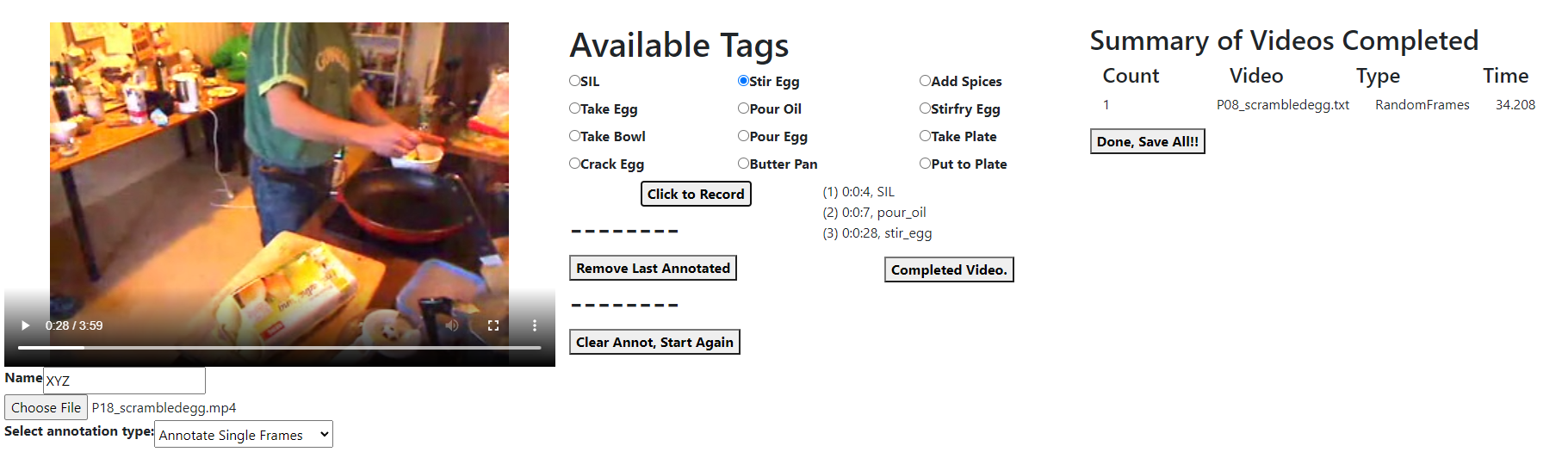
Annotation Interface: We developed a simple and user-friendly custom annotation interface to perform the user study for all three annotations, which is shown in Fig. 8. We will make the annotation tool available along with our code repository.
References
- [1] Alwassel, H., Heilbron, F.C., Escorcia, V., Ghanem, B.: Diagnosing error in temporal action detectors. In: Proceedings of the European Conference on Computer Vision (ECCV). pp. 256–272 (2018)
- [2] Carreira, J., Zisserman, A.: Quo vadis, action recognition? a new model and the kinetics dataset. In: proceedings of the IEEE Conference on Computer Vision and Pattern Recognition. pp. 6299–6308 (2017)
- [3] Chang, C.Y., Huang, D.A., Sui, Y., Fei-Fei, L., Niebles, J.C.: D3tw: Discriminative differentiable dynamic time warping for weakly supervised action alignment and segmentation. In: Proceedings of the IEEE/CVF Conference on Computer Vision and Pattern Recognition. pp. 3546–3555 (2019)
- [4] Chen, M.H., Li, B., Bao, Y., AlRegib, G., Kira, Z.: Action segmentation with joint self-supervised temporal domain adaptation. In: Proceedings of the IEEE/CVF Conference on Computer Vision and Pattern Recognition. pp. 9454–9463 (2020)
- [5] Dempster, A.P., Laird, N.M., Rubin, D.B.: Maximum likelihood from incomplete data via the em algorithm. Journal of the Royal Statistical Society. Series B (Methodological) 39(1), 1–38 (1977), http://www.jstor.org/stable/2984875
- [6] Ding, G., Yao, A.: Temporal action segmentation with high-level complex activity labels. arXiv preprint arXiv:2108.06706 (2021)
- [7] Ding, L., Xu, C.: Weakly-supervised action segmentation with iterative soft boundary assignment. In: Proceedings of the IEEE Conference on Computer Vision and Pattern Recognition. pp. 6508–6516 (2018)
- [8] Farha, Y.A., Gall, J.: Ms-tcn: Multi-stage temporal convolutional network for action segmentation. In: Proceedings of the IEEE/CVF Conference on Computer Vision and Pattern Recognition. pp. 3575–3584 (2019)
- [9] Fathi, A., Ren, X., Rehg, J.M.: Learning to recognize objects in egocentric activities. In: CVPR 2011. pp. 3281–3288. IEEE (2011)
- [10] Fayyaz, M., Gall, J.: Sct: Set constrained temporal transformer for set supervised action segmentation. In: Proceedings of the IEEE/CVF Conference on Computer Vision and Pattern Recognition (CVPR) (June 2020)
- [11] Gao, S.H., Han, Q., Li, Z.Y., Peng, P., Wang, L., Cheng, M.M.: Global2local: Efficient structure search for video action segmentation. In: Proceedings of the IEEE/CVF Conference on Computer Vision and Pattern Recognition. pp. 16805–16814 (2021)
- [12] Ishikawa, Y., Kasai, S., Aoki, Y., Kataoka, H.: Alleviating over-segmentation errors by detecting action boundaries. In: Proceedings of the IEEE/CVF Winter Conference on Applications of Computer Vision. pp. 2322–2331 (2021)
- [13] Ju, C., Zhao, P., Chen, S., Zhang, Y., Wang, Y., Tian, Q.: Divide and conquer for single-frame temporal action localization. In: Proceedings of the IEEE/CVF International Conference on Computer Vision. pp. 13455–13464 (2021)
- [14] Kingma, D.P., Ba, J.: Adam: A method for stochastic optimization. arXiv:1412.6980 (2014)
- [15] Kuehne, H., Arslan, A., Serre, T.: The language of actions: Recovering the syntax and semantics of goal-directed human activities. In: Proceedings of the IEEE conference on computer vision and pattern recognition. pp. 780–787 (2014)
- [16] Kuehne, H., Richard, A., Gall, J.: A hybrid rnn-hmm approach for weakly supervised temporal action segmentation. IEEE transactions on pattern analysis and machine intelligence 42(4), 765–779 (2018)
- [17] Kukleva, A., Kuehne, H., Sener, F., Gall, J.: Unsupervised learning of action classes with continuous temporal embedding. In: Proceedings of the IEEE/CVF Conference on Computer Vision and Pattern Recognition. pp. 12066–12074 (2019)
- [18] Lea, C., Flynn, M.D., Vidal, R., Reiter, A., Hager, G.D.: Temporal convolutional networks for action segmentation and detection. In: proceedings of the IEEE Conference on Computer Vision and Pattern Recognition. pp. 156–165 (2017)
- [19] Li, J., Lei, P., Todorovic, S.: Weakly supervised energy-based learning for action segmentation. In: Proceedings of the IEEE/CVF International Conference on Computer Vision. pp. 6243–6251 (2019)
- [20] Li, J., Todorovic, S.: Set-constrained viterbi for set-supervised action segmentation. In: Proceedings of the IEEE/CVF Conference on Computer Vision and Pattern Recognition (CVPR) (June 2020)
- [21] Li, S.J., AbuFarha, Y., Liu, Y., Cheng, M.M., Gall, J.: Ms-tcn++: Multi-stage temporal convolutional network for action segmentation. IEEE Transactions on Pattern Analysis and Machine Intelligence (2020)
- [22] Li, Z., Abu Farha, Y., Gall, J.: Temporal action segmentation from timestamp supervision. In: Proceedings of the IEEE/CVF Conference on Computer Vision and Pattern Recognition. pp. 8365–8374 (2021)
- [23] Ma, F., Zhu, L., Yang, Y., Zha, S., Kundu, G., Feiszli, M., Shou, Z.: Sf-net: Single-frame supervision for temporal action localization. In: European conference on computer vision. pp. 420–437. Springer (2020)
- [24] Moltisanti, D., Fidler, S., Damen, D.: Action recognition from single timestamp supervision in untrimmed videos. In: Proceedings of the IEEE/CVF Conference on Computer Vision and Pattern Recognition. pp. 9915–9924 (2019)
- [25] Moltisanti, D., Wray, M., Mayol-Cuevas, W., Damen, D.: Trespassing the boundaries: Labeling temporal bounds for object interactions in egocentric video. In: Proceedings of the IEEE International Conference on Computer Vision. pp. 2886–2894 (2017)
- [26] Rashid, M., Kjellstrom, H., Lee, Y.J.: Action graphs: Weakly-supervised action localization with graph convolution networks. In: Proceedings of the IEEE/CVF Winter Conference on Applications of Computer Vision (WACV) (March 2020)
- [27] Richard, A., Gall, J.: Temporal action detection using a statistical language model. In: Proceedings of the IEEE Conference on Computer Vision and Pattern Recognition. pp. 3131–3140 (2016)
- [28] Richard, A., Kuehne, H., Gall, J.: Action sets: Weakly supervised action segmentation without ordering constraints. In: Proceedings of the IEEE conference on Computer Vision and Pattern Recognition. pp. 5987–5996 (2018)
- [29] Richard, A., Kuehne, H., Iqbal, A., Gall, J.: Neuralnetwork-viterbi: A framework for weakly supervised video learning. In: Proceedings of the IEEE Conference on Computer Vision and Pattern Recognition. pp. 7386–7395 (2018)
- [30] Sener, F., Singhania, D., Yao, A.: Temporal aggregate representations for long-range video understanding. In: European Conference on Computer Vision. pp. 154–171. Springer (2020)
- [31] Sener, F., Yao, A.: Unsupervised learning and segmentation of complex activities from video. In: Proceedings of the IEEE Conference on Computer Vision and Pattern Recognition. pp. 8368–8376 (2018)
- [32] Simonyan, K., Zisserman, A.: Two-stream convolutional networks for action recognition in videos. In: Advances in neural information processing systems. pp. 568–576 (2014)
- [33] Singh, B., Marks, T.K., Jones, M., Tuzel, O., Shao, M.: A multi-stream bi-directional recurrent neural network for fine-grained action detection. pp. 1961–1970 (2016)
- [34] Singhania, D., Rahaman, R., Yao, A.: Coarse to fine multi-resolution temporal convolutional network. arXiv preprint arXiv:2105.10859 (2021)
- [35] Souri, Y., Fayyaz, M., Minciullo, L., Francesca, G., Gall, J.: Fast weakly supervised action segmentation using mutual consistency. IEEE Transactions on Pattern Analysis and Machine Intelligence (2021)
- [36] Stein, S., McKenna, S.J.: Combining embedded accelerometers with computer vision for recognizing food preparation activities. In: Proceedings of the 2013 ACM international joint conference on Pervasive and ubiquitous computing. pp. 729–738. ACM (2013)
- [37] VidalMata, R.G., Scheirer, W.J., Kukleva, A., Cox, D., Kuehne, H.: Joint visual-temporal embedding for unsupervised learning of actions in untrimmed sequences. In: Proceedings of the IEEE/CVF Winter Conference on Applications of Computer Vision. pp. 1238–1247 (2021)
- [38] Wang, D., Yuan, Y., Wang, Q.: Gated forward refinement network for action segmentation. Neurocomputing 407, 63–71 (2020)
- [39] Wang, Z., Gao, Z., Wang, L., Li, Z., Wu, G.: Boundary-aware cascade networks for temporal action segmentation. In: European Conference on Computer Vision. pp. 34–51. Springer (2020)