Embedded Point Iteration Based Recursive Algorithm for Online Identification of Nonlinear Regression ModelsThanks: G.-Y. Chen & M. Gan are with the College of Computer and Data Science, Fuzhou University, Fuzhou 350116, China (e-mail: cgykeda@mail.ustc.edu.cn; aganmin@aliyun.com).Thanks: J. Chen is with School of Science, Jiangnan University, Wuxi, 214122, China (e-mail: chenjing1981929@126.com)Thanks: L. Chen is with the Faculty of Science and Technology, University of Macau, Macau 99999, China (e-mail: longchen@umac.mo)
Abstract
This paper presents a novel online identification algorithm for nonlinear regression models. The online identification problem is challenging due to the presence of nonlinear structure in the models. Previous works usually ignore the special structure of nonlinear regression models, in which the parameters can be partitioned into a linear part and a nonlinear part. In this paper, we develop an efficient recursive algorithm for nonlinear regression models based on analyzing the equivalent form of variable projection (VP) algorithm. By introducing the embedded point iteration (EPI) step, the proposed recursive algorithm can properly exploit the coupling relationship of linear parameters and nonlinear parameters. In addition, we theoretically prove that the proposed algorithm is mean-square bounded. Numerical experiments on synthetic data and real-world time series verify the high efficiency and robustness of the proposed algorithm.
Index Terms:
Nonlinear regression models, online identification, parameter estimation, variable projection.I Introduction
Time series analysis plays a vital important role in scientific research and engineering applications. At early stage, the linear models were used as convenient tools for time series modeling and forecasting, however, they usually fail in capturing some important nonlinear behaviors presented in the time series, e.g., time irreversibility, asymmetry, and self-sustained stochastic cyclical behavior. Aware of these, researchers focused on the nonlinear models and proposed various models in different fields. For example, Ozaki & Oda [1] used the exponential autoregressive (Exp-AR) model to model the ship rolling data. In [2], Priestly constructed a general class of nonlinear models, named state-dependent autoregressive (SD-AR) model, to forecast and indicate specific types of nonlinear behavior. With simple topological structure and strong learning capability, the radial basis function (RBF) neural network offers a viable alternative to the traditional models. Vesin [3] and Shi et al. [4] adopted an RBF approach to SD-AR modeling and developed the RBF-AR model. Peng et al. [5] further extended the idea of RBF-AR to the systems that have several external inputs, and proposed the RBF-ARX model.
Most of these models mentioned above fall into a class of nonlinear regression models that take the form:
| (1) |
where , are the parameters to be estimated, is the state vector that may consist of the input or output, or any other explanatory variables in the system, and is a differentiable nonlinear function.
For offline identification, various approaches presented in the literature can be used for the parameter estimation of the nonlinear regression models, e.g., the joint optimization algorithm [6], alternating optimization method [6, 7], variable projection (VP) algorithm [8, 9], inner point solver [10], and structured nonlinear parameter optimization method (SNPOM) [11]. The VP algorithm, which takes advantage of the separable structure of nonlinear regression models, is more powerful and usually yields a better-conditioned problem [12, 13]. Empirical evidences [14, 15, 16, 17] have proven that the VP algorithm achieves faster convergence rate and is less sensitive to the initial value of the chosen parameters.
But in real applications, the data samples usually arrive sequentially, or the system is time-varying. The VP algorithm for batch data in offline scenario could not be applied to the online system. Most of the recursive algorithms presented in the literature [18, 19, 20, 21] ignore the special structure of nonlinear regression models. For example, Ngia & Sjoberg [18] treated all the parameters of the neural networks the same and proposed the recursive Gauss-Newton (RGN) and Levenberg-Marquardt (RLM) algorithms for the online learning. Asivadam et al. [19] presented a hybrid recursive Levenberg-Marquardt for feedforward neural networks, which is a strategy that optimizes linear and nonlinear parameters alternately.
Recently, Gan et al. [22, 23] incorporated the VP step into the online identification algorithm for separable nonlinear optimization problems. However, they did not properly resolve the coupling relationship between linear parameters and nonlinear parameters. In [22], the authors just used a few data samples to estimate the nonlinear parameters, and then in the subsequent learning process, only the linear parameters are updated. In [23], the VP step was introduced to update the nonlinear parameters, but the authors employed the least-squares method to eliminate the linear parameters only using the previous data samples (from time to ). This approach has two main defects: 1) If is small, the linear parameter is only determined by a small number of observations, which greatly limits the identification accuracy of the algorithm; 2) if is large, calculating generalized inverse consumes much computational cost. Both problems are contrary to the design principle of online learning algorithm.
For online learning, the most difficult problem in applying the VP strategy is how to solve the coupling relationship between the linear and nonlinear parameters in the recursive process. This motivates us to break through the framework of classic VP algorithm proposed by Golub & Pereyra [8], and explore new ideas for designing online VP algorithm. The main contribution of this paper is to analyze VP algorithm from another perspective and then to employ its equivalent form—the embedded point iteration (EPI) algorithm to design a recursive learning algorithm for online learning of the nonlinear regression models. The proposed recursive algorithm considers the coupling relationship of the linear parameters and nonlinear parameters during the recursive process. In addition, we theoretically prove that the proposed recursive algorithm is mean-square bounded. It is conceivable that the proposed recursive algorithm will be of great important because of the widespread of nonlinear regression models in the real-world applications.
The paper proceeds as follows. The equivalent form of VP algorithm is analyzed in Section II. In Section III, we introduce the recursive Gauss-Newton (RGN) algorithm for online learning of nonlinear regression models. The proposed recursive algorithm based on the EPI method is given in Section IV. Numerical experiments are carried out to confirm the performance of the proposed recursive algorithm in Section V. Finally, we draw the conclusion of this paper.
II Equivalent form of VP algorithm
In this paper, we consider the nonlinear regression model (1). Given observations , the parameter identification of model (1) can be formulized as the minimization problem
| (2) |
which can be written in a matrix form
| (3) |
where is the observation vector, the variables and are regarded as linear/nonlinear parameters, and . Golub & Pereyra [8] referred the data fitting problem with model (1) as separable nonlinear least squares (SNLLS) problems. Taking advantage of the special structure of SNLLS problems, they proposed an efficient VP strategy, which considers the coupling relationships of the linear parameters and nonlinear parameters. The basic idea of VP algorithm is to eliminate the linear parameters, and then to minimize the reduced function that only contains the nonlinear parameters.
For fixed parameter , the optimization problem (3) is convex. The optimal solution of linear parameters can be obtained by solving the linear least squares problem:
| (4) |
where is the Moore-Penrose inverse of . Replacing in (3) with (4) yields a reduced function:
| (5) |
where is a project operator. Compared with the problem (3), the reduced objective function is more complicated, although it contains fewer parameters to be estimated. Fortunately, Golub & Pereyra [8] proved that the original problem and the reduced problem achieve the same global minimizer and obtained the Jacobian matrix of the reduced function
| (6) |
where represents the Fréchet derivative of , and is generalized inverse of , which satisfies and . In [24], Kaufman proposed a simplified Jacobian matrix, which drops the second term in (6)
| (7) |
Empirical evidence [25, 9, 16] suggests that Kaufman’s simplified VP algorithm has similar performance to the full form. The complexity of the reduced function (5) and Jacobian matrices make it difficult to apply the classical VP algorithm to the online identification of nonlinear regression models directly. To overcome this difficulty, we examine the VP algorithm from another perspective in the following part.
Denote , , and as the residual of the minimization problem (3). The update direction can be derived by solving
| (8) |
Applying the linear least squares method to (8), we have
| (9) |
The method of calculating the update direction by solving (9) is referred to as the joint optimization algorithm. For fixed parameters , the optimal value of is the solution of linear least squares problem (4), which yields . Inserting it into (9), we have
| (10) |
This algorithm is named as embedded point iteration (EPI), which has been employed in bundle adjustment [26]. The equation (10) yields
| (11) |
that is,
| (12) |
The second equation holds since , . The Jacobian matrix of reduced function (5) can be calculated as
| (13) |
Replacing in (13) with (12) yields an approximated Jacobian matrix
| (14) |
which is the same as Kaufman’s form (7). Thus, the EPI approach is equivalent to the Kaufman’s VP algorithm. It is of great significance to expand the VP strategy to online systems.
III Recursive Gauss-Newton algorithm
The RGN algorithm [20] and RLM algorithm [18] are effective second-order methods for online identification of nonlinear regression models. In this section, we introduce the RGN algorithm that is useful for designing the proposed recursive method.
Denote as the parameters to be estimated in the problem (3), the cost function at time (denoted as ) can be written as follows
| (15) |
where ; and are the estimated values of nonlinear parameters and linear parameters at time , respectively. We consider the Taylor expansion of at
| (16) |
where is the infinitesimal of . Using the GN method to minimize yields
| (17) |
Specifically, the gradient and Hessian matrix of can be expressed as
| (18) |
| (19) |
where . As discussed in [18], we drop the small term to obtain an approximated Hessian matrix
| (20) |
Denote as the approximated Hessian matrix of , and as the covariance matrix of the estimated parameters . Then,
| (21) |
and the RGN formula can be expressed as
| (22) |
| (23) |
where . Note that the RGN algorithm does not take advantage of the special structure.
IV EPI based online learning algorithm
By considering the tight coupling relationship between the linear parameters and nonlinear parameters, the VP algorithm achieves excellent performance in many applications. However the complexity of the reduced function (5) and the corresponding Jacobian matrix (6) prevents the classical VP algorithm directly in real-time or time-varying systems. The equivalent form presented in Section II provides a valuable eye to design an online learning algorithm.
IV-A Algorithm
In this subsection, we propose a novel recursive algorithm (named as REPI) based on the equivalent relationship of VP algorithm and the RGN algorithm. The proposed algorithm mainly consists of three steps.
IV-A1 Eliminate the linear parameters
Instead of calculating the generalized inverse of a matrix, we employ the RLS method to estimate the linear parameters and to project them out of the objective function. Assume that are the estimated parameters using the previous observed data. For the new observation and the innovation vector , the procedure of estimating (or “eliminating”) the linear parameters can be listed as follows:
| (24) |
| (25) |
where is the corresponding covariance matrix of linear parameters .
IV-A2 Update the nonlinear parameters according to the underlying principle of EPI
The gradient of with respect to the parameters is
| (26) |
| (27) |
According to (22) and (23), the RGN algorithm utilizes the gradient to optimize the parameters. In such case, the coupling relationship between the linear parameters and nonlinear parameters is ignored.
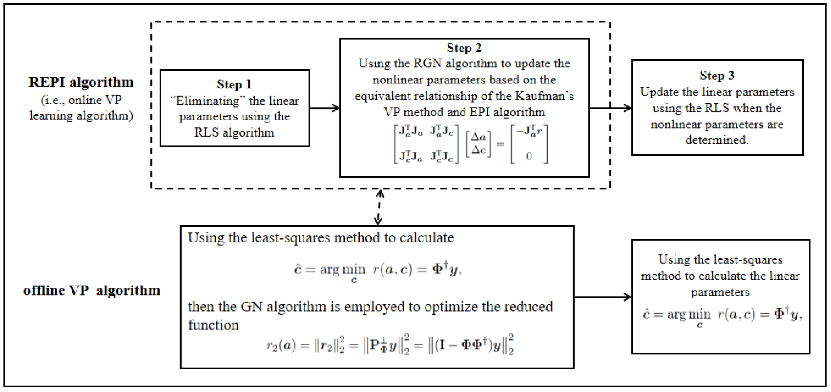
Motivated by the equivalence relationship of VP algorithm and EPI algorithm, we adopt EPI principle to update the nonlinear parameters, which considers the relationship between linear parameters and nonlinear parameters. According to (10), the derivation of the residual function with respect to linear parameters is equal to 0. With the linear parameters calculated in step 1), the gradient with respect to nonlinear parameters in (26) can be extended to
| (28) |
It can be seen from (9) and (10) that, except for the difference on the right side of the update equations, the implementation of the RGN algorithm and EPI algorithm are the same. Using the underlying principle of EPI algorithm, plugging the extended gradient (28) into (22) yields the update procedure of nonlinear parameters:
| (29) |
| (30) |
where , is the covariance matrix of estimated parameters. Unlike the RGN method, the update direction of the linear parameters included in is bypassed in this step, and it is updated using RLS method in the next step.
IV-A3 Update the linear parameters
The linear parameters are updated using the RLS algorithm after the nonlinear parameters are determined at time . Using the observation and the newest innovation vector , the linear parameters are updated as follows:
| (31) |
| (32) |
| (33) |
Remark: The idea of introducing step 1) is based on the underlying idea of the offline VP algorithm that projects out the linear parameters, resulting in a reduced function. When updating the nonlinear parameters, the proposed REPI algorithm considers the coupling relationship between the linear parameters and nonlinear parameters according to the equivalent form of the VP algorithm (presented in Section II). Fig.1 outlines the comparison of the REPI algorithm and offline VP method.
IV-B Convergence of the proposed REPI algorithm
In this subsection, we give the convergence analysis of the proposed recursive algorithm. Assume that the covariance of the linear and nonlinear parameters are bounded, that is, there exist positive constants , ,
The following two theorems indicate that the estimation error obtained by the proposed algorithm is mean-square bounded.
Definition 1. An information vector is persistently exciting [27], if there exist positive constants , , and integer number such that
For convenience, we give some instruction of some variables appearing in the theorems. and are assumed to be the true values of the parameters in the nonlinear regression models. is the gradient of residual function with respect to the parameters , and is the extended gradient that is calculated according to (28).
Theorem 1
Assume that is persistently exciting, and are martingale difference sequences [23, 27], where is the observation noise, , and is a -algebra that is generated from the observation data up to time . If and satisfy
- 1.
a.s.
- 2.
a.s.
then the estimation error of the nonlinear parameters obtained by the proposed recursive algorithm is mean-square bounded, i.e., .
Proof:
By the update equation (29), the estimation error can be expressed as
| (34) |
Let
| (35) |
and replace with (34), we have
According to (21), the recurrence of Hessian matrix is , then
| (36) | |||
Since is persistently exciting, there exist , and an integer () such that
Therefore,
then . According to the bounded assumption of , we have
Taking the conditional expectation of both side of (IV-B) with respect to , and using the conditions 1) and 2), we have
Since and are martingale difference sequences, we have is martingale sequences [23, 27]. By the martingale convergence theorem [28], converges to a finite random variable almost surely.
Theorem 2
If the innovation vector is persistently exciting, then the estimation error of the linear parameters obtained by the proposed algorithm is mean-square bounded.
V Numerical illustration
In this section, three numerical examples, including parameter estimation of a complex exponential model and fitting real-world time series using RBF-AR(X) models, are used to verify the performance of the proposed recursive algorithm.
V-A Parameter estimation of complex exponential model
We consider the complex exponential model with three basis functions here:
| (39) | |||||
where and are the linear and nonlinear parameters to be estimated respectively. As discussed in [23], the selected true parameters are and . is the Gaussian white noise with 0 mean and standard deviation 0.2, and the variable follows the standard normal distribution. Using these parameters, we randomly generate 1000 data samples.
The structure of (39) is assumed to be known, and we use the generated (observed) data to identify the parameters of the model. Four different recursive learning algorithms, including the proposed algorithm, RGN algorithm, HRGN algorithm and RVP algorithm, are employed to estimate the parameters of model (39). The HRGN algorithm is a hybrid RGN algorithm, which divides the parameters into a linear part and nonlinear part and optimizes them alternately. The RVP algorithm was proposed in [23], which just uses the previous data points to eliminate the linear parameters. The relative errors between the estimated parameters and true parameters are used to evaluate the performances of different algorithms,
| (40) |

For fair comparison, the observations and initial values of estimated parameters are kept the same for each algorithm. Fig. 2 shows the convergence process of different algorithms, and Table I lists part of the detailed results of parameter estimation during the recursive process. From Fig. 2 and Table I, we can observe that 1) the proposed recursive algorithm requires fewer observations to converge and achieves smallest estimation error, outperforming the other three algorithms; 2) similar to the off-line algorithm, the RGN algorithm that neglects the separable structure, is difficult to converge.
To further evaluate the efficiency and robustness of the proposed algorithm, we randomly generate 300 sets of initial values of the estimated parameters and observations. The generated initial values obey the uniform distribution, i.e.,
where represents a uniform distribution over the interval .

For each run, different algorithms start from the same initial points and the observations are kept the same. Fig. 3 shows the boxplot of parameter estimation errors of different recursive algorithms for 300 runs. As shown in Fig. 3, we can observe that the proposed algorithm achieves the smallest average estimation error and smallest standard derivation. Both the HRGN algorithm and RVP algorithm have some large estimation errors. This mainly because that the HRGN algorithm regards linear parameters and nonlinear parameters as independent and the RVP algorithm only uses a small amount of data (here ) to eliminate the linear parameters, which makes them sensitive to the initial values of estimated parameters.
The above comparison indicates that by introducing the EPI step, the proposed recursive algorithm is more robust and efficient than the algorithms that neglect the separable structure and the algorithms that regard the linear/nonlinear parameters as independent.
| RGN | 100 | 3.36 | 1.59 | 1.71 | 1.61 | 2.418 | 1.724 | 0.74 | 47.55 |
|---|---|---|---|---|---|---|---|---|---|
| 200 | 3.36 | 1.69 | 1.62 | 1.42 | 2.316 | 1.724 | 0.61 | 45.59 | |
| 500 | 3.27 | 1.81 | 1.62 | 1.29 | 2.140 | 1.913 | 0.49 | 40.64 | |
| 1000 | 3.24 | 1.87 | 1.63 | 1.17 | 2.050 | 1.993 | 0.44 | 38.42 | |
| HRGN | 100 | 2.59 | 1.49 | 1.60 | 2.11 | 2.49 | 2.65 | 2.93 | 56.81 |
| 200 | 2.86 | 2.26 | 1.47 | 1.74 | 1.89 | 2.56 | 2.68 | 44.71 | |
| 500 | 2.55 | 2.60 | 1.74 | 1.34 | 1.67 | 2.60 | 1.30 | 18.96 | |
| 1000 | 2.36 | 2.77 | 1.86 | 1.15 | 1.61 | 2.68 | 0.81 | 10.69 | |
| RVP | 100 | 1.63 | 3.57 | 2.01 | 1.38 | 1.36 | 3.71 | 1.35 | 21.91 |
| 200 | 1.59 | 3.52 | 1.95 | 1.24 | 1.38 | 3.66 | 1.18 | 19.04 | |
| 500 | 1.72 | 3.38 | 1.98 | 1.12 | 1.42 | 3.37 | 0.93 | 11.56 | |
| 1000 | 1.79 | 3.28 | 1.98 | 1.08 | 1.43 | 3.29 | 0.88 | 8.67 | |
| 100 | 2.20 | 3.05 | 1.81 | 1.02 | 1.58 | 3.09 | 0.63 | 6.43 | |
| proposed | 200 | 2.14 | 3.04 | 1.89 | 1.04 | 1.56 | 3.03 | 0.72 | 3.88 |
| algorithm | 500 | 2.07 | 3.00 | 1.92 | 1.02 | 1.53 | 3.01 | 0.76 | 2.18 |
| 1000 | 2.06 | 2.99 | 1.93 | 1.01 | 1.51 | 3.01 | 0.78 | 1.79 | |
| True value | 2.00 | 3.00 | 2.00 | 1.00 | 1.50 | 3.000 | 0.800 |
V-B Fitting real-world time series using RBF-AR(X) model
The RBF-AR(X) model is a powerful statistical tool for time series analysis and system modeling, which can be expressed as
where are the model order, and are the estimated parameters. The model is usually abbreviated as , when , it degenerates to a model without exogenous inputs (denoted as ). The parameter identification of RBF-AR(X) model is a typical nonlinear regression problem.
In this subsection, we use the RBF-AR(X) to model two real-world time series and assume that the data samples arrive subsequently (i.e., real-time observations). Five different recursive algorithms, including the RGN, HRLM, RVP, stochastic gradient descent (SGD) method and the proposed recursive algorithm are employed to identify the model.
V-B1 Glass tube drawing process

The process is outlined in Fig. 4, and readers can refer to [29, 30] for more details. Wall thickness is one of the most important quantities to be regulated, which is directly and easily affected by mandrel gas pressure and drawing speed. We used RBF-ARX(6,5,1,2) to characterize the dynamics of the process
where is the time delay of the process; , and represent the wall thickness, gas pressure and drawing speed, respectively; the state vector consists of the output. The data set used here (including 1269 data samples) is provided in [30]. Different algorithms are applied to identified the RBF-ARX model from the first 600 subsequently observed data samples, remaining the rest to check the predictive ability of the estimated model.
Fig. 5 shows the comparison of fitting results using the observed data samples. As shown in Fig. 5, we can observe that the proposed recursive algorithm that considers the coupling of the linear and nonlinear parameters converges quickly, requiring fewer observations. The RGN algorithm and SGD algorithm ignore the separable structure of RBF-AR model, which yields slower convergence rate and larger fitting error. The model obtained by the SGD algorithm is unstable and is easily affected by the new observations. The RVP algorithm eliminates linear parameters using least squares method, so it requires at least ( is the number of linear parameters) observations to update the parameters of the model, and the parameters are not updated at the beginning stage. The RVP algorithm just uses a few data to tackle the coupling between parameters, which leads to the instability and slow convergence of the algorithm.

| RGN | HRGN | RVP | SGD | proposed algorithm | |
| prediction accuracy | 0.5739 | 0.0269 | 0.0149 | 0.0198 | 0.0113 |
The comparison of predictive result of models identified by the different methods is listed in Table II. From Table II, we can observe that the model obtained by the REPI algorithm achieves best prediction performance among different recursive algorithms.
These results are similar to those of off-line algorithms for nonlinear regression problems [25, 9, 16, 13]. The comparison results show that similar to the off-line VP algorithm, the proposed algorithm is more suitable for the identification of nonlinear regression models by introducing the EPI step.
V-B2 Fitting thickness ozone column data
The thickness ozone column data collects 518 records of the mean thickness ozone column in Arosa, Switzerland. We do the transformation () as [31] to make it more nearly symmetric and to stabilize the variance. The transformed data are shown in Fig. 6. It is also assumed that the data arrive subsequently. We use the RBF-AR(5,1,2) to fit the data, and employ four different recursive algorithms to identify the model. The previous 300 data points are used to identify the model, remaining the rest data to check the predictive ability of estimated models.


Fig. 7 shows the convergence process of different algorithms. As shown in Fig. 7, the proposed algorithm requires fewer data samples to converge than the other four algorithms. The HRGN algorithm and RVP algorithm that take advantage of the separable structure of RBF-AR model perform better than the RGN algorithm and SGD algorithm. However, the HRGN algorithm ignores the relationship between linear parameters and nonlinear parameters and the RVP algorithm only uses a small amount of data samples to eliminate linear parameters. These limit their learning performances. The SGD algorithm converges slowly and fluctuates greatly for new observations. The detailed comparisons of prediction result of different models estimated by the five recursive algorithms are listed in Table III.
| RGN | HRGN | RVP | SGD | proposed algorithm | |
| prediction accuracy | 1.7608 | 0.1809 | 0.2235 | 2.0837 | 0.1410 |
The above comparison results indicate the high efficiency of the proposed recursive algorithm. By introducing the EPI step, the proposed algorithm can adjust the parameters of the model appropriately by handling the coupling relationship between linear parameters and nonlinear parameters.
VI Conclusion
Nonlinear regression models have been widely used in scientific research and engineering applications. The parameter identification, especially for online system, is quite challenging because of the existence of nonlinear parameters. Empirical results have proven that the VP algorithm is valuable in solving such problems. However, previous research on the VP algorithm is limited to offline problems. For online identification of nonlinear regression problems, researchers often ignore the separable structure.
In this paper, we study the recursive algorithms for nonlinear regression models and propose an efficient recursive algorithm by analyzing the equivalent form of VP algorithm. Similar to the offline VP algorithm, the proposed algorithm is more efficient and robust than the previous RGN algorithm and HRGN algorithm by introducing the EPI step. Moreover, we prove that the proposed algorithm is mean-square bounded. This study is of great important for the development of real-time systems because of the widespread of nonlinear regression models in the real-world applications.
References
- [1] T. Ozaki and H. Oda, “Non-linear time series model identification by akaike’s information criterion,” IFAC Proceedings Volumes, vol. 10, no. 12, pp. 83–91, 1977.
- [2] M. Priestley, “State-dependent models: A general approach to non-linear time series analysis,” Journal of Time Series Analysis, vol. 1, no. 1, pp. 47–71, 1980.
- [3] J.-M. Vesin, “An amplitude-dependent autoregressive model based on a radial basis functions expansion,” in 1993 IEEE International Conference on Acoustics, Speech, and Signal Processing, vol. 3. IEEE, 1993, pp. 129–132.
- [4] Z. Shi, Y. Tamura, and T. Ozaki, “Nonlinear time series modelling with the radial basis function-based state-dependent autoregressive model,” International Journal of Systems Science, vol. 30, no. 7, pp. 717–727, 1999.
- [5] H. Peng, T. Ozaki, V. Haggan-Ozaki, and Y. Toyoda, “A parameter optimization method for radial basis function type models,” IEEE Transactions on neural networks, vol. 14, no. 2, pp. 432–438, 2003.
- [6] T. Okatani and K. Deguchi, “On the wiberg algorithm for matrix factorization in the presence of missing components,” International Journal of Computer Vision, vol. 72, no. 3, pp. 329–337, 2007.
- [7] T. Okatani, T. Yoshida, and K. Deguchi, “Efficient algorithm for low-rank matrix factorization with missing components and performance comparison of latest algorithms,” in 2011 International Conference on Computer Vision. IEEE, 2011, pp. 842–849.
- [8] G. H. Golub and V. Pereyra, “The differentiation of pseudo-inverses and nonlinear least squares problems whose variables separate,” SIAM Journal on numerical analysis, vol. 10, no. 2, pp. 413–432, 1973.
- [9] G. Golub and V. Pereyra, “Separable nonlinear least squares: the variable projection method and its applications,” Inverse problems, vol. 19, no. 2, p. R1, 2003.
- [10] A. Y. Aravkin, J. V. Burke, and G. Pillonetto, “Sparse/robust estimation and kalman smoothing with nonsmooth log-concave densities: Modeling, computation, and theory,” The Journal of Machine Learning Research, vol. 14, no. 1, pp. 2689–2728, 2013.
- [11] X. Zeng, H. Peng, and F. Zhou, “A regularized snpom for stable parameter estimation of rbf-ar (x) model,” IEEE transactions on neural networks and learning systems, vol. 29, no. 4, pp. 779–791, 2017.
- [12] J. Sjoberg and M. Viberg, “Separable non-linear least-squares minimization-possible improvements for neural net fitting,” in Neural Networks for Signal Processing VII. Proceedings of the 1997 IEEE Signal Processing Society Workshop. IEEE, 1997, pp. 345–354.
- [13] G.-Y. Chen, S.-Q. Wang, M. Gan, and C. Chen, “Insights into algorithms for separable nonlinear least squares problems,” IEEE transactions on image processing, vol. 30, no. 2, pp. 1207–1218, 2021.
- [14] G.-Y. Chen, M. Gan, C. P. Chen, and H.-X. Li, “A regularized variable projection algorithm for separable nonlinear least-squares problems,” IEEE Transactions on Automatic Control, vol. 64, no. 2, pp. 526–537, 2019.
- [15] A. Y. Aravkin and T. Van Leeuwen, “Estimating nuisance parameters in inverse problems,” Inverse Problems, vol. 28, no. 11, p. 115016, 2012.
- [16] M. Gan, C. P. Chen, G.-Y. Chen, and L. Chen, “On some separated algorithms for separable nonlinear least squares problems,” IEEE Transactions on Cybernetics, vol. 48, no. 10, pp. 2866–2874, 2018.
- [17] N. B. Erichson, P. Zheng, K. Manohar, S. L. Brunton, J. N. Kutz, and A. Y. Aravkin, “Sparse principal component analysis via variable projection,” SIAM Journal on Applied Mathematics, vol. 80, no. 2, pp. 977–1002, 2020.
- [18] L. S. Ngia and J. Sjoberg, “Efficient training of neural nets for nonlinear adaptive filtering using a recursive levenberg-marquardt algorithm,” IEEE Transactions on Signal Processing, vol. 48, no. 7, pp. 1915–1927, 2000.
- [19] V. S. Asirvadam, S. F. McLoone, and G. W. Irwin, “Separable recursive training algorithms for feedforward neural networks,” in Proceedings of the 2002 International Joint Conference on Neural Networks. IJCNN’02 (Cat. No. 02CH37290), vol. 2. IEEE, 2002, pp. 1212–1217.
- [20] S. S. Shamsudin and X. Chen, “Recursive gauss-newton based training algorithm for neural network modelling of an unmanned rotorcraft dynamics,” International Journal of Intelligent Systems Technologies and Applications, vol. 13, no. 1/2, pp. 56–80, 2014.
- [21] J. Chen, Q. Zhu, and Y. Liu, “Modified kalman filtering based multi-step-length gradient iterative algorithm for arx models with random missing outputs,” Automatica, vol. 118, p. 109034, 2020.
- [22] M. Gan, X.-X. Chen, F. Ding, G.-Y. Chen, and C. P. Chen, “Adaptive rbf-ar models based on multi-innovation least squares method,” IEEE Signal Processing Letters, vol. 26, no. 8, pp. 1182–1186, 2019.
- [23] M. Gan, Y. Guan, G.-Y. Chen, and C. P. Chen, “Recursive variable projection algorithm for a class of separable nonlinear models,” IEEE Transactions on Neural Networks and Learning Systems, 2020.
- [24] L. Kaufman, “A variable projection method for solving separable nonlinear least squares problems,” BIT Numerical Mathematics, vol. 15, no. 1, pp. 49–57, 1975.
- [25] A. Ruhe and P. Å. Wedin, “Algorithms for separable nonlinear least squares problems,” SIAM review, vol. 22, no. 3, pp. 318–337, 1980.
- [26] J. Hyeong Hong, C. Zach, and A. Fitzgibbon, “Revisiting the variable projection method for separable nonlinear least squares problems,” in Proceedings of the IEEE Conference on Computer Vision and Pattern Recognition, 2017, pp. 127–135.
- [27] R. M. Johnstone, C. R. Johnson Jr, R. R. Bitmead, and B. D. Anderson, “Exponential convergence of recursive least squares with exponential forgetting factor,” Systems & Control Letters, vol. 2, no. 2, pp. 77–82, 1982.
- [28] V. Solo, “The convergence of aml,” IEEE Transactions on Automatic Control, vol. 24, no. 6, pp. 958–962, 1980.
- [29] M. Gan, H.-X. Li, and H. Peng, “A variable projection approach for efficient estimation of rbf-arx model,” IEEE Transactions on Cybernetics, vol. 45, no. 3, pp. 462–471, 2015.
- [30] Y. Zhu, Multivariable system identification for process control. Elsevier, 2001.
- [31] G.-y. Chen, M. Gan, and G.-l. Chen, “Generalized exponential autoregressive models for nonlinear time series: stationarity, estimation and applications,” Information Sciences, vol. 438, pp. 46–57, 2018.