Lens Antenna Arrays-Assisted mmWave MU-MIMO Uplink Transmission: Joint Beam Selection and Phase-Only Beamforming Design

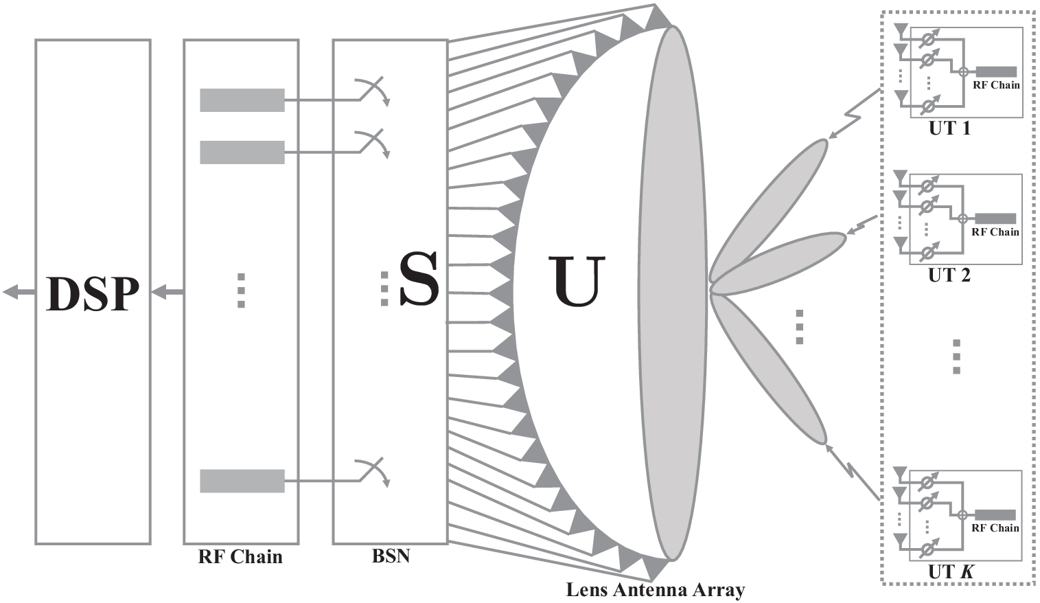
The considered mmWave MU-MIMO uplink communication system is depicted in Fig. 1, consisting of $K$ UTs and one BS. To reduce the hardware implementation costs, we assume that each UT $k\in\mathcal{K}\triangleq\left\{1,2,\ldots,K\right\}$ is equipped with a single RF chain and an $N_{k}$-element phased array to convey signals while the BS has an $N$-antenna LLA and $L$ ($K\leq L\ll N$) RF chains for receiving. We denote $\mathbf{x}_{k}\in{\mathbbmss{C}}^{N_{k}\times 1}$ as the signal vector sent by UT $k$, which satisfies $\mathbf{x}_{k}=\mathbf{w}_{k}x_{k}$ with $x_{k}\in{\mathbbmss{C}}$ and $\mathbf{w}_{k}\in{\mathbbmss{C}}^{N_{k}\times 1}$ denoting the data symbol and phase-only beamforming vector, respectively. Particularly, we have $\mathbbmss{E}\left\{x_{k}\right\}=0$, $\mathbbmss{E}\left\{x_{k}x_{k^{\prime}}^{\mathsf{H}}\right\}=0$, $\forall k\neq k^{\prime}$, and $\mathbf{w}_{k}=\frac{1}{\sqrt{N_{k}}}{\bm{\phi}}_{k}$, where ${\bm{\phi}}_{k}=\left[\phi_{k,1};\ldots;\phi_{k,N_{k}}\right]$, $\phi_{k,n_{k}}={\rm{e}}^{{\rm{j}}\theta_{{n_{k}}}}$, $n_{k}\in\left\{1,\ldots,N_{k}\right\}$, with ${\rm{j}}^{2}=-1$ and $\theta_{n_{k}}\in\left[0,2\pi\right)$ being the phase shift introduced by the $n$th element of the phased array at UT $k$. Then, the received signal at the BS is

where $\mathbf{H}_{k}\in{\mathbbmss{C}}^{N\times N_{k}}$ represents the channel matrix from UT $k$ to the BS, and $\mathbf{n}\sim{\mathcal{CN}}\left(\mathbf{0},\sigma^{2}\mathbf{I}_{N}\right)$ is the thermal noise at the BS with $\sigma^{2}$ being the noise power.

After passing through the LLA and the beam selection network (BSN), the received signal vector becomes [3, 4, 5, 6, 7, 8, 9]

where ${\mathbf{U}}\in{\mathbbmss{C}}^{N\times N}$ is a discrete Fourier transform (DFT) matrix that reflects the influence of LLA on the incident signal, and ${\mathbf{S}}=\left[S_{l,n}\right]\in{\mathbbmss{C}}^{L\times N}$ is the beam selection matrix with binary entries $S_{l,n}\in\left\{0,1\right\}$ to choose beams. It is worth noting that $S_{l,n}=1$ represents the $n$th beam is selected to connect with the $l$th RF chain. In general, each beam is selected for at most one RF chain, which yields ${\mathbf{S}}{\mathbf{S}}^{{\mathsf{H}}}={\mathbf{I}}_{L}$ [5]. Afterward, the signal vector $\mathbf{q}$ will be sent to the digital signal processor (DSP) for symbol detection as well as information decoding.

As is widely know, the sum rate capacity of an uplink MU-MIMO channel can be achieved by exploiting a minimum mean square error with successive interference cancellation (MMSE-SIC) decoder. Particularly, the uplink sum rate achieved by the MMSE-SIC decoder is given by

with $p_{k}=\mathbbmss{E}\{|x_{k}|^{2}\}$ denoting the transmit power of UT $k$.

The mmWave spatial channel can be characterized by the famous Saleh-Valenzuela (S-V) model. By assuming that the BS and all the UTs are equipped with uniform linear arrays (ULAs), the spatial channel of UT $k$ can be written as

where $M_{k}$ denotes the total number of resolvable paths, $\mu_{k}$ is the large-scale fading gain between the BS and UT $k$, $\beta_{k,l}\sim{\mathcal{CN}}\left(0,1\right)$ denotes the complex gain of the $l$th path, ${\mathbf{a}}_{T}(\psi)$ is the array response of a $T$-element ULA with $\psi$ being the angle of arrival (AoA) or angle of departure (AoD), $\varphi_{k,l}$ denotes the AoA at the BS, and $\theta_{k,l}$ denotes the AoD at UT $k$. Particularly, we have ${\mathbf{a}}_{T}(\psi)=[{\rm e}^{-{\rm j}2\pi\frac{d}{\lambda}x\sin\psi}]_{x\in{\mathcal{I}(T)}}$, where $\mathcal{I}(T)=\left\{-\frac{T-1}{2},-\frac{T+1}{2},\ldots,\frac{T-1}{2}\right\}$ is a symmetric set of indices centered around zero, $\lambda$ denotes the wavelength, and $d$ denotes the inter-antenna space. Here, we set $d=\frac{\lambda}{2}$.

In this work, we investigate the transmission strategy for the LLA-assisted MU-MIMO uplink system, where we strive to jointly optimize the transmit power, $p_{k}$, $\forall k$, as well as the phase-only beamforming vector $\mathbf{w}_{k}$, $\forall k$, at the UT sides and the beam selection matrix, $\mathbf{S}$, for improving the system performance. From a systematic perspective, we adopt the sum rate of the entire communication system as our design criterion. Then, the optimization of $p_{k}$, $\mathbf{w}_{k}$, $\forall k$, and $\mathbf{S}$ is formulated as the following problem

where ${p}\triangleq\left\{p_{k}\right\}_{k=1}^{K}$, $\mathbf{w}\triangleq\left\{{\mathbf{w}}_{k}\right\}_{k=1}^{K}$, and $p_{k,\max}$ is the maximum available transmit power at UT $k$. It is worth mentioning that the optimization problem $\mathcal{P}_{1}$ in (5) presents a different mathematical form from that defined in [11, Equ. (2)]; therefore, the proposed methods in [11] are not applicable to problem $\mathcal{P}_{1}$. It is also worth noting that problem (5) is quite challenging due to the following reasons. First, the objective function of $\mathcal{P}_{1}$ in (5a) presents a complicated form. Second, the discrete constraints in (5b) make $\mathcal{P}_{1}$ essentially an NP-hard problem. Additionally, the presence of the unit-modulus constrained ${\bm{\phi}}\triangleq\left[{\bm{\phi}}_{1}^{\mathsf{H}},\ldots,{\bm{\phi}}_{K}^{\mathsf{H}}\right]^{\mathsf{H}}\in{\mathbbmss{C}^{\sum_{k=1}^{N_{k}}\times 1}}$ further complicates the optimization procedure. In the sequel, we intend to formulate an efficient approach to address this difficult mixed-integer non-convex problem.

To proceed, we regard the sum rate in (9) as the data rate of a hypothetical communication system described by ${\mathbf{y}}_{\rm{h}}={\bm{\Delta}}\bar{\mathbf{H}}{\mathbf{s}}_{\rm h}+{\mathbf{n}}_{\rm h}$ with ${\bm{\Delta}}\bar{\mathbf{H}}$, ${\mathbf{s}}_{\rm h}\sim{\mathcal{CN}}\left({\mathbf{0}},{\mathbf{I}}_{K}\right)$, and ${\mathbf{n}}_{\rm h}\sim{\mathcal{CN}}\left({\mathbf{0}},\sigma^{2}{\mathbf{I}}_{N}\right)$ being the hypothetical channel matrix, signal symbol vector, and additive noise, respectively. Assume a matrix ${\mathbf{U}}_{\rm{h}}\in{\mathbbmss{C}}^{N\times K}$ is adopted for linear receiving, and thus the MSE matrix is given as follows

Then, by the theory of the WMMSE method [13, Theorem 1], we introduce an auxiliary optimization matrix variable ${\mathbf{W}}_{\rm{h}}\in{\mathbbmss{C}}^{K\times K}$ and apply it to establish a matrix-weighted MSE minimization problem as

Problem $\mathcal{P}_{3}$ is equivalent to problem $\mathcal{P}_{2}$ in the sense that the solutions of $\left\{{\mathbf{s}},{\bm{\phi}}\right\}$ for the two problems are identical [13, Theorem 1]. It is worth mentioning that problem $\mathcal{P}_{3}$ is more tractable than problem $\mathcal{P}_{2}$ as well as problem $\mathcal{P}_{1}$ since the objective function is convex over each variable $({\mathbf{W}}_{\rm{h}},{\mathbf{U}}_{\rm{h}},{\mathbf{s}},{\bm{\phi}})$ while holding others fixed. Furthermore, to deal with the discrete constrains (13b), we introduce the auxiliary variables $\bar{\mathbf{s}}=[\bar{s}_{1};\ldots;\bar{s}_{N}]$ subject to the constraints of ${\bar{s}}_{n}=s_{n}$, $s_{n}\left(1-{\bar{s}}_{n}\right)=0$, and $0\leq{\bar{s}}_{n}\leq 1$. Then, we can equivalently convert problem $\mathcal{P}_{3}$ as follows:

Particularly, we find that optimizing each variable of problem $\mathcal{P}_{4}$ separately while treating the others as constants leads to a series of subproblem that can be easily solved. By exploiting this property, we resort to the PDD technique to formulate a computationally efficient algorithm to tackle problem $\mathcal{P}_{4}$.

In general, the PDD-based algorithm is characterized by an embedded double loop structure [14]. Specifically, the inner loop solves the augmented Lagrangian (AL) subproblem while the outer loop aims to update the dual variables or the penalty parameter based on the constraint violation. Then, following the principle of PDD, we convert problem $\mathcal{P}_{4}$ into its AL form which is expressed as

where $\rho>0$ is the penalty parameter,

and where $\xi$, $\{\mu_{n}\}_{n=1}^{N}$, and $\{\lambda_{n}\}_{n=1}^{N}$ denote the dual variables associated with the equality constraints in (14b) and (14d). To tackle ${\mathcal{P}}_{5}$ more conveniently, we resort to the block coordinate descent method to iteratively optimize one block of variables while regarding the others as constants. To be more specific, we minimize the objective function in (15a) by sequentially updating ${\mathbf{W}}_{\rm{h}}$, ${\mathbf{U}}_{\rm{h}}$, $\bar{\mathbf{s}}$, ${\mathbf{s}}$, and ${\bm{\phi}}$ in the inner loop as follows.

In Step 1, we optimize ${\mathbf{W}}_{\rm{h}}$ by fixing the remaining variables. On this condition, ${\mathcal{P}}_{5}$ deduces to the unconstrained subproblem: ${\mathbf{W}}_{\rm{h}}^{\star}=\arg\min_{{\mathbf{W}}_{\rm{h}}}{\mathsf{tr}}\left\{{\mathbf{W}}_{\rm{h}}{\mathbf{E}}_{\rm{h}}\right\}-\log\det\left({\mathbf{W}}_{\rm{h}}\right)$. Using its first-order optimality condition, we get ${\mathbf{W}}_{\rm{h}}^{\star}={\mathbf{E}}_{\rm{h}}^{-1}$.

In Step 2, we optimize ${\mathbf{U}}_{\rm{h}}$ by fixing the remaining variables. Similar to the derivation of ${\mathbf{W}}_{\rm{h}}^{\star}$, the optimal ${\mathbf{U}}_{\rm{h}}$ is derived as ${\mathbf{U}}_{\rm{h}}^{\star}=\left(\sigma^{2}{\mathbf{I}}_{N}+{\bm{\Delta}}\bar{\mathbf{H}}{\bar{\mathbf{H}}}^{\mathsf{H}}{\bm{\Delta}}^{\mathsf{H}}\right)^{-1}{\bm{\Delta}}\bar{\mathbf{H}}$.

In Step 3, we optimize $\bar{\mathbf{s}}=[\bar{s}_{1};\ldots;\bar{s}_{N}]$ by fixing the remaining variables. The subproblem of optimizing $\{\bar{s}_{n}\}_{n=1}^{N}$ in parallel can be expressed as

where $a_{n}=1+s_{n}^{2}$ and $b_{n}=s_{n}+\rho\lambda_{n}+s_{n}^{2}+s_{n}\rho\mu_{n}$. Equation (17) features a scalar quadratic objective function and its optimal solution is given as follows:

In Step 4, we optimize ${\mathbf{s}}=[s_{1};\ldots;s_{N}]$ by fixing the remaining variables. This subproblem can be formulated as

where

with $[\mathbf{A}]_{i,j}$ denotes the $(i,j)$th element of $\mathbf{A}$, ${\bm{\lambda}}=[\lambda_{1};\ldots;\lambda_{N}]$, and ${\bm{\mu}}=[\mu_{1};\ldots;\mu_{N}]$. According to the Schur product theorem, we have $\left({\mathbf{U}}_{\rm{h}}{\mathbf{W}}_{\rm{h}}{\mathbf{U}}_{\rm{h}}^{\mathsf{H}}\right)\odot\left({\mathbf{H}}{\mathbf{H}}^{\mathsf{H}}\right)\succeq{\mathbf{0}}$ and thus ${\mathbf{G}}\succ{\mathbf{0}}$, which indicates that (19) is an unconstrained convex problem. By exploiting its first-order optimality condition, we can get ${\mathbf{s}}^{\star}=\left({\mathbf{G}}+{\mathbf{G}}^{\mathsf{T}}\right)^{-1}{\mathbf{g}}$.

In Step 5, we optimize ${\bm{\phi}}$ by fixing the remaining variables. The resultant subproblem of optimizing ${\bm{\phi}}$ is given by

where $\mathbf{b}_{\bm{\phi}}\!=\!\left[{\mathbf{b}}_{1}^{\mathsf{H}},\ldots,{\mathbf{b}}_{K}^{\mathsf{H}}\right]^{\mathsf{H}}$, $\mathbf{B}_{\bm{\phi}}\!=\!{\mathsf{BlkDiag}}\left\{{\mathbf{A}}_{1},\ldots,{\mathbf{A}}_{K}\right\}$, ${\mathbf{A}}_{k}=\frac{p_{k,\max}}{N_{k}}{\mathbf{H}}_{k}^{\mathsf{H}}{\mathbf{U}}^{\mathsf{H}}{\bm{\Delta}}^{\mathsf{H}}{\mathbf{U}}_{\rm{h}}{\mathbf{W}}_{\rm{h}}{\mathbf{U}}_{\rm{h}}^{\mathsf{H}}{\bm{\Delta}}{\mathbf{U}}{\mathbf{H}}_{k}$, and $\mathbf{b}_{k}=\sqrt{\frac{p_{k,\max}}{N_{k}}}{\mathbf{H}}_{k}^{\mathsf{H}}{\mathbf{U}}^{\mathsf{H}}{\bm{\Delta}}^{\mathsf{H}}{\mathbf{U}}_{\rm{h}}{\mathbf{W}}_{\rm{h}}\left(:,k\right)$. Here, ${\mathbf{W}}_{\rm{h}}\left(:,k\right)$ denotes the $k$th column of matrix ${\mathbf{W}}_{\rm{h}}$. The optimization of $\bm{\phi}$ in problem $\mathcal{P}_{6}$ is challenging since the unit-modulus constraints exhibit non-convexity. In the sequel, we resort to the MM technique [15] for the sake of obtaining a suboptimal solution. To proceed, it is necessary to establish an upper bound for the objective function in (21a). Based on [15], an alternative upper bound for ${\bm{\phi}}^{\mathsf{H}}\mathbf{B}_{\bm{\phi}}{\bm{\phi}}-2\Re\{{\bm{\phi}}^{\mathsf{H}}{\mathbf{b}}_{\bm{\phi}}\}$ can be established as

where ${\mathbf{L}}=\lambda_{\max}{\mathbf{I}}_{\sum_{k=1}^{K}N_{k}}$ with $\lambda_{\max}$ representing the maximum eigenvalue of matrix $\mathbf{G}$, $i$ is the iterative index, and ${\bm{\phi}}^{(i)}$ denotes the minimizer at the $(i-1)$th iteration of the MM procedure. Then, we arrive at the following surrogate subproblems as

It is worth noting that ${\bm{\phi}}^{\mathsf{H}}{\mathbf{L}}{\bm{\phi}}=\sum_{k=1}^{K}N_{k}$. By ignoring the terms independent with $\bm{\phi}$ in (23a), we can write the optimal solution to problem ${\mathcal{P}}_{\rm{mm}}^{(i)}$ as

where ${\mathsf{arg}}\left(\cdot\right)$ means the extraction of phase information. The MM-based approach proposed to handle problem (21) is summarized in Algorithm 1. Based on [15], Algorithm 1 is guaranteed to converge to a stationary point of problem (21).

After investigating the inner loop of the PDD-based method, we turn our attention to discussing its outer loop. In the outer iteration, the constraint violation is calculated as follows:

and update the dual variables by the following expressions: [14, Table I, Line 4]

where $t$ denotes the outer iteration index.

The overall PDD-based algorithm for solving problem (5) is summarized in Algorithm 2. This algorithm is guaranteed to converge to the set of stationary solutions of problem (5) [14]. After the convergence analysis of the proposed algorithm, we turn our attention to discussing its computational complexity. For clarity, let $I_{\rm{out}}$ and $I_{\rm{in}}$ denote the numbers of iterations in the outer loop and the inner loop, respectively. As previously stated, the per-iteration complexity in the outer loop is mainly originated from the BCD-based updating in the inner loop, whereas the per-iteration complexity in the inner loop is mainly composed of the complexity of updating variables $\left\{{\bm{\phi}},{\mathbf{s}},\bar{\mathbf{s}},{\mathbf{W}}_{\rm{h}},{\mathbf{U}}_{\rm{h}}\right\}$. It is clear to show that the complexity of computing the optimal results of ${\mathbf{W}}_{\rm{h}}$, ${\mathbf{U}}_{\rm{h}}$, ${\mathbf{s}}$, and $\bar{\mathbf{s}}$ is evaluated as ${\mathcal{O}}\left(K^{3}\right)$, ${\mathcal{O}}\left(N^{3}\right)$, ${\mathcal{O}}\left(N\right)$, and ${\mathcal{O}}\left(N^{3}\right)$, respectively. Moreover, the complexity of the MM-based optimization of $\bm{\phi}$ in Algorithm 1 is given by $\mathcal{O}\left(N_{\rm{U}}^{3}+I_{\rm{mm}}N_{\rm{U}}^{2}\right)$ with $N_{\rm{U}}=\sum_{k=1}^{K}N_{k}$ and $I_{\rm{mm}}$ denoting the number of iterations of Algorithm 1. Generally, we have $N>K$ and $N>N_{\rm{U}}$. Hence, the overall complexity of Algorithm 2 is estimated as ${\mathcal{O}}\left(I_{\text{out}}I_{\text{in}}\left(2N^{3}+I_{\rm{mm}}N_{\rm{U}}^{2}\right)\right)$, which is in polynomial time.

References

- [1] X. Gao et al., “Low RF-complexity technologies to enable millimeter-wave MIMO with large antenna array for 5G wireless communications,” IEEE Commun. Mag., vol. 56, no. 4, pp. 211–217, Apr. 2018.
- [2] J. Zhang, E. Björnson, M. Matthaiou, D. W. K. Ng, H. Yang and D. J. Love, “Prospective multiple antenna technologies for beyond 5G,” IEEE J. Sel. Areas Commun., vol. 38, no. 8, pp. 1637–1660, Aug. 2020.
- [3] X. Gao, L. Dai, Z. Chen, Z. Wang and Z. Zhang, “Near-optimal beam selection for beamspace mmWave massive MIMO systems,” IEEE Commun. Lett., vol. 20, no. 5, pp. 1054–1057, May 2016.
- [4] H. Tataria et al., “Uplink interference analysis with RF switching for lens-based millimeter-wave systems,” in Proc. IEEE ICC, 2018, pp. 1–7.
- [5] R. Guo et al., “Joint design of beam selection and precoding matrices for mmWave MU-MIMO systems relying on lens antenna arrays,” IEEE J. Sel. Topics Signal Process., vol. 12, no. 2, pp. 313–325, May 2018.
- [6] C. Feng, W. Shen, and J. An, “Beam selection for wideband millimeter wave MIMO relying on lens antenna arrays,” IEEE Commun. Lett., vol. 23, no. 10, pp. 1875–1878, Oct. 2019.
- [7] P. Liu et al., “Intelligent reflecting surface aided NOMA for millimeter-wave massive MIMO with lens antenna array,” IEEE Trans. Veh. Technol., vol. 70, no. 5, pp. 4419–4434, May 2021.
- [8] Z. Cheng, Z. Wei, and H. Yang, “Low-complexity joint user and beam selection for beamspace mmWave MIMO systems,” IEEE Commun. Lett., vol. 24, no. 9, pp. 2065–2069, Sep. 2020.
- [9] J. Sun et al., “Joint user grouping and beam selection for beamspace mmWave multi-user MIMO system,” IEEE Commun. Lett., vol. 26, no. 5, pp. 1170–1174, May 2022.
- [10] Z. Cheng, Z. Wei, H. Li, and H. Yang, “SLNR-based beamspace precoding and beam selection for wideband mmWave massive MIMO”, IEEE Commun. Lett., vol. 26, no. 2, pp. 478–482, Feb. 2022.
- [11] Z. Cheng, Z. Wei, C. Ouyang, and H. Yang, “Joint RF precoding and beam selection design for uplink mmWave beamspace MIMO systems,” IEEE Commun. Lett., Early Access, 2022.
- [12] A. Liu and V. K. N. Lau, “Phase only RF precoding for massive MIMO systems with limited RF chains,” IEEE Trans. Signal Process., vol. 62, no. 17, pp. 4505–4515, Sep. 2014.
- [13] Q. Shi et al., “An iteratively weighted MMSE approach to distributed sum-utility maximization for a MIMO interfering broadcast channel,” IEEE Trans. Signal Process., vol. 59, no. 9, pp. 4331–4340, Sep. 2011.
- [14] Q. Shi and M. Hong, “Penalty dual decomposition method for nonsmooth nonconvex optimization–Part I: Algorithms and convergence analysis,” IEEE Trans. Signal Process., vol. 68, pp. 4108–4122, 2020.
- [15] J. Song, P. Babu, and D. P. Palomar, “Sequence design to minimize the weighted integrated and peak sidelobe levels,” IEEE Trans. Signal Process., vol. 64, no. 8, pp. 2051–2064, Apr. 2016.
- [16] M. Gharavi-Alkhansari and A. B. Gershman, “Fast antenna subset selection in MIMO systems,” IEEE Trans. Signal Process., vol. 52, no. 2, pp. 339–347, Feb. 2004.