Natural Thresholding Algorithms for Signal Recovery with Sparsity
Abstract
The algorithms based on the technique of optimal -thresholding (OT) were recently proposed for signal recovery, and they are very different from the traditional family of hard thresholding methods. However, the computational cost for OT-based algorithms remains high at the current stage of their development. This stimulates the development of the so-called natural thresholding (NT) algorithm and its variants in this paper. The family of NT algorithms is developed through the first-order approximation of the so-called regularized optimal -thresholding model, and thus the computational cost for this family of algorithms is significantly lower than that of the OT-based algorithms. The guaranteed performance of NT-type algorithms for signal recovery from noisy measurements is shown under the restricted isometry property and concavity of the objective function of regularized optimal -thresholding model. Empirical results indicate that the NT-type algorithms are robust and very comparable to several mainstream algorithms for sparse signal recovery.
Index Terms:
Signal recovery, compressed sensing, thresholding algorithms, restricted isometry property, concave minimization, regularization methodI Introduction
Under the sparsity assumption, the problem of signal recovery from nonadaptive linear measurements can be formulated as a sparse optimization problem which may take different forms, depending on such factors as recovery environment, signal structure, and the prior information available for the signal [1, 2]. A fundamental mathematical model for sparsity-based signal recovery can be described as follows. Let be an sensing matrix with and let be the measurements for the signal , where are the measurement errors. When is -sparse or -compressible, the recovery of can be formulated as the following sparsity-constrained optimization (SCO) problem:
| (1) |
where is a given integer number reflecting the number of significant entries of the signal to recover, and denotes the number of nonzero entries of the vector In this paper, we say that is -sparse if and is -compressible if it can be approximated by a -sparse vector. The SCO problem plays a vital role in the development of algorithms for compressed-sensing-based signal recovery (see, e.g., [1, 2, 3, 4]). Essentially, the model (1) is to find the best -term approximation of the target signal, which best fits the acquired measurements. Similar models also arise in numerous areas such as statistical learning [5, 6, 7], wireless communication [8, 9], low-rank matrix recovery [10, 11, 12, 13, 14], linear inverse and optimization problems [15, 16, 17, 18].
While the SCO and related problems can be solved via convex optimization, nonconvex optimization and orthogonal matching pursuit (OMP) (see, e.g., [1, 2, 3, 4]), the thresholding methods with low computational complexity are particularly suited for solving the SCO model. Thus we focus our attention on the study of thresholding methods in this paper. The earlier thresholding methods mainly adopt the soft thresholding operator [19, 20, 21, 22]. The recent ones (e.g., [3, 23, 24, 25, 26, 27]) mainly use the hard thresholding operator, denoted by which retains the largest magnitudes of a vector and sets other entries to zeros. The latest development of thresholding methods, including acceleration, matrix form, dual thresholding and Newton-step-based modifications, can be found in such references as [7, 14, 28, 29, 30, 31, 32, 33]. However, performing hard thresholding on an incompressible iterate, generated by an iterative method, does not ensure the reduction of the objective value of (1) at every iteration. Motivated by this observation, the so-called optimal -thresholding (OT) method was first introduced in [34], which allows the vector thresholding and objective reduction to be performed simultaneously. Based on the OT concept, the relaxed optimal -thresholding (ROT) algorithm and their variants were also developed in [34]. A further analysis of these algorithms was performed in [35], and the algorithm using both OT technique and truncated gradient descent direction was studied in [37]. Compared to existing hard-thresholding algorithms, the strength of OT-type methods lies in their observed robustness for sparse signal recovery and steadiness in objective reduction in the course of iterations. However, the OT algorithm needs to solve a quadratic optimization problem at every iteration to obtain the optimal or nearly optimal -thresholding of a vector, and thus the computation is expensive especially for high-dimensional signal recovery.
This paper pursues a new algorithmic development which is significantly different from the existing ones in [34] and [35]. The main idea of the paper is to introduce an auxiliary regularized counterpart for the so-called binary OT model, which will be defined by (3) later in this paper. Based on such a regularized model, we utilize the traditional linearization technique (i.e., the first-order approximation method) to develop a new framework of algorithms which admits a low computational cost at every iteration, compared to general convex optimization methods. The thresholding technique adopted in this framework is referred to as the natural thresholding (NT). Such thresholding is determined by the smallest entries of the gradient of the so-called regularized objective of OT or ROT model which will be recalled in the next section. The NT algorithm takes the advantage of the ‘nice structure’ of the polytope with -sparse binary extreme points. The main work of the paper includes:
- (i)
Develop a novel class of NT-type methods for signal recovery;
- (ii)
Rigorously prove the guaranteed performance of NT-type algorithms under some conditions.
We also carry out experiments on random problem instances to show that the NT-type algorithms are fast algorithms, and their performances are very comparable to several mainstream compressed sensing algorithms.
The paper is structured as follows. The NT-type algorithms are proposed in Section II. The theoretical analysis of the algorithms is performed in Section III, and a further discussion of regularization functions and parameters is given in Section IV. The simulation results are reported in Section V.
Notation: All vectors are column vectors unless otherwise stated. For vector and matrix , and denote their transposes. We use to denote the support of the vector , i.e., the index set of nonzero entries of We use to denote the index set of the largest magnitudes of and to denote the index set of the smallest entries of When () is not uniquely determined, i.e., when there are two magnitudes (entries) being equal, we select the smallest entry indices to avoid the ambiguity in index selection. Given we denote by the complement set and by the cardinality of Given the vector is obtained from by retaining the entries supported on and setting other entries to zeros. Throughout the paper, and denote the -norm and -norm of a vector, respectively. For vectors and is the Hadamard product (entry-wise product) of the two vectors. Also, we summarize the main acronyms of algorithms in the following table.
| Acronyms | Algorithms |
|---|---|
| IHT | Iterative hard tresholding |
| HTP | Hard tresholding pursuit |
| SP | Subspace pursuit |
| CoSaMP | Compressive sampling matching pursuit |
| OMP | Orthogonal matching pursuit |
| OT | Optimal -thresholding |
| OTP | Optimal -thresholding pursuit |
| ROTP | Relaxed optimal -thresholding pursuit |
| NT | Natural thresholding |
| NTP | Natural thresholding pursuit |
| NTq | Natural thresholding with inner iter. |
| NTPq | Natural thresholding pursuit with inner iter. |
II Natural Thresholding Algorithms
Let us first recall the iterative hard thresholding (IHT), hard thresholding pursuit (HTP) and the newly developed optimal -thresholding (OT) algorithm. These algorithms provide a basis for the development of our new algorithms called natural thresholding.
II-A Basic hard thresholding algorithms: IHT and HTP
Given , the gradient of the error metric is given by At the iterate let be the vector generated by the classic gradient descent method, i.e.,
| (2) |
where is a steplength. Using the operator to generate an iterate satisfying the constraint of the problem (1) leads to the well-known IHT algorithm [15, 25, 26] and its enhanced version HTP [27]. A good feature of IHT and HTP is that they are easier to implement than other algorithms such as convex optimization [38, 39, 40, 41], orthogonal matching pursuit (OMP) [42, 43, 44], compressive sampling matching pursuit (CoSaMP)[45], and subspace pursuit (SP) [46].
IHT algorithm. Given the problem data and initial point perform the following iteration until a stopping criterion is met: At , choose and set
where is given by (2).
HTP algorithm. Given the problem data and initial point perform the following iteration until a stopping criterion is met: At , choose and let be given by (2). Then set
Clearly, the terms of selected by are not necessarily the best terms in the sense that they might not be the terms that best fit the linear measurements. As pointed out in [34], performing the hard thresholding of is independent of the error metric Thus it may happen that the value of the error metric at the point is larger than that of the current iterate i.e., This observation motivates the recent development of optimal -thresholding algorithms in [34, 35].
II-B Optimal -thresholding algorithms
As defined in [34], the optimal -thresholding of a vector , denoted by is given by which is the Hadamard product of and where is the solution to the problem
where e is the vector of ones, and the vector is -sparse and binary with exactly entries equal to 1. Given such a binary vector the Hadamard product of and retains entries of only and sets other entries to zeros. Based on the operator the conceptual optimal -thresholding (OT) method and the optimal -thresholding pursuit (OTP) were proposed in [34]. The two methods share the same first step except for the second step at which OTP performs an orthogonal projection.
OT and OTP algorithms. Given the problem data and a starting point Perform the following steps until a stopping criterion is satisfied:
- S1
Let be given as (2) and let be the solution to the problem
(3) - S2
Generate as follows:
-
For OT algorithm,
-
For OTP algorithm, let and
We would rather treat OT and OTP as conceptual algorithms due to the fact that directly solving the binary problem (3) might be expensive when the dimension of the problem is high. A more practical way is to solve a convex relaxation of (3), which can be solved by existing interior-point methods. This consideration leads to the relaxed optimal -thresholding (ROT) and relaxed optimal -thresholding pursuit (ROTP) introduced in [34, 35].
ROT and ROTP algorithms. Given the problem data and a starting point perform the steps below until a stopping criterion is satisfied:
- S1
- S2
Set and generate as follows:
-
For ROT algorithm,
-
For ROTP algorithm, let
While the optimization problem (4) can be solved efficiently by existing convex optimization solvers, the computational cost remains high for large-scaled signal recovery problems, compared with the algorithms which involve only orthogonal projection, hard thresholding or linear programming solving. This stimulates the natural thresholding (NT) method described in the next subsection.
II-C Natural thresholding algorithms: A new framework
The model (4) is a convex relaxation of (3). However, such a relaxation might be too loose, and thus its solution is usually not binary. To overcome such a drawback of (4), we may introduce a certain regularization term into the objective of (4) so that the regularized model can approximate the model (3) appropriately and the chance for the solution of regularized model being binary is enhanced. We now describe such a regularized model which is essential for the development of new algorithms in this paper. In fact, given vector consider the model of the form:
| (5) | |||||
where is a parameter and is referred to as a binary regularization function which is formally defined as follows.
Definition II.1
is said to be a binary regularization if it satisfies the following two properties: i) is a positive and continuously differentiable function over an open neighborhood of the region ii) attains its minimum value over at any binary vector and only at such binary vectors.
Example II.2
Note that given any positive number , the function is positive and continuously differentiable over the interval which is an open neighborhood of the interval [0,1]. attains its minimum value at or and for any For simplicity, we set and only consider the specific function By using this univariate function, we may construct a binary regularization function in as follows:
| (6) |
It is evident that the function (6) satisfies the properties specified in Definition II.1. More examples of binary regularization functions will be given later in this section.
Given a vector we use and to denote the functions
| (7) |
The function is the objective of the problem (5). The parameter is referred to as the regularization parameter. The solution of (5) depends on the parameter Thus for any given we use to denote the solution of (5). can be seen as the penalty for the variable violating the 0-1 restriction. From the classic optimization theory for penalty functions (see, e.g., [47]), it is not difficult to see that as the value of will decrease to its minimum in the feasible set of (5). Such minimum attains only at 0-1 vectors according to the definition of binary regularization. This implies that tends to a 0-1 point in as and any accumulation point of must be a solution to the problem (3). We summarize this fact in the following lemma whose proof is given in Appendix A for completeness.
Lemma II.3
Let in (5) be a binary regularization and be a solution of (5). Consider any strictly increasing and positive sequence satisfying Then the sequence is nonincreasing and converges to the minimum value of over and the sequence is nondecreasing and converges to the optimal value of (3). Moreover, any accumulation point of is the optimal solution of (3).
The above lemma shows that the model (5) can approximate the model (3) to any expected level of accuracy provided that the parameter is taken large enough. From this perspective, the model (5) as an approximation of (3) is better than the convex relaxation (4). By the definition, a binary regularization is nonconvex. As shown by (6), it is very easy to construct a binary regularization which is concave. As a result, the objective function of (5) can be naturally made to be concave by properly choosing the parameter Thus for the convenience of discussion, we assume that is concave throughout the remainder of this section and Section III. The concavity of the function can be guaranteed if and are chosen properly. Note that if is twice continuously differentiable, then the Hessian of is given as
from which it can be seen that when is negative definite, then will be negative semi-definite (and thus is concave) provided that is large enough.
Take (6) as an example. It is easy to verify that the Hessian of (6) is where is the identity matrix. Thus when (6) is used, the Hessian of is given as
where Note that is negative semi-definite over the whole space provided that which can be guaranteed when is not smaller than the largest eigenvalue of the matrix i.e., Therefore, the function is always concave over provided that
Note that (3) is to find the optimal -thresholding of The above discussion indicates that performing the optimal -thresholding of a vector can be approximately achieved by solving the problem (5) which from the above discussion can be made to be a concave minimization problem which remains NP-hard in general [49, 50]. The fundamental idea of the traditional MM method for solving a nonconvex optimization problem is to replace the ‘difficult’ objective function of the problem with a certain relatively easy surrogate convex function that dominates the original objective function (see, e.g., [51, 52]). For a concave objective, the simplest surrogate function is its first-order approximation at any given point. Thus the first-order approximation of the concave function can be used to develop an algorithm with significantly low computational cost.
Specifically, suppose that is the current iterate. At by the concavity of over an open neighborhood of denoted by one has
| (8) |
for any , where denotes the gradient of at Specifically, if is given by (6), the gradient of at is given as
The relation (8) shows that the first-order approximation of dominates on the whole open set By the idea of MM methods, the problem (5), i.e., where
can be approximated by its surrogate counterpart which, in this case, is the linear programming (LP) problem
Removing constant terms in the objective above, the above LP problem is reduced to
| (9) |
Let be the solution to this problem. We may replace with and repeat the above process until a certain stopping criterion is met. This is the basic idea for the development of a new algorithm.
We now point out that there is no need to solve the LP problem (9) by an algorithm since an optimal solution of (9) can be obtained explicitly due to the nature of the polytope In fact, according to the classic LP theory, the problem (9) must have an optimal solution, denoted by which is an extreme point of the polytope As shown in [34], any extreme point of is -sparse and binary. Hence the optimal value is actually the summation of entries of the vector Clearly, the smallest value of the function over the polytope is the sum of the smallest entries of Thus the optimal solution of the LP problem (9) can be explicitly given as follows. It is determined by the support of the smallest entries of , i.e., if , otherwise, for where is the index set of the smallest entries of a vector. We now describe the algorithms which are referred to as the natural thresholding (NT) and the natural thresholding pursuit (NTP) in this paper.
Input and an initial point . Repeat the following steps until a certain stopping criterion is satisfied:
- S1
- S2
Generate according to the following procedure:
-
For NT algorithm,
-
For NTP algorithm, set and
The only difference between the two algorithms is that NT does not perform an orthogonal projection, but NTP does. At the beginning of every iteration of NT and NTP, the initial point can be any given -sparse and binary vector. In particular, we may use the binary vector (10) as an initial point determined by .
Remark II.4
which together with the concavity of implies that (This fact will be used in the proof of Lemma III.2 later.) In fact, the concavity of and (12) implies that
i.e.,
Since and are 0-1 vectors at which achieves the minimum value over Thus the above inequality reduces to This means the iterate generated by NT or NTP is never worse than the one generated by IHT or HTP from the perspective of the error metric If is not optimal to (9), then and hence Thus in this case the algorithm finds the terms of which is better than the terms selected by the hard thresholding.
The NT and NTP algorithms perform linearization of only once in every iteration. We may perform linearization more than once within their step S1, i.e., replacing the role of with and repeating the step S1 of NT more than once so that a point better than might be found. Such iterations within S1 are referred to as inner iterations. Repeating the inner iterations up to times yields the algorithms NTq and NTPq.
Input , initial point and integer number Repeat the steps below until a stopping criterion is met:
-
For NTq algorithm, set
-
For NTPq algorithm, let and
Remark II.5
NT, NTP, NTq and NTPq are referred to as the NT-type algorithms in this paper. When these algorithms become NT and NTP, respectively. If is a large number, according to linearization theory for concave minimization (e.g., [49, 53]), the inner iterations of NTq and NTPq will terminate at a stationary point of the concave minimization problem in which case If we expect such a point, we may set and use as the termination criterion for inner iterations. The corresponding algorithms can be referred to as NT∞ and NTP∞ which are omitted here.
Remark II.6
As pointed out in [35], performing one iteration of ROTP requires about flops, where is the size of the problem data encoding in binary. The complexity of NT-type algorithms is much lower than that of ROTP. In fact, at every iteration, the NT-type algorithms need to compute the vector and which require about operations, and to perform and on a vector which require about flops by a sorting approach, where The NTP and NTPq algorithms need to perform the orthogonal projection where which requires about flops (see [35] for details). Thus the complexities of NT and NTP are about and flops in every iteration, respectively. If the inner iterations are executed times, then the NTq and NTPq require about and flops.
II-D Concave regularization function
Before we analyze the guaranteed performance of NT-type algorithms, it is necessary to construct more examples of concave binary regularization functions. We still construct such functions based on the kernel univariate one which is concave and positive over an open neighborhood of the interval Assume is another concave and strictly increasing univariate function over the interval Then the composite function must be a concave function over an open neighborhood of the interval due to the fact
where the last inequality follows from the fact and We may use such a function to construct a binary regularization as follows:
| (13) |
The function constructed like this can be used in NT-type algorithms. We now give two such specific functions.
- •
Let which is concave and strictly increasing over the interval Then
(14) is a concave binary regularization over an open neighborhood of the region
- •
Let which is concave and strictly increasing over the interval Then
(15) is a concave binary regularization over an open neighborhood of the region
Similar to which is related to , the regularization can be also made related to Such a regularization will be discussed in more detail in Section IV.
III Guaranteed performance and stability
In this section, we perform a theoretical analysis for the NT-type algorithms described in previous section. This analysis is made under the assumptions of concavity of and restricted isometry property (RIP), which is initially introduced by Candès and Tao [39]. An matrix where is said to satisfy the RIP of order if where is the smallest nonnegative number such that
for any -sparse vector The number is called the restricted isometry constant (RIC) of The following property of has been widely used in the analysis of compressed sensing algorithms.
It is worth stressing that RIP is not the unique assumption under which the compressed sensing algorithms can be analyzed. Other assumptions such as the mutual coherence [1, 3], null space property [3], and range space property of [4, 54] can be also used to analyze the theoretical performance of a compressed sensing algorithm. We now prove that the iterates generated by the NT-type algorithms with a concave binary regularization can guarantee to recover the sparse signal under the RIP assumption. We begin with the following lemma.
Lemma III.2
Let be a concave function, and let be the initial point of step S1 in NTq and NTPq algorithms where and let be the final output of step S1. Then
| (16) |
Proof. The inner iterations within step S1 of NTq and NTPq start from the initial point Then the first inner iteration performs the update (11) to yield the next inner iterate As pointed out in Remark II.4, since is concave and are 0-1 vectors, one must have that Then the inner iteration starts from to generate the second iterate Again, by the same argument in Remark II.4, one has Repeating this inner process times, the final output of step S1 satisfies that
Denote by the final output of S, the above inequality immediately implies the desired relation (16).
The next lemma is very useful in our analysis.
Lemma III.3
We now prove the guaranteed performance of the NT-type algorithms under RIP and concavity of It is sufficient to show the main result in noisy settings. The result for noiseless cases can be obtained immediately as a special case of our results. The practical signal is usually not exactly -sparse. Thus we are interested in recovering the key information of the signal, i.e., the largest magnitudes of the signal. For simplicity, we only analyze the algorithms with steplength The performance of the proposed algorithms with may be established by a more complicated analysis which requires significant further investigation. In fact, for the case the term would appear in (40) in the proof of Theorem III.4 below. See Appendix B for details. Thus, to bound the term in (40), the classic Lemma III.1 cannot be used, and some new technical results involving must be established first. We leave such a possible generalization as a future research work.
Theorem III.4
Let be the acquired measurements for the signal where are measurement errors. Denote by Suppose that the RIC of satisfies
| (17) |
where is the unique real root of the univariate equation in the interval where Suppose that the sequence is generated by the algorithm NT or NTq with and being concave. Then the sequence satisfies the following relation:
| (18) |
where
| (19) |
and is a constant given by
| (20) |
which is smaller than 1 under the condition (17).
The proof of Theorem III.4 is given in Appendix B. It should be pointed out that to ensure the concavity of , one may use concave binary regularization and choose to be large enough (see Section IV for more discussions). The only difference between NTq and NTPq is that the latter uses the orthogonal projection to generate from The following property of orthogonal projection is widely used in the analysis of compressed sensing algorithms.
Lemma III.5
Theorem III.6
Let be the measurements of the signal with measurement errors If the RIC of satisfies
| (21) |
then the sequence generated by the algorithm NTP or NTPq with and being concave, satisfies the following relation:
| (22) |
where is a constant given by which is smaller than 1 under (21), and are the constants given by
| (23) |
in which are the constants given in Theorem III.4.
Proof. By the structure of NTP and NTP is the output of S1, and is -sparse. The iterate is the solution to the orthogonal projection
Let By treating and as well as , it follows from Lemma III.5 that
The intermediate point generated at the th iteration of NTP (NTPq) are exactly the iterate generated at the th iteration of NT (NTq). By Theorem III.4, we have
where , are given in Theorem III.4. Combining the above two relations, we immediate obtain that
where
and
Since one has Thus is guaranteed if which is ensured under the condition Thus the bound (22) is valid.
When the measurements are accurate and the signal is -sparse, we immediately have following corollary.
Corollary III.7
Suppose that the signal is -sparse and Then the following two statements are valid:
(i) If the RIC of satisfies (17), then the sequence generated by NT or NTq with and concave converges to
(ii) If the RIC of satisfies (21), then the sequence generated by NTP or NTPq with and concave converges to
The main results established in this section indicate that the significant information of the signal can be recovered by the NT-type algorithms under RIP and concavity of Corollary III.7 further claims that under the same conditions, the -sparse signal can be exactly recovered when the measurements are accurate.
The above results also imply that the NT-type algorithms are stable for signal recovery. To establish such a stability result, let us first state the next lemma which follows immediately from Lemma 6.23 in [3].
Lemma III.8
[3] Let be an even number. Suppose that has the restricted isometry constant Given and if two vectors satisfy that and where then one has
where
In fact, by setting and considering the -norm bound, Lemma 6.23 in [3] immediately reduces to the above lemma. The following stability result for NT-type algorithms follows from Theorems III.4, III.6 and Lemma III.8.
Theorem III.9
Let be the measurements of the signal where are the measurement errors. Then the following two statements are valid:
Proof. (i) Under (17), Theorem III.4 claims that the sequence generated by NT and NTq with and concave satisfies (18). Note that where is the largest singular value of Thus (18) implies that
where and and hence
where the last inequality follows from the fact and By Lemma III.8 with and and , we immediately obtain the bound (24).
IV Further discussion on regularization and parameter
Clearly, the choice of regularization and parameter will directly affect the numerical behavior of the algorithm. The NT-type algorithms are developed from the first-order approximation of the function To ensure the quality of such an approximation, the gap between and its first-order approximation over the set should be made as small as possible. Thus we should choose and such that the second-order term in the Taylor expansion of can be dominated as possible by its first-order term. One of the ideas is to strengthen the first-order approximation by suppressing the second-order term through controlling the eigenvalues of the Hessian matrix of . This might be partially achieved by properly selecting Moreover, the concavity of can also be maintained by the proper selection of as shown by the next proposition.
Proposition IV.1
(i) Using the function (6), is concave for any given
(ii) Using the function (14), is concave for any given parameter
(iii) Using the function (15), is concave for any given parameter
The proof of the proposition is given in Appendix C. Note that the functions (6), (14) and (15) are independent of It should be pointed out that all regularization functions given in Section II can also be modified to include the vector For instance, the function (6) can be modified to involve the vector as follows:
| (26) |
where When for , this function is positive over an open neighborhood of and it remains a binary regularization specified by Definition II.1. We also have the following observation.
Proposition IV.2
When all entries of are nonzero, if is given by (IV), then is concave over an open neighborhood of for any given
Proof. The Hessian of is given as
The result is obvious since if and only if
While the concavity of is assumed for the analysis of algorithms in Section III, this assumption is largely for the convenience of analysis and might not necessarily be needed if we adopt another way of analysis. In fact, the key idea behind the derivation of the NT algorithms is the first-order approximation of the function . Such a derivation may not require the concavity of Even if is not concave, the first-order approximation of still yields the same version of the NT-type algorithms. Also, the concavity of may not be required from a numerical point of view. The value of may be simply prescribed beforehand or be updated in the course of iterations according to some rule.
The NT-type algorithms only involve the product between matrices and vectors, sorting and orthogonal projections, and hence the computational cost is very similar to that of HTP, SP, CoSaMP and OMP. The computational cost of these algorithms is much lower than convex optimization methods [38, 39, 40, 41] and optimal -thresholding methods [34, 35]. The empirical results in next section indicate that by approximate choices of the steplength and parameter the NT-type algorithms can efficiently reconstruct sparse signals.
V Numerical Validation
Based on random problem instances of signal recovery, we provide some preliminary experiment results to demonstrate the performance of the NT-type algorithms. For the given size and class of random matrices, we first use simulations to find suitable steplength and parameter for the algorithms. Then we compare the performance of NT-type algorithms and SP, CoSaMP, OMP and HTP. The dimension of the synthetic sparse signal is 8000, and the size of random matrices used in our experiments is All matrices are Gaussian matrices with columns being normalized, whose entries are independently and identically distributed (iid) random variables following the standard normal distribution. The nonzeros of sparse signals are also assumed to be iid random variables following the standard normal distribution, and their positions are uniformly distributed. Unless otherwise specified, we use the following stopping criterion for signal recovery:
| (27) |
where denotes the target signal to recover and denotes the iterate produced by an algorithm. When satisfies (27), the recovery of is counted as success, otherwise unsuccess. All results demonstrated in this section are obtained by using the function (IV) and adopting the initial point for algorithms. The maximum number of iterations for iterative algorithms is set to be 150. If an algorithm cannot meet the stopping criterion (27) in 150 iterations, the algorithm is then treated as unsuccess for the underlying recovery problem. Since NTP and NTPq use the orthogonal projection at every step, they usually outperform NT and NTq in signal recovery. Thus we only demonstrate the performance of NTP and NTPq in this section.
V-A Choice of regularization parameter:
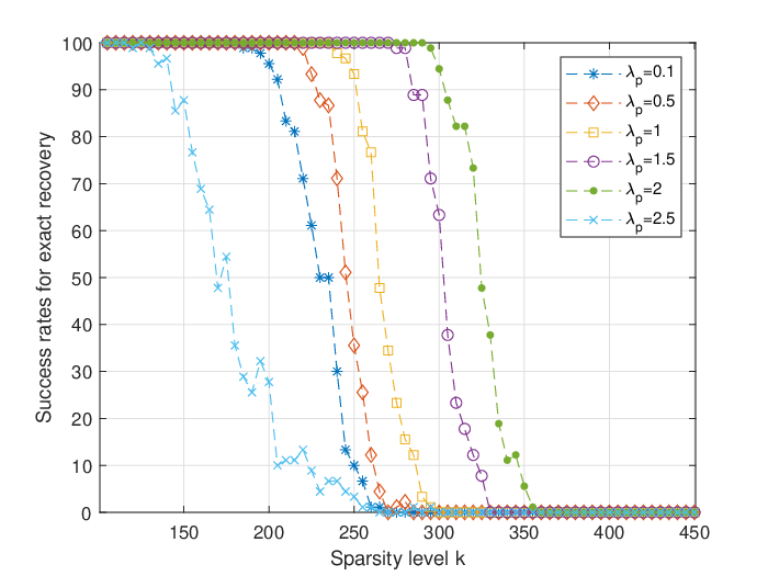
The parameter in NT-type algorithms can take any value in To see how the value of affects the performance of the algorithms, we compare the success frequencies of the algorithms for signal recovery with several different values of The sparsity of signals are ranging from 100 to 450 with stepsize 5, and the measurements are taken as for every realized random pair Our initial simulations indicate that the number of inner iterations of NTPq does not remarkably affect its overall performance. Thus we mainly consider the algorithm with i.e., the NTP algorithm, in this experiments. For each given sparsity level , 100 random trials are used to estimate the success rates of the NTP, and the algorithm is performed up to a total of 150 iterations. Fig. 1 shows the results for NTP with several different values of The steplength is fixed as (this stepsize is suggested from simulations. See the next subsection for details). The results in Fig.1 indicates that for the Gaussian matrices of size is a reasonable choice for NTP. However, we should keep in mind that such a choice of the parameter depending on the size/class of problem instances should not be generalized to other size/class of the problems.

V-B Influence of iterative steplength:
In traditional function minimization scenarios, receding in the direction of negative gradient of a function from the current iterate by a small steplength can guarantee the descent of the function. Thus the steplength in traditional optimization method is usually smaller than 1. However, when solving the SCO problem (1), this property of steplength is lost since the main purpose of the iterative algorithm for SCO is to identify the correct support of the solution instead of seeking immediate descent of the objective value. Thus when solving the SCO, the steplength of an iterative algorithm may not necessarily be smaller than 1. Indeed, a large amount of simulations indicate that the efficient steplength longer than 1 is commonly observed when solving a SCO problem. For Gaussian sensing matrices, we carried out experiments to show how the steplength might affect the performance of NTP. The random pair of are generated exactly as in previous subsection, and we set for NTP in our experiments. For every given sparsity level and steplength, 100 trials were used to estimate the success rate of the algorithm. The results for and are summarized in Fig. 2 which indicates that is relatively good among the ones being tested.
V-C Number of iterations
The random instances of SCO problems are generated in the same way as previous subsections. As suggested by the above experiments, we set and in NTP. We test the recovery ability of NTP by performing the algorithm with several different number of iterations: 20, 40, 80, 120 and 150. For every sparsity level ranging from 100 to 450 with stepsize 5, we use 100 random trials to estimate the success rate of the algorithm. The results are summarized in Fig. 3 in which IT means the total number of iterations performed. The result indicates that the overall performance of NTP becomes better and better as the total number of iterations increases. However, after the algorithm is performed enough iterations, say, any further iterations would not remarkably improve its performance. This experiment indicates that for the class of SCO problems being tested, 150 iterations is generally enough to ensure the algorithm to work well for solving such a class of problems. Thus in the remaining experiments, we set 150 as the maximum number of iterations, and if the algorithm cannot solve the problem in 150 iterations, the algorithm is treated as unsuccess for the problem.

V-D Runtime Comparison
Given and we consider a series of vectors with different sparsity levels: where (called the oversampling ratio) takes 11 different values between 0.05 and 0.25. Namely, for For every given , we use NTP, NTP5, OMP, HTP, CoSaMP and SP to recover the -sparse vector through the measurements For every given , the average time required to recover the sparse vector is calculated based on 50 random trials. The results are shown in Fig. 4, from which it can be seen that the average time required by the NTP algorithm is lower than that of OMP and NTP5, and the average time required by NTP5 to recover the signals is very similar to that of OMP. We also observe that when is relatively small, the runtime of traditional CoSaMP, SP and HTP is lower than that of NTP and NTP

V-E Comparison of success frequencies
The performance of NTP, NTPq and HTP depends on the choice of steplength The performance of NTP and NTPq also depends on the choice of We set and in NTP and NTP and we use the same steplength in HTP. For every random pair of where is a sparse vector, the accurate measurements are given by The success frequencies of NTP, NTP5, HTP, OMP, SP and CoSaMP are estimated through 100 random examples of SCO problems. All iterative algorithms are performed a total of 150 iterations except for the OMP which by its structure performs a total of iterations, where is the sparsity level of the sparse signal. The results are demonstrated in Fig. 5, from which one can see that NTP and NTP5 perform similarly and they outperforms the traditional HTP, OMP, SP and CoSaMP. However, OMP, SP, CoSaMP have their own advantages over HTP and NT-type algorithms in the sense that they do not need any parameter or steplength to solve the SCO problems.

We also compare the algorithms in the setting of noisy measurements. In this setting, the recovery criterion is set as
| (28) |
and the inaccurate measurements are given as where is a normalized Gaussian noise vector and reflects the noise level. The success rates of algorithms are estimated with 100 random examples, and the algorithms are performed the same number of iterations as in the noiseless case. and are still used in this experiment. By setting the results are shown in Fig. 6 which indicates that NTP and NTP5 are still efficient and can compete with several other algorithms in sparse signal recovery. Changing the noise level from to and repeating the experiment, we obtain the results demonstrated in Fig. 7 which indicate that such a chance in noise level affects significantly the performance of CoSaMP, but does not remarkably affect the performance of several other algorithms. From Fig. 6 and Fig. 7, it can be observed that NTP and NTP5 are robust in signal recovery when measurements are slightly inaccurate.


VI Conclusions
The natural thresholding (NT) algorithms for sparse signal recovery have been developed in this paper. This class of algorithms was derived through the first-order approximation of the regularized optimization model for optimal -thresholding. The concept of concave binary regularization plays a vital role in this development. The guaranteed performance of the NT-type algorithms in sparse signal recovery has been shown under the restricted isometry property together with the concavity of the objective function of the regularized optimization model. Simulations via random examples show that the proposed algorithms can compete with the traditional HTP, OMP, CoSaMP and SP algorithms.
The concavity is imposed to show the main results (Theorems III.4 and III.6) in this paper. A worthwhile future work might be the analysis of NT-type algorithms under other nonconvex conditions. Another future work might be the development of an algorithm with adaptive steplength and parameter which are updated during iterations according to a certain rule, so that the efficiency and performance of the NT-type algorithms would be further enhanced.
Appendix A: Proof of Lemma II.3
Proof. Let be a binary regularization function (see Definition II.1). Let denote a solution to the problem (5) with parameter Let be any positive sequence which is strictly increasing and tends to as For notational convenience, denote by the optimal solution to (5) with Thus by the optimality of and , one has
That is,
| (29) |
Note that Adding the two inequalities, cancelling and combining terms yields
i.e., the sequence is nonincreasing. Thus as where is a nonnegative number since the nonnegativeness of over the set Denote by the minimum of over By the definition of binary regularization, attains and only attains at any -sparse binary vector in It immediately follows from that We now further show that Let be any given -sparse binary vector in Then by the optimality of again, we have
which together with the fact implies that
Therefore, one has
which together with implies that This together with the convergence of and continuity of implies that any accumulation point of must be a -sparse and binary vector (since the minimum of over attains only at -sparse binary vector). We now further show that the sequence is nondecreasing and convergent to the optimal value of (3) and that any accumulation point of is an optimal solution to (3). In fact, by (29), we have
which implies that
thus which means the sequence is nondecreasing. Assume that is any optimal solution of (3), by the optimality of one has
where must be the minimum value of over since is -sparse and binary. Thus the above inequality implies that
so the nondecreasing sequence is bounded above, and hence
Let be any accumulation of (as shown above, is -sparse and binary). It follows from the above relation that Since the right-hand side is the minimum value of (3). Thus we deduce that . So any accumulation point of is the optimal solution to (3).
Appendix B: Proof of Theorem III.4
Proof: Let be the current iterate generated by NT or NT and let be given by (2). The inner iterations of NT and NTq start from the vector which satisfies The NT algorithm performs only one inner iteration, and NTq performs times of inner iterations. It follows from Lemma III.2 that the output of the inner iterations of NT or NTq algorithm satisfies
Note that and . The above inequality is written as
| (30) |
We also note that
| (31) |
where Since is -sparse, by (31) and the triangular inequality and the definition of one has
| (32) |
Similarly, since is -sparse, we have
| (33) |
Merging (30), (32) and (33) yields
| (34) |
Let Note that the set , where can be decomposed into three disjoint sets and Thus
| (35) |
Without loss of generality, we assume that Under this assumption, one of the three terms on the right-hand of (Appendix B: Proof of Theorem ) is nonzero. Without loss of generality, we assume that the first term on the right-hand side of (Appendix B: Proof of Theorem ) is nonzero, i.e., Then there exists numbers and such that
| (36) | ||||
| (37) |
If then all terms on the right-hand of (Appendix B: Proof of Theorem ) are zero, and hence (36) and (37) are still valid in this case. Substituting (36) and (37) into (Appendix B: Proof of Theorem ) yields
| (38) |
By the definition of and , we have
Thus by Lemma III.3, we have
By (36) and (38), the inequality above can be written as
| (39) |
where
The maximum above with respect to is achieved at and the maximum with respect to is achieved at By (31) and Lemma III.1, we obtain that
| (40) |
The last inequality follows from Lemma III.1 with Combining (39) and (40) yields
Denote by Merging the above relation with (Appendix B: Proof of Theorem ), we obtain
where and are given by (19) and (20), respectively. Note that which implies that Thus to ensure it is sufficient to require that which, by squaring and rearranging terms, is written equivalently as
It is very easy to check that the inequality above can be guaranteed if where is the unique real root of the univariate equation in the interval [0,1]. In fact, is strictly increasing over and . This implies that for any Thus is guaranteed if
Appendix C: Proof of Proposition IV.1
Proof. (i) This has been shown in section II.C.
(ii) Consider the regularization (14). It is easy to verify that the second-order derivative of with respect to is given by where Clearly, over the interval which is an open neighborhood of the closed interval Thus it is easy to verify that the supremum of over the open interval is Therefore,
where the last relation follows from the fact
Thus if then and hence the function is concave.
(iii) This can be shown by an analysis similar to (ii). The detail is omitted.
References
- [1] M. Elad, Sparse and Redundant Representations: From Theory to Applications in Signal and Image Processing, Springer, NY, 2010.
- [2] Y.C. Eldar and G. Kutyniok, Compressed Sensing: Theory and Applications, Cambridge University Press, Cambridge, UK, 2012.
- [3] S. Foucart and H. Rauhut, A Mathematical Introduction to Compressive Sensing, Springer, NY, 2013.
- [4] Y.-B. Zhao, Sparse Optimization Theory and Methods, CRC Press, Boca Raton, FL, 2018.
- [5] A. Miller, Subset Selection in Regression, CRC Press, Washington, 2002.
- [6] D. Bertsimas, A. King and R. Mazumder, Best subset selection via a modern optimization Lens, Ann. Statist., 44 (2016), no. 2, 813–852.
- [7] A. Suggala, K. Bhatia, P. Ravikumar and P. Jain, Adaptive hard thresholding for near-optimal consistent robust regression, 32nd Annual Conference on Learning Theory, Proc. Machine Learning Res., 99 (2019), 1-6.
- [8] J. Choi, B. Shim, Y. Ding, B. Rao and D. Kim, Compressed sensing for wireless communications: Useful tips and tricks, IEEE Commun. Surveys and Tutorials, 19 (2017), no. 3, 1527–1549.
- [9] Z. Gao, L. Dai, S. Han, C.-L. I, Z. Wang and L. Hanzo, Compressive sensing techniques for next-generation wireless communications, IEEE Wireless Commun., 25 (2018), no. 3, 144–153.
- [10] E.J. Cands and Y. Plan, Tight oracle inequalities for low-rank matrix recovery from a minimal number of noisy random measurements. IEEE Trans. Inform. Theory, 57 (2011), no. 4, 2342–2359.
- [11] T. Cai and A. Zhang, Sharp RIP bound for sparse singal and low-rank matrix recovery, Appl. Comput. Harmon. Anal., 35 (2013), no. 1, 74-93.
- [12] M.A. Davenport and J. Romberg, An overview of low-rank matrix recovery from incomplete observations, IEEE J. Sel. Topics Signal Process., 10 (2016), no. 4, 608–622.
- [13] N. Nguyen, D. Needell and T. Woolf, Linear convergence of stochastic iterative greedy algorithms with sparse constraints, IEEE Trans. Inform. Theory, 63 (2017), no. 11, 6869–6895.
- [14] S. Foucart and S. Subramanian, Iterative hard thresholding for low-rank recovery from rank-one projections, Linear Algebra Appl., 572 (2019), 117–134.
- [15] I. Daubechies, M. Defrise and C. De Mol, An iterative thresholding algorithm for linear inverse problems with a sparsity constraint, Comm. Pure Appl. Math., 57 (2004), no. 11, 1413–1457.
- [16] S. Voronin, H.J. Woerdeman, A new iterative firm-thresholding algorithms for inverse problems with sparsity constraints, Appl. Comput. Harmonic Anal., 35 (2013), 151–164.
- [17] A. Wachsmuth, Iteration hard-thresholding applied to optimal control problems with control cost, SIAM J. Control Optim., 57 (2019), no. 2, 854–879.
- [18] A. Zaki, P. Mitra, L. Rasmussen and S. Chatterjee, Estimate exchange over network is good for distributed hard thresholding pursuit, Signal Process., 156 (2019), 1–11.
- [19] D.L. Donoho, De-noising by soft-thresholdinng, IEEE Trans. Inform. Theory, 41 (1995), no. 3, 613–627.
- [20] D.L. Donoho and I. Johnstone, Ideal spatial adaptation by wavelet shrinkage, Biomatrika, 81 (1994), no. 3, 425–455.
- [21] M. Elad, Why simple shrinkage is still relevant for redundant representations? IEEE Trans. Inform. Theory, 52 (2006), no. 12, 5559–5569.
- [22] M. Elad, B. Matalon, J. Shtok and M. Zibulevsky, A wide-angle view at iterated shrinkage algorithms, in SPIE (Wavelete XII) (San Diege, CA, USA), September 2007.
- [23] K. Herrity, A. Gilbert and J. Tropp, Sparse approximation via iterative thresholding, in IEEE ICASSP 2006, 624–627.
- [24] M. Fornasier and R. Rauhut, Iterative thresholding algorithms, Appl. Comput. Harmon. Anal., 25 (2008), 187-208.
- [25] T. Blumensath and M. Davies, Iterative hard thresholding for sparse approximation, J. Fourier Anal. Appl., 14 (2008), no. 5-6, 629–654.
- [26] T. Blumensath and M. Davies, Normalized iterative hard thresholding: Guaranteed stability and performance, IEEE J. Sel. Top. Signal Process., 4 (2010), no. 2, 298–309.
- [27] S. Foucart, Hard thresholding pursuit: An algorithm for compressive sensing, SIAM J. Numer. Anal., 49 (2011), no. 6, 2543–2563.
- [28] V. Cevher, On accelerated hard thresholding methods for sparse approximation, Proc. SPIE 8138, Wavelets and Sparsity XIV, 813811, 2011.
- [29] A. Kyrillidis and V. Cevher, Matrix recipes for hard thresholding methods, J. Math. Imag. Vision, 48 (2014), 235–265.
- [30] B. Liu, X.-T. Yuan, L. Wang, Q. Liu and D. Metaxas, Dual iterative hard threholding: From non-convex sparse minimization to non-smooth concave maximization, Proceedings of the 34th International Conference on Machine Learning, PMLR, 70 (2017), pp. 2179–2187.
- [31] R. Khanna, and A. Kyrillidis, IHT dies hard: Provable accelerated iterative hard thresholding, in Proceedings of the AISTATS, Lanzarote, Spain, 84 (2018), 188–198.
- [32] H. Liu and R.F. Barber, Between hard and soft thresholding: Optimal iterative thresholding algorithms, Inform. Inference, 9 (2020), no. 4, 899–933.
- [33] N. Meng and Y.-B. Zhao, Newton-step-based hard thresholding algorithms for sparse signal recovery. IEEE Trans. Signal Process. 68 (2020), 6594–6606
- [34] Y.-B. Zhao, Optimal -thresholding algorithms for sparse optimization problems, SIAM J. Optim., 30 (2020), no. 1, 31–55.
- [35] Y.-B. Zhao and Z.-Q. Luo, Analysis of optimal -thresholding algorithms for compressed sensing, Signal Process., 187 (2021), p.108148.
- [36] J.-U., Bouchot, S. Foucart and P. Hitczenki, Hard thresholding pursuit algorithms: Number of iterations, Appl. Comput. Harmon. Anal., 41 (2016), 412-435.
- [37] N. Meng, Y.-B. Zhao, M. Kočvara and Z.F. Sun, Partial gradient optimal thresholding algorithms for a class of sparse optimization problems, J. Global Optim. (2022). doi.org/10.1007/s10898-022-01143-1.
- [38] S.S. Chen, D.L. Donoho and M.A. Saunders, Atomic decomposition by basis pursuit, SIAM J. Sci. Comput., 20 (1998), no. 1, 33–61.
- [39] E.J. Cands and T. Tao, Decoding by linear programming, IEEE Trans. Inform. Theory, 51 (2005), no. 12, 4203–4215.
- [40] E.J. Cands, M. Wakin and S. Boyd, Enhancing sparsity by reweighted minimization, J. Fourier Anal. Appl., 14 (2008), no.5-6, 877–905.
- [41] Y.-B. Zhao and D. Li, Reweighted -minimization for sparse solutions to underdetermined linear systems, SIAM J. Optim., 22 (2012), no. 3, 893–912.
- [42] S. Mallat and Z. Zhang, Matching pursuits with time-frequency dictionaries, IEEE Trans. Signal Process., 41 (1993), no. 12, 3397–3415.
- [43] Y.C. Pati, R. Rezaiifar, and P.S. Krishnaprasad, Orthogonal matching pursuit: Recursive function approximation with applications to wavelet decomposition, in Proc. 27th Annu. Asilomar Conf. Signals, Systems and Computers, Nov. 1993.
- [44] G. Davis, S. Mallat, and Z. Zhang, Adaptive time-frequency decompositions, Optical Eng., 33 (1994), no. 7, 2183–2191.
- [45] D. Needell and J.A. Tropp, CoSaMP: Iterative signal recovery from incomplete and inaccurate samples, Appl. Comput. Harmon. Anal. 26 (2009), no. 3, 301–321.
- [46] W. Dai, and O. Milenkovic, Subspace pursuit for compressive sensing signal reconstruction, IEEE Trans. Inform. Theory, 55 (2009), no. 5, 2230–2249.
- [47] A.V. Fiacco and G.P. McCormick, Nonlinear Programming: Sequential Unconstrained Minimization Techniques, New York, John Wiley & Sons, 1968.
- [48] R. T. Rockafellar, Convex Analysis, Princeton University Press, Princeton, New Jersey, 1970.
- [49] H.P. Benson, Concave Minimization: Theory, Applications and Algorithms. In: Horst R., Pardalos P.M. (eds) Handbook of Global Optimization. Nonconvex Optimization and Its Applications, vol 2. Springer, Boston, MA, 1995.
- [50] C. Buchheim and E. Traversi, Quadratic combinatorial optimization using separable underestimators, INFORMS J. Comput., 30 (2018), no. 3, 424–637.
- [51] G.J. McLachlan and T. Krishnan, The EM Algorithm and Extensions, Second Edition, John Wiley & Sons, 2008.
- [52] K. Lange, MM Optimization Algorithms, SIAM, Philadelphia, 2016.
- [53] O.L. Mangasarian, Machine Learning via Polyhedral Concave Minimization. In: Fischer H., Riedmüller B., Schäffler S. (eds) Applied Mathematics and Parallel Computing. Physica-Verlag HD, 1996.
- [54] Y.-B. Zhao, RSP-based analysis for sparsest and least -norm solutions to underdetermined linear systems, IEEE Trans. Signal Process. 61 (2013), no. 22, 5777–5788.