Towards Transmission-Friendly and Robust CNN Models over Cloud and DeviceThanks: Chuntao Ding and Yidong Li are with the School of Computer and Information Technology, Beijing Jiaotong University, Beijing, China.
E-mail: {chtding, ydli}@bjtu.edu.cn.
Zhichao Lu is with the School of Software Engineering,
Sun Yat-sen University, Zhuhai 519082, China.
E-mail: luzhichaocn@gmail.com.
(Corresponding author: Zhichao Lu)
F. Juefei-Xu is with Alibaba Group, USA. E-mail: juefei.xu@gmail.com.
Vishnu N. Boddeti is with the Department of Computer Science and Engineering,
Michigan State University, East Lansing, MI, 48824, USA.
E-mail: vishnu@msu.edu.
Jiannong Cao is with the Department of Computing, The Hong Kong Polytechnic University, Hong Kong, China.
E-mail: csjcao@comp.polyu.edu.hk.
Abstract
Deploying deep convolutional neural network (CNN) models on ubiquitous Internet of Things (IoT) devices has attracted much attention from industry and academia since it greatly facilitates our lives by providing various rapid-response services. Due to the limited resources of IoT devices, cloud-assisted training of CNN models has become the mainstream. However, most existing related works suffer from a large amount of model parameter transmission and weak model robustness. To this end, this paper proposes a cloud-assisted CNN training framework with low model parameter transmission and strong model robustness. In the proposed framework, we first introduce MonoCNN, which contains only a few learnable filters, and other filters are nonlearnable. These nonlearnable filter parameters are generated according to certain rules, i.e., the filter generation function (FGF), and can be saved and reproduced by a few random seeds. Thus, the cloud server only needs to send these learnable filters and a few seeds to the IoT device. Compared to transmitting all model parameters, sending several learnable filter parameters and seeds can significantly reduce parameter transmission. Then, we investigate multiple FGFs and enable the IoT device to use the FGF to generate multiple filters and combine them into MonoCNN. Thus, MonoCNN is affected not only by the training data but also by the FGF. The rules of the FGF play a role in regularizing the MonoCNN, thereby improving its robustness. Experimental results show that compared to state-of-the-art methods, our proposed framework can reduce a large amount of model parameter transfer between the cloud server and the IoT device while improving the performance by approximately 2.2% when dealing with corrupted data. The code is available at https://github.com/zhichao-lu/mono-cnn-pytorch.
Index Terms:
Internet of Things, cloud computing, cloud-assisted, CNNs.I Introduction
Background & Motivation. With the advent of the Internet of Everything era hundreds of millions of Internet of Things (IoT) devices will be connected to the network. With the excellent performance of the deep convolutional neural networks (CNNs) in computer vision [1, 2], speech [3], natural language processing [4, 5], deploying CNNs on IoT devices can provide various convenient services [6, 7, 8, 9, 10, 11]. Limited by the insufficient resources of IoT devices, the method to successfully benefit from the excellent performance of CNNs is to seek well-resourced cloud servers to assist in training CNN models.
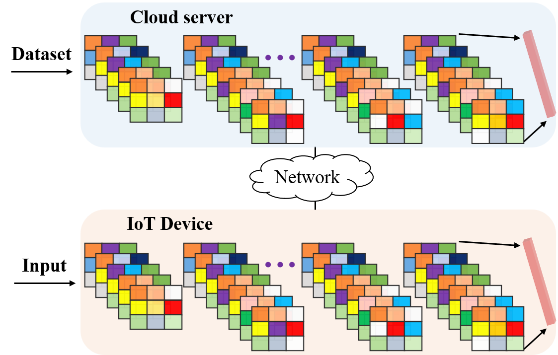
Fig. 1 shows the process of cloud-assisted CNN model training. The system architecture consists of two components: IoT devices and cloud servers. The deep CNN model is trained in the cloud server and then sent to the IoT device to provide users with services. When the subsequent CNN model is updated, the cloud server will periodically deliver the updated model to the IoT device. To combine ubiquitous IoT devices with high-performance CNN models and provide users with high-quality services this paper will study the cloud-assisted training of CNN models.
Challenges. Implementing cloud-assisted training of a CNN model system is a nontrivial task that faces the following two key challenges: The first key challenge is to reduce the model parameters sent by the cloud server to the IoT devices. The cloud server usually assists hundreds of millions of IoT devices in deploying and updating CNN models. In addition, the number of parameters of the deep CNN model is high. During model training or subsequent model updating, frequent and large numbers of model parameter exchanges will place considerable pressure on the network bandwidth. Therefore, reducing the amount of model parameter transmission is a prerequisite for the smooth progress of cloud-assisted training of CNN models in the era of the Internet of Everything.
The second key challenge arises from enhancing the robustness of the CNN model on the IoT device. Due to the universality of the distribution of IoT devices, the input data for the execution of tasks are prone to degradation of CNN model performance due to environmental influence or man made malicious attacks. For example, the image data obtained on a rainy or a snowy day or the image is slightly enlarged, or some pixels are removed. Ensuring the robustness of the CNN model is a practical problem. The robustness of a model in this paper refers its generalization performance against corrupted data. Therefore, ensuring the robustness of the CNN models deployed on IoT devices is the key to its deployment.
Our solutions. To address the first challenge, we propose MonoCNN. In MonoCNN, we only learn a single filter in each layer, referred to as the seed filter, and generate the other parameters of the layer through a seed filter and filter generation function (FGF). The parameters of FGF are randomly generated and fixed, which allows them to be reproducible with a few random seeds. Therefore, the cloud server only needs to send these seed filters and random seeds to the IoT device, and the trained MonoCNN model can be reproduced on the IoT device. Compared with sending all the model parameters, sending these seed filters and seeds can significantly reduce the number of parameters transmitted from the cloud server to the IoT device.
To address the second challenge, we propose that the parameters of the MonoCNN do not completely depend on the training data. In the MonoCNN, only the parameters of the seed filter are obtained through training, and the other parameters are obtained through FGF. This makes MonoCNN affected not only by the training data but also by the rules of the FGF. As a result, our MonoCNN naturally avoids overfitting through FGF regularization so that it has better generalization when inputting corrupted data. We also investigate five FGFs and find that the monomial function significantly outperforms the others.
In summary, our main contributions are as follows:
- •
To the best of our knowledge, this is the first work that seeks to reduce model parameter transmission when training CNN models in a cloud-assisted way. Our key idea is to issue only a small number of seed filters and seeds and improve model robustness by incorporating filter generation function rules.
- •
We perform a theoretical analysis of the MonoConv layer, showing that it can approximate the standard convolutional layer well.
- •
The experimental results show that the proposed framework reduces a large amount of model parameter transfer between the cloud server and the IoT device and improves the mean accuracy by approximately 2.2% when dealing with corrupted data.
II Related Work
Combining cloud servers, Internet of Things (IoT) devices, and deep neural network models to provide users with high-quality services has become mainstream. We group existing work into three categories (cloud-only, device-only, and cloud-device collaboration) based on where the neural network model training and inference are performed.

Cloud-only: The key desiderata of generating a high-performance neural network model are sufficient computing resources and sufficient training data. The configuration of the cloud server perfectly matches these desiderata, which introduced research on running neural network models in the cloud server [12, 13, 14, 15]. Among them, Jiang et al. [12] proposed a video analysis controller based on cloud and deep neural networks. Liu et al.. [13] proposed a deep learning-based food recognition system that runs a deep neural network model in the cloud, and the device obtains recognition services by uploading the collected data to the cloud. To reduce the quantity of data uploaded to the cloud, they also incorporate edge computing to process data on edge servers [16, 17, 18]. However, cloud execution is highly dependent on network conditions. When network conditions are unstable or disconnected, cloud-based deep neural network models become degraded or unavailable.
Device-only: With the enhancement of computing and storage capabilities of IoT devices, it is possible to train neural network models directly on IoT devices, which has also led to the birth of many excellent lightweight models, such as MobileNets [19, 20, 21], resource-aware models [22], inference efficiency [23, 24] and others [25]. For example, Howard et al. [19] used depthwise separable convolution instead of standard convolution to reduce the number of parameters in the network model. Fang et al. [22] deployed many models on end-devices and nested these models together to provide users with multiple model choices while saving storage and switching overhead. Teerapittayanon et al. [24] and Fang et al. [23] introduced an early exit and multi-branch network to improve the efficiency of inference. The above methods explore how to modify the neural network model to adapt to the IoT device or better training or inference. Hence they are complementary to our proposed approach.
Cloud-device collaboration: Research on cloud-device collaborative training and inference has received high levels of attention with a large number of excellent approaches [26, 27, 28, 29, 30, 31, 32, 33] have been proposed. For example, Zhang et al. [26] train the neural network model through cloud-edge collaboration and prune the deep neural network in the cloud to minimize the number of model transmission parameters while retaining the original model performance to the greatest extent. Stefanos et al. [27] proposed a progressive inference method for collaborative device and cloud computing and used compression [34] and quantization [35] to reduce the amount of parameter exchange between the device and the cloud. Kang et al. [30] divided the CNN into a head that runs on the device and a tail that runs on the cloud and decided the split point according to the load of the device and the cloud and network conditions. Akin, Li et al. [32] proposed a joint accuracy and latency-aware execution framework, which explores the splitting points of neural network models so that one part runs on edge devices and the other part runs in the cloud, achieving fewer parameter exchanges. The above methods have made great contributions to reducing model parameter exchange. However, some methods reduce the exchange of model parameters by finding the best splitting point. Since the optimal splitting points of different models are different, it is time-consuming and labor-intensive to search for suitable splitting points. In addition, reducing the transmission of model parameters through compression and quantization results in a loss in model performance.
In contrast, our proposed approach only requires the cloud server to send one seed filter and one seed for each layer in MonoCNN to the IoT device, which solves the overload of network transmission bandwidth caused by excessive model parameter transmission. In addition, we also address the challenge of ensuring model robustness, which is ignored by the above approaches, by using rules to regularize the generation of model parameters.
III Design of the proposed approach
III-A Overview
Fig. 2 illustrates the architecture of the proposed framework. In our framework, we first train MonoCNN in the cloud server. Instead of learning all the parameters of MonoCNN, we only learn a single filter in each layer, referred to as the seed filter. Other parameters of each layer are generated by its corresponding seed filter and filter generation function (FGF) and can be reproduced through a random seed. Therefore, the cloud server only sends a small number of seed filters and seeds to the IoT device. After obtaining seed filters and seeds, the IoT device uses them to generate multiple novel filters and combine them into the MonoCNN trained on the cloud server. We describe the proposed framework in detail as follows: ①: the cloud-assisted method in Section III-B, ②: seed filter learning in Section III-C, and ③: the filter generation function in Section III-D.
III-B Design of cloud-assisted method
Our goals are threefold i) leverage the complete resources of cloud servers, ii) limit the demand for resources on IoT devices, and iii) minimize the amount of model parameter transmission. To facilitate this goal, we propose training MonoCNN on the cloud server first and then sending the trained model to the IoT device for deployment. In general, one cloud server corresponds to millions of IoT devices. We train MonoCNN on the cloud server and then send the trained MonoCNN to IoT devices, which facilitates updating and maintaining our model on the IoT device.
III-C Design of seed filter learning
Existing high-performance CNN models have a large number of parameters. For example, VGG19 [1] has 144 million parameters. In addition, one cloud server corresponds to millions of IoT devices. Thus a large number of model parameters still need to be transmitted to IoT devices. To this end, we start with an analysis of the CNN model parameters. As [36] shows, the standard CNN model contains many redundant parameters [2]. To reduce the number of learnable parameters in the CNN model, [36] first generates several filters and then generates some novel filters through inexpensive operations. Juefei et al. [37] decomposed a standard convolutional layer into two modules, a nonlearnable layer, and a convolutional layer. Introducing the nonlearnable layer may represent a breakthrough in reducing the number of model parameters sent by the cloud server to the IoT devices. This is because the nonlearnable parameters are randomly initialized and can simply be saved and reproduced from a random seed. The nonlearnable parameters in this paper refer to the parameters in the CNN model that remain unchanged during training and inference and remain unchanged during model training on the cloud server.
The above analysis inspires us to specify that the parameters of only one filter (called the seed filter) in each layer of the CNN model should be learnable while the parameters of all other filters are nonlearnable and are generated per certain rules based on the seed filter. In this paper, we refer to this CNN as MonoCNN. Formally, in any given layer, given the seed for that layer, we can generate many new filters. The filters are generated via certain specified rules, e.g., a nonlinear transformation , where is a monomial that operates on each element of and is the exponent. The convolutional outputs are computed as follows (we consider 1-D signals for simplicity):
| (1) |
where is the channel of the input image and is the channel of the filter. During the forward pass, weights are generated from the seed filter and are then convolved with the inputs, i.e.,
| (2) | ||||
| (3) |
where we normalize the response maps to prevent the responses from vanishing or exploding and is the normalized response map.
Therefore, for a layer in MonoCNN, by specifying a seed filter along with certain rules (e.g., monomial functions), we can generate or augment as many filters as needed. For example, assume that we need filters in total for one layer, where these filters are nonlearnable and are pointwise monomial transformations of the seed filter . The input image is filtered by these filters to generate response maps, which are then passed through a nonlinear activation gate, such as a rectified linear unit (ReLU) [38], and become feature maps. Accordingly, the process of generating the feature maps can be expressed as,
| (4) |
where is a nonlinear activation, and is the monomial filter.

Compared to a standard CNN module with the same structure (with convolutions), the number of learnable parameters is significantly smaller in the MonoCNN model. Let us assume that the numbers of input and output channels are and , respectively. Therefore, the size of each 3-D filter in both the CNN and the proposed MonoCNN is , where is the kernel size of the filter, and there are such filters. The convolutions act on the filters and create the -channel output. For the standard CNN, the number of learnable parameters is . For the MonoCNN model, the number of learnable parameters is . For simplicity, let us assume that , which is usually the case for a deep CNN architecture. Then, we have the parameter saving ratio:
and when the filter kernel size is and the number of convolutional filters required for each layer satisfies , we have a parameter saving ratio of . It should be mentioned that our proposed MonoCNN does not include convolutions, and thus . Consequently, the parameter saving ratio of our proposed MonoCNN becomes equal to , i.e., the number of filters per layer in the CNN model; for a high-performance CNN model, there are typically 32, 64, 256, 512, and 1024 filters per layer. Accordingly, our MonoCNN achieves parameter savings of approximately , , or more.
On the cloud server, MonoCNN contains only a few learnable parameters while other parameters of the model are randomly generated according to predefined rules and can be saved and reproduced through random seeds. Thus, after the cloud server has trained MonoCNN, the cloud server needs to send only the seed filters and the random seeds to the IoT device to reproduce the trained MonoCNN. Compared to transmitting all model parameters, sending only seed filters and random seeds can significantly reduce communication costs.
We further explore the use of a stagewise supervised training paradigm to assist in training the MonoCNN model. Fig. 3 depicts the training pipeline. Specifically, given a MonoCNN model as a student model, we use its counterpart CNN model (a standard CNN) as a teacher model. We group the network layers into multiple stages, such that feature maps of the same size (i.e., spatial resolution) belong to the same stage while reducing the feature map size by half in each subsequent stage. Let denote the output feature maps of the teacher model in the -th stage, and let denote the output feature maps of the student (i.e., MonoCNN) model in the -th stage. We use the -norms between and as additional losses to supervise the intermediate feature learning process. In addition, we leverage knowledge distillation (KD) [39], taking the output probabilities from the teacher model as soft labels. Therefore, the final loss that we backpropagate for training the MonoCNN model is defined as follows:
where and denote the inputs and outputs, respectively, provided by the dataset; denotes the learnable parameters of the MonoCNN model (i.e., the seed filter parameters); and are the output probabilities of the teacher model and the student (i.e., MonoCNN) model, respectively; and is the cross-entropy loss. Note that we also add -norms of the learnable parameters to prevent overfitting, which are removed in the above loss formulation for brevity. See Fig. 3 for a pictorial illustration.
Fig. 4 illustrates the performance and convergence rates of the standard CNN model, the MonoCNN model without KD, and the MonoCNN model on the CIFAR-10 dataset. As shown in Fig. 4(a), when processing clean data, the MonoCNN model converges faster than the standard CNN model, but the performance is lower. However, when KD is used performance of MonoCNN model improves, and its convergence rate decreases, possibly due to the use of a standard CNN as the teacher model. As shown in Fig. 4(b), when processing corrupted data, the three methods achieve comparable convergence rates. The performance of the MonoCNN model is higher than that of the standard CNN model and slightly higher than that of the MonoCNN model without KD. The experimental results shown in Fig. 4 demonstrate the superiority of the MonoCNN model in handling corrupted data.
III-D Filter generation function design
The combination of using seed filters and generating new filters according to certain rules makes MonoCNN comparable to or exceeds the performance of the standard CNN model in handling corrupted data. The rules for generating new filters are of great merit. The standard CNN model contains a large number of nonlinear mappings, which inspired us to use nonlinear mapping functions as FGFs. Given the existing nonlinear mapping functions and the large number of derivations included in the standard CNN model, we choose the following five functions that are easy to compute:
| (5) |
| (6) |
| (7) |
| (8) |
| (9) |
Eq. 5, Eq. 6, Eq. 7, Eq. 8 and Eq. 9 are monomial function, Gaussian function, multiquadric function, inverse quadratic function and inverse multiquadric function, respectively. These functions are nonlinear and easy to compute after derivation. Since a theoretical basis to prove which nonlinear mapping function is the best for generating novel filters proved elusive we empirically evaluate them across different datasets. As shown in Fig. 5, and the monomial function is significantly better than the others in terms of performance. Therefore, we use the monomial function in our FGF in this paper and call the CNN model based on the seed filter and monomial function as MonoCNN.
III-E Discussion
III-E1 Using MonoCNN on IoT devices
After the IoT device receives the seed filters and seeds sent by the cloud server, there are two methods for using MonoCNN. The first method is to generate the MonoCNN according to the seed filters, seeds and the FGF when the IoT is idle and store it. When the MonoCNN model needs to be used, the IoT device can page it into memory to run it in the same way as the standard CNN model. The second method is to dynamically generate the MonoCNN model. That is, when the MonoCNN needs to be used, the IoT device instantly generates the MonoCNN by paging the seed filters, seeds, and the FGF into memory. The second method, which only stores seed filters and seeds on the IoT device, can save memory usage and page-in overhead. However, the price is that there is a certain overhead in generating the MonoCNN model. Practically, since the generation process of MonoCNN has only one multiplication and addition operation, its generation overhead is small. We will test the resource overhead of generating MonoCNN on the IoT device as our future work.
III-E2 Theoretical analysis
Here, we provide theoretical analysis on the MonoConv layer and demonstrate how it can well approximate the standard convolutional layer.
At layer , let be a vectorized single patch from the -channel input maps at location , where is the kernel size of the convolutional filter. Let be a vectorized single convolution filter from the convolutional filter tensor , which contains a total of generated convolutional filters at layer . We drop the layer subscription for brevity.
In a standard CNN, this patch is taken as a dot product with the filter , followed by the nonlinearity (e.g., ReLU ), resulting in a single output feature value at the corresponding location on the feature map. Similarly, each value of the output feature map is a direct result of convolving the entire input map with a convolutional filter . This microscopic process can be expressed as:
| (10) |
Without loss of generality, we assume a single-seed MonoConv case for the following analysis. For a MonoConv layer, a single-seed filter is expanded into a set of convolutional filters where , and the exponents s are predefined and are not updated during training.
The corresponding output feature map value from a MonoConv layer is a linear combination of multiple elements from the intermediate response maps. Each slice of this response map is obtained by convolving the input map with , followed by a nonlinearity. The corresponding output feature map value is thus obtained by linearly combining the response maps with parameters . This entire process can be expressed as:
| (11) |
where is now a 2D matrix of size with filters stacked as rows, with a slight abuse of notation. . Comparing and , we consider the following two cases (i) : since , there always exists a vector such that . However, when (ii) , it is obvious that the approximation does not hold when . Thus, under the assumption that is not an all-zero vector, the approximation will hold.
| Method | Params (M) | Top-1 Accuracy (%) | |
| CIFAR-10 | CIFAR-100 | ||
| CNN | 9.2 | 92.44±0.19 | 71.69±0.10 |
| LBCNN | 1.2 | 87.67±0.30 | 60.57±0.10 |
| PNN | 1.2 | 70.61±0.17 | 43.56±0.10 |
| ShiftNet | 1.1 | 30.83±0.88 | 8.84±0.46 |
| GhostNet | 4.9 | 90.05±0.25 | 65.59±0.19 |
| MonoCNN | 2.4 | 91.45±0.15 | 69.17±0.21 |
| Method | Params (M) | Top-1 Accuracy (%) | |
| CIFAR-10 | CIFAR-100 | ||
| CNN | 11.2 | 95.19±0.11 | 77.98±0.33 |
| LBCNN | 2.8 | 93.05±0.10 | 72.72±0.02 |
| PNN | 2.8 | 92.45±0.18 | 73.21±0.13 |
| ShiftNet | 2.8 | 92.76±0.14 | 73.67±0.24 |
| GhostNet | 4.3 | 93.40±0.14 | 72.77±0.58 |
| MonoCNN | 2.8 | 94.02±0.06 | 74.22±0.13 |
| Method | Params (M) | Top-1 Accuracy (%) | |
| CIFAR-10 | CIFAR-100 | ||
| CNN | 21.3 | 95.57±0.08 | 78.73±0.42 |
| LBCNN | 3.9 | 93.54±0.16 | 73.81±0.21 |
| PNN | 3.9 | 92.31±0.20 | 73.33±0.14 |
| ShiftNet | 3.9 | 92.84±0.20 | 73.87±0.25 |
| GhostNet | 7.1 | 93.58±0.24 | 73.16±0.63 |
| MonoCNN | 4.0 | 94.24±0.12 | 75.63±0.52 |
IV Evaluation
In this section, we first introduce our experimental setup including the datasets, baselines, and evaluation metrics studied in this work, followed by the implementation details. We then provide an empirical comparison in terms of network complexity and performance on multiple vision benchmarks.
IV-A Experimental Setup
Datasets. Five popular datasets are used to verify the effectiveness of the proposed method.
CIFAR-10/-100 [40] are two multiclass natural object datasets widely used for image classification. Both consist of 50,000 training and 10,000 test images from 10/100 classes, with each image of pixels.
MS COCO [41] dataset comprises more than 100K images of diverse objects with annotations, including both bounding boxes and segmentation masks, from 80 categories. We take the train2017 set for training and compare detection performance on the val2017 set.
PASCAL VOC 2012 [42] is a comparably small-scale dataset of images with 20 foreground object categories and one category for background. Following prior works [43], we augment the original training set with the extra annotations from [44], resulting in 10, 582 images (train_aug) in total for training. We use this dataset for both object detection and semantic segmentation.
Cityscapes [45] is a large-scale (images are of pixels) dataset for semantic understanding of urban street scenes. It is officially split into a training set of 2, 975 images, a validation set of 500 images, and a (privately hosted) testing set of 1, 525 images. We use 19 from the provided 30 classes for semantic segmentation.
Baselines. To verify the effectiveness of the proposed method, we consider the following baselines:
LBCNN [37]: The local binary convolutional neural network (LBCNN) uses sparse local binary filter parameters (randomly initialized and kept fixed) followed by a learned convolution to replace regular convolution layers.
PNN [46]: The perturbative neural network (PNN) injects randomly generated additive noise to the input features combined through a learned convolution to replace regular convolution layers.
ShiftNet [47]: ShiftNet applies a sparse spatial shift (e.g., one pixel left) to create diverse viewpoints of features, replacing the regular convolutions.
GhostNet [36]: GhostNet partially substitutes computationally expensive operations (e.g., regular convolutions) with cheap operations (e.g., or grouped convolutions).
To ensure a fair and comprehensive comparison, we implement all the above baseline methods within three well-studied underlining architectures, including VGG11 [1], ResNet18 [2], and ResNet34 [2].
Evaluation Metrics. We use top-1 accuracy to compare performance for image classification. We use the mean average precision (AP), computed for a recall value over 0 to 1, for object detection. For semantic segmentation, we adopt mean intersection-over-union (mIoU), which computes the IoU for each semantic class averaged over classes. It is worth noting that we only consider the number of parameters that must be learned, as these are the parameters that must be sent from the cloud server to IoT devices.
Implementation Details. We implement our method in PyTorch 1.7 with CUDA 10.1, and all experiments are performed on 2080TI GPUs. Following the suggestions from the original papers, we set the sparsity to 0.9 for LBCNN [37] and the noise level to 0.01 for PNN [46]; we use the convolution as the cheap operation for GhostNet [36] and set the ratio to 4.
IV-B Experimental Results
In this section, we first present a comparison of network complexity, followed by a performance comparison for image classification, object detection, and semantic segmentation on clean data. Finally, we compare robustness on limited training data, corrupted data, and different style data.
IV-B1 Amount of Model Parameter Transmission
Our proposed MonoCNN minimizes the number of model parameters sent by the cloud server to IoT devices. As shown in Fig. 6, we consider three widely used architectures (VGG11 and ResNet18/34) and compare the learnable parameters of MonoCNN with those of regular CNNs for image classification, object detection, and semantic segmentation. Since all filter parameters in the standard CNN model need to be learned, the cloud server needs to send all the filter parameters of the standard CNN model to the IoT device, resulting in a large amount of model parameter transmission. In contrast, in our proposed MonoCNN, only a single-seed filter needs to be learned in each layer, and the rest of the filters are generated by the filter generation function. The hyperparameters of the filter generation function (e.g., monomial exponent) are randomly initialized and remain fixed so that these nonlearnable hyperparameters can be saved and reproduced by the random number generator seed. Therefore, cloud-assisted training of MonoCNN only requires the cloud server to send a few seed filters and the random number generator seeds to recover the MonoCNN model on the IoT device.
Additionally, as shown in Fig. 6, GhostNet also has fewer model parameters than the standard CNN model because GhostNet uses cheap operations to augment filters. However, our proposed MonoCNN needs to send fewer model parameters, and in subsequent experiments, our proposed MonoCNN outperforms GhostNet in almost all tasks. It is worth mentioning that other types of parameter reduction techniques (e.g., pruning, quantization [34], and neural architecture search [48, 49]) can be applied on top of our method for further compression of model parameters.
IV-B2 Results on Standard Benchmarks
In this section, we evaluate the effectiveness of our MonoCNN on standard benchmark datasets for image classification, object detection, and semantic segmentation tasks.
Image Classification. For training on the CIFAR-10/-100 datasets, we use the SGD optimizer with an initial learning rate of 0.025, which is annealed to zero following the cosine schedule. We use standard data augmentations: we pad images with four pixels on each side and randomly crop a region, from which random horizontal flipping is also applied. Given the stochastic nature of the CIFAR datasets (as the results are subject to high variance even with exactly the same setup), we repeat the training five times with different initial random seeds and report the mean performance along with the standard deviation.
Table I depicts the results. In general, we observe that our MonoCNN consistently outperforms other peer methods on both CIFAR-10 and CIFAR-100 while requiring a similar or fewer number of parameters to be learned. Additionally, our MonoCNN provides substantial savings in the parameters while achieving similar accuracy performance when compared to regular CNNs. In particular, the proposed MonoCNN is 3.58% more accurate on CIFAR-100 and 2 more compact than GhostNet [36] when paired with the VGG11 architecture.
Objection Detection. To evaluate the effectiveness of our model for object detection, we implement all compared methods using ResNet18 as the underlining backbone architecture and FPN [50] as the detection head. For training on both MS COCO and PASCAL VOC 2012, we use the SGD optimizer with an initial learning rate of 0.02 and a batch size of eight over four GPU cards. Following the common practice, we adopt the 1 (i.e., 12 or 36 epochs) schedule to train our detection models and decay the learning rate at the 8th and 11th epochs by a factor of 10. We resize the training images to the shorter side of 800 pixels with the longer side to be within 1333 pixels for MS COCO. We resize the training images to for PASCAL VOC 2012.
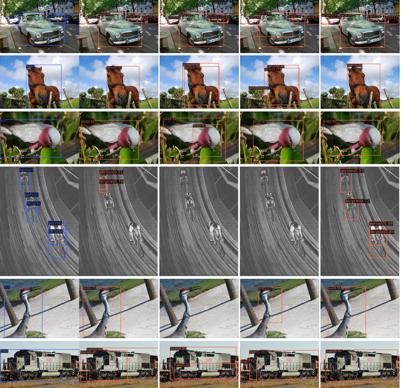
Table II and Table III depict the results. Similar to the previous case of image classification, the proposed MonoCNN consistently outperforms other peer methods for object detection. In particular, MonoCNN achieves 6.2 and 8.0 higher AP points than LBCNN [37] while using a similar number of parameters. In addition, we also provide a qualitative visualization between MonoCNN and the compared methods in Fig. 7. Evidently, MonoCNN (right-most column in Fig. 7) is not only more accurate in detecting smaller objects (see the first and fourth row in Fig. 7) but also more precise in avoiding duplicate detection boxes (see second and third row in Fig. 7) than peer methods (Columns 2-4 in Fig. 7).
| Method | AP | AP50 | AP75 | APs | APm | APl |
| CNN | 33.1 | 52.6 | 35.5 | 18.9 | 35.4 | 43.1 |
| LBCNN | 25.6 | 43.3 | 26.3 | 13.4 | 27.2 | 34.2 |
| GhostNet | 30.4 | 49.3 | 32.1 | 16.8 | 32.5 | 40.8 |
| MonoCNN | 31.8 | 51.3 | 34.1 | 17.3 | 33.9 | 41.9 |
| Method | AP | AP50 | AP75 | APs | APm | APl |
| CNN | 47.4 | 79.8 | 50.6 | 19.1 | 33.9 | 52.1 |
| LBCNN | 37.7 | 69.5 | 36.1 | 18.0 | 25.1 | 41.8 |
| GhostNet | 44.3 | 76.7 | 45.9 | 17.2 | 31.1 | 48.8 |
| MonoCNN | 45.7 | 78.1 | 47.7 | 16.5 | 30.8 | 50.8 |
Semantic Segmentation. We follow the same setup as in the previous case of object detection. We also implement all compared methods using ResNet18 as the underlining backbone architecture and FPN as the segmentation head. For training on Cityscapes and PASCAL VOC 2012, we use the SGD optimizer with a momentum of 0.9 and weight decay of 5e-4. The batch size is set to 24 over two 2080TI GPUs. Following the common practice, we adopt the “poly” learning rate policy (i.e., ) from 0.01 to zero in 60K iterations. Data augmentation includes color jittering, random horizontal flipping, random cropping and random resizing. In addition, we scale training images with a factor randomly sampled from [0.125, 1.5] and crop them to for Cityscapes.
Table IV and Table V break down the classwise segmentation mIoU for PASCAL VOC 2012 and Cityscapes, respectively. Evidently, we observe that our MonoCNN significantly outperforms peer competitors on both datasets. In particular, MonoCNN achieves better mIoU with 3 fewer parameters than the regular CNN model on PASCAL VOC 2012; MonoCNN achieves 3.6 and 5.2 points higher mIoU than LBCNN [37] on the two datasets, respectively. A qualitative comparison is also provided in Fig. 8. Visually, we observe that MonoCNN leads to a more fain-grained segmentation on small objects (see boxed regions in 8(a)).


| Method | aero | bike | bird | boat | bottle | bus | car | cat | chair | cow | table | dog | horse | mbike | person | plant | sheep | sofa | train | tv | mIoU |
| CNN | 79.6 | 37.4 | 71.4 | 51.3 | 54.2 | 81.5 | 76.5 | 77.6 | 28.1 | 59.9 | 38.3 | 67.8 | 66.6 | 71.7 | 78.4 | 39.2 | 66.4 | 34.4 | 69.7 | 60.4 | 65.2 |
| LBCNN | 71.8 | 35.0 | 58.8 | 47.0 | 47.1 | 76.4 | 73.0 | 72.4 | 21.4 | 46.9 | 37.8 | 59.5 | 51.4 | 63.8 | 71.4 | 31.5 | 64.0 | 30.5 | 65.4 | 52.3 | 61.9 |
| GhostNet | 77.4 | 36.2 | 69.3 | 48.8 | 56.4 | 78.4 | 74.7 | 75.8 | 27.1 | 59.1 | 40.8 | 66.0 | 62.6 | 68.5 | 76.0 | 36.3 | 66.5 | 31.3 | 68.4 | 58.8 | 63.5 |
| MonoCNN | 83.9 | 37.8 | 78.2 | 53.3 | 58.8 | 89.5 | 77.9 | 82.8 | 31.2 | 58.9 | 38.3 | 71.6 | 71.8 | 75.0 | 77.6 | 48.2 | 73.9 | 35.2 | 77.4 | 63.7 | 65.5 |
| Method | road | sidewalk | building | wall | fence | pole | light | sign | vegetation | terrain | sky | person | rider | truck | bus | caravan | trailer | train | motorcycle | mIoU |
| CNN | 97.3 | 78.8 | 89.9 | 50.1 | 47.4 | 47.4 | 55.5 | 66.8 | 89.9 | 58.6 | 93.0 | 72.7 | 50.3 | 92.4 | 63.3 | 74.0 | 53.4 | 51.0 | 67.9 | 68.4 |
| LBCNN | 96.9 | 76.4 | 88.2 | 47.8 | 42.3 | 40.6 | 44.2 | 59.9 | 88.6 | 56.3 | 92.1 | 66.8 | 42.2 | 90.6 | 56.2 | 65.2 | 36.1 | 41.6 | 63.6 | 62.9 |
| GhostNet | 97.3 | 79.4 | 89.2 | 47.9 | 46.5 | 45.7 | 51.7 | 64.7 | 89.6 | 59.9 | 92.6 | 70.7 | 46.6 | 91.5 | 60.0 | 75.8 | 65.7 | 41.4 | 66.2 | 67.5 |
| MonoCNN | 97.4 | 79.8 | 89.7 | 49.0 | 48.7 | 46.0 | 55.0 | 65.7 | 90.0 | 61.0 | 93.0 | 71.3 | 49.1 | 92.1 | 66.4 | 73.0 | 58.9 | 39.4 | 66.5 | 68.1 |
Discussion. As shown by experimental results on image classification, object detection, and semantic segmentation tasks, the proposed MonoCNN consistently outperforms a wide range of existing alternatives with similar or fewer parameters. In addition, the proposed MonoCNN can significantly decrease the number of parameters compared to standard CNN models, but with slight performance degradation. The main reason is that it is difficult for MonoCNN with a small number of learnable parameters to process the test images that are highly correlated with the training images through the training images. However, in real scenarios, in the data collected by IoT devices, the correlation between training images and test images is much smaller than that of the training image set and test image set divided by the standard dataset. For MonoCNN, its parameters are also affected by the filter generation function and are not completely dependent on the training data, thus MonoCNN is expected to achieve high performance in processing this type of image.
IV-B3 Results on Robustness
In this section, we use CIFAR-10 classification to evaluate the performance of the proposed MonoCNN for robustness on limited data and on data with commonly observable corruptions.
Limited training data. Insufficient training data are a conventional difficulty for deep neural network models but often arise in practical applications. Considering the lower model complexity (i.e., fewer learnable parameters), we hypothesize that MonoCNN may be less prone to overfitting to the limited training data. To verify this hypothesis, we perform an empirical experiment on (randomly selected) subsets of the CIFAR-10 training set while keeping the testing set intact. Fig. 9 depicts the results. Compared to fully learned convolutions (standard CNNs), MonoCNN exhibits noticeably better generalization performance under limited training data.
| Group | Corruption Types | |
| Noise |
| |
| Blur |
| |
| Weather |
| |
| Digital | Contrast, Elastic, JPEG compression, Pixelate, Saturate |


Corrupted data. The vulnerability to a small perturbation in inputs adversely affects the deployment of deep learning vision systems in many IoT applications that are sensitive to safety and user privacy. To quantitatively measure the robustness of the proposed MonoCNN, we consider the CIFAR-10-C dataset proposed by Hendrycks and Dietterich [51], who applied common observable corruption to the original (i.e., clean) test images of CIFAR-10. There are 19 different types of corruption from four main categories. See Table VI for details and Fig. 10 for visualization.
Based on the empirical findings summarized in Table VII, we observe that our MonoCNN performs significantly better than other peer models under a similar number of parameters. In addition, MonoCNN also performs noticeably better than the regular CNN model.
| Method | Noise | Blur | Weather | Digital | mean |
| CNN | 57.05±7.55 | 74.90±10.5 | 86.27±5.41 | 82.32±6.34 | 75.13±12.9 |
| LBCNN | 54.88±6.87 | 67.61±12.0 | 81.79±7.49 | 78.41±7.62 | 70.67±12.1 |
| PNN | 50.13±6.67 | 63.27±9.12 | 79.30±7.56 | 76.09±7.57 | 67.20±11.5 |
| GhostNet | 58.48±5.93 | 67.53±9.95 | 81.57±7.35 | 78.10±7.61 | 71.42±9.08 |
| MonoCNN | 64.41±5.42 | 77.41±9.41 | 85.31±5.01 | 82.22±6.22 | 77.34±7.98 |
Data under different styles. In addition to data under degraded quality, another important angle for measuring robustness is the generalization performance on data under different styles, i.e., data with the same context but represented differently. We consider the Icons-50 dataset [51], which consists of 10K images from 50 classes of icons (e.g., airplane, symbols, activities, etc.) collected by various technology companies (e.g., Apple, Facebook, Google, etc.). We hold off data from one company while training on data from other companies to quantify robustness under different styles. See Fig. 11 for a visualization.

As shown in Table VIII, the mean accuracy of our proposed MonoCNN outperforms the mean accuracy of other models. For example, our proposed MonoCNN achieves a mean accuracy improvement of 1.15% compared to the regular CNN. The main reason is that the parameters of MonoCNN are affected by both the filter generation function and the training data, which makes MonoCNN promising for achieving better performance than regular CNNs when dealing with test data whose style is inconsistent with the training data.
| Method | Apple | Samsung | Mean | ||
| CNN | 91.74±0.65 | 86.56±0.25 | 82.63±0.88 | 81.30±1.11 | 85.56±4.69 |
| LBCNN | 92.73±0.67 | 87.63±1.33 | 83.42±0.40 | 79.09±0.62 | 85.72±5.83 |
| PNN | 92.49±0.48 | 82.43±1.37 | 82.24±1.11 | 82.19±1.67 | 84.84±5.10 |
| GhostNet | 92.95±0.80 | 85.26±2.20 | 80.85±0.58 | 76.64±0.71 | 83.93±6.97 |
| MonoCNN | 93.52±0.59 | 86.48±0.66 | 82.42±1.61 | 84.40±0.87 | 86.71±4.84 |
In Table VII and Table VIII, we observe that when there exists sufficient training data and the test data are within the same underlining distribution as the training data, all efficiency-oriented methods (i.e., LBCNN, PNN, GhostNet, and MonoCNN) exhibit a lower performance due to lower model capacity from limited parameters. However, the proposed FGF mechanism provides an inductive bias to the training of MonoCNN, which prevents overfitting to the training data, in turn, leading to a better generalization performance under limited training data and on out-of-distribution test data (i.e., corrupted data or data under different styles).
IV-C Monomial Function Hyperparameter Study
As demonstrated in the previous sections, we empirically observe that the monomial transformation is better suited for the filter generation function. In this section, we perform parameter sensitivity analysis on the hyperparameters of the monomial transformation.
Effect of polynomial terms. Instead of a monomial, one may relax the constraint on the number of terms to include the more general case of polynomial transformation. Accordingly, we allow the number of terms to grow from one (i.e., monomial) to many terms and evaluate the performance of corresponding models on CIFAR-10 classification. We repeat each setup five times and present the results in Fig. 12. We observe that monomial transformation (i.e., number of terms equal to one) is better suited for filter generation function as opposed to polynomial transformation with many terms.
Effect of monomial exponent. Recall that we adopt the pointwise polynomial transformation as the filter generation function based on our empirical experiments. The monomial filter generation function randomly samples a (continuous-valued) exponent from , where and are the lower and upper bounds on . To understand the effect of , we set the number of channels to 64 and the number of layers to 20 for our MonoCNN and vary the lower and upper bounds of . Fig. 13 depicts the results. In general, having a diverse set of exponents (i.e.,, a larger range of bounds) leads to better performance of MonoCNN. Empirically, we identify that setting the lower bound to 1 and the upper bound to 7 yields the best performance.
V Conclusions and Future work
In this paper, we make the following two contributions. First, we propose cloud-assisted training of a CNN model framework for IoT devices by considering model parameter transmission and model robustness. Second, we propose a novel CNN architecture (i.e., MonoCNN) that reduces the number of model parameters sent by the cloud server to IoT devices by specifying only one filter that needs to be learned in each layer of MonoCNN and improves the robustness of the model by regularizing the model parameters using the filter generation function. Experimental results show that the proposed approach achieves better performance in dealing with corrupted data and minimizes model parameter transmission.
In addition, Gill et al. [52] comprehensively combed the emerging trends and future directions of AI for next-generation computing, which motivates our future work to start from the following points:
- •
We will deploy MonoCNN on the IoT device (such as the Raspberry Pi 4B) and test the resources and time it takes to generate MonoCNN based on learnable parameters, seeds, and filter generation function.
- •
Since the available resources of the IoT device are dynamically changing, we need to deploy multiple MonoCNN variants with different capacities. However, this faces two challenges: (i) how to divide multiple MonoCNN variants with different capacities and how to train these MonoCNN variants; (ii) how to reduce the storage resources occupied by deploying multiple MonoCNN variants.
- •
IoT devices usually run multiple applications simultaneously. However, resources are limited. When the IoT device cannot provide sufficient resources for each application at the same time, how to reasonably allocate resources for each application poses a challenge.
- •
Training the high-performance MonoCNN requires a large quantity of labeled data; however, unlabeled data are common in real scenarios, and how to train MonoCNN with the help of unlabeled data is a practical challenge.
- •
To avoid leakage of user-sensitive private data, training MonoCNN on the IoT device is a research direction; however, how to speed up the training of MonoCNN is a challenge.
VI Acknowledgements
This work was supported by the Fundamental Research Funds for the Central Universities (2021RC272), the National Natural Science Foundation of China (62106097), the China Postdoctoral Science Foundation (2021M691424, 2021M700364), the Research Grants Council of Hong Kong through the Theme-based Research Scheme (T-41-603/20R), and the Research Grants Council of Hong Kong through the General Research Fund (PolyU 15217919).
References
- [1] K. Simonyan and A. Zisserman, “Very deep convolutional networks for large-scale image recognition,” in Proceedings of 3rd International Conference on Learning Representations, 2015, pp. 1–14.
- [2] K. He, X. Zhang, S. Ren, and J. Sun, “Deep residual learning for image recognition,” in Proceedings of the IEEE/CVF Conference on Computer Vision and Pattern Recognition, 2016, pp. 770–778.
- [3] A. Bohlender, A. Spriet, W. Tirry, and N. Madhu, “Exploiting temporal context in cnn based multisource doa estimation,” IEEE/ACM Transactions on Audio, Speech and Language Processing, vol. 29, pp. 1594–1608, 2021.
- [4] N. Kalchbrenner, E. Grefenstette, and P. Blunsom, “A convolutional neural network for modelling sentences,” in Proceedings of 52nd Annual Meeting of the Association for Computational Linguistics, 2014, pp. 655–665.
- [5] S. Minaee, N. Kalchbrenner, E. Cambria, J. Nikzad, M. Chenaghlu, and J. Gao, “Deep learning-based text classification: A comprehensive review,” ACM Computing Surveys, vol. 54, no. 3, pp. 1–40, 2021.
- [6] H. xuan Hu, Z. Jiang, Y. Zhao, Y. Zhang, H. Wang, and W. Wang, “Network representation learning-enhanced multisource information fusion model for poi recommendation in smart city,” IEEE Internet of Things Journal, vol. 8, no. 12, pp. 9539–9548, 2021.
- [7] H. Wu, Z. Zhang, C. Guan, K. Wolter, and M. Xu, “Collaborate edge and cloud computing with distributed deep learning for smart city internet of things,” IEEE Internet of Things Journal, vol. 7, no. 9, pp. 8099–8110, 2020.
- [8] Z. Lu, S. Rallapalli, K. Chan, S. Pu, and T. L. Porta, “Augur:modeling the resource requirements of convnets on mobile devices,” IEEE Transactions on Mobile Computing, vol. 20, no. 2, pp. 352–365, 2021.
- [9] A. E. Eshratifar, M. S. Abrishami, and M. Pedram, “JointDNN: An efficient training and inference engine for intelligent mobile cloud computing services,” IEEE Transactions on Mobile Computing, vol. 20, no. 2, pp. 565–576, 2021.
- [10] X. Liang, Y. Zhang, G. Wang, and S. Xu, “A deep learning model for transportation mode detection based on smartphone sensing data,” IEEE Transactions on Intelligent Transportation Systems, vol. 21, no. 12, pp. 5223–5235, 2020.
- [11] T. Qian, C. Shao, X. Wang, and M. Shahidehpour, “Deep reinforcement learning for ev charging navigation by coordinating smart grid and intelligent transportation system,” IEEE Transactions on Smart Grid, vol. 11, no. 2, pp. 1714–1723, 2020.
- [12] J. Jiang, G. Ananthanarayanan, P. Bodik, S. Sen, and I. Stoica, “Chameleon: Scalable adaptation of video analytics,” in Proceedings of the 2018 Conference of the ACM Special Interest Group on Data Communication, 2018, pp. 253–266.
- [13] C. Liu, Y. Cao, Y. Luo, G. Chen, V. Vokkarane, M. Yunsheng, S. Chen, and P. Hou, “A new deep learning-based food recognition system for dietary assessment on an edge computing service infrastructure,” IEEE Transactions on Services Computing, vol. 11, no. 2, pp. 249–261, 2018.
- [14] E. Georganas, S. Avancha, K. Banerjee, D. D. Kalamkar, G. Henry, H. Pabst, and A. Heinecke, “Anatomy of high-performance deep learning convolutions on simd architectures,” in Proceedings of the International Conference for High Performance Computing, Networking, Storage, and Analysis, 2018, pp. 1–12.
- [15] K. M. Hazelwood, S. Bird, D. M. Brooks, S. Chintala, U. Diril, D. Dzhulgakov, M. Fawzy, B. Jia, Y. Jia, A. Kalro, J. Law, K. Lee, J. Lu, P. Noordhuis, M. Smelyanskiy, L. Xiong, and X. Wang, “Applied machine learning at facebook: A datacenter infrastructure perspective,” in Proceedings of the IEEE International Symposium on High Performance Computer Architecture, 2018, pp. 620–629.
- [16] N. Abbas, Y. Zhang, A. Taherkordi, and T. Skeie, “Mobile edge computing: A survey,” IEEE Internet of Things Journal, vol. 5, no. 1, pp. 450–465, 2018.
- [17] P. Mach and Z. Becvar, “Mobile edge computing: A survey on architecture and computation offloading,” IEEE Communications Surveys and Tutorials, vol. 19, no. 3, pp. 1628–1656, 2017.
- [18] T. Liu, Y. Zhang, Y. Zhu, W. Tong, and Y. Yang, “Online computation offloading and resource scheduling in mobile-edge computing,” IEEE Internet of Things Journal, vol. 8, no. 8, pp. 6649–6664, 2021.
- [19] A. G. Howard, M. Zhu, B. Chen, D. Kalenichenko, W. Wang, T. Weyand, M. Andreetto, and H. Adam, “Mobilenets: Efficient convolutional neural networks for mobile vision applications,” in CoRR abs/1704.04861, 2017, pp. 2464–2469.
- [20] M. Sandler, A. G. Howard, M. Zhu, A. Zhmoginov, and L.-C. Chen, “Mobilenetv2: Inverted residuals and linear bottlenecks,” in Proceedings of the IEEE/CVF Conference on Computer Vision and Pattern Recognition, 2018, pp. 4510–4520.
- [21] A. Howard, R. Pang, H. Adam, Q. V. Le, M. Sandler, B. Chen, W. Wang, L.-C. Chen, M. Tan, G. Chu, V. Vasudevan, and Y. Zhu, “Searching for mobilenetv3,” in Proceedings of IEEE/CVF International Conference on Computer Vision, 2019, pp. 1314–1324.
- [22] B. Fang, X. Zeng, and M. Zhang, “Nestdnn: Resource-aware multi-tenant on-device deep learning for continuous mobile vision,” in Proceedings of 16th Annual International Conference on Mobile Computing and Networking, 2018, pp. 115–127.
- [23] B. Fang, X. Zeng, F. Zhang, H. Xu, and M. Zhang, “Flexdnn: Input-adaptive on-device deep learning for efficient mobile vision,” in Proceedings of 5th IEEE/ACM Symposium on Edge Computing, 2020, pp. 84–95.
- [24] S. Teerapittayanon, B. McDanel, and H. T. Kung, “Branchynet: Fast inference via early exiting from deep neural networks,” in Proceedings of the IEEE/CVF Conference on Computer Vision and Pattern Recognition, 2016, pp. 2464–2469.
- [25] A. Mathur, N. D. Lane, S. Bhattacharya, A. Boran, C. Forlivesi, and F. Kawsar, “Deepeye: Resource efficient local execution of multiple deep vision models using wearable commodity hardware,” in Proceedings of the 15th Annual International Conference on Mobile Systems, Applications, and Services, 2017, pp. 68–81.
- [26] X. Zhang, M. Qiao, L. Liu, Y. Xu, and W. Shi, “Collaborative cloud-edge computation for personalized driving behavior modeling,” in Proceedings of 4th ACM/IEEE Symposium on Edge Computing, 2019, pp. 209–221.
- [27] S. Laskaridis, S. I. Venieris, M. Almeida, I. Leontiadis, and N. D. Lane, “Spinn: Synergistic progressive inference of neural networks over device and cloud,” in Proceedings of 16th Annual International Conference on Mobile Computing and Networking, 2020, pp. 1–15.
- [28] S. Teerapittayanon, B. McDanel, and H. T. Kung, “Distributed deep neural networks over the cloud, the edge and end devices,” in Proceedings of 37th IEEE International Conference on Distributed Computing Systems, 2017, pp. 328–339.
- [29] J. Ren, Y. Guo, D. Zhang, Q. Liu, and Y. Zhang, “Distributed and efficient object detection in edge computing: Challenges and solutions,” IEEE Network, vol. 32, no. 6, pp. 137–143, 2018.
- [30] Y. Kang, J. Hauswald, C. Gao, A. Rovinski, T. Mudge, J. Mars, and L. Tang, “Neurosurgeon: Collaborative intelligence between the cloud and mobile edge,” in Proceedings of Twenty-Second International Conference on Architectural Support for Programming Languages and Operating Systems, 2017, pp. 615–629.
- [31] C. Hu, W. Bao, D. Wang, and F. Liu, “Dynamic adaptive dnn surgery for inference acceleration on the edge,” in Proceedings of IEEE Conference on Computer Communications, 2019, pp. 1423–1431.
- [32] H. Li, C. Hu, J. Jiang, Z. Wang, Y. Wen, and W. Zhu, “Jalad: Joint accuracy-and latency-aware deep structure decoupling for edge-cloud execution,” in Proceedings of IEEE 24th International Conference on Parallel and Distributed Systems, 2018, pp. 671–678.
- [33] S. Han, H. Shen, M. Philipose, S. Agarwal, A. Wolman, and A. Krishnamurthy, “Mcdnn: An approximation-based execution framework for deep stream processing under resource constraints,” in Proceedings of the 14th Annual International Conference on Mobile Systems, 2016, pp. 123–136.
- [34] S. Han, H. Mao, and W. J. Dally, “Deep compression: Compressing deep neural networks with pruning, trained quantization and huffman coding,” in Proceedings of 4th International Conference on Learning Representations, 2016, pp. 1–14.
- [35] I. Hubara, M. Courbariaux, D. Soudry, R. EI-Yaniv, and Y. Bengio, “Quantized neural networks: Training neural networks with low precision weights and activations,” Journal of Machine Learning Research, vol. 18, pp. 1–30, 2017.
- [36] K. Han, Y. Wang, Q. Tian, J. Guo, C. Xu, and C. Xu, “Ghostnet: More features from cheap operations,” in Proceedings of the IEEE/CVF Conference on Computer Vision and Pattern Recognition, 2020, pp. 1577–1586.
- [37] F. Juefei-Xu, V. Naresh Boddeti, and M. Savvides, “Local binary convolutional neural networks,” in Proceedings of the IEEE/CVF Conference on Computer Vision and Pattern Recognition, 2017, pp. 4284–4293.
- [38] V. Nair and G. E. Hinton, “Rectified linear units improve restricted boltzmann machines,” in Proceedings of the 27th International Conference on Machine Learning, 2010, pp. 807–814.
- [39] G. E. Hinton, O. Vinyals, and J. Dean, “Distilling the knowledge in a neural network,” in CoRR abs/1503.02531, 2015, pp. 1–9.
- [40] A. Krizhevsky, G. Hinton et al., “Learning multiple layers of features from tiny images,” Citeseer, Tech. Rep., 2009.
- [41] T.-Y. Lin, M. Maire, S. Belongie, J. Hays, P. Perona, D. Ramanan, P. Dollár, and C. L. Zitnick, “Microsoft coco: Common objects in context,” in Proceedings of the European Conference on Computer Vision, 2014, pp. 740–755.
- [42] M. Everingham, S. A. Eslami, L. Van Gool, C. K. Williams, J. Winn, and A. Zisserman, “The pascal visual object classes challenge: A retrospective,” International journal of computer vision, vol. 111, no. 1, pp. 98–136, 2015.
- [43] C. Liu, L.-C. Chen, F. Schroff, H. Adam, W. Hua, A. L. Yuille, and L. Fei-Fei, “Auto-deeplab: Hierarchical neural architecture search for semantic image segmentation,” in Proceedings of the IEEE/CVF Conference on Computer Vision and Pattern Recognition, 2019, pp. 82–92.
- [44] B. Hariharan, P. Arbeláez, L. Bourdev, S. Maji, and J. Malik, “Semantic contours from inverse detectors,” in Proceedings of the IEEE International Conference on Computer Vision, 2011, pp. 991–998.
- [45] M. Cordts, M. Omran, S. Ramos, T. Rehfeld, M. Enzweiler, R. Benenson, U. Franke, S. Roth, and B. Schiele, “The cityscapes dataset for semantic urban scene understanding,” in Proceedings of the IEEE/CVF Conference on Computer Vision and Pattern Recognition, 2016, pp. 3213–3223.
- [46] F. Juefei-Xu, V. N. Boddeti, and M. Savvides, “Perturbative neural networks,” in Proceedings of the IEEE/CVF Conference on Computer Vision and Pattern Recognition, 2018, pp. 3310–3318.
- [47] W. Chen, D. Xie, Y. Zhang, and S. Pu, “All you need is a few shifts: Designing efficient convolutional neural networks for image classification,” in Proceedings of the IEEE/CVF Conference on Computer Vision and Pattern Recognition, 2019, pp. 7241–7250.
- [48] Z. Lu, G. Sreekumar, E. Goodman, W. Banzhaf, K. Deb, and V. N. Boddeti, “Neural architecture transfer,” IEEE Transactions on Pattern Analysis and Machine Intelligence, vol. 43, no. 9, pp. 2971–2989, 2021.
- [49] Z. Lu, I. Whalen, Y. Dhebar, K. Deb, E. D. Goodman, W. Banzhaf, and V. N. Boddeti, “Multiobjective evolutionary design of deep convolutional neural networks for image classification,” IEEE Transactions on Evolutionary Computation, vol. 25, no. 2, pp. 277–291, 2021.
- [50] T.-Y. Lin, P. Dollár, R. Girshick, K. He, B. Hariharan, and S. Belongie, “Feature pyramid networks for object detection,” in Proceedings of the IEEE/CVF Conference on Computer Vision and Pattern Recognition, 2017, pp. 936–944.
- [51] D. Hendrycks and T. Dietterich, “Benchmarking neural network robustness to common corruptions and perturbations,” in Proceedings of the International Conference on Learning Representations, 2019, pp. 1–16.
- [52] S. S. Gill, M. Xu, C. Ottaviani, P. Patros, R. Bahsoon, A. Shaghaghi, M. Golec, V. Stankovski, H. Wu, A. Abraham, M. Singh, H. Mehta, S. K. Ghosh, T. Baker, A. K. Parlikad, H. Lutfiyya, S. S. Kanhere, R. Sakellariou, S. Dustdar, O. Rana, I. Brandic, and S. Uhlig, “Ai for next generation computing: Emerging trends and future directions,” Internet of Things, vol. 19, no. 2, pp. 1–34, 2022.