Institute of Quantum Computing and Computer Theory, School of Computer and Engineering, Sun Yat-sen University, Chinalilvzh@mail.sysu.edu.cn[orcid][funding] Institute of Quantum Computing and Computer Theory, School of Computer and Engineering, Sun Yat-sen University, Chinaluojq25@mail2.sysu.edu.cn[orcid][funding] Institute of Quantum Computing and Computer Theory, School of Computer and Engineering, Sun Yat-sen University, Chinaxuyzh23@mail2.sysu.edu.cn[orcid][funding]
Playing Mastermind on quantum computers The authors are ordered alphabetically.
Abstract
From the 1970s up to now, the classic two-player game, Mastermind, has attracted plenty of attention, not only from the public as a popular game, but also from the academic community as a scientific issue. Mastermind with positions and colors is formally described as follows. The codemaker privately chooses a secret , and the codebreaker want to determine in as few queries like as possible to the codemaker. is called a black-peg query if , and a black-white-peg query if , where indicates the number of positions where and coincide and indicates the number of right colors but being in the wrong position. The complexity of a strategy is measured by the number of queries used.
In this work we study playing Mastermind on quantum computers in both non-adaptive and adaptive settings, obtaining efficient quantum algorithms which are all exact (i.e., return the correct result with certainty) and show huge quantum speedups. The contributions are as follows. (i) Based on the discovery of new structure information, we construct two non-adaptive quantum algorithms which determine the secret with certainty and consume and at most black-peg queries, respectively. (ii) If adaptive strategies are admitted, a more efficient exact quantum algorithm is obtained, which consumes only black-peg queries. Furthermore, we prove that any quantum algorithm requires at least black-peg queries. (iii) When black-white-peg queries are allowed, we propose an adaptive exact quantum algorithm with queries, where is the set of colors occupied by . This algorithm breaks through the lower bound when . (iv) Technically, we develop a three-step framework for designing quantum algorithms for the general string learning problem, which not only allows huge quantum speedups on playing Mastermind, but also may shed light on exploring quantum speedups for other string learning problems.
Our results show that quantum computers have a substantial speedup over classical computers on playing Mastermind. In the non-adaptive setting, when , the classical complexity is and when the current best classical algorithm has complexity . In the adaptive setting, the classical complexity is . Therefore, significant gap between quantum and classical computing on playing Mastermind is clearly visible.
ccs
Theory of computation Quantum query complexityccs
Applied computing Computer gamesccs
Theory of computation Algorithmic game theorykeywords
Mastermind, query complexity, quantum algorithms1 Introduction
One of the core issues in the field of quantum computing is to discover more problems that admit quantum speedups, and to further design explicit quantum algorithms for these problems. Mastermind seems a good candidate for such problems, since the research on Mastermind in classical computing has continued since the 1970s and is intricate, which indicates that the structure of the problem is elusive from the perspective of classical computing, whereas in this paper we will obtain more efficient quantum algorithms with huge quantum speedups.
Mastermind is a classic board game invented in 1970 by the Israeli telecommunication expert Mordechai Meirowitz and can go back to the early work of Erdős and Rényi [19] in 1963. As mentioned in [40], before the commercial board game version of Mastermind was released in 1971, variations of this game have been played earlier under other names, such as the pen-and-paper based games of Bulls and Cows, and Jotto. The game has been played on TV as a game show in multiple countries under the name of Lingo. Recently, a similar web-based game has gained much attention under the name of Wordle.

In the commercial version of Mastermind, as shown in Figure 1, there are four pegs (positions), each of which could be selected from a set of six colors. The codemaker secretly chooses a color combination of four pegs. The goal of the codebreaker is to identify the secret in as few guesses as possible. In each round, he guesses a color combination of length to tell the codemaker, and he receives two numbers (i.e., formally defined later) about how similar the guess is to the secret. In 1977, Knuth [35] proved that queries are sufficient for a deterministic algorithm to identify the secret. In 1983, Chvátal [12] first studied the generalized version of Mastermind, i.e. positions and colors, which will be the topic of this paper. In the following, we first recall the formal definition.
1.1 Mastermind
Let throughout this paper. The Mastermind game with positions and colors is formally described as follows. At the start of the game, the codemaker chooses a secret string . In each round, the codebreaker guesses a string and the codemaker replies with or . The codebreaker “wins” the game if he gets the secret string , with the goal being to win the game by using as few queries to or as possible. When we mention “complexity” in this paper, it always means the number of queries used by the codebreaker. We call the game Black-peg Mastermind when only the black-peg query is allowed, and Black-white-peg Mastermind otherwise. It’s obvious that any algorithm for Black-peg Mastermind works for Black-white-peg Mastermind, but the reverse is not true.
- (a)
Black-peg query: A black-peg query means an invocation to the function associated with that returns for any indicating the number of positions where and coincide.
- (b)
Black-white-peg query: Similarly, a black-white-peg query means an invocation to the function that returns for any , with indicating the number of right colors but being in the wrong position, where denotes the set of all permutations of the set .
Mastermind has sparked a flurry of research, with scholars studying different variations. The components of variations are as follows [12, 5]:
- •
The color number and the position number . For example, the original version considered by Knuth [35] is with and . When , the problem reduces to identifying a binary string, and the problem considered by Erdős and Rényi [19] is essentially equivalent to this problem. The degree to which people understand the complexity of Mastermind depends on the relationship between and . Thus, the following cases were usually separately considered in classical computing: , with , and . In quantum computing, the distinction among these different cases seems unnecessary.
- •
The types of query information. The game is called Black-peg Mastermind when only the black-peg query is allowed, and Black-white-peg Mastermind otherwise. From the definitions, it can be seen that the black-white-peg query offers more information than the black-peg query, which has also been strictly verified in classical computing, since Black-white-peg Mastermind has a lower complexity than the corresponding black-peg version as shown in [17, 40, 39]. The similar phenomenon also exists in the quantum situation as will be shown in this paper.
- •
The query strategy. Depending on the strategy of how an algorithm makes a query, algorithms can be divided into two kinds: adaptive and non-adaptive. In the adaptive strategy, the queries can be made sequentially one by one, and the next query can depend on the previous queries and the answers. In the non-adaptive strategy, all the query strings must be supplied in parallel at once, and then the secret is determined according to the returned answers without submitting any additional queries. Mastermind in the non-adaptive case was also called static Mastermind [24]. Note that the adaptive strategy is general and the non-adaptive one is more limited.
- •
Whether errors are allowed. Deterministic algorithms output results without errors. Randomized (probabilistic) and quantum algorithms usually output results with bounded error. Sometimes, one can de-randomize a randomized algorithm, obtaining a deterministic one. Also, exact quantum algorithms that output results with certainty have received much attention. For example, the Deutsch-Jozsa algorithm [16] and the Bernstein-Vazirani algorithm[6] are all exact. Simon’s algorithm can also be improved to be exact [7]. In this paper, the quantum algorithms constructed for Mastermind are all exact.
- •
Whether repeated colors are allowed. Unless otherwise specified, the Mastermind game we are talking about in this paper allows color repetition, that is, both and are allowed to have the same color in different positions. However, it is worth mentioning that there are some papers considering Mastermind without color repetition [42, 23, 37].
From the 1970s up to now, Mastermind has attracted a lot of attention, not only from the public as a popular game, but also from the academic community as a scientific issue, especially from the field of mathematics and computer science (e.g. a partial list of references [19, 35, 12, 26, 17, 32]). Mastermind has been shown to have a closed relation to information theory and graph theory [10, 32]. Also, it has been used to study other problems, such as being a benchmark problem for intelligent algorithms (genetic and evolutionary algorithms) [34], understanding the intrinsic difficulty of heuristics[18], simulating pair attacks on genomic data[25], and cracking bank ciphers[21].
1.2 Contributions
While the classical strategies for playing Mastermind have been studied extensively and deeply, a natural question follows: Can we construct more efficient quantum algorithms for playing Mastermind?
We answer the above question affirmatively, obtaining algorithms with huge quantum speedups for Mastermind in both non-adaptive and adaptive settings. Our results are summarized in Table 1 and the classical results are presented in Table 2. Note that the lower bound for the adaptive setting is a trivial lower bound for the non-adaptive setting, and an algorithm with black-peg queries leads to a trivial algorithm with black-white-peg queries.
| Adaptive | Non-adaptive | |
| Black-peg | [Theorems 10, 12] | [Theorem 8] |
| Black-white-peg | [Theorem 15] |
More specifically, our main results are as follows.
- (i)
Non-adaptive setting with black-peg query. This is the most demanding situation: the query information is weak, and the restriction on the query strategy is strong. We obtain two non-adaptive quantum algorithms for Black-peg Mastermind that return the secret with certainty and consume and at most black-peg queries, respectively (Theorem 8). It must be pointed out that the two algorithms rely heavily on the discovery of new structure information of Mastermind, rather than simply applying any existing algorithm to solve the problem. In addition, it seems not easy to design an efficient non-adaptive quantum algorithm because the non-adaptive characteristic is easy to be destroyed during the algorithmic design process.
- (ii)
Adaptive setting with black-peg query. In this situation, the restriction on the query strategy is removed. An adaptive quantum algorithm is constructed for Black-peg Mastermind that uses black-peg queries and succeeds with certainty (Theorem 10). Also we prove that any quantum algorithm needs at least black-peg queries (Theorem 12). It is worth pointing out that we need to be very careful when proving lower bounds, since some subtle mistakes are likely to occur. Note that the non-adaptive algorithm is more practical than the adaptive one, since the former needs only to run a shorter quantum circuit times, whereas the latter runs a longer quantum circuit consisting of blocks.
- (iii)
Adaptive setting with black-white-peg query. In this situation, the query information is strong, and the restriction on the query strategy is removed. We proposed an adaptive quantum algorithm that returns the secret with certainty and consumes black-white-peg queries, where is the set of colors occupied by (Theorem 15). This algorithm can break through the lower bound when . For instance, when , we have , but the lower bound is .
By comparing the results in Tables 1 and 2, one can see that quantum algorithms always have a substantial speedup advantage over classical counterparts in both non-adaptive and adaptive settings. (1) In the non-adaptive setting, our quantum algorithm needs only black-peg queries that has no relation with . Contrarily, when the classical complexity is monotonically increasing with respect to , and when the current best classical algorithm with -complexity is still worse than our quantum one. (2) In the adaptive setting, our quantum algorithm needs only black-peg queries. In contrast, the classical complexity is (or ), which is when is prominent and is when is prominent.
1.3 Techniques
In this section, we outline the ideas for obtaining the results. First note that the Mastermind problem considered here is an instance of the string learning problem: Alice has a secret string and Bob wants to identify this secret string by asking as few queries as possible to an oracle provided by Alice that answers some piece of information of . As will be mentioned in the related work section, a common idea in the literature about quantum algorithms for this problem is as follows: first convert the provided oracle into the inner product oracle, and then apply the Bernstein-Vazirani algorithm [6]. Following this idea, we can obtain a quantum algorithm with black-peg queries for Mastermind, which has already been superior to the classical ones. Although the algorithm is not readily available and require some skillful handling, we will not present it here, and one can refer to Appendix B.
One of the core issues in the field of quantum computing is clearly expressed by “How Much Structure Is Needed for Huge Quantum Speedups?”(the title of Aaronson’ talk at the 28th Solvay Physics Conference [1]). Thus, in this paper we will reveal new structure information that supports more efficient and even optimal quantum algorithms for Mastermind in both non-adaptive and adaptive settings. We believe that the discovered structure information has general implications for string learning problems and may shed light on quantum algorithmic design for other string learning problems.
Non-adaptive setting with black-peg query.
Quantum algorithms are constructed for and , respectively, with different ideas. Two algorithms (Algorithm 2 and Algorithm 3) will be designed for , which are more inspiring, ingenious, and general. Thus, in the following we focus on the case of .
In order to design quantum algorithms for the case of , we develop a three-step framework for designing quantum algorithms for the string learning problem, by discovering a new structure that not only allows huge quantum speedups on Mastermind in the non-adaptive setting, but also is very likely helpful for exploring quantum speedups on other string learning problems with different types of query oracles. More specifically, our framework is as follows:
(a) Discover new structure allowing quantum speedups. For the secret , we first define the characteristic matrix with rows indexed by colors in and columns indexed by positions in :
Then we have where denotes the -th row of .
A crucial observation is that the set where denotes the sum of the -th and -th rows of suffices to determine the set and thus determine (see Lemma 2). Also, we observe that and with suffice to determine the three rows of : , and , and furthermore, can be determined by pairs in the form of (see Lemma 4).
(b) Design quantum procedure for learning . For any two different colors , there is a quantum procedure to learn by using one query to the following oracle (see Lemma 6):
where is required to satisfy , and is defined as
which indicates how many positions satisfy takes color when or when .
(c) Construct from . It is proved that the oracle can be constructed by using one query to the black-peg oracle (see Lemma 7).
Therefore, combining Lemmas 2, 6 and 7 leads to the non-adaptive quantum algorithm with black-peg queries, and combining Lemmas 4, 6 and 7 results in the one with at most queries.
Please note that the first two steps in our framework are independent of the Mastermind problem and apply to various types of string learning problems, with only the last step being for the Mastermind problem. Therefore, one may follow this framework to address other string learning problems, with the focus being put on the last step, that is, consider how to construct from the oracle in hand.
Adaptive setting with black-peg query.
The idea of the -complexity adaptive quantum algorithm (Algorithm 5) is to apply Grover searches [27] synchronously on positions. Note that the proportions of target states in the synchronous Grover searches are all . Thus, we can apply the exact Grover search[8, 38, 28] to make the algorithm error-free. However, more careful consideration is required on how to implement the general oracle used in the exact Grover search.
Regarding the proof of the lower bound of complexity, we would like to remind that this is not at all as simple as imagined. Why emphasize this? Because in previous versions of this paper it was claimed to have obtained the the tight lower bounds for both adaptive and non-adaptive settings, no matter whether black-peg or black-white-peg queries are used. Nobody ever told us an error on the proof, except for thinking that the proof was too simple. Here we present this seemingly correct conclusion and proof in the box.
So far, what we can prove is that any quantum algorithm for Mastermind needs at leas black-peg queries, and the idea is as follows. Denote by the Black-peg Mastermind with with positions and colors, and denote by the quantum query complexity of . We will show that if , which guarantees . On the other hand, is actually the unstructured search problem: searching for one color in colors, whose quantum lower bound is well-known to be [4]. Thus, we have . It is worth pointing that this proof idea cannot be applied to Black-white-peg Mastermind, since the black-white-peg oracle does not have the separability property that the black-peg oracle has. Actually, the lower bound no longer holds for Black-white-peg Mastermind. Also, it seems infeasible to obtain a nontrivial lower bound for non-adaptive algorithms by using the similar idea, since the proof process will destroy the non-adaptive characteristics of the algorithm.
Adaptive setting with black-white-peg query.
The -complexity quantum algorithm for Black-white peg Mastermind consists of two steps: (i) first apply the Bernstein-Vazirani algorithm times to learn the color set occupied by the secret , and (ii) then run the above -complexity algorithm to learn with replaced by . Thus the total complexity is .
1.4 Related Work
1.4.1 Classical algorithms for Mastermind
Some results about the classical complexity and algorithms for Mastermind are summarized in the following, covering some but not all related to our study.
Non-adaptive complexity for black-peg Mastermind. In 1983, Chvátal [12] first studied black-peg Mastermind in the non-adaptive setting, proving that when with , queries are sufficient to determine any secret string, matching the information-theoretic lower bound to a constant factor. Until 30 years later, Doerr, Doerr, Spöhel and Thomas in a breakthrough paper published in Journal of the ACM [17] (appearing first in SODA 2013) proved that the non-adaptive query complexity is for , which extends Chvátal’s result. For , the best upper bound is [17, 5], and has a gap away from the lower bound [17].
The non-adaptive complexity of black-peg Mastermind is closely related to two problems. The coin-weighing problem with a spring scale by Shapiro and Fine in 1960 [43] is equivalent to black-peg Mastermind with two colors. The minimum number of queries for black-peg Mastermind with positions and colors in the non-adaptive setting is equivalent to the metric dimension of the Hamming graph [10]. From this perspective, Jiang and Polyanskii [32] recently showed that the minimum number of queries is for any constant .
For , the non-adaptive complexity of black-white-peg Mastermind is the same as black-peg Mastermind, since the non-adaptive strategy using only black-peg queries has reached the entropy lower bound. In contrast, for it is still not clear whether the non-adaptive strategy with black-white-peg queries can reduce currently the best bound achieved by the one with only black-peg queries [17, 5].
Adaptive complexity for black-peg Mastermind. Chvátal [12] gave a deterministic adaptive algorithm using guesses for . Subsequently, an algorithm with queries was proposed by Goodrich [26] for any parameters and . This was further improved by Jäger and Peczarski [31] to for the case and for the case . For , it is worth noting that there is a gap between the upper bound in the above results and the entropy lower bound . This gap was reduced to by Doerr, Doerr, Spöhel and Thomas [17]. They gave the first separation between the adaptive and non-adaptive strategies in the case of . Until recently, Martinsson and Su [40] presented for the first time a randomized algorithm with query complexity , closing the gap with the lower bound , and proved that the randomized complexity of black-peg Mastermind is for any and based on the results of [12] and [17]. In 2022, Martinsson [39] achieved the same deterministic complexity utilizing a general query game framework.
Adaptive complexity for black-white-peg Mastermind. An upper bound of adaptive complexity of black-white-peg Mastermind was shown to be for and for by Chvátal [12]. For , it was improved to by Chen, Cunha, and Homer [11]. Also, Doerr, Doerr, Spöhel and Thomas[17] proved that queries are enough to determine any secret for . Recently, Refs.[40, 39] proved that the randomized and deterministic complexities are both for any and .
1.4.2 Quantum algorithms related to Mastermind.
Although some anonymous reviewers told us that they and their collaborators considered Mastermind’s quantum algorithm very early, to the best of our knowledge, surprisingly there has been few publications related to the quantum complexity/algorithms of Mastermind, except Refs. [9, 29]. In fact, Ref. [9] is just an abstract and one cannot verify the correctness of the conclusions. One may be curious why no full paper has been published. More importantly, assuming that the conclusions in Ref. [9] were correct, one can see the obvious gap between the conclusions obtained there and here. It was claimed that there exist quantum algorithms with queries for the case , and with queries for the case , but no algorithm was obtained for the general case. One message one can learn from the above is that the study of quantum algorithms for Mastermind has attracted attention very early from the academic community, but the problem has not been solved prior to our work.
Ref. [29] was not devoted directly to Mastermind, because neither the word “Mastermind” nor the word “game” appeared there. Hunziker and Meyer [29] considered the problem of identifying a base string given an oracle which returns with , i.e., the Hamming distance between the query string and the solution modulo . This problem is similar to the black-peg Mastermind game but with a slightly different oracle. For the convenience of readers, we include in Appendix A the algorithm C with proposed by [29] which succeeds with probability when . Hunziker and Meyer [29] claimed that the algorithm can be adjusted to an exact version of Grover’s algorithm by the methods in [38, 28], but this is NOT true (On can refer to Appendix A for the reason). Thus, they obtained only an algorithm for the case of , and the complexity no longer holds for the general .
1.4.3 Quantum algorithms/complexity for string learning
As mentioned before, the Mastermind problem considered here is an instance of the string learning problem: Alice has a secret string and Bob wants to identify this secret string by asking as few queries as possible to an oracle provided by Alice that answers some piece of information of . There have been some quantum algorithms for string learning problems with different query oracles [6, 45, 13, 30, 2, 46]. A common idea of these quantum algorithms is to first convert the original oracle into the inner product oracle, and then apply the Bernstein-Vazirani algorithm [6], as shown in the following examples.
- •
Inner product query: Return the inner product of the input string and the secret string . Any classical algorithm needs queries, and the Bernstein-Vazirani algorithm [6] can learn using a single query with certainty.
- •
- •
- •
Group testing query: Check if there is in a substring of indexed by the subset . The classical query complexity of the group testing problem is where the Hamming weight of is at most . In 2014, Ambainis and Montanaro [2] proposed a quantum algorithm based on the Bernstein-Vazirani algorithm [6] for this problem using queries on average, and they also gave a lower bound . This gap was closed by Belovs [3] via the adversary bound.
In addition, there are some interesting works considering quantum algorithms for gradient estimation[33, 22] and for multivariate mean estimation[14, 44], and a crucial step of these algorithms is also to learn a string. Essentially, these references have the similar idea: (i) the considered problem is to find an approximation to the given precision of an -dimensional real vector hidden by an oracle, (ii) the problem can be reduced to learning a string encoding the approximation of , and (iii) then convert the given oracle into the inner product oracle, and thus apply the extended Bernstein-Vazirani algorithm [41] to obtain .
As mentioned before, we can also construct the -complexity algorithm for Mastermind following the BV-algorithm-based idea (see Appendix B). But, here we obtain more efficient quantum algorithms based on new structure information.
2 Preliminaries
Some notations and notion used throughout this paper are introduced here, whereas others will be defined when they appear for the first time. denotes a -dimensional Hilbert space. stands for the operation of modulo addition. is the cardinality of set . For a positive integer , we denote by . For a function , we will use the same notation to denote the quantum implementation for , usually called quantum oracle, which works as for and . indicates whether equals :
The quantum Fourier transform on a -dimensional Hilbert space, denoted by , is defined by
| (1) |
with and . The inverse , denoted by , is defined by
| (2) |
3 Non-adaptive Quantum Algorithm
In this section, we consider non-adaptive quantum algorithms for Mastermind. We will construct two quantum algorithms using and at most queries, respectively, for in Sec. 3.1, and another algorithm using one black-peg queries for in Sec. 3.2.
3.1 Non-adaptive Quantum Algorithm for
By first converting the provided oracle into the inner product oracle and then applying the Bernstein-Vazirani algorithm [6], we can obtain a quantum algorithm with black-peg queries for Mastermind. This algorithm has already beaten the classical algorithms. One can refer to Appendix B for more details and note that the algorithm is adaptive. Here we will propose more efficient quantum algorithms. Specifically, we develop a three-step framework for designing quantum algorithms for the string learning problem, by discovering a new structure that not only allows huge quantum speedups on Mastermind in the non-adaptive setting, but also may shed light on exploring quantum speedups for other string learning problems with different types of query oracles.
3.1.1 New structure allowing quantum speedups
Given a string and , the product of and is defined by Given two strings , the sum of , denoted by , is a -length string with the th position being for .
Definition 1.
Let be any secret string from . is a matrix with rows indexed by colors in and columns indexed by positions in , defined by
is called the characteristic matrix associated with .
It is obvious that identifying is equivalent to learning . More specifically, it is easy to see has the following properties:
- (a)
Every column of contains only one and all the other elements are zero.
- (b)
The secret string can be represented as
(3) where denotes the -th row of .
Let be the sum of the -th and -th rows of given by
| (4) |
where and denotes the bitwise XOR.
The next lemma is an important property of the characteristic matrix .
Lemma 2.
Suppose is the characteristic matrix of . Then we can determine from the set where for .
Proof.
First from Eq. (4), we have
| (5) |
Next, we can show
| (6) |
where denotes the bitwise AND, and denotes the bitwise OR in the sequel. Actually, we have
where the second and fourth equations hold from the fact that two different rows of never have on the same position.
Then from Eqs. (5) and (6), we have
and for , there is
It means that we can get from , and thus obtain according to Eq. (3).
∎
Remark 3.
It can be seen that the -th entry of is
for , which thus indicates the positions where takes the color or .
Moreover, another observation is the following lemma.
Lemma 4.
Suppose is the characteristic matrix of . Then and with suffice to determine the three rows of : , and . Furthermore, can be determined from pairs in the form of .
Proof.
Let with . As shown in Table 3, the value of can be inferred from and for . As a result, on can learn in which position takes the color or or from and with . That is, , and can be determined.
Following the above idea, one can divide the color set into triples in the form of with such that these triples are as disjoint as possible. For example, let . Then we have the following triples: , , , , with only the last triple having an intersection with the one in front. Furthermore, we have pairs in the form of , each of which is associated with a triple and can be used to determine , and as shown above. Therefore, All rows of can be determined from the pairs. As a result, can be determined by Eq. (3).
∎
3.1.2 Quantum procedure for learning
Here we construct a quantum algorithm that takes any two different colors as an input, and returns with certainty.
First, for the secret string and any two colors with , we define a function as
which indicates how many positions satisfy takes color when or when . Its quantum oracle works as
where is required to satisfy
Now we obtain the following result.
Lemma 6.
There is a quantum algorithm that returns with certainty and consumes one query to the oracle .
Proof.
We construct explicitly the quantum algorithm called FindTwoColorPosition (see Algorithm 1). It can be intuitively regarded as synchronous executions of the Deutsch algorithm [15, 16].
At the first step, we prepare the initial state
At the second step, applying the unitary operator to , we get
At the third step, recall that and . Then after applying the oracle , we have
| (7) | ||||
| (8) | ||||
Note that in Eq. (7), we have . Then by letting , we get Eq. (8).
At the fourth step, applying to , we get
| (9) | ||||
| (10) | ||||
| (11) |
where Eq. (11) holds because and never be both .
Finally, by measuring the first registers, the algorithm outputs with certainty the string satisfying if or , and otherwise.
Note that the algorithm uses one query to . ∎
3.1.3 Conversion between two oracles
Currently we are only the last step away from obtaining a quantum algorithm for Mastermind: showing how to construct from the black-peg oracle . Now we are going to finish it.
Lemma 7.
Given , and two colors with , can be constructed by using one black-peg oracle .
Proof.
Given a secret string and , we now describe how to compute by using . The quantum circuit diagram implementing is shown in Figure 2.

First we define a string as
Let . Feeding the black-peg function with , we get
As a result, can be computed by calling the black-peg function once. ∎
3.1.4 Final quantum algorithm for Mastermind
Now we have two choices to construct a non-adaptive quantum algorithm for Mastermind. By combining Lemmas 2, 6 and 7, we obtain a quantum algorithm with black-peg queries, and by combining Lemmas 4, 6 and 7, we obtain the one with at most queries.
Theorem 8.
There exist two non-adaptive quantum algorithms for the Mastermind game with positions and colors returning the secret string with certainty: one uses black-peg queries and the other consumes at most black-peg queries.
Proof.
As shown in Algorithm 2, the idea is to first apply the subroutine FindTwoColorPositon to get the result for , and then obtain all the rows of the characteristic matrix , from which the secret string can be deduced. The correctness of Algorithm 2 is ensured by Lemmas 2, 6 and 7. Since there are calls to FindTwoColorPosition and each call consumes one black-peg query to by Lemma 6, the complexity of Algorithm 2 with respective to is .
The correctness of Algorithm 3 is ensured by Lemmas 4, 6 and 7. Note that . Each pair associated with except the last one consumes two queries to , and the last one may require only one query, since it is likely to overlap with the one in front. Therefore, the algorithm consumes at most queries to .
∎
3.2 Non-adaptive Quantum Algorithm for
Inspired by the work of [29], we construct a quantum algorithm using only one black-peg query for .
Theorem 9.
There is a non-adaptive quantum algorithm for the Mastermind game with positions and colors that uses one black-peg query and returns the secret string with certainty.
Proof.
The non-adaptive algorithm is presented in Algorithm 4.
At the first step, prepare the initial state
At the second step, apply the unitary operator to . We get
At the third step, call the oracle. By noting that , we have
| (12) | ||||
| (13) | ||||
Note that in Eq. (12), we have 11 1 Let . Then is the minimal positive period of . In addition, it is required in Algorithm 4 that . Thus, it is easy to get . . Then by letting , we get Eq. (13).
At the fourth step, after applying the unitary operator , we have
Finally, the secret string can be obtained with certainty after measuring the first registers in the computational basis.
∎
4 Adaptive Quantum Algorithm
In this section, we discuss adaptive quantum algorithms for Mastermind. When only black-peg queries are allowed, we construct a -complexity quantum algorithm in Sec. 4.1 and prove the optimality of the algorithm in Sec. 4.2. When black-white-peg queries are allowed, we present a quantum algorithm with queries in Sec. 4.3, which is more efficient than the one with black-queries when .
4.1 Adaptive Algorithm with Black-peg Queries
Here we will present an adaptive quantum algorithm with black-peg queries.
Theorem 10.
There is an adaptive quantum algorithm for the Mastermind game with positions and colors that uses black-peg queries and returns the secret string with certainty.
Proof.
The adaptive algorithm is presented in Algorithm 5, of which the key idea is to apply Grover searches synchronously on positions. It is well known that Grover’s algorithm can be adjusted to an exact version that finds the target state with certainty, if the proportion of the target states, whose value is in our setting, is known in advance.
At the first step, we prepare the initial state
where is associated with the query registers used to store the query string and is associated with the auxiliary register used to store the query result . In addition, we need to set some parameters for the exact Grover search. There are several approaches to achieve the exact Grover search [8, 28, 38]. Here we use the approach proposed in [38], whose parameters including the number of iterations and the rotation angle are given below:22 2 Note that in [38], equals with the iteration number being . If we denote , then .
with .
At the second step, apply the unitary transformation to to create the uniform superposition state
From the third to the sixth step, apply Grover iteration operators to , where
with
Thus, after the sixth step we get
| (14) | ||||
| (15) | ||||
| (16) |
where and is defined as
| (17) |
which is to decide whether equals to or not. We will explain in more details later why Eq. (15) holds based on Lemma 11. Now assume that it is right. Then one see that is actually the exact version of Grover’s algorithm for identifying an such that . Since the proportions of the target states in synchronous Grover searches are all , the number of the iterations and the rotation angle are the same for each Grover search. As a result, we get Eq. (16), and then the algorithm outputs the secret string with certainty by measuring the first registers.
The number of iterations of the operator is , and thus the number of queries to is , which concludes the proof of Theorem 10. ∎
Now we are going to explain Eq. (15), which means that the unitary operator plays a role as synchronous Grover searches on positions. First, represents the general diffusion operator of Grover’s algorithm applied on -dimensional spaces in parallel. Second, we have a look at the effect of . Recall that the black-peg oracle works as , where , . Then we have
Lemma 11.
Let . There is
for .
4.2 Tight Lower Bound for Quantum Black-peg Mastermind
We first prove the lower bound of quantum complexity for Black-peg Mastermind, and then conclude with some noteworthy remarks.
Theorem 12.
For the Black-peg Mastermind with positions and colors, any quantum algorithm requires at least black-peg queries.
Proof.
Denote by the Black-peg Mastermind with with positions and colors, and denote by the quantum query complexity of . We will show that if , which leads to . On the other hand, is actually the unstructured search problem: searching for one color in colors, whose quantum lower bound is well-known to be [4]. Thus, we have .
It remains to prove if . It suffices to show that if there is a quantum algorithm for , then we can construct a quantum algorithm for with the same query complexity, provided . We first present the idea in the classical case, and then show that it is feasible in the quantum case.
Let be the secret string of . Firstly, we append a fixed color string of length , say , to , obtaining a new secret string of length . In the following we show how to implement the black-peg oracle by using the black-peg oracle . Let be any query string to the secret string . It is easy to see that
| (21) |
By the same idea, we construct by in the quantum case as shown in Figure 3. Therefore, if is an algorithm for , then, by replacing the query oracle in with the circuit in Figure 3, we can obtain an algorithm for that returns the secret where is the -bit secret we want.

∎
Remark 13.
It is worth mentioning the following two points:
- •
Firstly, it is not trivial to reduce the problem of small scales to the one of large scales like what we have done in the above proof. In fact, the reason why the above reduction is available is the separability property that the black-peg oracle has, as shown in the following formula:
(22) where and denote a substring. However, the black-white-peg oracle does not satisfy the separability property, and thus the above proof does not hold for black-white-peg Mastermind. Actually, if black-white-peg queries are allowed, then the quantum complexity can break through the lower bound as shown in Theorem 15.
- •
Secondly, the reason why we did not use the same method to obtain the lower bound of the non-adaptive quantum complexity for Black-peg Mastermind may not be obvious. In the classical case, the reduction is easy to deal with. However, we must be more careful when addressing the quantum case. As showed in Figure 3, we need to call twice sequentially in the conversion process, which destroys the non-adaptive characteristics of the algorithm. Therefore, it seems infeasible to obtain a lower bound for non-adaptive algorithm by using the idea behind the proof of Theorem 12.
4.3 Adaptive Quantum Algorithm with Black-white-peg Queries
For the secret , let , that is, the set of colors occupied by string . Thus, the size of is not more than . For an arbitrary color set with , a bit string associated with is defined by
| (23) |
which indicates whether the -th color in is used in or not. Then we have the following result.
Lemma 14.
Given the secret and an arbitrary color set with , there is a quantum algorithm that uses black-white-peg queries and returns with certainty.
Proof.
The idea is as follows: first convert the provided oracle into the inner product oracle, and then apply the Bernstein-Vazirani algorithm [6]. Now we show the inner product for can be computed by using two black-white-peg queries.
First, we submit the string consisting of only to the black-white-peg function and record the result as .
Second, given , we define a string as follows:
Submit to the black-white-peg function and record the result as . Then we have
As a result, can be computed by using two black-white-peg queries. Thus, can be learn with certainty using black-white-peg queries by the Bernstein-Vazirani algorithm [6]. ∎
Based on the above result, we obtain a quantum algorithm for identifying the secret .
Theorem 15.
There is an adaptive quantum algorithm for the Mastermind game with positions and colors that uses black-white-peg queries and returns the secret with certainty, where is the set of colors occupied by .
Proof.
The color set is divided into disjoint sets such that for and . By Lemma 14, we can learn with certainty using black-white-peg queries. Now, the problem is to solve Mastermind game with positions and colors. This can be done using black-white-peg queries by Theorem 10 (the white-peg information is simply ignored). The overall complexity is . ∎
5 Conclusions and Discussions
In this paper, we have investigated quantum algorithms for playing the popular game of Mastermind, obtaining substantial quantum speedups. Technically, we have developed a framework for designing quantum algorithms for the general string learning problem, by discovering a new structure that not only allows huge quantum speedups on plying Mastermind, but also is very likely helpful for addressing other string learning problems with different kinds of query oracles. It is worth pointing out that the non-adaptive algorithm is more practical than the adaptive one, since the former needs only to run a shorter quantum circuit times, whereas the latter runs a longer quantum circuit consisting of blocks.
In the following we list some problems maybe worthy of further consideration.
Problem 1: What is the tight lower bound of the non-adaptive quantum complexity for Black-peg Mastermind? We have presented two -complexity non-adaptive quantum algorithms for Black-peg Mastermind. However, it is not clear whether the algorithms are optimal in the non-adaptive setting.
Problem 2: What is the tight lower bound of the quantum complexity for Black-white-peg Mastermind? For Black-white-peg Mastermind, we have obtained a quantum algorithm with queries. In further work, it is worth exploring the tight lower bound for Black-white-peg Mastermind in both adaptive and non-adaptive settings.
Problem 3: What is the quantum complexity of Mastermind without color repetition? There is a variation of Mastermind where color repetition is prohibited in both the secret string and the query string . In particular, when , this variation is called Permutation Mastermind. Similar to the case with color repetition, the classical complexity of Permutation Mastermind in the non-adaptive setting is also [23, 37]. The classical complexity of Permutation Mastermind in the adaptive setting leaves an gap between the lower bound and the upper bound [42]. Our quantum algorithms seem not suitable for this variation.
References
- [1] Scott Aaronson. How much structure is needed for huge quantum speedups? arXiv:2209.06930, 2022. arXiv:2209.06930.
- [2] Andris Ambainis and Ashley Montanaro. Quantum algorithms for search with wildcards and combinatorial group testing. Quantum Inf. Comput., 14(5-6):439–453, 2014.
- [3] Aleksandrs Belovs. Quantum algorithms for learning symmetric juntas via the adversary bound. Comput. Complex., 24(2):255–293, 2015.
- [4] Charles H. Bennett, Ethan Bernstein, Gilles Brassard, and Umesh V. Vazirani. Strengths and weaknesses of quantum computing. SIAM J. Comput., 26(5):1510–1523, 1997.
- [5] Aaron Berger, Christopher Chute, and Matthew Stone. Query complexity of mastermind variants. Discret. Math., 341(3):665–671, 2018.
- [6] Ethan Bernstein and Umesh V. Vazirani. Quantum complexity theory. SIAM J. Comput., 26(5):1411–1473, 1997.
- [7] Gilles Brassard and Peter Høyer. An exact quantum polynomial-time algorithm for simon’s problem. In Proceedings of the Fifth Israel Symposium on Theory of Computing and Systems, pages 12–23, 1997.
- [8] Gilles Brassard, Peter Høyer, Michele Mosca, and Alain Tapp. Quantum amplitude amplification and estimation. Contemporary Mathematics, 305:53–74, 2002.
- [9] Harry Buhrman and André Souto. Quantum mastermind. 2008. This abstract can be found at https://www.math.tecnico.ulisboa.pt/~dil2008/index_files/quantum_mastermind_abstract_dil2008.pdf.
- [10] José Cáceres, M. Carmen Hernando, Mercè Mora, Ignacio M. Pelayo, María Luz Puertas, Carlos Seara, and David R. Wood. On the metric dimension of cartesian products of graphs. SIAM J. Discret. Math., 21(2):423–441, 2007.
- [11] Zhixiang Chen, Carlos Cunha, and Steven Homer. Finding a hidden code by asking questions. In Proceedings of the Second Annual International Conference on Computing and Combinatorics, pages 50–55, 1996.
- [12] V. Chvátal. Mastermind. Combinatorica, 3(3-4):325–329, 1983.
- [13] Richard Cleve, Kazuo Iwama, François Le Gall, Harumichi Nishimura, Seiichiro Tani, Junichi Teruyama, and Shigeru Yamashita. Reconstructing strings from substrings with quantum queries. In Proceedings of the 13th Scandinavian Symposium and Workshops on Algorithm Theory, pages 388–397, 2012.
- [14] Arjan Cornelissen, Yassine Hamoudi, and Sofiene Jerbi. Near-optimal quantum algorithms for multivariate mean estimation. In Proceedings of the 54th Annual ACM SIGACT Symposium on Theory of Computing, pages 33–43, 2022.
- [15] David Deutsch. Quantum theory, the church–turing principle and the universal quantum computer. Proc. R. Soc. Lond. A, 400:97–117, 1985.
- [16] David Deutsch and Richard Jozsa. Rapid solution of problems by quantum computation. Proc. R. Soc. Lond. A, 439:553–558, 1992.
- [17] Benjamin Doerr, Carola Doerr, Reto Spöhel, and Henning Thomas. Playing mastermind with many colors. Journal of the ACM, 63(5):1–23, 2016. Earlier version in SODA 2013, pages 695-704.
- [18] Stefan Droste, Thomas Jansen, and Ingo Wegener. Upper and lower bounds for randomized search heuristics in black-box optimization. Theory Comput. Syst., 39(4):525–544, 2006.
- [19] Paul Erdős and Alfréd Rényi. On two problems of information theory. Magyar Tud. Akad. Mat. Kutató Int. Közl, 8:229–243, 1963.
- [20] Edward Farhi, Jeffrey Goldstone, Sam Gutmann, and Michael Sipser. Bound on the number of functions that can be distinguished with quantum queries. Phys. Rev. A, 60:4331–4333, 1999.
- [21] Riccardo Focardi and Flaminia L. Luccio. Cracking bank pins by playing mastermind. In Proceedings of the 5th International Conference on Fun with Algorithms, pages 202–213, 2010.
- [22] András Gilyén, Srinivasan Arunachalam, and Nathan Wiebe. Optimizing quantum optimization algorithms via faster quantum gradient computation. In Proceedings of the Thirtieth Annual ACM-SIAM Symposium on Discrete Algorithms, pages 1425–1444. SIAM, 2019.
- [23] Christian Glazik, Gerold Jäger, Jan Schiemann, and Anand Srivastav. Bounds for the static permutation mastermind game. Discret. Math., 344(3):112253, 2021.
- [24] Wayne Goddard. Static mastermind. Journal of Combinatorial Mathematics and Combinatorial Computing, 47:225–236, 2003.
- [25] Michael T. Goodrich. The mastermind attack on genomic data. In Proceedings of 30th IEEE Symposium on Security and Privacy, pages 204–218, 2009.
- [26] Michael T. Goodrich. On the algorithmic complexity of the mastermind game with black-peg results. Inf. Process. Lett., 109(13):675–678, 2009.
- [27] Lov K Grover. A fast quantum mechanical algorithm for database search. In Proceedings of the twenty-eighth annual ACM symposium on Theory of computing, pages 212–219, 1996.
- [28] Peter Høyer. Arbitrary phases in quantum amplitude amplification. Physical Review A, 62(5):052304, 2000.
- [29] Markus Hunziker and David A Meyer. Quantum algorithms for highly structured search problems. Quantum Information Processing, 1(3):145–154, 2002.
- [30] Kazuo Iwama, Harumichi Nishimura, Rudy Raymond, and Junichi Teruyama. Quantum counterfeit coin problems. Theor. Comput. Sci., 456:51–64, 2012.
- [31] Gerold Jäger and Marcin Peczarski. The number of pessimistic guesses in generalized black-peg mastermind. Inf. Process. Lett., 111(19):933–940, 2011.
- [32] Zilin Jiang and Nikita Polyanskii. On the metric dimension of cartesian powers of a graph. J. Comb. Theory, Ser. A, 165:1–14, 2019. Earlier version in SODA 2019, pages 1215–1220.
- [33] Stephen P Jordan. Fast quantum algorithm for numerical gradient estimation. Physical review letters, 95(5):050501, 2005.
- [34] Tom Kalisker and Doug Camens. Solving mastermind using genetic algorithms. In Proceedings of the Conference on Genetic and Evolutionary Computation (GECCO’03), pages 1590–1591, 2003.
- [35] Donald E Knuth. The computer as master mind. Journal of Recreational Mathematics, 9(1):1–6, 1977.
- [36] Pascal Koiran, Jürgen Landes, Natacha Portier, and Penghui Yao. Adversary lower bounds for nonadaptive quantum algorithms. J. Comput. Syst. Sci., 76(5):347–355, 2010.
- [37] Maxime Larcher, Anders Martinsson, and Angelika Steger. Solving static permutation mastermind using queries. Electron. J. Comb., 29(1), 2022.
- [38] Gui-Lu Long. Grover algorithm with zero theoretical failure rate. Physical Review A, 64(2):022307, 2001.
- [39] Anders Martinsson. Optimal schemes for combinatorial query problems with integer feedback. arXiv:2203.09496, 2022.
- [40] Anders Martinsson and Pascal Su. Mastermind with a linear number of queries. arXiv:2011.05921, 2020.
- [41] Michele Mosca. Quantum computer algorithms. PhD thesis, University of Oxford. 1999., 1999.
- [42] Mourad El Ouali, Christian Glazik, Volkmar Sauerland, and Anand Srivastav. On the query complexity of black-peg ab-mastermind. Games, 9(1):2, 2018.
- [43] H. S. Shapiro and N. J. Fine. E1399. The American Mathematical Monthly, 67(7):697–698, 1960.
- [44] Joran van Apeldoorn. Quantum probability oracles & multidimensional amplitude estimation. In 16th Conference on the Theory of Quantum Computation, Communication and Cryptography (TQC 2021). Schloss Dagstuhl-Leibniz-Zentrum für Informatik, 2021.
- [45] Wim van Dam. Quantum oracle interrogation: Getting all information for almost half the price. In Proceedings of the 39th Annual Symposium on Foundations of Computer Science, pages 362–367, 1998.
- [46] Yongzhen Xu, Shihao Zhang, and Lvzhou Li. Quantum algorithm for learning secret strings and its experimental demonstration. Physica A: Statistical Mechanics and its Applications, 609:128372, 2023.
Appendix A The algorithm proposed by Hunziker and Meyer
For the convenience of readers, here we describe the algorithm proposed by Hunziker and Meyer [29].
The problem considered by Hunziker and Meyer [29] is similar to the problem considered in the article, which is aimed to identify an element of defined as followed:
| (24) |
where is the generalized Hamming distance between and , i.e., the number of components at which they differ.
Theorem 17.
Hunziker and Meyer [29] claimed that the algorithm can be adjusted to an exact version of Grover’s algorithm by the methods in [38, 28], but this is NOT true as explained below.
Note that when , we have , and the quantum oracle works as where denotes XOR. We explain in details how the oracle works in the algorithm as shown in Eqs. (25) (29). It should be pointed out that Eq. (28) holds as for any , but it will not hold if we replace with for general , since no longer holds. However, in the exact Grover search [38, 28] it is necessary to realize a general phase . That is why the algorithm given by [29] can’t be adapted to be exact by the methods in [38, 28].
| (25) | ||||
| (26) | ||||
| (27) | ||||
| (28) | ||||
| (29) |
Appendix B Quantum Algorithm
Here we present a quantum algorithm with black-peg queries. First, two functions will be employed, as described below:
- •
, associated with , is defined by for any .
- •
, associated with , is defined by for any .
Now one of our main results is the following theorem.
Theorem 18.
There is a quantum algorithm for the Mastermind game with positions and colors that uses black-peg queries and returns the secret string with certainty.
Proof.
Our algorithm is described in Algorithm 7. The main idea is to use a generalized version of the Bernstein-Vazirani algorithm [6] by calling one time to find and we further show that can be constructed by calling the black-peg function times in parallel. The process of Algorithm 7 can be depicted in Figure 4. Now assume that is accessible. The state in Algorithm 7 evolves as follows.
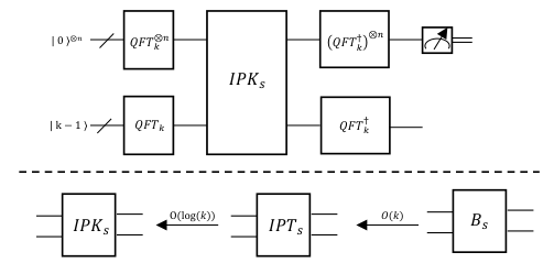
First, we prepare the initial state , where there are registers and each one is associated with a -dimensional Hilbert space.
Second, after quantum Fourier transform , the initial state is changed to
where
with .
At the third step, apply the quantum oracle of
Then, the state evolves to
At the fourth step, after applying inverse quantum Fourier transform , we get the state
Finally, the secret string can be obtained with certainty after measuring the first registers in the computational basis.
Lemma 19.
Let . Then, for
with , we have
Proof.
Let for . Then for some integer , that is,
Then we have
| (30) | ||||
| (31) | ||||
| (32) | ||||
| (33) | ||||
| (34) | ||||
| (35) |
where note that in Eq. (32), holds for integer , and in Eq. (33), when traverses all the values in , so does .
∎
Lemma 20.
Given , can be computed by calling times in parallel.
Proof.
Given and , let . denotes the binary representation of . There is with . Then
where .
∎
Lemma 21.
Given and , can be computed by using black-peg queries in parallel.
Proof.
We now describe how to compute using black-peg queries .
Given , we define strings for as follows:
Feed the black-peg function with , and record the results as
Let
For , obviously there are
| (36) | ||||
| (37) |
Combine Eq. (36) and Eq. (37), we have
Hence, we get
for . That is, we can use the query results to compute for . Now we are ready to compute :
As a result, can be computed by black-peg queries in parallel. ∎